Quantified Advantage of Ghost Imaging over Regular Imaging

Abstract

Ghost imaging has been used in archaeology, bio-medicine, for seeing through turbid media, and promises X-ray imaging improvements, amongst many other applications. However, the advantage of ghost imaging over regular imaging is difficult to quantify. We searched for a simple example that can be quantified with basic statistics. Using classical computational ghost imaging, we find that the signal-to-noise ratio for ghost imaging of a slit (the object) can exceed that of regular imaging with the same exposure of the slit when the detectors are sufficiently noisy. This result is obtained by numerical simulation and by theoretical analysis. We propose an experiment using a spontaneous down-conversion source to demonstrate this quantitative imaging advantage.

I Introduction

Ghost imaging offers the promise to see through “cloudy” objects [1] and to lower the exposure of the object that is to be imaged [2]. The method is technically more involved than regular imaging, and it is hard to find simple demonstrations where ghost imaging is quantitatively shown to be advantageous in comparison to regular imaging in a way that is generally accessible. For example, imaging through turbid media can give contrast better then regular imaging [3], but the Signal-to-Noise Ratio (SNR) was not measured. Exposure claims made for ghost imaging with X-rays [4] have been challenged and are not trivial [5]. A comparison of the SNR of ghost imaging with light sources of a different nature (thermal, low flux, and high flux entangled) has been made [6], but those SNRs were not compared to that of regular imaging. In very specific situations (for example with sparse representation), X-ray and electron ghost imaging using multiplexing offers SNR improvements [7], though the exposure of the object is increased. This can still be advantageous for using more of the incident flux of expensive-to-operate sources, but multiplexing does not offer gain when using photon counting detection. Foundational experiments, like the double-slit experiment, can also benefit from ghost imaging [8]. No quantitative comparisons to regular imaging were made in these examples. Very recently, it was shown that the cost for experiments to do ghost imaging can be lowered [9], and a new single pixel camera for ghost imaging was developed [10]. Both of these experimental efforts are intended for use in an educational setting, but the SNR for these experiments were not provided. Ghost imaging and gated imaging made it possible to obtain high contrast images when using an average of fewer than one detected photon per image pixel [11]. However, a comparison of the SNR with regular imaging was not performed.

We calculated the SNR for 1-D ghost, gated, and regular imaging. The object consists of an aperture with a size of one pixel. The detector noise can be varied. We show that when the detector noise is increased to reduce the SNR of regular imaging to below one, ghost and gated imaging are protected to yield an SNR that is better by an order of magnitude. This result is obtained when the exposure of the object is the same for all three imaging techniques. This result is consistent with that of [11], is easily computed by simulation, and a statistical analysis provides a closed expression which may aid experimental design.

For ghost imaging, photon entangled sources can be used [12]. We apply the analytic expressions for a typical entangled photon source. This may help designs of experiments that could demonstrate quantitatively the ghost imaging advantage over regular imaging.

II Historical Background and Context

Figure 1: Popper’s thought experiment. An entangled particle pair is released from a source, so that their momenta are correlated. Left inset shows slits placed in the path of both particles. Right inset shows the same except slit B is removed. The counter-intuitive consequence is that the spatial resolution improves when slit B is removed. This is explained in the Historical Context section. The narrowing of the peaked coincidence distribution of the particles is a “ghost-like” image of slit A.

Ghost imaging is a method that was used to test Popper’s thought experiment [13]. The Popper’s thought experiment is as shown in figure 1. Such an arrangement was predicted to break the Heisenberg’s uncertainty principle, since the position information from particle 1 going through slit A improves the position information of particle 2, while the momentum information from particle 2 is unchanged. An ever narrower slit A could thus be used to break Heisenberg’s uncertainty principle. After Y.H. Kim et al. performed this bi-photon ghost imaging [13], Heisenberg’s uncertainty principle appears broken for a one particle system. However, using an appropriate description of a two-particle system shows the principle is not broken [14]. The analysis of Popper’s experiment [14] showed that the presence of a lens in [13] prevented testing Popper’s claim and also showed that an earlier experiment ruled out Popper’s idea [15]. Nevertheless, the interesting result remained that the experiment was able to produce images that were of better quality without slit B, since the coincidence peak got narrower as illustrated in figure 1 [16] (p.22). So, it is natural to inspect if there is some regime where ghost imaging surpasses regular imaging.

Shih et al. show ghost imaging for the first time using the spatial correlations produced by parametric down-conversion [15]. The effect was thought to be associated with the entanglement of the photons, but it was shown later that it is possible to perform ghost imaging with classically correlated light beams [17]. Ghost imaging has spurned further progress in quantum imaging, notably the recent work by Zeilinger et al. [18]. Interference between the photons from two down-conversion crystals, pumped with the same source, allows one to retrieve the image even if the beam that interacts with the object is not detected, perhaps more ghostly than ghost imaging.

III Theory

We do a SNR analysis of a regular imaging system and a ghost imaging system to quantify the quality of the image, while making sure that the exposure of the object is the same for both. We start with the derivation of the signal for ghost imaging. Consider the setup in figure 2. A spontaneous down-conversion crystal (SPDC) generates two photons for incident photons. One of these two goes to the camera and the other to the bucket detector. The number of produced photons received by the camera is given by $I_{n}(x_{i})$ at the ”pixel” position $x_{i}$. We call this the $n$-th “realization.” The number of photons in each pixel in the spatial distribution is assumed to be given by a Poisson distribution $X_{i,n}(\lambda)$, where $\lambda=Rt_{w}$ (R is the rate of detected photons per pixel, and $t_{w}$ is the time window). The object is placed in front of the bucket detector. The transmission of the object per pixel at position $x_{i}$ is given by $T(x_{i})$. For each realization $n$, the bucket signal $B_{n}$ is obtained by summing over the pixel position, while an individual ghost image is $I_{n}(x_{i})B_{n}$. Summing over $N$ realizations leads to the final ghost image $G(x_{i})$:

$$I_{n}(x_{i})=X_{i,n}(\lambda)$$ (1)

$$B_{n}=\sum_{i}I_{n}(x_{i})T(x_{i})$$ (2)

$$G(x_{i})=\sum_{n=1}^{N}B_{n}I_{n}(x_{i}).$$ (3)

For regular imaging, we replace the bucket detector with a camera and take the sum of $I_{n}(x_{i})T(x_{i})$ over $N$ realizations:

$$R(x_{i})=\sum_{n=1}^{N}T(x_{i})I_{n}(x_{i}).$$ (4)

In our case, regular imaging is shadow imaging, such as x-ray imaging used in radiology.

Figure 2: Schematic Setup. The correlated source sends spatially correlated photons to the object and the camera’s pixels. After the photons expose the object, the bucket detector collects the transmitted photons, and the correlator multiplies the bucket detector signal with the pixelated image from the camera. This gives us a ghost image for the $n$-th realization. An example ghost image summed over many realizations is shown in the blue bar graph. If we remove the camera and correlator and replace the bucket detector with the camera, we get the setup for regular imaging. If we switch the roles of the bucket detector and camera, we get gated imaging.

III.1 Simulation

The object we consider is a single pixel hole. The image of a single pixel hole consists of one data point in the location $x_{i=m}$ separated from a background of data points in the locations $x_{i\neq m}$. To get the signal, we take the average intensity of the background over the number of background pixels and subtract it from the intensity at point $x_{i=m}$. Thus, the signals of both regular and ghost imaging, denoted by $S_{R}$ and $S_{G}$ respectively, are given by

$$S_{R}=\sum_{n=1}^{N}\left[R(x_{m})-\frac{\sum_{i}R(x_{i\neq m})}{P-1}\right]$$ (5)

$$S_{G}=\sum_{n=1}^{N}\left[G(x_{m})-\frac{\sum_{i}G(x_{i\neq m})}{P-1}\right],$$ (6)

where $P$ is the total number of pixels in the camera.

To get the noise in the signals $S_{R}$ or $S_{G}$, one measurement of the signal is given by Eqs. 5 and 6. The measurement is repeated $K$ times $(k=1,...,K)$ and $\overline{S}$ is the average signal over $K$ measurements. Then, the noise in the signal, given by $\sigma_{S}$, is given by

$$\sigma_{S}=\sqrt{\frac{1}{K}\sum_{k=1}^{K}(S_{k}-\overline{S})^{2}}.$$ (7)

Evaluating Eqs. 1 to 7 will give us the SNR for ghost and regular imaging. By using a Python simulation, we investigate how the SNR for both varies with $\lambda$ in Eq. 1. We are interested in varying $\lambda$ because that determines how much we expose the object $T(x_{i})$. Since we get the image over $N$ realizations, and $\lambda$ is the average exposure of the object per realization, we get the same exposure $N\lambda$ for both regular and ghost imaging.

III.2 Analysis

To verify the simulated result, we derive the SNR for regular and ghost imaging. The single pixel object is described by

$$T(x_{i})=\left\{\begin{array}[]{ll}1,&i=m;\\[5.0pt] 0,&i\neq m.\end{array}\right.$$ (8)

The intensity distribution that is sent to the bucket detector is identical to the one sent to the camera. This distribution is given in terms of photons per pixel by

$$I(x_{i})=X_{i}(\lambda_{s}).$$ (9)

$X_{i}(\lambda_{s})$ is a random Poisson number dependent on $\lambda_{s}$. It is not sufficient to lower $\lambda_{s}$ below one to obtain a ghost imaging advantage over regular imaging (see Results section). After introducing detector dark counts, this situation changes. The dark count in the detectors per pixel is given by

$$J(x_{i})=Y_{i}(\lambda_{d}).$$ (10)

$Y_{i}(\lambda_{d})$ is a random Poisson number dependent on $\lambda_{d}$. The bucket detector signal is

$$\sum_{i}T(x_{i})I(x_{i})+J(x_{i}) =I(x_{m})+J(x_{m})$$

$$=X_{m}(\lambda_{s})+Y_{m}(\lambda_{d}).$$ (11)

The ghost image over $N$ realizations is given by

$$G(x_{i\neq m}) =\sum_{n=1}^{N}(I(x_{m,n})+J(x_{m,n}))(I(x_{i\neq m,n})$$

$$+J(x_{i\neq m,n}))$$

$$=\sum_{n=1}^{N}(X_{m,n}(\lambda_{s})+Y_{m,n}(\lambda_{d}))(X_{i\neq m,n}(\lambda_{s})$$

$$+Y_{i\neq m,n}(\lambda_{d}))$$ (12)

$$G(x_{i=m}) =\sum_{n=1}^{N}(I(x_{m,n})+J(x_{m,n}))^{2}$$

$$=\sum_{n=1}^{N}(X_{m,n}(\lambda_{s})+Y_{m,n}(\lambda_{d}))^{2}.$$ (13)

If the bucket detector were to be replaced by a camera, the regular image is given by

$$R(x_{i\neq m}) =\sum_{n=1}^{N}[T(x_{i\neq m})I(x_{i\neq m,n})+J(x_{i\neq m,n})]$$

$$=\sum_{n=1}^{N}Y_{i\neq m,n}(\lambda_{d})$$ (14)

$$R(x_{i=m}) =\sum_{n=1}^{N}[I(x_{m,n})+J(x_{m,n})]$$

$$=\sum_{n=1}^{N}[X_{m,n}(\lambda_{s})+Y_{m,n}(\lambda_{d})].$$ (15)

By using Eq. 5, the signal of regular imaging measured with $P$ pixels over $N$ realizations is given by

$$S_{R}= \sum_{n=1}^{N}\left[X_{m,n}(\lambda_{s})+Y_{m,n}(\lambda_{d})\right]$$

$$-\sum_{n=1}^{N}\left[\frac{\sum_{i}Y_{i\neq m,n}(\lambda_{d})}{P-1}\right].$$ (16)

By using Eq. 6, the signal of the ghost image measured with $P$ pixels over $N$ realizations is given by

$$S_{G}=\sum_{n=1}^{N}\left[(X_{m,n}(\lambda_{s})+Y_{m,n}(\lambda_{d}))^{2}\right]$$

$$-\sum_{i}\left[\frac{(X_{m,n}(\lambda_{s})+Y_{m,n}(\lambda_{d}))X_{i\neq m,n}(\lambda_{s})}{P-1}\right]$$

$$-\sum_{i}\left[\frac{(X_{m,n}(\lambda_{s})+Y_{m,n}(\lambda_{d}))Y_{i\neq m,n}(\lambda_{d})}{P-1}\right].$$ (17)

Note that the parametrization, in particular $\lambda_{s}$, allows the exposure for regular imaging to be chosen identical to that for ghost imaging. The SNRs of regular imaging and ghost imaging are given by

$$\text{SNR}=\frac{\operatorname*{\mbox{E}}(S)}{\sqrt{\operatorname*{\mbox{Var}}(S)}},$$ (18)

where $\operatorname*{\mbox{E}}(S)$ is the expectation and $\operatorname*{\mbox{Var}}(S)$ is the variance. Using Eq. 16, the SNR of regular imaging is found (see appendix) to be

$$\frac{S_{R}}{\sigma_{S_{R}}}=\frac{\lambda_{s}\sqrt{N}}{\sqrt{\lambda_{s}+\lambda_{d}+\frac{\lambda_{d}}{(P-1)}}}.$$ (19)

Using Eq. 17, the SNR of ghost imaging is found to be

$$\frac{S_{G}}{\sigma_{S_{G}}} =\lambda_{s}\sqrt{N}\bigg{[}\lambda_{s}+3\lambda_{s}^{2}+(\lambda_{s}+\lambda_{d})^{3}$$

$$+(\lambda_{s}+\lambda_{d})^{2}+2\lambda_{d}\lambda_{s}^{2}+2\lambda_{s}\lambda_{d}$$

$$+\frac{(\lambda_{s}+\lambda_{d})^{3}+(\lambda_{s}+\lambda_{d})^{2}}{(P-1)}\bigg{]}^{-1/2}.$$ (20)

where $\lambda_{s}$ is proportional to the source rate, $\lambda_{d}$ is proportional to the detector background rate, $P$ is the number of pixels, and $N$ is the number of realizations.

IV Results

The results of the simulation for ghost and regular imaging are given in figures 3 and 4, along with curves generated from Eqs. 19 and 20. Figure 3 depicts the case where $\lambda_{d}=0$. This indicates that if we had photon detectors with a quantum efficiency of 1, regular imaging is better or equal to ghost imaging. Figure 4 represents the case where the detectors have dark counts characterized by $\lambda_{d}=0.01$. Below $\lambda_{s}=0.1$, the ghost imaging SNR starts to dominate. This can be explained by Eqs. 19 and 20, where the ghost imaging technique suppresses the deleterious effects of the dark count while the regular image drowns in the dark count noise.

Another way to understand this advantage is by comparing ghost imaging to gated imaging. If we switch the roles of the bucket detector and camera in ghost imaging in figure 2, we have a gated imaging setup  [11]. In gated imaging, the camera only looks at the object (within a specified time window) when the bucket detector observes photons from the source. Hence, background noise from the detectors is suppressed in gated imaging, while that is not true for regular imaging. This background suppression also holds for ghost imaging since we are still using the time correlation between the bucket detector and camera. The black data points in figures 3 and 4 represent the SNR for gated imaging as $\lambda_{s}$ is varied. We can observe that the SNR of ghost imaging and gated imaging are identical at low $\lambda_{s}$. The regime where ghost imaging gets a significant advantage over regular imaging is $\lambda_{s}=10^{-4}$, $\lambda_{d}=10^{-2}$, and $N=10^{5}$. The regular and ghost images for these parameters are shown in figures 3 and 4.

Figure 3: Ghost Imaging and Regular Imaging without dark count. The SNR is shown as a function of $\lambda_{s}=R_{s}t_{w}$ ($R_{s}$ is the rate of detected photons per pixel, and $t_{w}$ is the time window). The detector dark count is kept constant at $\lambda_{d}=0$ and the number of realizations $N=10^{5}$. The data points are obtained by the simulation, where blue is ghost imaging and red is regular imaging (black is gated imaging). The solid lines are obtained by the theoretical analysis (Eqs. 19 and 20). Example images are provided at certain points for comparison. In the region where $\lambda_{s}>0.1$, we observe that regular and gated imaging offer better SNR in comparison to ghost imaging. In the region $\lambda_{s}<0.1$, we observe that all three imaging methods produce the same SNR.

Figure 4: Ghost Imaging and Regular Imaging with dark count. The SNR is shown as a function of $\lambda_{s}=R_{s}t_{w}$ ($R_{s}$ is the rate of detected photons per pixel, and $t_{w}$ is the time window). The detector dark count is kept constant at $\lambda_{d}=0.01$ and the number of realizations $N=10^{5}$. The data points are obtained by the simulation, where blue is ghost imaging and red is regular imaging (black is gated imaging). The solid lines are obtained by the theoretical analysis. Example images are provided at certain points for comparison. In the region where $\lambda_{s}>0.1$, we observe that regular and gated imaging offer better SNR in comparison to ghost imaging, as illustrated by the images of the single pixel slit at the point $\lambda_{s}=10$. In the region $\lambda_{s}<0.1$, we observe that ghost imaging and gated imaging produce better images than regular imaging. For $\lambda_{s}=0.0001$, the SNR of ghost imaging is about an order magnitude better than regular imaging, as illustrated by the images at that point.

V Experimental consideration

Given that the SPDC entangled photon source is the workhorse for quantum optics and readily available, we consider the possibility to demonstrate the above discussed ghost imaging advantage with this tool. In SPDC, one $\hbar\omega$ photon generates two $\hbar\omega/2$ photons. The momenta of the $\hbar\omega/2$ photons transverse to the incoming photon direction are equal and opposite, resulting in momentum correlation upon the generation of the photon pair. To obtain the spatial correlation that we need for the approach we analyzed above, one can let the photons freely propagate to detectors placed in the far field.

For a typical SPDC source, one 400 nm photon generates two 800 nm photons. Under typical operation, the avalanche photon detectors record a similar count rate, $R_{s}$, of about $10^{4}$/s 800 nm photons at each detector. The dark count rate of the detectors, $R_{d}$, is about $10^{3}$/s. For a measurement time window $t_{w}$ of the order of 10 ns, the source has $\lambda_{s}=Rt_{w}$ of about $10^{-4}$. In practice, the measurement time cannot be controlled to such a short duration. Instead, one can measure for (for example) a time of $T=1$ ms and consider that to be the equivalent of $N=10^{5}$ realizations of 10 ns measurements for the purpose of obtaining a value for $\lambda_{s}$. The width of each of the two 800 nm beams is about 1 cm on the detector screen (placed 0.5 m away from the SPDC) and are fully separated from each other. For a movable slit of 1 mm width, placed in front of the detector, the detection rate is cut by a factor of $\epsilon=0.1$. The number of counts $N_{s}$ observed per pixel for regular imaging in this example would be $N_{s}=R_{s}\epsilon T=(\lambda_{s}/t_{w})\epsilon(t_{w}N)=1$. The corresponding value of $\lambda_{s}=R_{s}t_{w}=10^{-4}$ is a source strength that is in the regime for which the predicted imaging advantage is clear (see figure 4). The detector dark count strength is $\lambda_{d}=R_{d}t_{w}=10^{-5}$. In this case, a regular image would have an SNR above 1 (similar to the $\lambda_{d}=0$ case), thus the detector noise has to be increased to drown the regular image in the detector noise (as in figure 4, left lower inset).

This can be achieved by increasing the amount of ambient light. This needs to be done in such a way that the ambient light strikes the detector directly and not the object. For $\lambda_{d}=10^{-2}$, the number of counts detected for regular imaging would be $N_{D}=R_{d}T=(\lambda_{d}/t_{w})(t_{w}N)=1000$ (figure 4) with a rate of $R_{d}=10^{6}/s$. In this way one can match the parameters used in the above analysis ($\lambda_{s}=10^{-4}$, $\lambda_{d}=10^{-2}$, $N=10^{5}$). The measured coincident rate $R_{c}$ is about $10^{2}$/s. These coincidences are measured when the two detectors are positioned symmetrically with respect to the axis defined by the incoming photon. The measured coincident rate $R_{c}$ could be as high as $10^{3}$/s$=\epsilon R_{s}$ if both detectors would, without fail, record every photon pair. If one of the detectors is moved laterally by 5 mm, the observed coincidence rate drops to $1$/s, while the singles rate stays nominally the same.

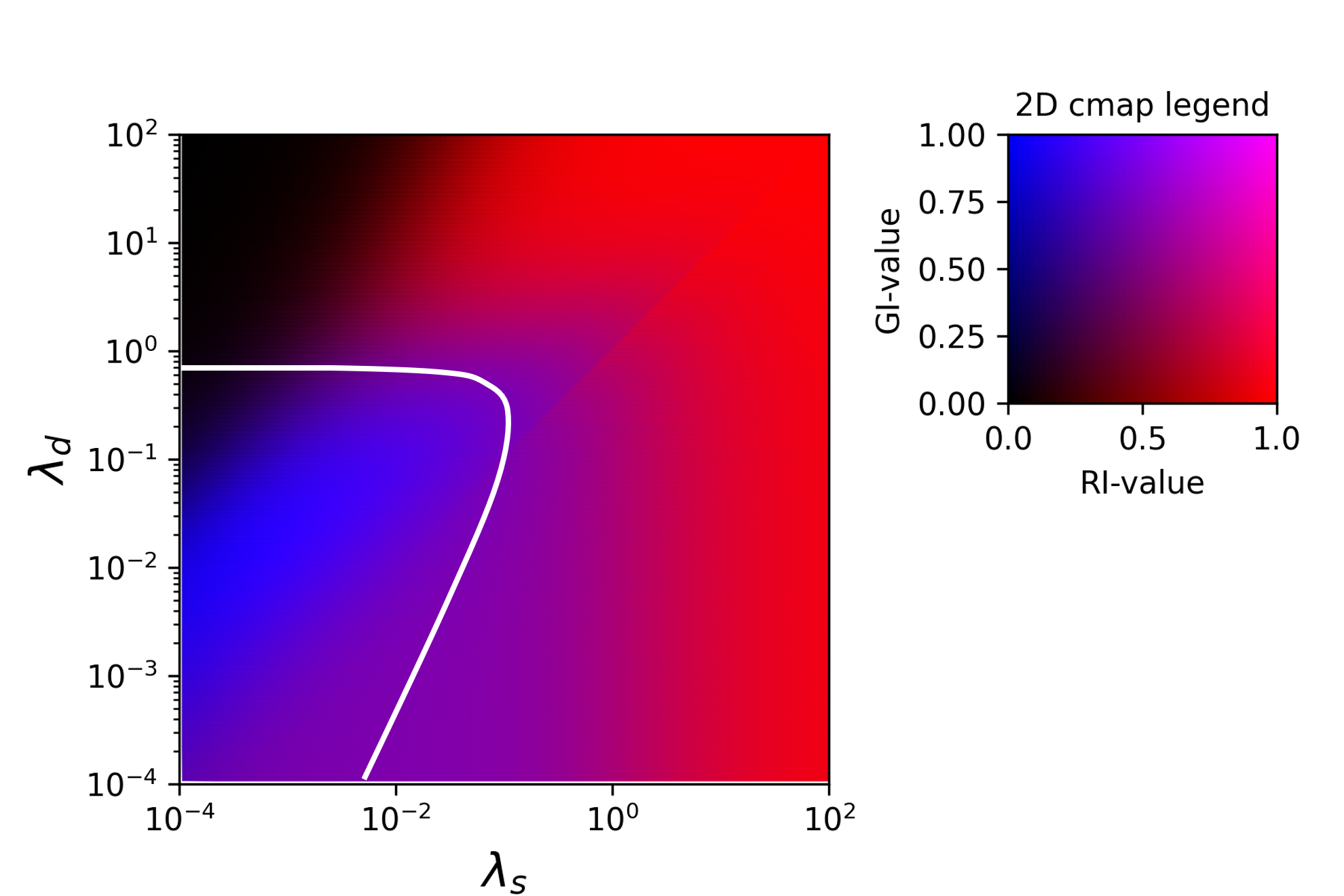
Figure 5: SNR parameter space. For experimental consideration it may be of use to consider the effective SNR as a function $\lambda_{s}$ and $\lambda_{d}$ ($N=10^{5}$). The effective SNR is represented by a color map with a GI-value and RI-value ranging from 0 to 1. The GI/RI-value is defined as $\text{SNR}_{G/R}/(1+\text{SNR}_{R}+\text{SNR}_{G})$. Blue means a dominant ghost imaging SNR, red means a strong regular imaging SNR, purple means both imaging methods contribute to a strong SNR, while black indicates a poor image quality. The white line indicates that the Regular and Ghost Imaging SNR are equal.

.

The measured coincident background rate $N^{(2)}_{bg}$ due to randomly arriving photons (without detection slits) is given by $N^{(2)}_{bg}=R^{2}t_{w}=1/s$. When the detectors noise is raised with ambient light so that again $\lambda_{d}=10^{-2}$, this number increases to $N^{(2)}_{bg}=10^{4}/s$. This means that the SNR for regular imaging and ghost imaging is the same. This rather constructed, but nevertheless representative example indicates that a judicious choice of the slit width, careful alignment of the detectors, temporal and spatial compensation plates [19] could be used to maximize the measured coincidence rate and that an experimental demonstration of this SNR ghost imaging advantage is not trivial, but perhaps within reach.

To design an experiment, it may be of use to vary the parameter $\lambda_{d}$ in addition to $\lambda_{s}$. Figure 5 provides a false color image of the effective SNR of ghost imaging and regular imaging based on Eq. 19 and 20. This indicates for which values in the parameter space each is dominant and where the SNR values exceed one, so that a clear image can be obtained.

VI Summary, Discussion and Conclusion

Our goal was to find a simple computational example where ghost imaging is advantageous over regular imaging. By using the SNR as a metric, we found numerically and analytically a regime that shows that advantage, and we discussed an experiment that could test this regime. We found that ghost imaging suppresses the background detector noise in a similar fashion as compared to gated imaging, while regular imaging does not.

Understanding the advantages of ghost imaging is interesting for many applications. For example, recent ghost imaging developments may find application in bio-medicine and archaeology [20]. Here the advantage is not found in SNR and using low photon rates, but in the use of compressed sensing. Quantum ghost imaging has the additional capability to detect without a bucket detector [21]. These two examples illustrate that our exposition is limited in scope, as ghost imaging advantages depend critically on the specific task, and on the experimental details of the technology used. Nevertheless, considering SNR for low exposures and noisy detectors may be of value in, for example, the context of electron ghost imaging. This recently demonstrated [22] technique has the advantage that the target object could be exposed to fewer electrons. If high-resolution electron ghost imaging can be combined with new methods of protecting biological cells, such as covering the biological specimen with graphene layers [23], this may bring us closer to the dream of seeing living tissue using an electron microscope.

VII Appendix

In statistics, the variance of a quantity $x$ is given by

$$\operatorname*{\mbox{Var}}(x)=\operatorname*{\mbox{E}}(x^{2})-(\operatorname*{\mbox{E}}(x))^{2}.$$ (21)

We need Eq. 21 to solve for $\operatorname*{\mbox{Var}}(S)$ in Eq. 18. Let $x_{1},x_{2},x_{3},...,x_{N}$ be uncorrelated random numbers such that $\operatorname*{\mbox{E}}(x_{i})=\operatorname*{\mbox{E}}(x_{1})$ and $\operatorname*{\mbox{E}}(x_{i}^{2})=\operatorname*{\mbox{E}}(x_{1}^{2})$, where $i\in\{1,2,3,4,...,N\}$. This means $\operatorname*{\mbox{Var}}(x_{i})=\operatorname*{\mbox{Var}}(x_{1})$. Then, by the definition of the expectation value and Bienaymé’s identity [24], we get

$$\operatorname*{\mbox{E}}\left(\sum_{i=1}^{N}x_{i}\right)=N\operatorname*{\mbox{E}}(x_{1})$$ (22)

$$\operatorname*{\mbox{Var}}\left(\sum_{i=1}^{N}x_{i}\right)=\sum_{i=1}^{N}\operatorname*{\mbox{Var}}(x_{i})=N\operatorname*{\mbox{Var}}(x_{1}),$$ (23)

respectively. Given that $S_{G}$ (Eq. 17) depends quadratically on $x$, the variance $\operatorname*{\mbox{Var}}(S)$ defined by Eq. 21 depends quartically on $x$. Therefore, the values of the raw moments for Poisson distributions up to the fourth moment are needed to evaluate Eq. 18. If $x$ is a Poisson random, dependent on $\lambda$, then

$$\operatorname*{\mbox{E}}(x^{k})=\sum_{i=1}^{k}\lambda^{i}S_{t}(k,i)$$ (24)

where $S_{t}$ denotes Stirling numbers of the second kind [25]. Therefore, we get

$$\operatorname*{\mbox{E}}(x)=\lambda$$ (25)

$$\operatorname*{\mbox{E}}(x^{2})=\lambda^{2}+\lambda$$ (26)

$$\operatorname*{\mbox{E}}(x^{3})=\lambda^{3}+3\lambda^{2}+\lambda$$ (27)

$$\operatorname*{\mbox{E}}(x^{4})=\lambda^{4}+6\lambda^{3}+7\lambda^{2}+\lambda.$$ (28)

References

- Yuan and Chen [2022] Y. Yuan and H. Chen, Unsighted ghost imaging for objects completely hidden inside turbid media, New Journal of Physics 24, 043034 (2022).
- Batelaan [2022] H. Batelaan, Shining light on electron microscopy, Physics 15, 145 (2022).
- Bina et al. [2013] M. Bina, D. Magatti, M. Molteni, A. Gatti, L. A. Lugiato, and F. Ferri, Backscattering differential ghost imaging in turbid media, Phys. Rev. Lett. 110, 083901 (2013).
- Zhang et al. [2018] A.-X. Zhang, Y.-H. He, L.-A. Wu, L.-M. Chen, and B.-B. Wang, Tabletop x-ray ghost imaging with ultra-low radiation, Optica 5, 374 (2018).
- Kingston et al. [2021] A. M. Kingston, W. K. Fullagar, G. R. Myers, D. Adams, D. Pelliccia, and D. M. Paganin, Inherent dose-reduction potential of classical ghost imaging, Phys. Rev. A 103, 033503 (2021).
- Erkmen and Shapiro [2009] B. I. Erkmen and J. H. Shapiro, Signal-to-noise ratio of gaussian-state ghost imaging, Phys. Rev. A 79, 023833 (2009).
- Lane and Ratner [2020] T. J. Lane and D. Ratner, What are the advantages of ghost imaging? multiplexing for x-ray and electron imaging, Optics Express 28, 5898 (2020).
- Aspden et al. [2016] R. S. Aspden, M. J. Padgett, and G. C. Spalding, Video recording true single-photon double-slit interference, American Journal of Physics 84, 671 (2016).
- Aguilar et al. [2019] R. A. Aguilar, N. Hermosa, and M. N. Soriano, Low-cost fourier ghost imaging using a light-dependent resistor, American Journal of Physics 87, 976 (2019).
- Kuusela [2019] T. A. Kuusela, Single-pixel camera, American Journal of Physics 87, 846 (2019).
- Morris et al. [2015] P. A. Morris, R. S. Aspden, J. E. Bell, R. W. Boyd, and M. J. Padgett, Imaging with a small number of photons, Nature communications 6, 1 (2015).
- Lin et al. [2021] Z. Lin, L. Schweickert, S. Gyger, K. D. Jöns, and V. Zwiller, Efficient and versatile toolbox for analysis of time-tagged measurements, Journal of Instrumentation 16 (08), T08016.
- Kim and Shih [1999] Y.-H. Kim and Y. Shih, Experimental realization of popper’s experiment: Violation of the uncertainty principle?, Foundations of Physics 29, 1849 (1999).
- Qureshi [2012a] T. Qureshi, Analysis of popper’s experiment and its realization, Progress of Theoretical Physics 127, 645 (2012a).
- Pittman et al. [1995] T. B. Pittman, Y. Shih, D. Strekalov, and A. V. Sergienko, Optical imaging by means of two-photon quantum entanglement, Physical Review A 52, R3429 (1995).
- Qureshi [2012b] T. Qureshi, Popper’s experiment: A modern perspective, arXiv preprint arXiv:1206.1432 (2012b).
- Bennink et al. [2002] R. S. Bennink, S. J. Bentley, and R. W. Boyd, “two-photon” coincidence imaging with a classical source, Physical review letters 89, 113601 (2002).
- Lemos et al. [2014] G. B. Lemos, V. Borish, G. D. Cole, S. Ramelow, R. Lapkiewicz, and A. Zeilinger, Quantum imaging with undetected photons, Nature 512, 409 (2014).
- Altepeter et al. [2005] J. B. Altepeter, E. R. Jeffrey, and P. G. Kwiat, Phase-compensated ultra-bright source of entangled photons, Optics Express 13, 8951 (2005).
- Klein et al. [2022] Y. Klein, O. Sefi, H. Schwartz, and S. Shwartz, Chemical element mapping by x-ray computational ghost fluorescence, Optica 9, 63 (2022).
- Gilaberte Basset et al. [2019] M. Gilaberte Basset, F. Setzpfandt, F. Steinlechner, E. Beckert, T. Pertsch, and M. Gräfe, Perspectives for applications of quantum imaging, Laser & Photonics Reviews 13, 1900097 (2019).
- Li et al. [2018] S. Li, F. Cropp, K. Kabra, T. Lane, G. Wetzstein, P. Musumeci, and D. Ratner, Electron ghost imaging, Physical review letters 121, 114801 (2018).
- Koo et al. [2020] K. Koo, K. S. Dae, Y. K. Hahn, and J. M. Yuk, Live cell electron microscopy using graphene veils, Nano letters 20, 4708 (2020).
- Loeve [1977] M. Loeve, Elementary probability theory, in Probability theory i (Springer, 1977) pp. 1–52.
- Riordan [1937] J. Riordan, Moment recurrence relations for binomial, poisson and hypergeometric frequency distributions, The Annals of Mathematical Statistics 8, 103 (1937).