Asymptotics for the Number of Random Walks
in the Euclidean Lattice

Abstract

We give precise asymptotics to the number of random walks in the standard orthogonal lattice in $\mathbb{R}^{d}$ that return to the starting point at step $2n$, both for all such walks and for the ones that return for the first time. The first set of asymptotics is obtained in an elementary way, by using a combinatorial and geometric multiplication principle together with the classical theory of Legendre polynomials. As an easy consequence we obtain a unified proof of Pólya’s theorem. By showing that the relevant generating functions are $\Delta$-analytic, we use the deeper Tauberian theory of singularity analysis to obtain the asymptotics for the first return paths.

2020 Mathematics Subject Classification: Primary 05A16; Secondary 05A10, 40E99, 33C45.

Keywords: random walk, multiplication principle, return probability, asymptotics, Legendre polynomials, $\Delta$-analyticity, Tauberian theory, singularity analysis, Pólya’s theorem.

1 Introduction

Random walks have been studied extensively for more than a century in connection to Brownian motion, diffusion, behaviour of financial time series, and that of many other stochastic processes. In this paper, we think of random walks as occurring in an Euclidean space $\mathbb{R}^{d}$, along the directions of a fixed orthogonal system of coordinates, with equally likely probability of motion in the direction of the axes. We present some interesting connections that random walks afford between combinatorics, geometry, the theory of Legendre polynomials, and the modern Tauberian theory of singularity analysis.

The first part of our paper has combinatorial and geometric themes and presents two multiplication principles satisfied by the number of walks ending at various points in $\mathbb{R}^{d}$. Let $A_{2n}^{(d)}$ denote the number of walks of length $2n$ in $\mathbb{R}^{d}$ that return at the origin at time $t=2n$. Similarly, we denote by $B_{2n}^{(d)}$ the number of walks of length $2n$ in $\mathbb{R}^{d}$ that return for the first time at the origin at time $t=2n$. As part of our results in Section 2, we obtain (see Corollary 2) the following recurrence relation:

$$A_{2n}^{(d+1)}=\binom{2n}{n}\cdot\sum_{k=0}^{n}\binom{n}{k}^{2}\,\frac{A_{2k}^{(d)}}{\binom{2k}{k}}.$$

The main results of the paper are contained in Section 3. In Subsection 3.2 we obtain the asymptotics

$$A_{2n}^{(d)}=\frac{d^{d/2}}{2^{d-1}}\frac{(2d)^{2n}}{(\pi n)^{d/2}}\left(1+O_{d}(1/n)\right)$$

and show how we can continue the development up to any fixed power $k$ of $1/n$, with error $O_{d,k}(1/n^{k+1})$.

These results are proved in a relatively elementary way using the theory of Legendre polynomials and standard results about integrals and Taylor series of basic functions like $\exp$ and $\log$, while using from Section 2 only the above recurrence and the initial conditions for $d=1$. More precisely, denoting by $x_{n}^{(d)}=\frac{A_{2n}^{(d)}}{{2n\choose n}}$, we use the corresponding recurrence

$$x_{n}^{(d+1)}=\sum_{k=0}^{n}\binom{n}{k}^{2}x_{k}^{(d)},\text{ with }x_{n}^{(1)}=1.$$

The core of the argument lies in the fact that, if $\displaystyle{P_{n}(x)=\tfrac{1}{2^{n}n!}\tfrac{d^{n}}{dx^{n}}(x^{2}-1)^{n}}$ are the Legendre polynomials of degree $n$, Leibniz’s rule leads to the recurrence:

$$P_{n}(x)=\left(\frac{x-1}{2}\right)^{n}\sum_{k=0}^{n}{n\choose k}^{2}\left(\frac{x+1}{x-1}\right)^{k}.$$

This immediately suggests that we can use the recurrence for $x_{n}^{(d)}$ and the asymptotics of the Legendre polynomial, in the form

$$(y-1)^{n}P_{n}(x)=\frac{1}{\sqrt{\pi n}}\frac{(\sqrt{y}+1)^{(2n+1)}}{2y^{1/4}}(1+O(1/n)),\text{ with }y=\tfrac{x+1}{x-1},$$

to obtain inductively asymptotics for $x_{n}^{(d)}$ and hence for $A_{2n}^{(d)}$, as long as we can handle the successive powers of $n^{1/2}$ introduced at each step when we raise the dimension by one. This is achieved by the standard elimination method in asymptotic theory, which replaces these powers by simple integrals.

In Subsection 3.3 we use the deeper Tauberian theory of singularity analysis [Flajolet] to obtain asymptotics for the first return paths in the form

$$B_{2n}^{(d)}=\frac{d^{d/2}}{m_{d}^{2}\cdot 2^{d-1}}\frac{(2d)^{2n}}{(\pi n)^{d/2}}(1+O_{d}(1/n)),\text{ for }d\geq 3\text{ and }d\neq 4,$$

while

$$B_{2n}^{(4)}=\frac{2}{m_{4}^{2}}\frac{8^{2n}}{(\pi n)^{2}}(1+O(\log n/n)).$$

Here, for all $d\geq 3$, $m_{d}$ is the expected number of returns to the origin, plus one:

$$1<m_{d}=1+\sum_{n=1}^{\infty}\frac{A_{2n}^{(d)}}{(2d)^{2n}}<\infty.$$

We also obtain asymptotic expansions for the (normalized) generating functions of the sequences $(A_{2n}^{(d)})_{n}$ and $(B_{2n}^{(d)})_{n}$ in terms of the standard functions $T(w)=1-w$ and $L(w)=-\log(1-w)$, $|w|<1$.

While this subsection follows to a large extent the methods expounded in [Flajolet] and especially their zigzag algorithm, in order to apply those we need to prove that our generating functions of $A$ and $B$ satisfy the technical condition of $\Delta$-analyticity. This condition essentially means that the generating functions are analytically continuable at all points on their circle of convergence $|w|=\frac{1}{(2d)^{2}}$, except at the singular positive value $w=\frac{1}{(2d)^{2}}$, and that the continuation works on a domain that is suitable to contain keyhole contours around the singularity. For details and geometric conditions for such a domain see Subsection 3.3. In order to prove $\Delta$-analyticity, we again use properties of the Legendre polynomials, this time in the complex domain, and especially the identity

$$\sum_{m=0}^{\infty}{n+m\choose m}^{2}w^{m}=(1-w)^{-n-1}P_{n}\left(\frac{1+w}{1-w}\right),\text{ for }|w|<1,$$

which seems to have a long history, appearing as early as 1303 (in the form of the equality between the coefficients of $w^{k}$ on both sides) in the works of the Chinese mathematician Shih-Chieh Chu ([Takacs]).

In Section 4, we conclude the paper with a unified proof of Pólya’s theorem based on the results from Subsections 3.1 and 3.2.

The first multiplication principle, as stated in this paper, was obtained in a research for undergraduates project conducted at Adrian College by the first author with Jamie Brandon. That project was about random walks in 2D Euclidean domains with boundary and we hope to present some of those findings somewhere else.

2 Simple random walks in Euclidean spaces

To set up the discussion, consider the Euclidean space $\mathbb{R}^{d}$, with a fixed system of coordinates. We will use the lattice with vertices the points with integer coefficients and with each vertex being joined to the nearest neighbors by an undirected segment. By a (simple) random walk of length $n$ we understand the motion of a point which starts at the origin $P_{0}$ and “walks” along $n$ segments of the lattice, at each vertex choosing with equal probability $1/(2d)$ which segment to follow next. Sometimes we refer to the number of traveled segments as time, because this set-up corresponds to a discrete-time and discrete-space walk, one step of the walk occurring with each increment of the time $t$. In this section we obtain explicit formulas for the number of random walks of length $n$ that end up at a particular point in $\mathbb{R}^{d}$, when the starting point is fixed. In other words, we determine the geometric distribution of these numbers. See Figure 1 below.

2.1 Random walks in $\mathbb{R}^{2}$ and the first multiplication principle

We begin by analyzing walks in the plane which start, for simplicity, at the origin of the coordinate system. In the first step, $n=1$, the starting point $P_{0}=(0,0)$ contributes four possible paths: one that moves up, left, right, and down, respectively. Similarly, in the second step, $n=2$, the end of each path of length 1 contributes four more paths. The figure below shows this distribution in the case $n=3$ and $n=4$. Each green dot represents the end of a path. The number next to a dot represents the number of paths that end at that green dot, among all possible walks of length $n$. The gray dots are the ends of paths from the previous time step.

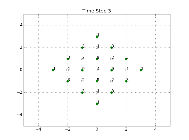
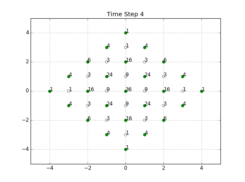
Figure 1: The diamond shaped distribution of random walks starring at $P_{0}=(0,0)$.

This gives a fairly clear inductive procedure: to find the number of paths of length $n$ that end at a given point, we look at the previous time step and sum the number of paths of length $n-1$ from the places above, left, right, and below of the given point. It follows immediately from this that the numbers appearing on the sides of the diamond are the binomial coefficients of $n$. The inner values also follow a pattern, that we refer to as the first multiplication principle:

Lemma 1.

The number of random walks of length $n$ in the plane that start at the origin $(0,0)$ and end at point $(k,l)$ is given by $\displaystyle{\binom{n}{\frac{n+k-l}{2}}\binom{n}{\frac{n+k+l}{2}}}.$ Here, $-n\leq k\leq n$, $-n\leq l\leq n$, $|k|+|l|\leq n$, and $n\equiv k+l\pmod{2}$.

Remark 1.

In its essence, Lemma 1 is due to the fact that a random walk in $\mathbb{R}^{2}$ can be viewed as the product of two independent one-dimensional random walks. This is clear if one projects the walk on the orthogonal system consisting of the diagonals of the standard system of coordinates. It is mentioned in [FFK, Example 12], [Flajolet, Example VI.14], and, in the disguised form of generating functions, in [Finch, page 323]. Perhaps the proof below, which is purely combinatorial, will make it better known and appreciated.

Remark 2.

The formula in Lemma 1 looks complicated because it references correctly the cartesian coordinates $(k,l)$ of the end point, but the idea is very simple. We call this a multiplication principle because it can be viewed as a multiplication table of a sort. Let $C_{n}$ denote the $1\times(n+1)$ row matrix with entries the binomial coefficients of $n$: $C_{n}=\left[\begin{array}[]{cccccc}\binom{n}{0}&\binom{n}{1}&\cdots&\binom{n}{i}&\cdots&\binom{n}{n}\end{array}\right].$ The number of random walks of length $n$ is encoded in the matrix $W_{n}=C_{n}^{T}\cdot C_{n}=(w_{ij})_{1\leq i,j\leq n+1}$, with $w_{ij}=\binom{n}{i-1}\binom{n}{j-1}$. In order to obtain the diamond of numbers shown in Figure 1, this matrix has to be rotated by 45°, then scaled and shifted such that its entries overlap correctly with the position of end points of the random walks.

Proof.

We use induction on $n$. The case $n=1$ is obvious. Assume that the result holds for $n$. At step $n+1$, the boundary of the diamond is clearly given by the binomial coefficients, while for $2\leq i,j\leq n+1$ the number on row $i$ and column $j$ is obtained by adding the adjacent numbers at step $n$, as indicated in the diagram below.

$$\begin{array}[]{rrcll}&&\binom{n}{i-2}\binom{n}{j-2}&&\\ &&\downarrow&&\\ \binom{n}{i-1}\binom{n}{j-2}&\to&?&\leftarrow&\binom{n}{i-2}\binom{n}{j-1}\\ &&\uparrow&&\\ &&\binom{n}{i-1}\binom{n}{j-1}&&\\ \end{array}$$

The four shown numbers add up to $\binom{n+1}{i-1}\binom{n+1}{j-1}$ and this finishes the proof. ∎

2.2 Random walks in $\mathbb{R}^{3}$

The three-dimensional case is slightly more complicated. There is no equivalent of Lemma 1, perhaps not surprisingly because the $l^{1}$ unit ball is not a cube, but a different multiplication principle holds. The end points of all possible random walks of a fixed length form octahedra and a multiplication principle which holds on the faces of such octahedra turns out to hold for “layers” too (see below). Moreover, the result that we were able to first observe for $\mathbb{R}^{3}$ turns out to hold for any $\mathbb{R}^{d}$, with $d\geq 3$. See Theorem 2.

We need to introduce some notation. For $n\geq 0$ and with the convention that $\binom{0}{0}=1$, recall that we denoted with $C_{n}$ the $1\times(n+1)$ row matrix with entries the binomial coefficients of $n$. Let $T_{n}$ denote the Pascal’s triangle containing the binomial coefficients up to and including $n$. We build inductively a new sequence of triangles of numbers $(\mathbf{\tau_{n}})_{n\geq 0}$ using the following procedure. At stage $n=0$, $\mathbf{\tau_{0}}$ consists just of number 1. At any subsequent stage $n+1$, the numbers from $\mathbf{\tau_{n}}$ duplicate one slot above, to the left, and to the right, and then they are removed from the triangle. The new triangle $\mathbf{\tau_{n+1}}$ consists of the sums of the numbers that so result at each location. The diagram bellow shows the first five triangles of this sequence.

$$\begin{array}[]{c}\\ \\ \\ \\ 1\\ \mathbf{\tau_{0}}\end{array}\qquad\begin{array}[]{rcl}&&\\ &&\\ &&\\ &1&\\ 1\!\!&&\!\!1\\ &\mathbf{\tau_{1}}&\end{array}\qquad\begin{array}[]{rrcll}&&&&\\ &&&&\\ &&1&&\\ &2\!\!&&\!\!2&\\ 1\!\!&&2&&\!\!1\\ &&\mathbf{\tau_{2}}&&\end{array}\qquad\begin{array}[]{ccccccc}&&&&&&\\ &&&1&&&\\ &&3\!\!&&\!\!3&&\\ &3\!\!&&6&&\!\!3&\\ 1\!\!&&3\!\!&&\!\!3&&\!\!1\\ &&&\mathbf{\tau_{3}}&&&\end{array}\qquad\begin{array}[]{ccccccccc}&&&&1&&&&\\ &&&4\!\!&&\!\!4&&&\\ &&6\!\!&&12&&\!\!6&&\\ &4\!\!&&12\!\!&&\!\!12&&\!\!4&\\ 1\!\!&&4\!\!&&6&&\!\!4&&\!\!1\\ &&&&\mathbf{\tau_{4}}&&&&\end{array}$$

We can now state our second multiplication principle:

Lemma 2.

Counting the rows from the top and the location on rows from left to right, the $j$-th number on the $i$-th row in $\mathbf{\tau_{n}}$ equals $\binom{n}{i-1}\cdot\binom{i-1}{j-1}$. In other words, $\mathbf{\tau_{n}}=C_{n}^{T}\times T_{n}$.

Remark 3.

As in Remark 2, we call this a multiplication principle not because the answer is given by the product of two binomial coefficients but because it can be viewed as a multiplication table of a sort, with rows indexed by the binomial coefficients, represented by $C_{n}^{T}$, and the other “dimension” represented this time by the Pascal triangle $T_{n}$. Here is a graphical representation of this description of $\mathbf{\tau_{n}}$:

$$\begin{array}[]{ccccccccccccccc}\binom{n}{0}&&&&&&&&\!\!\!\binom{n}{0}\mathbf{\binom{0}{0}}&&&&&&\\ &&&&&&&&&&&&&&\\ \binom{n}{1}&&&&&&&\!\!\!\binom{n}{1}\mathbf{\binom{1}{0}}&&\!\!\!\binom{n}{1}\mathbf{\binom{1}{1}}&&&&&\\ &&&&&&&&&&&&&&\\ \binom{n}{2}&\mathbf{\times T_{n}=}&&&&&\binom{n}{2}\mathbf{\binom{2}{0}}&\!\!\!&\!\!\!\binom{n}{2}\mathbf{\binom{2}{1}}&&\!\!\!\binom{n}{2}\mathbf{\binom{2}{2}}&&&&\\ \vdots&&&&&\!\!\!\iddots&&&\!\!\!\vdots&&&\!\!\!\ddots&&&\\ \binom{n}{i}&&&&\!\!\!\binom{n}{i}\mathbf{\binom{i}{0}}&\!\!\!\cdots&&&\!\!\!\cdots&\!\!\!\binom{n}{i}\mathbf{\binom{i}{j}}&\!\!\!\cdots&&\!\!\!\binom{n}{i}\mathbf{\binom{i}{i}}&&\\ \vdots&&&\!\!\!\iddots&&&&&\!\!\!\vdots&&&&&\!\!\!\ddots&\\ \binom{n}{n}&&\binom{n}{n}\mathbf{\binom{n}{0}}&\!\!\!&\!\!\!\binom{n}{n}\mathbf{\binom{n}{1}}&\!\!\!\cdots&&&\!\!\!\cdots&\!\!\!\binom{n}{n}\mathbf{\binom{n}{j}}&\!\!\!\cdots&&&&\!\!\!\binom{n}{n}\mathbf{\binom{n}{n}}\end{array}$$

Proof.

We use induction on $n$. The case $n=1$ is clear. Assume that the result holds for $n$. At step $n+1$, on the edges we have the binomial coefficients, from the very way these may be constructed inductively. Consider the $j$-th number on the $i$-th row in $\mathbf{\tau_{n+1}}$, with $0<j<i$. It is obtained by summing the numbers from $\mathbf{\tau_{n}}$ located at position $j-1$ and $j$ on row $i-1$, and that on position $j$ on row $i$. Using the induction hypothesis, this reads:

$$\begin{array}[]{rrcll}\binom{n}{i-2}\binom{i-2}{j-2}&\to&?&\leftarrow&\binom{n}{i-2}\binom{i-2}{j-1}\\ &&\uparrow&&\\ &&\binom{n}{i-1}\binom{i-1}{j-1}&&\\ \end{array}$$

The result now follows from simple algebra. ∎

The triangle $\mathbf{\tau_{n}}$ gives the count of the number of random walks of length $n$ in $\mathbb{R}^{3}$ which start at the origin and end on the faces of the octahedron (the $l^{1}$-sphere of radius $n$ in $\mathbb{R}^{3}$). In terms of walks, the above second multiplication principle can be restated as follows: the number of random walks of length $n$ in the 3D-space which start at $(0,0,0)$ and end at point $(k,l,m)$, where $k,l,m\geq 0$ and $k+l+m=n$, is given by $\binom{n}{m}\cdot\binom{k+l}{l}=\binom{n}{k+l}\cdot\binom{k+l}{l}.$ Perhaps surprisingly, it turns out that these numbers are exactly the ones that describe how all the paths distribute in the 3D-case, as long as we focus on how the distribution of paths happens in entire planes $z=h$, instead of at individual points. A few more definitions and notations are needed in order to justify this observation.

For any integers $n\geq 1$ and $-n\leq h\leq n$, we call the layer at height $h$ of walks of length $n$, denoted $L_{n,h}$, the distribution of number of simple random walks of length $n$ that end in the plane $z=h$. These layers provide a decomposition in horizontal “slices” of the octahedron of paths as depicted in Figure 2.

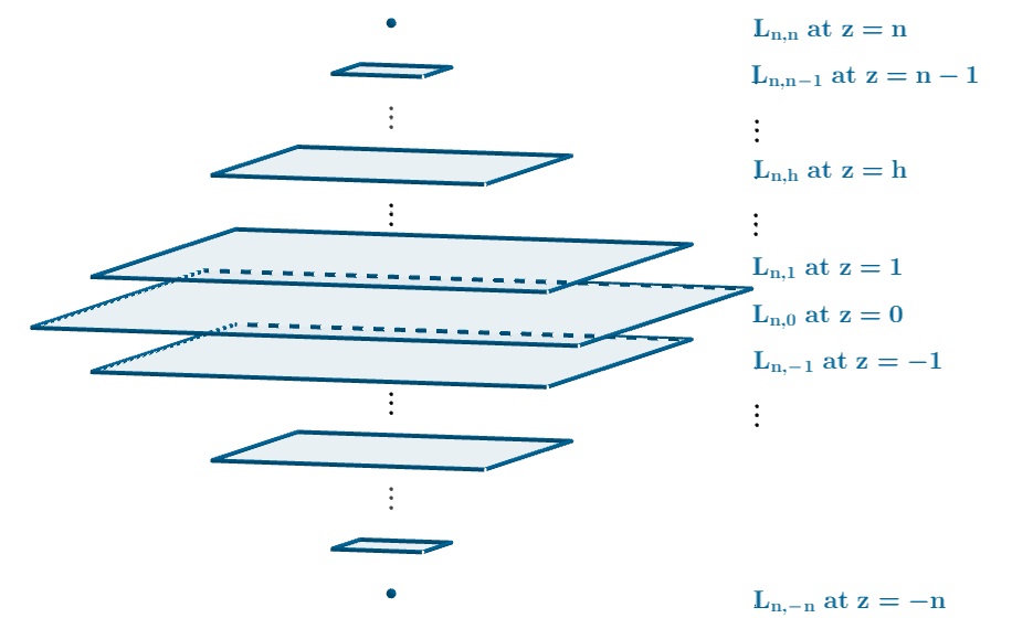
Figure 2: Slicing the octahedron of possible end points with the “layers” $L_{n,h}$.

These layers can also be expressed in an exact form using the 2D-distribution of paths of length $n$, which we denote by $l_{n}$, provided by Lemma 1. (See also Figure 1.) Imagine that the rows of the triangle $\mathbf{\tau_{n}}$ are formally multiplied with $l_{n}$, $l_{n-1}$, …, $l_{1}$, and $l_{0}$, respectively. Then, in this multiplied $\mathbf{\tau_{n}}$, the formal addition of the entries on each column gives the layers $L_{n,h}$, for $-n\leq h\leq n$. The addition is performed by keeping the 2D-distributions centered at the origin. Figure 3 provides a visualization of this in the case when $n=3$ and $n=4$.

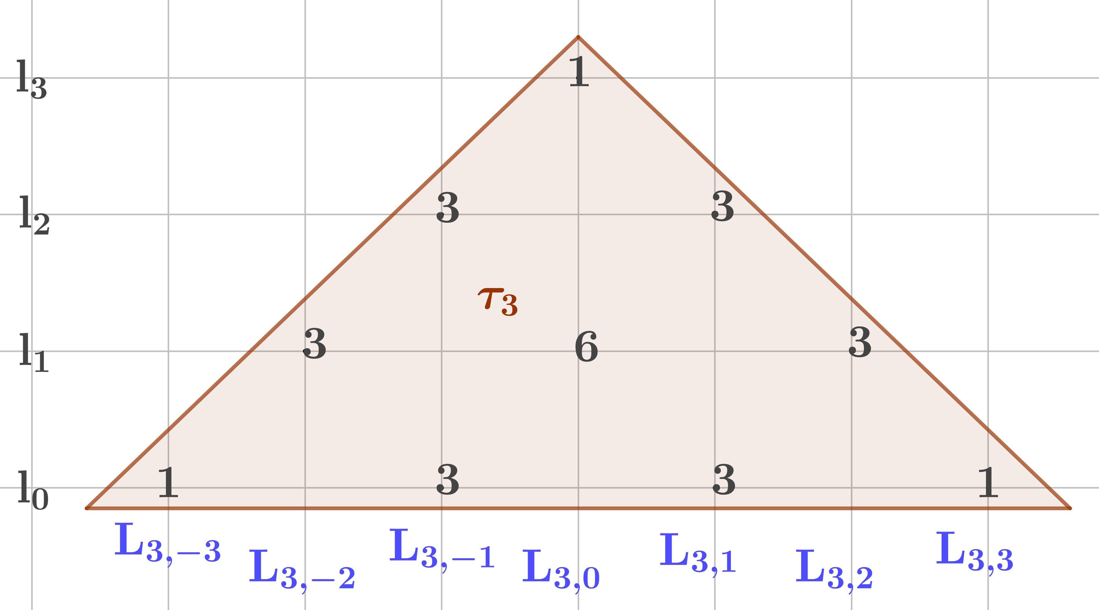
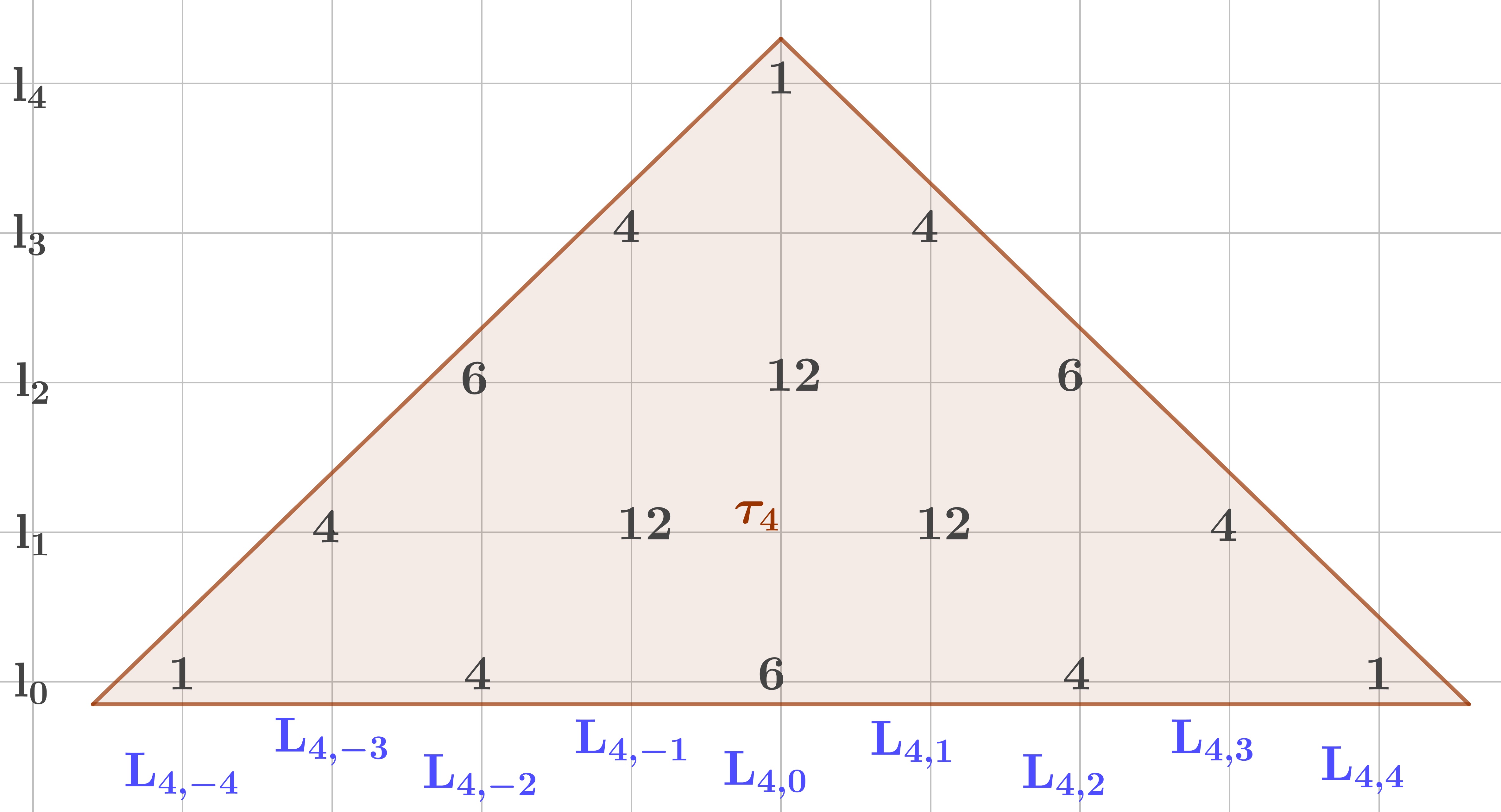
Figure 3: Obtaining the $L_{n,h}$’s as linear combinations of the 2D-distributions, with coefficients from $\mathbf{\tau_{n}}$, in the case when when $n=3$ and $n=4$.

It is easy to see that $L_{n,n}=l_{0}$ and $L_{n,n-1}=n\cdot l_{1}$. We formalize these observations in the following theorem, which shows how to obtain the geometric distribution of walks in dimension $d+1$ from the geometric distribution in dimension $d$, using the second multiplication principle.

Theorem 1.

With the above notations, for all $n\geq 1$ and $0\leq h\leq n$,

$$L_{n,h}=\sum_{j=0}^{\lfloor\frac{n-h}{2}\rfloor}\binom{n}{n-h-2j}\binom{h+2j}{j}l_{n-h-2j}=\sum_{i=0\text{ or }1}^{n-h}\binom{n}{i}\binom{n-i}{\frac{n-h-i}{2}}l_{i}.$$ (1)

In the second sum, $i\equiv n-h\pmod{2}$.

Proof.

Proof by induction on $n$. The case $n=1$ is clear: $L_{1,0}=l_{1}=\binom{1}{1}\binom{0}{0}l_{1}$ and $L_{1,1}=l_{0}=\binom{1}{0}\binom{1}{0}l_{0}$.

The key observation is that the random walks of length $n+1$ are obtained from the layers of the walks of length $n$, where each layer $L_{n,h}$ does only two “moves:” either is expands horizontally in the plane $z=h$, as if the walks were two-dimensional, or it duplicates above and below, in the planes $z=h+1$ and $z=h-1$, respectively.

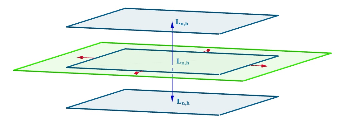
Figure 4: Expansion and duplication of layers, as the length of paths increases.

If one interprets the $j$th column of $\mathbf{\tau_{n}}$ as keeping track of what is going on in the plane $z=j-(n+1)$, then the observation that we just have made about the propagation of layers has the following interpretations. The horizontal expansion of a layer can be tracked by an upward addition ($l_{k}$ becomes $l_{k+1}$). The vertical duplications translate into left and right duplications (the horizontal planes are changed). But this is exactly how $\mathbf{\tau_{n+1}}$ is generated from $\mathbf{\tau_{n}}$. In other words, the sequence $(\mathbf{\tau_{n}})_{n}$ keeps track of the propagation of random walks!

Figure 5: Understanding the change in layers via $\mathbf{\tau_{n}}$.

Finally, the formula given in the statement of the theorem simply uses the numbers from $\mathbf{\tau_{n}}$ to compose $L_{n,h}$ out of the corresponding 2d-distributions $l_{i}$. ∎

Denote with $A_{2m}^{(3)}$ the number of walks of length $2m$ that return at the origin at time $t=2m$. By letting $n=2m$ and $h=0$ in Equation (1), several ways of expressing the number of returning paths can be deduced:

Corollary 1.

 

1. $$A_{2m}^{(3)}=\sum_{j=0}^{m}\binom{2m}{2m-2j}\binom{2j}{j}\binom{2m-2j}{m-j}^{2}=\sum_{k=0}^{m}\binom{2m}{2k}\binom{2m-2k}{m-k}\binom{2k}{k}^{2}.$$ (2)

2. $$A_{2m}^{(3)}=\binom{2m}{m}\cdot\sum_{k=0}^{m}\binom{m}{k}^{2}\frac{A_{2k}^{(2)}}{\binom{2k}{k}}.$$ (3)

3. $$A_{2m}^{(3)}=\sum_{k=0}^{m}\frac{(2m)!\cdot(2k)!}{[(m-k)!]^{2}\cdot[k!]^{4}}.$$ (4)

Remark 4.

From Part (i) one can obtain the formula from [Finch, page 323], namely $A_{2m}^{(3)}=\binom{2m}{m}\cdot\sum_{k=0}^{m}\binom{m}{k}^{2}\binom{2k}{k}.$ This formula and the value of returning walks from dimension two, proves Part (ii) which gives the key recurrence relation which allows us to generate the $A_{2m}^{(3)}$ from the $A$’s in dimension 2. This recurrence relation can be generalized in any dimension; see Corollary 2 further below. Part (iii) indicates that the triple convolution of a particular function might somehow be involved in generating these numbers.

2.3 Walks in any $\mathbb{R}^{d}$

In the previous subsection, we carefully explained the 3D-case for two reasons. First, in view of Pólya’s theorem, this is the most important of the higher dimensions, while still possible to visualize. Second, we believe that the more involved notation that follows would have obscured the simplicity of our proofs. We show next that what we proved for $\mathbb{R}^{3}$ holds true for any $\mathbb{R}^{d}$, with $d\geq 2$, which provides an inductive way of completely understanding the distribution of walks in any Euclidean space.

For any $d\geq 1$, denote by $l_{n}^{(d)}$ the distribution of all random walks of length $n$ in $\mathbb{R}^{d}$. We have: $l_{n}^{(1)}$ is given by $C_{n}$, the binomial coefficients, $l_{n}^{(2)}$ is a diamond, as described by Lemma 1, and $l_{n}^{(3)}$ is an octahedron, as discussed in the previous subsection. Denote by $L_{n,h}^{(d+1)}$ the “layer” of the distribution of random walks of length $n$ in $\mathbb{R}^{d+1}$ contained in the hyperplane $x_{d+1}=h$.

Theorem 2.

With the above notations, for all $d\geq 1$, $n\geq 1$, and $0\leq h\leq n$,

$$L_{n,h}^{(d+1)}=\sum_{i=0\text{ or }1}^{n-h}\binom{n}{i}\binom{n-i}{\frac{n-h-i}{2}}l_{i}^{(d)},$$ (5)

where $i\equiv n-h\pmod{2}$.

Proof.

Identical to the proof of Theorem 1. ∎

Extending the notation before Corollary 1, for any $d\geq 1$, we denote by $A_{2m}^{(d)}$ the number of walks of length $2m$ in $\mathbb{R}^{d}$ that return at the origin at time $t=2m$, for all $m\geq 0$ and with the convention $A_{0}^{(d)}=1$.

Corollary 2.

For any $d\geq 1$,

$$A_{2m}^{(d+1)}=\binom{2m}{m}\cdot\sum_{k=0}^{m}\binom{m}{k}^{2}\,\frac{A_{2k}^{(d)}}{\binom{2k}{k}}.$$ (6)

Proof.

Use Theorem 2 for $n=2m$ to evaluate the layer corresponding to $h=0$ at the origin:

$$A_{2m}^{(d+1)} =\sum_{k=0}^{m}\binom{2m}{2k}\binom{2m-2k}{m-k}A_{2k}^{(d)}=\sum_{k=0}^{m}\frac{(2m)!\cdot(2m-2k)!}{(2k)!\cdot(2m-2k)!\cdot(m-k)!^{2}}\,A_{2k}^{(d)}$$

$$=\binom{2m}{m}\cdot\sum_{k=0}^{m}\frac{m!^{2}}{k!^{2}\cdot(m-k)!^{2}}\,\frac{A_{2k}^{(d)}}{\binom{2k}{k}}=\binom{2m}{m}\cdot\sum_{k=0}^{m}\binom{m}{k}^{2}\,\frac{A_{2k}^{(d)}}{\binom{2k}{k}}.$$

∎

3 Asymptotics of the return paths

In this section we study the asymptotic behaviour of how the random walks return to their starting point (assumed for simplicity to be the origin). For any $d\geq 1$, recall that, before Corollary 2, we denoted by $A_{2n}^{(d)}$ the number of walks of length $2n$ in $\mathbb{R}^{d}$ that return at the origin at time $t=2n$. Similarly, we denote by $B_{2n}^{(d)}$ the number of walks of length $2n$ in $\mathbb{R}^{d}$ that return for the first time at the origin at time $t=2n$ (that is, which avoided the origin till the very end).

In the one-dimensional case, we have, of course, $A_{2n}^{(1)}=\binom{2n}{n}$ (A000984) and $B_{2n}^{(1)}$ is the sequence A284016 in [Sloane]. The just cited reference from the OEIS gives the formula $B_{2n}^{(1)}=A_{2n}^{(1)}/(2n-1)$, which we will justify further below (see Remark 5). In the two-dimensional case, we have, based on Lemma 1, $A_{2n}^{(2)}=\binom{2n}{n}^{2}$ (A002894) and $B_{2n}^{(2)}$ is the sequence A054474 in [Sloane]. There seems to be no formula involving combinatorics for $B_{2n}^{(2)}$’s. In the three-dimensional case, Corollary 1 gives us formulas for the $A_{2n}^{(3)}$’s (A002896) and $B_{2n}^{(3)}$ is the sequence A049037 in [Sloane]. In the four-dimensional case, Corollary 2 gives us formulas for the $A_{2n}^{(4)}$’s (A039699). The sequence of $B_{2n}^{(4)}$’s is not found in [Sloane].

The first eight terms of these sequences are provided in the table below.

$n$	1	2	3	4	5	6	7	8
$A_{2n}^{(1)}$	2	6	20	70	252	924	3,422	12,870
$B_{2n}^{(1)}$	2	2	4	10	28	84	264	858
$A_{2n}^{(2)}$	4	36	400	4,900	853,776	11,778,624	165,636,900	2,363,904,400
$B_{2n}^{(2)}$	4	20	176	1,876	22,064	275,568	3,584,064	47,995,476
$A_{2n}^{(3)}$	6	90	1,860	44,730	1,172,556	32,496,156	936,369,720	27,770,358,330
$B_{2n}^{(3)}$	6	54	996	22,734	577,692	15,680,628	445,162,392	13,055,851,998
$A_{2n}^{(4)}$	8	168	5,120	190,120	7,939,008	357,713,664	16,993,726,464	839,358,285,480
$B_{2n}^{(4)}$	8	104	2,944	108,136	4,525,888	204,981,888	9,792,786,432	486,323,201,640

It is interesting to note that when $d=3$ and $d=4$ the $B_{2n}^{(d)}$’s are fairly comparable with the $A_{2n}^{(d)}$’s, as opposed with the 1D- and 2D-case, where the first returns are much smaller than the returns. We will explain this behaviour and more in this section.

3.1 Recurrence relation for the first time returns

In this subsection we show how to generate recursively the sequences $(B_{2n}^{(d)})_{n}$ from the corresponding sequences $(A_{2n}^{(d)})_{n}$. Because in this recurrence relation the dimension does not play a role, we simplify temporarily the notation and write $\alpha_{n}=A_{2n}^{(d)}$ and $\beta_{n}=B_{2n}^{(d)}$. It is clear that we have $\beta_{1}=\alpha_{1}$, as the walks that return in two steps at the origin return there for the first time as well. One then observes that $\beta_{2}=\alpha_{2}-\beta_{1}\alpha_{1}$, because from the walks that return at the origin after 4 steps (namely, $\alpha_{2}$) we have to subtract those generated by the $\beta_{1}$ walks that have already returned after 2 steps (and there are $\beta_{1}\alpha_{1}$ such walks in total). This argument generalizes to give, for all $n\geq 2$,

$$\beta_{n}=\alpha_{n}-\sum_{k=1}^{n-1}\beta_{k}\alpha_{n-k},\text{ or }B_{2n}^{(d)}=A_{2n}^{(d)}-\sum_{k=1}^{n-1}B_{2k}^{(d)}A_{2n-2k}^{(d)}.$$ (7)

The identity (7) can be written as the following identity of series:

$$\left(1-\beta_{1}x-\beta_{2}x^{2}-\cdots-\beta_{n}x^{n}-\cdots\right)\cdot\left(1+\alpha_{1}x+\alpha_{2}x^{2}+\cdots+\alpha_{n}x^{n}+\cdots\right)=1.$$ (8)

The relation (7) has two main consequences. First, once we establish the asymptotics of the $A_{2n}^{(d)}$’s, it will be used to obtain the asymptotics of the $B_{2n}^{(d)}$’s. See Subsection 3.3. Second, it provides a proof of Pólya’s theorem. See Section 4 for this, but we can give easily a proof in the cases when $d=1$ and $d=2$. When $d=1$, recalling that $\alpha_{n}=A_{2n}^{(1)}=\binom{2n}{n}$, the series with the $\alpha_{n}$’s is identified using Newton’s generalized binomial formula for $r=-1/2$:

$$1+\sum_{n=1}^{\infty}\alpha_{n}x^{n}=(1-4x)^{-1/2}.$$

This implies that

$$1-\beta_{1}x-\beta_{2}x^{2}-\dots-\beta_{n}x^{n}-\dots=(1-4x)^{1/2},$$ (9)

with interval of convergence $[-1/4,1/4]$. The probability of return to the origin, namely $\sum_{n=1}^{\infty}\beta_{n}/2^{2n}$, equals 1 by evaluating (9) at $x=1/4$.

Remark 5.

From Equation (9), it is now clear that $\beta_{n}=B_{2n}^{(1)}=A_{2n}^{(1)}/(2n-1)$.

The two-dimensional case is less elementary. Recalling that $\alpha_{n}=A_{2n}^{(2)}=\binom{2n}{n}^{2}$, these coefficients are recognized in the expansion of the complete elliptic integral of the first kind:

$$\frac{K(k)}{\pi/2}=\tensor[_{2}]{F}{{}_{1}}\left(\tfrac{1}{2},\tfrac{1}{2};1;k^{2}\right)=\sum_{i=0}^{\infty}\binom{2i}{i}^{2}\frac{1}{16^{i}}\cdot k^{2i},$$

which holds true for $|k|<1$. This implies that

$$1-\beta_{1}x-\beta_{2}x^{2}-\dots-\beta_{n}x^{n}-\dots=\frac{1}{\tensor[_{2}]{F}{{}_{1}}\left(\frac{1}{2},\frac{1}{2};1;16x\right)},$$ (10)

with interval of convergence $(-1/16,1/16)$. The limit when $x\rightarrow 1/16^{-}$ of $\tensor[_{2}]{F}{{}_{1}}$ is infinite and it follows again that the probability of return to the origin equals 1, since the $\beta_{n}$’s are positive so we can move the limit inside.

3.2 Asymptotics of the returns $A_{2n}^{(d)}$

Next is our main theorem:

Theorem 3.

The following hold:

1. $\displaystyle{A_{2n}^{(d)}=a_{d}\frac{(2d)^{2n}}{(\pi n)^{d/2}}\left(1+O_{d}\left(\tfrac{1}{n}\right)\right)}$, where $\displaystyle{a_{d}=\frac{d^{d/2}}{2^{d-1}}}$.

2. There are effectively computable coefficients $a_{d,m}$, $m=1,2,\dots$, with $a_{d,1}=a_{d}$, such that for any $m\geq 1$ we have

   $$A_{2n}^{(d)}=(2d)^{2n}\left(\frac{a_{d,1}}{(\pi n)^{d/2}}+\frac{a_{d,2}}{(\pi n)^{d/2+1}}+\dots+\frac{a_{d,m}}{(\pi n)^{d/2+m-1}}+O_{d,m}\left(\frac{1}{n^{d/2+m}}\right)\right).$$

The proof will be elementary, using only basic calculus and classical results about Legendre polynomials. We start with a few preparatory lemmas that we will use repeatedly later. Then we recall some classical results about the Legendre polynomials and adapt them for our purposes. Finally using a simple version of the elimination method in asymptotic analysis we reduce our result to developing asymptotics for a simple integral where only the Taylor series of the logarithm and exponential suffice. For clarity, we will give a detailed proof of Part (i) and indicate at each step how it generalizes to a proof of Part (ii).

Lemma 3.

If $a,b>0,k\geq 1$ then

$$\int_{b}^{\infty}e^{-sk}s^{a-1}ds\leq\frac{(b+1)^{a}(a+1)^{a+1}}{\min(b,1)}e^{-bk}.$$

Proof.

Use induction on the integer part of $a$ and integration by parts. ∎

Lemma 4.

If $0\leq q\leq 1/2$ then $(e^{-q}d+1)^{2n}\leq(d+1)^{2n}e^{-qnd/(d+1)}$, for $d\geq 2$ and $n\geq 1$.

Proof.

We use, for $0\leq x<1$, that $\log(1-x)\leq-x$ and $1-e^{-x}\geq x/2$. Then $(e^{-q}d+1)^{2n}=(d+1)^{2n}(1-\frac{(1-e^{-q})d}{d+1})^{2n}$, hence taking logarithms $2n\log(1-\frac{(1-e^{-q})d}{d+1})\leq-2n\frac{(1-e^{-q})d}{d+1}\leq-\frac{qnd}{d+1}$. ∎

We recall ([WW, 15.1-9], [Szego, 4.8]) that the Legendre polynomials $P_{n}$ of degree $n\geq 0$, which form an orthogonal basis in the space of real polynomials on $[-1,1]$ with the usual $L^{2}$-norm, are given by the formula

$$P_{n}(x)=\frac{1}{2^{n}n!}\frac{d^{n}}{dx^{n}}(x^{2}-1)^{n}.$$

The first ones are $P_{0}(x)=1,P_{1}(x)=x,P_{2}(x)=\frac{3x^{2}-1}{2}$, and so on. By Leibniz rule, the above leads to the formula:

$$P_{n}(x)=\left(\frac{x-1}{2}\right)^{n}\sum_{k=0}^{n}{n\choose k}^{2}\left(\frac{x+1}{x-1}\right)^{k}.$$ (11)

There is also an integral formula

$$P_{n}(x)=\frac{1}{2\pi}\int_{-\pi}^{\pi}(x+\sqrt{x^{2}-1}\cos\theta)^{n}\,d\theta,$$

valid for all complex $x$, as it is clear that the choice of the square root is irrelevant as all odd powers in the binomial expansion vanish.

For any (complex number) $x\notin[-1,1]$ there is a unique complex number $z$ satisfying $|z|>1$ and $x=\frac{1}{2}(z+\frac{1}{z})$. This is because the quadratic in $z$ solving for $x$ is symmetric under $z\to 1/z$, and if $z=e^{i\theta}$ then $x=\cos\theta\in[-1,1]$. Note that then $\Re(1-z^{-2})>0$, so one has natural definition of $(1-z^{-2})^{a}$ for any $a\in\mathbb{R}$ which is positive for $z>1$. In particular, for $x>1,z=x+\sqrt{x^{2}-1}>1$ and the integral representation above gives

$$|P_{n}(x)|\leq|z|^{n}.$$ (12)

The fundamental asymptotic theorem (Laplace-Heine) for the Legendre polynomials (of argument not in $[-1,1]$) states the following ([Szego, 8.21]). Given a fixed Jordan curve $\Gamma$ enclosing the interval $[-1,1]$ one has uniformly for $x$ in the exterior of $\Gamma$:

1. $P_{n}(x)=\frac{1}{\sqrt{\pi n}}z^{n}(1-z^{-2})^{-1/2}+O_{\Gamma}(\frac{|z|^{n}}{n^{3/2}}).$

2. $P_{n}(x)=\frac{1}{\sqrt{\pi n}}z^{n}(1-z^{-2})^{-1/2}+\frac{q_{1}}{\sqrt{\pi n}^{3}}z^{n-2}(1-z^{-2})^{-3/2}+\dots+\frac{q_{k}}{\sqrt{\pi n}^{2k+1}}z^{n-2k}(1-z^{-2})^{-1/2-k}+O_{\Gamma,k}(\frac{|z|^{n}}{n^{3/2+k}})$, for all $k\geq 1$, where $q_{k}$, $k=1,2,\dots$, are effectively computable.

In the above $x=\frac{1}{2}(z+\frac{1}{z}),|z|>1$, so $(1-z^{-2})^{-1/2-k}$ are naturally well defined as noted.

Let now $x,y>1$ satisfy $x=\frac{y+1}{y-1}$, so that $z=\frac{(\sqrt{y}+1)^{2}}{y-1}$ and $(1-z^{-2})^{-1/2}=\frac{\sqrt{y}+1}{2y^{1/4}}$. Formula (11) becomes

$$(y-1)^{n}P_{n}(x)=\sum_{k=0}^{n}{n\choose k}^{2}y^{k},$$ (13)

while the asymptotics (a) above becomes

$$\sum_{k=0}^{n}{n\choose k}^{2}y^{k}=\frac{1}{\sqrt{\pi n}}\frac{(\sqrt{y}+1)^{2n+1}}{2y^{1/4}}+O_{\Gamma}\left(\frac{(\sqrt{y}+1)^{2n}}{n^{3/2}}\right).$$ (14)

We have a similar formula for the asymptotics in (b). Also, the inequality in (12) translates to:

$$\sum_{k=0}^{n}{n\choose k}^{2}y^{k}\leq(\sqrt{y}+1)^{2n}.$$ (15)

For $d\geq 1$, we denote $\displaystyle{x_{n}^{(d)}=\frac{A_{2n}^{(d)}}{{2n\choose n}}}$, with $x_{0}^{(d)}=1$. The generating formula for the $A_{2n}^{(d)}$’s contained in Equation (6) of Corollary 2, gives the following fundamental recurrence relation:

$$x_{n}^{(d+1)}=\sum_{k=0}^{n}{n\choose k}^{2}x_{k}^{(d)}=1+\sum_{k=1}^{n}{n\choose k}^{2}x_{k}^{(d)},\text{ for }n\geq 1,d\geq 1.$$ (16)

Knowing that $x_{n}^{(1)}=1$ and $x_{n}^{(2)}={2n\choose n}=\frac{2^{2n}}{\sqrt{\pi n}}\left(1-\frac{1}{8n}+\dots\right)$ (using Stirling’s formula), Equation (16) shows a clear path to inductively obtain asymptotic formulas for all $x_{n}^{(d)}$’s, as long as we can eliminate the negative powers from the main recurrence. (In our case those powers from step $d$ to $d+1$ will be $n^{\frac{1-d}{2}}$ but of course the method we will use works for any $n^{-a}$, $a>0$.)

First we deal with the asymptotic error carryover. Below $C_{d}$, $C_{n,d}$, and so on are constants with the implied dependencies, but can change between uses.

Lemma 5.

Assume that for $d\geq 2$ and $n\geq 1$ we prove that

$$x_{n}^{(d)}=a_{d}\frac{d^{2n}}{(\pi n)^{(d-1)/2}}\left(1+\frac{C_{n,d}}{n}\right),|C_{n,d}|\leq C_{d}.$$

Then it follows that

$$x_{n}^{(d+1)}=a_{d}\sum_{k=1}^{n}{n\choose k}^{2}\frac{d^{2k}}{(\pi k)^{(d-1)/2}}+C_{n,d+1}\frac{(d+1)^{2n}}{n^{(d+2)/2}},\text{ with }|C_{n,d+1}|\leq C_{d+1}.$$

Proof.

Note that for $0\leq k\leq n/4$, using that ${n\choose k}^{2}\leq 4^{n}$, we have ${n\choose k}^{2}{d^{2k}}\leq(4\sqrt{d})^{n}$ so

$$\left|\sum_{k\leq n/4}{n\choose k}^{2}\frac{d^{2k}}{(\pi k)^{(d-1)/2}}\frac{C_{k,d}}{k}\right|\leq C_{d}\cdot n\cdot(4\sqrt{d})^{n}=C_{d}\cdot(d+1)^{2n}\cdot n\cdot\left(\tfrac{4\sqrt{d}}{(d+1)^{2}}\right)^{n}.$$

Because $C=\frac{4\sqrt{d}}{(d+1)^{2}}<1$, it follows that this part of the sum is $O_{d}\left(\frac{(d+1)^{2n}}{n^{(d+2)/2}}\right)$. Now for $k>n/4$ we have that the error terms $|C_{k,d}|/k\leq 4C_{d}/n$ and same with the negative powers $k^{(1-d)/2}\leq 4^{d-1}n^{(1-d)/2}$. The absolute value of this other part of the sum is at most (with a different $C_{d}$)

$$C_{d}\cdot n^{(-d-1)/2}\cdot\sum_{k>n/4}{n\choose k}^{2}d^{2k}<C_{d}\cdot n^{(-d-1)/2}\cdot\sum_{k=0}^{n}{n\choose k}^{2}d^{2k}\leq C_{d+1}(d+1)^{2n}n^{(-d-2)/2},$$

by (14) with $y=d^{2}$. ∎

Note that if we start with a more general expansion of $x_{n}^{(d)}(\pi n)^{(d-1)/2}/d^{2n}=a_{d}+a_{d,2}/n+\dots+a_{d,m}/n^{m-1}+O_{d,m}(1/n^{m})$ the same proof shows that the expansion propagates in the recurrence with the final error being of the right size as we add the required extra $1/2$ negative power from Equation (14).

We use now a simple version of the elimination method from [Dingle, 3.9]. From

$$k^{(1-d)/2}=\frac{1}{\Gamma((d-1)/2)}\int_{0}^{\infty}e^{-sk}s^{(d-3)/2}\,ds,\text{ for }k\geq 1,d\geq 2,$$

we can write

$$\sum_{k=1}^{n}{n\choose k}^{2}\frac{d^{2k}}{(\pi k)^{(d-1)/2}}=\frac{1}{\pi^{(d-1)/2}\Gamma((d-1)/2)}\int_{0}^{\infty}\sum_{k=1}^{n}{n\choose k}^{2}(e^{-s}d^{2})^{k}s^{(d-3)/2}\,ds.$$

Applying Lemma 3 with $b_{n}=\frac{\log^{2}n}{n},n\geq 2,b_{n}>0,k\geq 1$ one has that:

$$\int_{b_{n}}^{\infty}(e^{-s}d^{2})^{k}s^{(d-3)/2}ds\leq\frac{n(b_{n}+1)^{(d-1)/2}((d-1)/2)^{(d-1)/2}}{\log^{2}n}(e^{-b_{n}}d^{2})^{k}.$$

Hence:

$$\int_{b_{n}}^{\infty}\sum_{k=1}^{n}{n\choose k}^{2}(e^{-s}d^{2})^{k}s^{(d-3)/2}\,ds\leq n\cdot C_{d}\cdot\sum_{k=1}^{n}{n\choose k}^{2}(e^{-b_{n}}d^{2})^{k}.$$

But now the Inequality (15) implies that

$$n\cdot C_{d}\cdot\sum_{k=1}^{n}{n\choose k}^{2}(e^{-b_{n}}d^{2})^{k}\leq n\cdot C_{d}\cdot(e^{-b_{n}/2}d+1)^{2n}.$$

Applying Lemma 4 we get

$$(e^{-b_{n}/2}d+1)^{2n}\leq(d+1)^{2n}e^{-\frac{d\log^{2}n}{2(d+1)}}.$$

But $e^{-\frac{d\log^{2}n}{2(d+1)}}=n^{-\frac{d\log n}{2(d+1)}}$ is asymptotically lower than any fixed power of $1/n$ hence the term $(d+1)^{2n}O_{d}(ne^{-\frac{d\log^{2}n}{2(d+1)}})$ can be incorporated in the error of our required result, whether in the case (i) of Theorem 3 when we stop after the main term with a $1/n$ error, or in the more general case (ii) where we continue the expansion with $m$ more powers of $1/n$.

So, up to allowable errors $E_{d,n}=(d+1)^{2n}O_{d}(n^{(-d-2)/2)})$, we have (remembering the coefficient $\frac{1}{\sqrt{\pi n}}$ from (14)) that

$$x_{n}^{(d+1)}=\frac{1}{2\sqrt{d}\sqrt{n}\pi^{(d/2)}\Gamma((d-1)/2)}\int_{0}^{\log^{2}n/n}(e^{-s/2}d+1)^{2n+1}e^{s/4}s^{(d-3)/2}\,ds+E_{d,n}.$$ (17)

For the general expansion with $m$ extra terms, so with error $n^{-(d-1)/2-m-1}$, we obtain an analogue formula using estimates for multiple integrals similar to the above. These will contain the new corresponding powers $s^{(d-3+j)/2}$, $j=1,\dots,m$, and associated $1/\Gamma((d-1+j)/2)$ terms, as well as new but similar expressions from the Legendre polynomial asymptotic expansion with $m$ terms. These are of the form $(e^{-s/2}d+1)^{q_{1}}e^{q_{2}s/4}(e^{-s}d^{2}-1)^{q_{3}}$, with $q_{1}$, $q_{2}$, $q_{3}$ depending on $m$, and can be explicitly computed from the earlier formula, so will contribute only to the appropriate coefficients of our expansion. (See again [Szego, 8.21].)

Forcing out $(d+1)^{2n+1}$ let’s call

$$I=\int_{0}^{\log^{2}n/n}\left(1-(1-e^{-s/2})\tfrac{d}{d+1}\right)^{2n+1}e^{s/4}s^{(d-3)/2}\,ds.$$

Using the substitution $t=ns$ we get

$$I=\frac{1}{n^{(d-1)/2}}\int_{0}^{\log^{2}n}\left(1-(1-e^{-t/(2n)})\tfrac{d}{d+1}\right)^{2n+1}e^{t/(4n)}t^{(d-3)/2}\,dt.$$

But for say $n\geq 10$ so $t\leq\log^{2}n$ satisfies $t/2n$ small enough, we have

$$(2n+1)\log\left(1-(1-e^{-t/(2n)})\tfrac{d}{d+1}\right)=-\tfrac{2n+1}{2n}\tfrac{d}{d+1}t+q_{1}(t)\tfrac{t}{2n+1},\text{ with }|q_{1}(t)|\leq 1/2,$$

hence we obtain

$$I=\frac{1}{n^{(d-1)/2}}\int_{0}^{\log^{2}n}e^{-\frac{2n+1}{2n}\frac{d}{d+1}t}e^{q_{1}(t)\frac{t}{2n+1}}e^{t/(4n)}t^{(d-3)/2}\,dt.$$

And further writing $e^{q_{1}(t)\frac{t}{2n+1}}e^{t/(4n)}e^{-\frac{1}{2n}\frac{d}{d+1}t}=1+q_{3}(t)t/n$, $|q_{3}(t)|\leq 2$, $t\leq\log^{2}n$, we obtain

$$I=\frac{1}{n^{(d-1)/2}}\int_{0}^{\log^{2}n}e^{-\frac{d}{d+1}t}(1+q_{3}(t)t/n)t^{(d-3)/2}\,dt.$$

The error part is clearly $\displaystyle{O_{d}(n^{(-d-1)/2})}$ since $\displaystyle{\int_{0}^{\log^{2}n}e^{-\frac{d}{d+1}t}t^{(d-1)/2}\,dt}$ is finite and less than $\displaystyle{((d+1)/d)^{(d+1)/2}\Gamma((d+1)/2)}$. With the $C_{d}(d+1)^{2n}/\sqrt{n}$ term in front of the integral in equation (17) we again get the correct $(d+1)^{2n}O_{d}(n^{(-d-2)/2})$ error while the main term is

$$\frac{1}{n^{(d-1)/2}}\int_{0}^{\log^{2}n}e^{-\frac{d}{d+1}t}t^{(d-3)/2}\,dt=\frac{1}{n^{(d-1)/2}}((d+1)/d)^{(d-1)/2}\Gamma((d-1)/2)\\ +O\left(e^{(-d\log^{2}n)/(d+1)}(\log^{2}n)^{(d-1)/2}\right).$$

As before the $e^{(-d\log^{2}n)/(d+1)}$ is lower than any fixed power of $1/n$ so can be incorporated in the final error. Similarly we notice that using more terms from the Taylor series of $\log(1-(1-e^{-t/(2n)})\frac{d}{d+1})$ and then of the corresponding exponential that appears in the integral, we can get more asymptotic terms of the required form (extra $m$ powers of $1/n$ with coefficients depending only on $d$ and $m$ and error $O_{d,m}(n^{-(d/2+km+1)})$.

Putting all together, we get that if

$$x_{n}^{(d)}=a_{d}\cdot\frac{d^{2n}}{(\pi n)^{(d-1)/2}}\cdot\left(1+C_{n,d}/n\right),|C_{n,d}|\leq C_{d},$$

then

$$x_{n}^{(d+1)}=a_{d}\cdot\frac{d+1}{2\sqrt{d}}\left(\frac{d+1}{d}\right)^{(d-1)/2}\cdot\frac{(d+1)^{2n}}{(\pi n)^{d/2}}\cdot\left(1+C_{n,d+1}/n\right),|C_{n,d+1}|\leq C_{d+1}.$$

Hence $a_{d+1}=a_{d}\frac{(d+1)^{(d+1)/2}}{2\,d^{d/2}}$. Given that $a_{2}=1$, we immediately obtain the formula claimed in Theorem 3(i):

$$a_{d}=\frac{d^{d/2}}{2^{d-1}}.$$

Finally, since

$$A_{2n}^{(d)}={\small{2n\choose n}}x_{n}^{(d)}=x_{n}^{(d)}\frac{2^{2n}}{\sqrt{\pi n}}\left(1+O(1/n)\right),$$

Theorem 3(i) follows, while we explained at each step how the asymptotic expansion may be continued to get more terms, which justifies Theorem 3(ii).

Note that while explicit (and implementable algorithmically) the computations get complicated fast as for the second term we need to consider quite a few additional terms (coming from the ${2n\choose n}$ factor above, the carryover lemma, the Legendre Polynomials asymptotic and the Taylor series terms in higher powers of the main integral asymptotic).

3.3 Asymptotics of the first returns $B_{2n}^{(d)}$

Now we continue with the deeper discussion of the asymptotic for $B_{2n}^{(d)}$’s and related matters, which involve the singularity analysis method from [Flajolet, VI].

Theorem 4.

For $d\geq 3$, let $m_{d}=\sum_{n\geq 0}\frac{A_{2n}^{(d)}}{(2d)^{2n}}<\infty$ denote the expected number of returns to the origin, plus one.

1. For $d\geq 3$ and $d\neq 4$ we have

   $$B_{2n}^{(d)}=b_{d}\tfrac{(2d)^{2n}}{(\pi n)^{d/2}}\left(1+O_{d}\left(\tfrac{1}{n}\right)\right),$$ (18)

   where $b_{d}=a_{d}/m_{d}^{2}=\displaystyle{\frac{d^{d/2}}{m_{d}^{2}\cdot 2^{d-1}}}$ for all $d\geq 3$.

2. For $d=4$ we have

   $$B_{2n}^{(4)}=b_{4}\tfrac{8^{2n}}{(\pi n)^{2}}\left(1+O\left(\tfrac{\log n}{n}\right)\right).$$ (19)

3. For $d=2$ we have

   $$B_{2n}^{(2)}=\pi\tfrac{4^{2n}}{n\log^{2}n}\left(1+O\left(\tfrac{1}{\log n}\right)\right).$$ (20)

4. For $d=1$ we have

   $$B_{2n}^{(1)}=\tfrac{A_{2n}^{(1)}}{2n-1}=\tfrac{2^{2n}}{2n\sqrt{\pi n}}\left(1+O\left(\tfrac{1}{n}\right)\right).$$ (21)

More generally, for $d\geq 3$ odd, $B_{2n}^{(d)}$ has the same type of asymptotic expansion as $A_{2n}^{(d)}$, while, for $d\geq 4$ even, $B_{2n}^{(d)}$ will have an asymptotic expansion that in addition to the terms of $A_{2n}^{(d)}$ will involve logarithmic terms $b_{m,j}\frac{\log^{m}n}{n^{j}}$, $j-m\geq d-2$, where the first such will be of the form $b_{1,d-1}\log n/n^{d-1}$ hence will appear as main error (which is of order $d/2+1$) only for $d=4$.

We have explicit computations in dimension $1$ since we know the $A$ series exactly to be $1/\sqrt{1-4w}$ so we can compute the $B$ series and hence its coefficients from $(1-B)A=1$, while for $d=2$ the random $2$-walk is the direct product of two independent one dimensional random walks (see Remark 1). In particular the full analysis of this fairly difficult case, as the small logarithmic error terms show, is done in [Flajolet, VI.14], so here we will prove only the case $d\geq 3$.

Note that for $d\geq 3$ the random walk we consider is not a product of $1$-dimensional walks and we see this reflected in the formulas for $A_{2n}^{(d)}$’s and $B_{2n}^{(d)}$’s which involve $(2d)^{2n}$ rather than $2^{2nd}$. However, due to the similar asymptotic expansion of the Legendre polynomials $(d^{2}-1)^{n}P_{n}(\frac{d^{2}+1}{d^{2}-1})$ to the one for the binomial coefficient $2n\choose n$, the asymptotic expansions of $A_{2n}^{(d)}/(2d)^{2n}$ and $B_{2n}^{(d)}/(2d)^{2n}$ are similar to the ones from the $d$-product of $1$-dimensional walks discussed in [Flajolet, VI.14]. The coefficients are of course different and the proof for the $A_{2n}^{(d)}$’s is somewhat more complicated. A technical condition about the generating series of the $A_{2n}^{(d)}$’s needs to be proven, but then the results for the $B_{2n}^{(d)}$’s follow indeed as in the cited reference.

After recalling a few definitions and making some observations, we collect all the information about the generating series of $x_{n}^{(d)}$, $A_{2n}^{(d)}$, and $B_{2n}^{(d)}$ in Theorems 5 and 6. Using a few simple lemmas we indicate how we can prove these theorems using singularity analysis theory results like the zig-zag algorithm from [Flajolet, VI]. It will be clear that Theorem 6 implies Theorem 4.

We define $T(w)=1-w$ and $L(w)=-\log(1-w)=\sum_{n\geq 1}\frac{w^{n}}{n}$, for $|w|<1$. If $f=\sum a_{n}w^{n}$ and $g=\sum b_{n}w^{n}$ are Taylor series with (finite nonzero) radii of convergence $R_{1}$ and $R_{2}$, respectively, we define their Hadamard convolution by $h(w)=f*g(w)=\sum a_{n}b_{n}w^{n}$. From the integral representation

$$h(w)=\frac{1}{2\pi i}\int_{|\zeta|=r}f(\zeta)g(w/\zeta)\,\frac{d\zeta}{\zeta},\text{ for }|w|<R_{1}R_{2},|w|/R_{2}<r<R_{1},$$

$h$ has radius of convergence at least $R_{1}R_{2}$.

Conform [Flajolet] or [FFK], an analytic function $f(w)$ given by a Taylor series with radius of convergence $1$ is called $\Delta$-analytic (or $\Delta$-regular) if it has an analytic extension to a $\Delta$-domain of the type $|w|<1+\eta,\arg(w-1)<\phi$ for some $\eta>0,0<\phi<\pi/2$. More generally we call any analytic $f$ given by a Taylor series with arbitrary finite radius of convergence, $\Delta$-analytic if $f(\zeta w)$ is so in the restricted sense above for some complex $\zeta\neq 0$.

Figure 6: Typical domain for $\Delta$ analiticity.

We note that if we can prove that $f$ as above has an analytic extension to a domain of the type $|w|<1+c\sin^{2}(\theta/4)$, $w=|w|e^{i\theta}$, $\theta\in[-\pi,\pi]$, $c>0$, then $f$ is $\Delta$-analytic (with arbitrary angle $\phi$ as above and $\eta=1+c\sin^{2}(\phi/4)$). This follows from elementary geometry for any curve $r=1+r(\theta)$ with $r(0)=0,r$ even, piecewise smooth and increasing for $0\leq\theta\leq\pi$, since then the argument of $(1+r(\theta))-1$ increases with $\theta\geq 0$ so the chord joining $1$ and $1+r(\theta),0<\theta<\pi$ is contained inside the curve. By symmetry the same happens for $-\pi\leq\theta<0$ hence if we fix any angle $0<\phi<\pi/2$ the $\Delta$ domain determined by segments from $1$ to $1+r(\pm\phi)$ for $|\theta|\leq\phi$ and the part of the circle of radius $1+r(\phi)$ for $|\theta|\geq\phi$ is contained in $r<1+r(\theta)$.

$\Delta$-analiticity is a very useful property enjoyed by many elementary functions like $T^{a}=(1-w)^{a}$, $L^{b}=\log^{b}(1-w)$, for $a,b\in\mathbb{R}$, and polylogarithms $\sum_{n\geq 1}\frac{w^{n}}{n^{k}}$, $k\geq 2$. It is preserved under many operations ([Flajolet, VI]), including Hadamard convolution $f*g$ and division $f/g$. Of course $g$ must have no zeroes on a $\Delta$-domain. For example, this is guaranteed if $g$ is analytic in $\mathbb{\overline{D}}-1$, is not zero there, and $\liminf_{w\to 1,|w|<1}|g(w)|>0$, so in particular if either $|g(w)|\to\infty$, as $w\to 1$, or $g$ is continuous at $1$ too and $g(1)\neq 0$.

Our next theorem states that the generating functions of the first returns are also $\Delta$-analytic.

Theorem 5.

With $x_{n}^{(d)}=\frac{A_{2n}^{(d)}}{{2n\choose n}}$ as before, and

$$F_{d}(w)=\sum_{n\geq 0}x_{n}^{(d)}w^{n},A_{d}(w)=\sum_{n\geq 0}A_{2n}^{(d)}w^{n},B_{d}(w)=\sum_{n\geq 1}B_{2n}^{(d)}w^{n},$$

we have:

1. $F_{d}$ has radius of convergence $1/d^{2}$ and is uniformly convergent on the circle of convergence for $d\geq 4$, while it is $\Delta$-analytic for all $d\geq 1$. (Note that $F_{1}(w)=\frac{1}{1-w}$, $F_{2}(w)=1/\sqrt{1-4w}=A_{1}(w)$, and $F_{3}(1/9)=\infty$.)

2. $A_{d}(w)=F_{d}(w)*A_{1}(w)=F_{d}(w)*F_{2}(w)$, $d\geq 1$.

3. $A_{d}$ has radius of convergence $1/(2d)^{2}$ and is uniformly convergent on the circle of convergence for $d\geq 3$ with $A_{d}(1/(2d)^{2})=m_{d}>1$, for $d\geq 3$, and $A_{1}(1/4)=A_{2}(1/16)=\infty$ ([Finch]), while it is $\Delta$-analytic for all $d\geq 1$. (Note that $A_{1}(w)=1/\sqrt{1-4w}$ and $A_{2}(w)=A_{1}(w)*A_{1}(w)$ is the appropriate elliptic/hypergeometric function.)

4. $(1-B_{d}(w))A_{d}(w)=1$.

5. $B_{d}$ has radius of convergence $1/(2d)^{2}$ and is uniformly convergent on the circle of convergence and $\Delta$-analytic for all $d\geq 1$. (Note that $B_{1}(w)=\sqrt{1-4w}$, $B_{1}(1/4)=B_{2}(1/16)=1$, $B_{d}(1/(2d)^{2})=1-1/m_{d}=p_{d}$, the Pólya return probability [Finch].)

Next we consider the normalized series $\tilde{F_{d}}(w)=\sum_{n\geq 0}\frac{x_{n}^{(d)}}{d^{2n}}w^{n}$, with radius of convergence 1, and the analogue definitions for $\tilde{A_{d}}(w)$ and $\tilde{B_{d}}(w)$.

Theorem 6.

We have:

1. $\tilde{F_{d}}$ has an asymptotic expansion in terms of odd powers of $T$ for $d\geq 2$ even (starting with $\frac{a_{d}}{\pi^{(d-2)/2}}T^{(d-3)/2}$) and an asymptotic expansion in terms of $LT^{k}$ and $T^{m}$, for $d\geq 5$ odd, with the first “true” asymptotic term being $\frac{a_{d}}{\pi^{(d-1)/2}}LT^{(d-3)/2}$. We also have $\tilde{F}_{1}=1/T$ and $\tilde{F_{3}}=\frac{3\sqrt{3}}{4\pi}L+f_{3,1}+f_{3,2}LT+\cdots$.

2. $\tilde{A_{d}}$ has an asymptotic expansion in terms of odd powers of $T$ for $d\geq 1$ odd (starting with $\frac{a_{d}}{\pi^{(d-1)/2}}T^{(d-2)/2}$) and an asymptotic expansion in terms of $LT^{k}$ and $T^{m}$, for $d\geq 4$ even, with the first “true” asymptotic term being $\frac{a_{d}}{\pi^{d/2}}LT^{(d-2)/2}$. We also have $\tilde{A_{2}}=L/\pi+K+a_{2,2}LT+\cdots$ (this last from [Flajolet, VI.14]).

3. $\tilde{B_{d}}$ has an asymptotic expansion in terms of odd powers of $T$ for $d\geq 1$ odd (starting with $T^{d/2}$) and an asymptotic expansion in terms of $L^{j}T^{k}$, $k-j\geq d/2-2$, and $T^{m}$, $k,j,m\geq 1$ for $d\geq 4$ even, while for $d=2$ the asymptotic is in terms of $L^{-j}$, $j\geq 1$, since they are all higher order (converging much slower to zero at $1/16$) than any $L^{j}T^{k}$, $j\geq 0$, $k\geq 1$.

We proceed to prove the needed results for Theorems 5 and 6. Then we discuss the asymptotic expansions of the normalized series of $F_{d}$, $A_{d}$, and $B_{d}$ in terms of $L$ and $T$. These asymptotic expansions follow from Theorem 3 and the methods of [Flajolet, VI].

Lemma 6.

If $z$ is the largest modulus root of $z+1/z=2x$ so $z=x\pm\sqrt{x^{2}-1}$, then $|x+\sqrt{x^{2}-1}\cos\phi|\leq|z|$ where the result holds for both branches of the square root and for all $\phi\in[-\pi,\pi]$.

Proof.

If $x\in\mathbb{[}-1,1]$ then $x=\cos\theta,z=\cos\theta\pm i\sin\theta,x+\sqrt{x^{2}-1}\cos\phi=\cos\theta\pm i\sin\theta\cos\phi$ so the result is obvious and we can write it as $|x+\sqrt{x^{2}-1}\cos\phi|\leq 1$.

If $x\in\mathbb{C}-[-1,1]$ there is unique $|z|>1$ as above but since $|x\pm\sqrt{x^{2}-1}|^{2}=|x|^{2}+|x^{2}-1|\pm 2\Re(\bar{x}\sqrt{x^{2}-1})$, it is clear that for $|z|>1$ we choose the square root branch st $\Re(\bar{x}\sqrt{x^{2}-1})>0$ and then the inequality is again obvious since

$$|x+\sqrt{x^{2}-1}\cos\phi|^{2} =|x|^{2}+|x^{2}-1|\cos^{2}\phi+2\Re(\bar{x}\sqrt{x^{2}-1})\cos\phi$$

$$\leq|x|^{2}+|x^{2}-1|+2|\Re(\bar{x}\sqrt{x^{2}-1})|=|z|^{2}.$$

∎

From the integral representation of the Legendre polynomials $P_{n}$ we immediately obtain that the inequality

$$|P_{n}(x)|=\left|\frac{1}{2\pi}\int_{-\pi}^{\pi}(x+\sqrt{x^{2}-1}\cos\phi)^{n}\,d\phi\right|\leq|z^{n}|$$ (22)

is valid for all $x\in\mathbb{C}$ (where for $x\in[-1,1]$ we simply get $|P_{n}(x)|\leq 1$).

Note that for $|y|>1$, $y=|y|e^{i\theta}$, $\theta\in[-\pi,\pi]$, the analysis done earlier for $x=\frac{y+1}{y-1}$ shows that $z=\frac{(\sqrt{y}+1)^{2}}{y-1}$ with an appropriate choice of the square root so that $|z|>1$, hence $z=\frac{(e^{i\theta/2}\sqrt{|y|}+1)^{2}}{y-1}$ since clearly $|e^{i\theta/2}\sqrt{|y|}+1|>|-e^{i\theta/2}\sqrt{|y|}+1|$ for $\theta\in(-\pi,\pi)$, as $\cos\theta/2>0$. In particular, we get another version of our basic inequality (22), namely:

$$\left|P_{n}\left(\frac{y+1}{y-1}\right)\right|\leq\left|\frac{(e^{i\theta/2}\sqrt{|y|}+1)^{2n}}{(y-1)^{n}}\right|,\text{ for }y=e^{i\theta}|y|,|y|>1.$$ (23)

Lemma 7.

The following identities hold for $|w|<1$:

$$\sum_{m=0}^{\infty}{n+m\choose m}^{2}w^{m}=(1-w)^{-2n-1}\sum_{k=0}^{n}{n\choose k}^{2}w^{k}=(1-w)^{-n-1}P_{n}\left(\frac{1+w}{1-w}\right).$$

Proof.

The first equality can be found in [Turan, Takacs]. The last equality follows from our earlier Formula (13) and the fact that $P_{n}(-x)=(-1)^{n}P_{n}(x)$. ∎

Let

$$Q_{n}(w)=\sum_{j\geq n}{j\choose n}^{2}w^{j-n}=\sum_{m=0}^{\infty}{n+m\choose m}^{2}w^{m}.$$

When we substitute the recurrence $x_{n}^{(d+1)}=\sum_{k=0}^{n}{n\choose k}^{2}x_{k}^{(d)}$ in the series for $F_{d+1}$, we obtain

$$F_{d+1}(w)=\sum_{n\geq 0}(x_{n}^{(d)}Q_{n}(w))w^{n},\text{ for }|w|<1/(d+1)^{2}.$$

From Lemma 7 it follows that

$$F_{d+1}(w)=\sum_{n\geq 0}\left(x_{n}^{(d)}(1-w)^{-n-1}P_{n}\left(\frac{1+w}{1-w}\right)\right)w^{n},\text{ for }|w|<1/(d+1)^{2}.$$

This will be enough to prove that $F_{d+1}$ is $\Delta$-analytic for $d\geq 2$ once we show that the series above converges locally uniformly in a domain of the type $1/(d+1)^{2}+c\sin^{2}(\theta/4)$, $w=|w|e^{i\theta}$, $\theta\in[-\pi,\pi]$, $c>0$. We postpone the proof of this convergence till the end of the subsection.

From here the $\Delta$-analyticity of $A_{d}$ follows as it is a convolution of $\Delta$-analytic functions. From the relation $(1-B_{d})A_{d}=1$ and the observations that $A_{d}(1/(2d)^{2})=m_{d}$, $m_{d}=\infty$, for $d=1,2$, $m_{d}>0$, for $d\geq 3$ and that $B_{d}$ has positive coefficients and it converges uniformly on the circle of convergence for all $d\geq 1$ with $|B_{d}(w)|\leq B_{d}(|w|)=p_{d}\leq 1$, we conclude that $A_{d}\neq 0$ on the circle of convergence. All these imply that $B_{d}=1-1/A_{d}$ is $\Delta$-analytic too.

These observations prove Theorem 5 and Theorem 6 follows from our main Theorem 3 and the singularity method from [Flajolet, VI]. Indeed, Theorem 3 gives asymptotics for the coefficients of $F_{d}$ and $A_{d}$, hence, by $\Delta$-analyticity, we obtain asymptotics for $F_{d}$ and $A_{d}$ in terms of $L$ and $T$, while this leads to asymptotics for $B_{d}$, hence for its coefficients, which is exactly the context of Theorem 4.

The coefficients of $\tilde{A_{d}}(w)$ are asymptotic with

$$\sum_{k\geq 1}a_{d,k}\frac{1}{(\pi n)^{d/2+k-1}}$$

and those of $\tilde{F_{d}}(w)$ are asymptotic with

$$\sum_{k\geq 1}f_{d,k}\frac{1}{(\pi n)^{(d-1)/2+k-1}},$$

where $f_{d,1}=a_{d,1}=\frac{d^{(d/2)}}{2^{d-1}}$, and we know that $\tilde{F_{1}}(w)=\frac{1}{1-w}=1/T$, $\tilde{F_{2}}(w)=\tilde{A_{1}}(w)=(1-w)^{-1/2}$. The standard singularity analysis considerations from [Flajolet, VI] prove the claims in Theorem 6 since when the coefficients are asymptotic with odd powers of $1/n$ the function is asymptotic to a sum of odd powers of $T$, and when the dominant term is $n^{q/2}$, $q\geq 3$, the series being convergent we start with the constant $\tilde{A_{d}}(1)=m_{d}$, $d\geq 3$ odd, and $\tilde{F_{d}}(1)=f_{d}$, $d\geq 4$ even.

When the powers are even and the dominant term is $1/n$ the series are divergent at $1$ and start with $L/\pi$ for $\tilde{A_{2}}(1)$, $a_{2}=1$ and $\frac{3\sqrt{3}}{4\pi}L$ for $\tilde{F_{3}}(w)$, $a_{3}=f_{3}=\frac{3\sqrt{3}}{4}$ respectively, followed by a sum of $T^{j}$, $j\geq 0$, $LT^{m}$, $m\geq 1$, while when the dominant term is $1/n^{q}$, $q\geq 2$, the series are again convergent at $1$. This means that they start with a constant $m_{d}$ or $f_{d}$ and then we have a sum of $T^{j}$, $j\geq 1$, $LT^{m}$, $m\geq q-1\geq 1$, which prove the claim about the first “true” asymptotic term being $LT^{(d-2)/2}$ for $\tilde{A_{d}}(w)$ and $LT^{(d-3)/2}$ for $\tilde{F_{d}}(w)$, respectively.

Since the asymptotic of $\tilde{B_{d}}(w)$ follows from the relation

$$(1-\tilde{B_{d}}(w))\tilde{A_{d}}(w)=1,$$

essentially by identifying coefficients, we have to do an analysis considering how fast terms converge to $0$ at $1$, so we have to look at the terms $O(1)$, $o(T)$, $O(T)$, $o(T^{2})$, $O(T^{2})$, and so on. There are two cases to be considered.

Case 1. When $d\geq 3$ odd,

$$\tilde{A_{d}}(w)=m_{d}+\sum_{k\geq 1}\tilde{a}_{d,k}T^{d/2+k-2},\text{ with }\tilde{a}_{d,1}=\frac{a_{d}}{\pi^{(d-1)/2}}=\frac{1}{\pi^{(d-1)/2}}\frac{d^{d/2}}{2^{d-1}},$$

hence by identifying coefficients we get

$$\tilde{B_{d}}(w)=(1-1/m_{d})+\sum_{k\geq 1}\tilde{b}_{d,k}T^{d/2+k-2},\text{ with }\tilde{b}_{d,1}=\frac{a_{d}}{\pi^{(d-1)/2}m_{d}^{2}}.$$

In particular the dominant power of the coefficients of $\tilde{B_{d}}(w)$ has coefficient $a_{d}/m_{d}^{2}$ which also gives the main claim of Theorem 4 for $d\geq 3$ odd as the error terms are same as for the $A$ coefficients.

Case 2. When $d\geq 4$ even,

$$\tilde{A_{d}}(w)=m_{d}+\sum_{k\geq 1}\tilde{a}_{d,k}LT^{d/2+k-2}+\sum_{j\geq 1}q_{d,j}T^{j},\text{ with }\tilde{a}_{d,1}=\frac{a_{d}}{\pi^{d/2}}=\frac{1}{\pi^{d/2}}\frac{d^{d/2}}{2^{d-1}}.$$

Here we notice that, when we write $(1-\tilde{B_{d}}(w))\tilde{A_{d}}(w)=1$, the constant and the first true asymptotic term are the same as in the odd case, so

$$\tilde{B_{d}}(w)=(1-1/m_{d})+\frac{1}{\pi^{d/2}}\frac{a_{d}}{m_{d}^{2}}LT^{d/2-1}+\cdots,$$

where again we ignore the powers $T$, $T^{2}$, …, $T^{d/2-2}$ that may come before $LT^{d/2-1}$ in asymptotic order. But now we notice that when we do the term by term multiplication, we start having also terms $L^{2}T^{j}$, $L^{3}T^{j}$, and so on, first coming from the need to cancel the $LT^{j}$ terms in $A$ multiplied with a $LT^{k}$ term in $B$ and then of course we need to cancel $LT^{j}$ terms in $A$ multiplied with the previous $L^{2}T^{k}$ in $B$ etc. Conform [Flajolet, VI] we know that these terms add logarithmic errors with the logarithmic term a polynomial of degree $m-1$ and the dominant power of $1/n$ being as usual $k+1$ in $L^{m}T^{k}$, so in particular for $L^{2}T^{j}$ we get a dominant term $\log n/n^{j+1}$. But now since the first asymptotic term is $LT^{d/2-1}$ the first $L^{2}T^{j}$ term is $L^{2}T^{d-2}$ with dominant coefficient term $\log n/{n^{d-1}}$. On the other hand the second asymptotic term in $A$ is $LT^{d/2}$, hence $B$ also has this term $LT^{d/2}$ with “good” dominant term of order $1/n^{d/2+1}$. It follows that the only case when the $L^{2}T^{d-2}$ dominates and appears as main error is when $d=4$, so $d-2=d/2$. In this case $L^{2}T^{2}$ goes slower to zero at $1$ than $LT^{2}$, so it is of lower order and appears first in the asymptotic expansion and its main term $\log n/n^{3}$ becomes the main error here. For $d\geq 6$, so satisfying $d/2<d-2$, the term $LT^{d/2}$ remains the second asymptotic term, so its dominant term $1/n^{d/2+1}$ is still the main error in the asymptotic for the coefficients $B$ and with this both Theorem 6 and 4 are finally proved.

We finish this subsection with the proof of the $\Delta$-analiticity of the series $F_{d}$. In other words, we prove the claim about the convergence of $\sum_{n\geq 0}(x_{n}^{(d)}Q_{n}(w))w^{n}$ in a larger domain than $|w|<1/(d+1)^{2}$.

We know that $F_{d+1}$ has radius of convergence $1/(d+1)^{2}$ from the main Theorem 3 so we need to investigate what happens when $|w|=1/(d+1-\epsilon)^{2}$. Let $y=1/w=(d+1-\epsilon)^{2}e^{i\theta}$ so

$$|Q_{n}(w)|=\left|\frac{y^{n+1}}{(y-1)^{n+1}}P_{n}\left(\frac{y+1}{y-1}\right)\right|.$$

Since $|y|>1$, we apply our earlier analysis to conclude that

$$\left|P_{n}\left(\frac{y+1}{y-1}\right)\right|\leq|e^{i\theta/2}(d+1-\epsilon)+1|^{2n}/|e^{i\theta}(d+1-\epsilon)^{2}-1|^{n},$$

so for $w=e^{-i\theta}/(d+1-\epsilon)^{2}$ we have

$$|Q_{n}(w)|\leq(d+1-\epsilon)^{2n+2}|e^{i\theta/2}(d+1-\epsilon)+1|^{2n}/|e^{i\theta}(d+1-\epsilon)^{2}-1|^{2n+1}.$$

Noting that

$$|e^{i\theta/2}(d+1-\epsilon)+1|^{2n}/|e^{i\theta}(d+1-\epsilon)^{2}-1|^{2n+1}=\frac{1}{|e^{i\theta}(d+1-\epsilon)^{2}-1|}\frac{1}{|e^{i\theta/2}(d+1-\epsilon)-1|^{2n}}$$

and then that $\frac{1}{|e^{i\theta}(d+1-\epsilon)^{2}-1|}\leq\frac{1}{(d+1-\epsilon)^{2}-1}$, by inserting a $d^{2n}/d^{2n}$, we get

$$|Q_{n}(w)|\leq\frac{d^{2}+2d+1}{(d+1-\epsilon)^{2}-1}(1+(1-\epsilon)/d)^{2n}\frac{1}{|1+(1-\epsilon-e^{-i\theta/2})/d|^{2n}}.$$

We also know from the main theorem that $|x_{n}^{(d)}|\leq C_{d}d^{2n}$, so

$$|(x_{n}^{(d)}Q_{n}(w))w^{n}|\leq C_{d}\frac{d^{2}+2d+1}{(d+1-\epsilon)^{2}-1}\frac{1}{|1+(1-\epsilon-e^{-i\theta/2})/d|^{2n}}.$$

This shows that the series

$$\sum_{n\geq 0}(x_{n}^{(d)}Q_{n}(w))w^{n}$$

converges locally uniformly for $|1+(1-\epsilon-e^{-i\theta/2})/d|^{2}>1$. Since $\Re(1-e^{i\theta/2})=2\sin^{2}(\theta/4)$, it follows that for $\epsilon=\sin^{2}(\theta/4)$, $\theta\neq 0$, we satisfy the required inequality hence the series defining $F_{d+1}(w)$ converges for $|w|<\frac{1}{(d+1-\epsilon)^{2}}$. Since $\frac{1}{(d+1-\epsilon)^{2}}\geq\frac{1}{(d+1)^{2}}(1+\epsilon/(d+1))$ we get that $F_{d+1}(w)$ is indeed analytic for $|w|<\frac{1}{(d+1)^{2}}\left(1+\frac{1}{d+1}\sin^{2}(\theta/4)\right)$, for $w=|w|e^{-i\theta}$, and we are done.

Remark 6.

For reference, we include a table showing the coefficients appearing in Theorems 3 and 4. The values of $m_{d}$’s from the second column are taken from [Finch]. The third column shows approximations of $m_{d}$ obtained by ignoring the error term in Theorem 3 (i).

$d$	$a_{d}=d^{d/2}/2^{d-1}$	$m_{d}$	approximation	$b_{d}=a_{d}/m_{d}^{2}$
			of $m_{d}$
3	1.299038…	1.5163860591…	1.609442…	0.564939…
4	2.0	1.2394671218…	1.333333…	1.301847…
5	3.493856…	1.1563081248…	1.267927…	2.613111…
6	6.75	1.1169633732…	1.261685…	5.410356…
7	14.179573…	1.0939063155…	1.290710…	11.849578…
8	32.0	1.0786470120…	1.355556…	27.503710…

For $d\geq 5$, the first few terms $A_{2n}^{(d)}$ diverge considerably from the predicted asymptotic value. Consequently, using their actual value together with the asymptotic approximation for $A_{2n}^{(d)}$ after that, allows one to get better approximations of $m_{d}$, if needed.

4 A unified proof of Pólya’s theorem

The analysis carried over in the previous section gives a proof of György Pólya’s celebrated theorem about the recurrence and transience of random walks ([Polya]). We recall that an infinite simple random walk is called recurrent if it is certain to return at its starting point; if not, the random walk is called transient.

Theorem 7.

(Pólya’s Theorem) An infinite simple random walk on a $d$-dimensional lattice is recurrent for $d=1$ and $d=2$, and it is transient for $d\geq 3$.

Proof.

As noted in Theorem 5 (iii), Theorem 3 implies that, when $d\geq 3$, the series of $A_{d}(w)$ converges absolutely for $|w|\leq\frac{1}{(2d)^{2}}$ and so does the series of $B_{d}(w)$, since $0<B_{2n}^{(d)}\leq A_{2n}^{(d)}$. Hence the relation $(1-B_{d}(w))A_{d}(w)=1$ extends to the circle of convergence by continuity, so $1-B_{d}(1/(2d)^{2})=1/m_{d}$, with $0<1/m_{d}<1$. It follows that $0<p_{d}=B_{d}(1/(2d)^{2})<1$. The recurrence of the random walk for cases $d=1$ and $d=2$ was already discussed in Subsection 3.1. ∎

(Concerned with sequences A284016, A002894, A054474, A002896, A049037, A039699.)

References

- [Dingle] R. B. Dingle, Asymptotic expansions: their derivation and interpretation, Academic Press, 1973.
- [FFK] J. A. Fill, P. Flajolet, and N. Kapur, Singularity analysis, Hadamard products, and tree recurrences, Journal of Computational and Applied Mathematics, 174, 271–313, 2005.
- [Finch] S. R. Finch, Mathematical Constants, Cambridge University Press, 2003.
- [Flajolet] P. Flajolet and R. Sedgewick, Analytic Combinatorics, Cambridge University Press, 2009.
- [Polya] G. Pólya, Über eine Aufgabe der Wahrscheinlichkeitsrechnung betreffend die Irrfahrt im Straßennetz, Math. Ann., 84, 149–160, 1921.
- [Sloane] N. J. A. Sloane, The On-Line Encyclopedia of Integer Sequences, 2010. https://oeis.org/
- [Szego] G. Szegö, Orthogonal Polynomials, 4th Edition, American Mathematical Society, 1975.
- [Takacs] L. Takács, On an identity of Shih-Chieh Chu, Acta Sci. Math. (Szeged), 34, 383–391, 1973.
- [Turan] P. Turán, On a problem in the history of Chinese mathematics, Mat. Lapok, 5, 1–6, 1954.
- [WW] E. T. Whittaker and G. N. Watson, A Course of Modern Analysis, 5th Edition, Cambridge University Press, 2021.