Parametric Modal Regression with Error in Covariates

Abstract

An inference procedure is proposed to provide consistent estimators of parameters in a modal regression model with a covariate prone to measurement error. A score-based diagnostic tool exploiting parametric bootstrap is developed to assess adequacy of parametric assumptions imposed on the regression model. The proposed estimation method and diagnostic tool are applied to synthetic data generated from simulation experiments and data from real-world applications to demonstrate their implementation and performance. These empirical examples illustrate the importance of adequately accounting for measurement error in the error-prone covariate when inferring the association between a response and covariates based on a modal regression model that is especially suitable for skewed and heavy-tailed response data.

Keywords Beta distribution $\cdot$ bootstrap $\cdot$ corrected score $\cdot$ $M$-estimation $\cdot$ model misspecification

1 Introduction

The mean, median, and mode are three widely used measures of central tendency of data. The mode can be a more informative and sensible central tendency measure than the other two for data arising from distributions that are heavy-tailed and skewed. This very virtue of mode and the ubiquity of heavy-tailed and skewed data in biology, sociology, economics, and many other fields of study have recently revived data scientists’ interest in regression methodology focusing on the conditional mode of a response [Chacón, 2020].

While there exists an extensive literature on regression models that relate the mean or the median of a response variable $Y$ to covariates $\mathbf{X}$, there are much less work on regression models tailored for the conditional mode of $Y$ given $\mathbf{X}$ [Sager and Thisted, 1982, Lee, 1989, 1993]. Among the limited existing modal regression methods, the majority of them are in the semi-/non-parametric framework [Yao and Li, 2013, Chen et al., 2016], which typically suffer from low statistical efficiency when comparing with their parametric counterparts. One reality that discourages use of parametric models for inferring the mode is that very few named distributions that allow asymmetry can be conveniently formulated as distribution families indexed by the mode along with other parameters. Among the few groups of authors who considered parametric modal regression models, Aristodemou [2014, Chapter 3] assumed a gamma distribution for a non-negative response with a covariate-dependent mode; Bourguignon et al. [2020] followed a similar model construction while also allowing a covariate-dependent precision parameter for the gamma distribution. Focusing on bounded response data, Zhou and Huang [2020] proposed two modal regression models, one based on a beta distribution and the other based on a generalized biparabolic distribution for the response given covariates. In all three aforementioned works, frequentist likelihood-based methods are developed to infer model parameters. Most recently, Zhou and Huang [2022] unified the mean regression and modal regression in a Bayesian framework by reparameterizing a four-parameter beta distribution with an unknown support so that the mean or the mode of $Y$ depends on $\mathbf{X}$. Earlier works on Bayesian modal regression, including parametric and nonparametric methods, can also be found in Aristodemou [2014, Chapter 2].

All the above works on modal regression assume that covariates are measured precisely. Data analysts in many disciplines are well aware that, among all variables of interest, some of them often cannot be measured precisely due to inaccurate measuring devices or human error in data collection. Some variables are in principle inaccessible and only some surrogates of them can be measured. For example, one’s long-term blood pressure is an important biomarker associated with one’s heart health, yet it cannot be directly measured. Instead, measurable surrogates of it are blood pressure readings collected during a doctor’s visit, which can be viewed as error-contaminated versions of one’s long-term blood pressure. It has also been well-understood that ignoring covariates measurement error in mean regression or quantile regression usually lead to misleading inference results. There exists a large collection of works on mean regression methodology accounting for measurement error [Carroll et al., 2006, Fuller, 2009, Buonaccorsi, 2010, Yi, 2017], and also some works in quantile regression to address this complication [He and Liang, 2000, Wei and Carroll, 2009, Wang et al., 2012]. Modal regression methodology that address this issue only emerged recently, including those developed by Zhou and Huang [2016], Li and Huang [2019], and Shi et al. [2021], all of which opted for a nonparametric model for the error term in the primary regression model. There is a lack of methodology to account for error-prone covariates in parametric modal regression, and our study presented in this article fills the void.

In preparation for proposing a method to account for measurement error in covariates that is applicable to any parametric modal regression models, we first formulate the measurement error model and discuss complications unique to modal regression models in Section 2. For concreteness, we then focus on the beta modal regression model for a response supported on [0, 1] with an error-prone covariate, and propose consistent estimation methods to infer model parameters that account for measurement error in Section 3. A model diagnostic method is developed to detect model misspecifications when adopting the beta modal regression model in a given application in Section 4. Simulation studies are reported in Section 5 to demonstrate the performance of the estimation and diagnostics methods. We apply the proposed modal regression method accounting for covariate measurement error to data sets arising from two real-life studies in Section 6, where we also discuss revisions of the method to adapt to more general settings. Section 7 gives concluding remarks and future research directions.

2 Data and Model

2.1 Observed data

Suppose that, given $p$ covariates in $\mathbf{X}=(X_{1},\ldots,X_{p})^{\mathrm{\scriptscriptstyle T}}$, $Y$ follows a unimodal distribution specified by the probability density function (pdf), $f_{\hbox{$Y|\mathbf{X}$}}(y|\mathbf{x})$. Denote by $\theta(\mathbf{x})$ the mode of $Y$ given $\mathbf{X}=\mathbf{x}$. In modal regression without measurement error, one infers $\theta(\mathbf{x})$ based on a random sample of size $n$ from the joint distribution of $(Y,\mathbf{X})$, $\{(Y_{j},\mathbf{X}_{j})\}_{j=1}^{n}$, where $\mathbf{X}_{j}=(X_{1,j},\ldots,X_{p,j})^{\mathrm{\scriptscriptstyle T}}$. Now suppose that a covariate in $\mathbf{X}$, say, $X_{1}$, is prone to measurement error, and a surrogate $W$ is observed instead of $X_{1}$, with $n_{j}$ replicate measures of $X_{1,j}$ in $\widetilde{W}_{j}=\{W_{j,k}\}_{k=1}^{n_{j}}$, for $j=1,\ldots,n$. In this study, we assume that $W_{j,k}$ relates to $X_{1,j}$ via an additive measurement error model,

$$W_{j,k}=X_{1,j}+U_{j,k},\mbox{ for $j=1,\ldots,n$ and $k=1,\ldots,n_{j}$,}$$ (1)

where $\{U_{j,k},\,k=1,\ldots,n_{j}\}_{j=1}^{n}$ are independent and identically distributed (i.i.d.) mean-zero measurement error, which are independent of $\{(Y_{j},\mathbf{X}_{j})\}_{j=1}^{n}$ to guarantee nondifferential measurement error as considered in the classical measurement error models [Carroll et al., 2006, Section 2.5].

In a naive univariate modal regression analysis using the surrogate data, one treats $W$ as if it were $X=X_{1}$, and equivalently, views the conditional pdf of $Y$ given $W=w$, $f_{\hbox{$Y|W$}}(y|w)$, the same as $f_{\hbox{$Y|X$}}(y|w)$. As a result, naive modal regression analysis essentially infers the mode of $f_{\hbox{$Y|W$}}(y|w)$ instead of $\theta(\cdot)$. In the context of univariate mean regression models not limited to linear regression, the attenuation effect of measurement error on covariate effect estimation is often noted in the literature [Carroll et al., 2006, Buonaccorsi, 2010], which causes the estimated covariate effect of a truly influential covariate to be pulled towards zero. Naive modal regression can suffer the same attenuation effect. For instance, if the mean and the mode of $f_{\hbox{$Y|X$}}(y|x)$ differ by a quantity that does not depend on covariates, such as for a Gumbel distribution that depends on a covariate $X$ only via the mode but not via the scale parameter, then the impact of measurement error on naive inference for the conditional mean mostly carries over to naive inference for $\theta(x)$. In other model settings where the conditional mean and mode of $Y$ differ by a quantity that does depend on the error-prone covariate, the effect of measurement error on naive modal regression demands investigation on a case-by-case basis. Even before conducting such investigation, a more fundamental question needs to be addressed, that is whether or not naive modal regression is meaningful, since unimodality of $f_{\hbox{$Y|X$}}(y|x)$ does not guarantee unimodality of $f_{\hbox{$Y|W$}}(y|w)$. Indeed, there is an extra layer of complication in modal regression with an error-prone covariate that does not exist in mean regression since, if the mean of $Y$ given $X$, $\mu(X)$, is well defined, then the mean of $Y$ given $W$ is $E\{\mu(X)|W\}$, which is also well defined in most settings of practical interest. Because of this additional complication, correcting naive inference to account for measurement error in modal regression is more challenging than the counterpart task in mean regression. For example, a strategy that can be easy to implement in mean regression is to correct the bias in a naive estimator of a parameter to produce an improved estimator accounting for measurement error [Carroll et al., 2006, Section 3.4]. This idea of de-biasing naive estimation may not be a sensible approach now with the existence of a naive mode function in question.

2.2 Regression model

We propose to account for measurement error when inferring parameters in a modal regression model by exploiting the idea of corrected scores. In particular, we focus on modeling a bounded response $Y$, which is commonly encountered in practice, such as test scores, disease prevalence, and the fraction of household income spent on food. Any bounded response with a known support can be scaled to be supported on the unit interval [0, 1]. Beta distribution is a parametric family that encompasses various shapes of distributions supported on [0, 1], and thus serves as a relatively flexible basis for building a regression model for such responses. For a random variable $V$ that follows a beta distribution with shape parameters $\alpha_{1},\alpha_{2}>0$, i.e., $V\sim\mbox{beta}(\alpha_{1},\alpha_{2})$, its density function is,

$$f(v;\alpha_{1},\alpha_{2})=\frac{\Gamma(\alpha_{1}+\alpha_{2})}{\Gamma(\alpha_{1})\Gamma(\alpha_{2})}v^{\alpha_{1}-1}(1-v)^{\alpha_{2}-1},\mbox{ for $0<v<1$,}$$

where $\Gamma(\cdot)$ is the Gamma function. When $\alpha_{1},\,\alpha_{2}>1$, this distribution has a unique mode given by $\theta=(\alpha_{1}-1)/(\alpha_{1}+\alpha_{2}-2)$. To prepare for modal regression, we reparameterize the beta distribution by setting $\alpha_{1}=1+m\theta$ and $\alpha_{2}=1+m(1-\theta)$, where $m>0$ plays the role of a precision parameter, with a larger value of $m$ leading to a smaller variance of the distribution. By construction, as long as the mode $\theta\in(0,1)$ exists, which we assume throughout the study, we have $\alpha_{1},\alpha_{2}>1$ following this parameterization.

With a beta distribution family indexed by $(\theta,m)$ formulated, a beta modal regression model follows by introducing covariates-dependent mode of $Y$, $\theta{(\mathbf{X})}=g(\mbox{\boldmath$\beta$}^{\mathrm{\scriptscriptstyle T}}\tilde{\mathbf{X}})$, where $\tilde{\mathbf{X}}=(1,\mathbf{X}^{\mathrm{\scriptscriptstyle T}})^{\mathrm{\scriptscriptstyle T}}$, $\mbox{\boldmath$\beta$}=(\beta_{0},\beta_{1},\ldots,\beta_{p})^{\mathrm{\scriptscriptstyle T}}$ with $\beta_{0}$ being the intercept and $\beta_{1},\ldots,\beta_{p}$ representing covariate effects associated with the $p$ covariates in $\mathbf{X}$, and $g(\cdot)$ is a user-specified link function, such as logit, probit, log-log, and complementary log-log. Now a modal regression model for $Y$ is fully specified by the following conditional distribution of $Y$ given $\mathbf{X}$,

$$Y|\mathbf{X}\sim\text{beta}(1+m\theta(\mathbf{X}),\,1+m\{1-\theta(\mathbf{X})\}).$$ (2)

Combining (2) with (1) completes the specification of a modal regression model for a response $Y$ supported on [0, 1] and covariates $\mathbf{X}=(X_{1},\ldots,X_{p})^{\mathrm{\scriptscriptstyle T}}$, with $X_{1}$ subject to additive nondifferential measurement error. The focal point of inference lies in parameters involved in the primary regression model in (2), $\mbox{\boldmath$\Omega$}=(\mbox{\boldmath$\beta$}^{\mathrm{\scriptscriptstyle T}},m)^{\mathrm{\scriptscriptstyle T}}$. Parameters appearing in (1) are of secondary interest but required to specify the measurement error distribution.

3 Parameter estimation

3.1 Maximum likelihood estimation

In the absence of measurement error, one may carry out maximum likelihood estimation of $\Omega$ straightforwardly by solving the normal score equations for $\Omega$. More specifically, the log-likelihood of error-free data, $\mathcal{D}=\{(Y_{j},\mathbf{X}_{j})\}_{j=1}^{n}$, is

$$\ell(\mathbf{\Omega};\mathcal{D})= \ \sum_{j=1}^{n}\ell(\mbox{\boldmath$\Omega$};Y_{j},\mathbf{X}_{j})$$ (3)

$$= \ n\log\Gamma(2+m)-\sum_{j=1}^{n}\log\left(\Gamma(1+m\theta\left(\mathbf{X}_{j}\right))\Gamma(1+m\left\{1-\theta\left(\mathbf{X}_{j}\right)\right\})\right)$$

$$+m\sum_{j=1}^{n}\left[\theta\left(\mathbf{X}_{j}\right)\log Y_{j}+\left\{1-\theta\left(\mathbf{X}_{j}\right)\right\}\log\left(1-Y_{j}\right)\right].$$

Differentiating (3) with respect to $\Omega$ leads to the score equations, $\sum_{j=1}^{n}\mbox{\boldmath$\Psi$}_{0}(\mbox{\boldmath$\Omega$};Y_{j},\mathbf{X}_{j})=\mbox{\boldmath$0$}$, where the score vector evaluated at the $j$-th data point, $\mbox{\boldmath$\Psi$}_{0}(\mbox{\boldmath$\Omega$};Y_{j},\mathbf{X}_{j})$, consists of the following scores, for $j=1,\ldots,n$,

$$\frac{\partial\ell(\boldsymbol{\Omega};Y_{j},\mathbf{X}_{j})}{\partial\mbox{\boldmath$\beta$}}= \ \left\{-m\psi(1+m\theta(\mathbf{X}_{j}))+m\psi(1+m\{1-\theta(\mathbf{X}_{j})\})+m\log\left(\frac{Y_{j}}{1-Y_{j}}\right)\right\}$$

$$\ \times g^{\prime}(\mbox{\boldmath$\beta$}^{\mathrm{\scriptscriptstyle T}}\tilde{\mathbf{X}}_{j})\tilde{\mathbf{X}}_{j},$$ (4)

$$\frac{\partial\ell(\boldsymbol{\Omega};Y_{j},\mathbf{X}_{j})}{\partial m}= \ \psi(2+m)-\theta(\mathbf{X}_{j})\psi(1+m\theta(\mathbf{X}_{j}))-\{1-\theta(\mathbf{X}_{j})\}\psi(1+m\{1-\theta(\mathbf{X}_{j})\})$$

$$\ +\theta(\mathbf{X}_{j})\log Y_{j}+\{1-\theta(\mathbf{X}_{j})\}\log(1-Y_{j}),$$ (5)

where $\psi(t)=(d/dt)\log\Gamma(t)$ is the digamma function and $g^{\prime}(t)=(d/dt)g(t)$.

3.2 Monte-Carlo corrected scores

In the presence of measurement error, a naive estimator of $\Omega$ solves the naive score equations resulting from replacing $X_{1,j}$ with $\overline{W}_{j}=n_{j}^{-1}\sum_{k=1}^{n_{j}}W_{j,k}$ in (4) and (5), for $j=1,\ldots,n$. As pointed out earlier and also evidenced in simulation study to be presented later, this naive treatment typically results in misleading inference for $\Omega$. We propose to follow the idea of the corrected score method [Nakamura, 1990] and revise the naive scores to obtain estimating equations that adequately account for measurement error. The thrust of the corrected score method is to use the observed error-prone data, $\mathcal{D}^{*}=\{(Y_{j},\widetilde{W}_{j},\,\mathbf{X}_{-1,j})\}_{j=1}^{n}$ with $\widetilde{W}_{j}=\{W_{j,k}\}_{k=1}^{n_{j}}$ and $\mathbf{X}_{-1,j}=(X_{2,j},\ldots,X_{p,j})^{\mathrm{\scriptscriptstyle T}}$, to construct unbiased estimators of the above normal scores. In this vein of thinking, one treats $\{X_{1,j}\}_{j=1}^{n}$ as unknown parameters instead of realizations of a random variable, and thus one takes on the functional point of view as opposed to the structural viewpoint of measurement error models where a distribution for $X_{1}$ is assumed [Carroll et al., 2006, Section 2.1].

We begin with applying the Monte-Carlo-amenable method proposed by Stefanski et al. [2005], a method originating from the idea described in stefanski1989unbiased. More specifically, we construct a score, $\mbox{\boldmath$\Psi$}(\mbox{\boldmath$\Omega$};Y_{j},\widetilde{W}_{j},\mathbf{X}_{-1,j})$, that satisfies $E\{\mbox{\boldmath$\Psi$}(\mbox{\boldmath$\Omega$};Y_{j},\widetilde{W}_{j},\mathbf{X}_{-1,j})|Y_{j},\mathbf{X}_{j}\}=\mbox{\boldmath$\Psi$}_{0}(\mbox{\boldmath$\Omega$};Y_{j},\mathbf{X}_{j})$, for $j=1,\ldots,n$. This particular method is especially suitable for settings with a univariate error-prone covariate subject to normal measurement error $U$. We will address violation of the normality assumption on $U$ in Section 3, and describe revisions of the method to adapt to settings with multiple error-prone covariates in Section 6. As shown in Stefanski et al. [2005, Theorem 1], the minimum variance unbiased estimator of $\mbox{\boldmath$\Psi$}_{0}(\mbox{\boldmath$\Omega$};Y_{j},\mathbf{X}_{j})$ is given by

$$\mbox{\boldmath$\Psi$}(\mbox{\boldmath$\Omega$};Y_{j},\widetilde{W}_{j},\mathbf{X}_{-1,j})=E\left\{\left.\mbox{\boldmath$\Psi$}_{0}\left(\mbox{\boldmath$\Omega$};Y_{j},\overline{W}_{j}+i\sqrt{\frac{(n_{j}-1)S_{j}^{2}}{n_{j}}}T,\mathbf{X}_{-1,j}\right)\right|Y_{j},\overline{W}_{j},S_{j}^{2},\mathbf{X}_{-1,j}\right\},$$ (6)

where $i$ is the imaginary unit, $S_{j}^{2}$ is the sample variance of $\widetilde{W}_{j}=\{W_{j,k}\}_{k=1}^{n_{j}}$, and $T=Z_{1}/(\sum_{k=1}^{n_{j}-1}Z^{2}_{k})^{1/2}$ is independent of all observed data, in which $Z_{1},\ldots,Z_{n_{j}-1}$ are independent standard normal random variables. The estimator of $\mbox{\boldmath$\Psi$}_{0}(\mbox{\boldmath$\Omega$};Y_{j},\mathbf{X}_{j})$ in (6) originates from a jackknife exact-extrapolant estimator constructed for the purpose of estimating a function of the mean of a normal distribution based on a random sample from the distribution. In the context of (6), this random sample is $\widetilde{W}_{j}$ from $N(X_{1,j},\sigma_{u}^{2})$, where $\sigma_{u}^{2}$ is the measurement error variance, i.e., assuming $U\sim N(0,\sigma_{u}^{2})$ in (1), and the function of the normal mean $X_{1,j}$ is $\mbox{\boldmath$\Psi$}_{0}(\mbox{\boldmath$\Omega$};Y_{j},X_{1,j},\mathbf{X}_{-1,j})$. The expectation in (6) cannot be derived in closed form. But since the only quantity viewed as random when deriving this conditional expectation is $T$ that is independent of observed data, one can estimate this expectation unbiasedly via an empirical mean based on simulated random samples of $T$. Moreover, as shown in Stefanski et al. [2005], even though (6) is complex-valued by construction, the expectation of its imaginary part is zero as long as $\mbox{\boldmath$\Psi$}_{0}(\mbox{\boldmath$\Omega$};Y_{j},X_{1,j},\mathbf{X}_{-1,j})$ is infinitely differentiable with respect to $X_{1,j}$, which is guaranteed in our case by choosing a link function $g(t)$ that is infinitely differentiable. Hence, using the real part of the empirical version of (6) suffices for constructing an unbiased estimator of $\mbox{\boldmath$\Psi$}_{0}(\mbox{\boldmath$\Omega$};Y_{j},\mathbf{X}_{j})$. This leads to the following corrected score based on a simulated random sample of $T$ of size $B$, $\widetilde{T}_{j}=\{T_{j,b}\}_{b=1}^{B}$, for $j=1,\ldots,n$,

$$\mbox{\boldmath$\Psi$}(\mbox{\boldmath$\Omega$};Y_{j},\widetilde{W}_{j},\widetilde{T}_{j},\mathbf{X}_{-1,j})=\frac{1}{B}\sum_{b=1}^{B}\mbox{Re}\left\{\mbox{\boldmath$\Psi$}_{0}\left(\mbox{\boldmath$\Omega$};Y_{j},\overline{W}_{j}+i\sqrt{\frac{(n_{j}-1)S_{j}^{2}}{n_{j}}}T_{j,b},\mathbf{X}_{-1,j}\right)\right\},$$ (7)

where $\mbox{Re}(t)$ denotes the real part of a complex-valued $t$.

One now can solve the following system of $p+2$ equations based on the corrected score in (7),

$$\sum_{j=1}^{n}\mbox{\boldmath$\Psi$}(\mbox{\boldmath$\Omega$};Y_{j},\widetilde{W}_{j},\widetilde{T}_{j},\mathbf{X}_{-1,j})=\mbox{\boldmath$0$},$$ (8)

for $\Omega$ to obtain a consistent estimator $\hat{}\mbox{\boldmath$\Omega$}$, where $\widetilde{T}_{1},\ldots,\widetilde{T}_{n}$ are independent. Solving (8) for $\Omega$ is equivalent to solving an optimization problem, that is,

$$\hat{\mathbf{\Omega}}=\underset{\mathbf{\Omega}\in\mathbb{R}^{p+1}\times\mathbb{R}^{+}}{\arg\min}\left\{\sum_{j=1}^{n}\mbox{\boldmath$\Psi$}(\mbox{\boldmath$\Omega$};Y_{j},\widetilde{W}_{j},\widetilde{T}_{j},\mathbf{X}_{-1,j})\right\}^{\mathrm{\scriptscriptstyle T}}\left\{\sum_{j=1}^{n}\mbox{\boldmath$\Psi$}(\mbox{\boldmath$\Omega$};Y_{j},\widetilde{W}_{j},\widetilde{T}_{j},\mathbf{X}_{-1,j})\right\}.$$ (9)

The equivalence between (9) and the solution to (8) is obvious when there exists a unique solution to (8). An added benefit of dealing with an optimization problem is more appreciated in the presence of model misspecification that can potentially lead to non-existence of a solution to (8), yet (9) may still be well-defined with meaningful statistical interpretations according to White [1982].

3.3 Monte-Carlo corrected log-likelihood

To this end, estimating $\Omega$ appears to be a straightforward optimization problem. But the numerical procedure to obtain (9) requires evaluating $p+2$ scores at each iteration, which can be cumbersome and very demanding on the computer memory and central processing unit, especially due to the Monte Carlo nature of the score in (7) that involves computing a vector-valued score $B$ times. Viewing the quadratic form in (9) as an objective function that accounts for measurement error, we propose to use a different objective function that also takes measurement error into account and is computationally less cumbersome to optimize. This new objective function is obtained by correcting the naive log-likelihood function $\ell(\mbox{\boldmath$\Omega$};Y_{j},\overline{W}_{j},\mathbf{X}_{-1,j})$ that is the summand of (3) with $X_{1,j}$ evaluated at $\overline{W}_{j}$, for $j=1,\ldots,n$. Similar to the construction of the corrected score in (7) based on the naive score, the new objective function based on the naive log-likelihood evaluated at the $j$-th observed data point is

$$\tilde{\ell}(\mbox{\boldmath$\Omega$};Y_{j},\widetilde{W}_{j},\widetilde{T}_{j},\mathbf{X}_{-1,j}) =\frac{1}{B}\sum_{b=1}^{B}\mbox{Re}\left\{\ell\left(\mbox{\boldmath$\Omega$};Y_{j},\overline{W}_{j}+i\sqrt{\frac{(n_{j}-1)S_{j}^{2}}{n_{j}}}T_{j,b},\mathbf{X}_{-1,j}\right)\right\},$$ (10)

which satisfies $E\{\tilde{\ell}(\mbox{\boldmath$\Omega$};Y_{j},\widetilde{W}_{j},\widetilde{T}_{j},\mathbf{X}_{-1,j})|Y_{j},\mathbf{X}_{j}\}=\ell(\mbox{\boldmath$\Omega$};Y_{j},\mathbf{X}_{j})$, for $j=1,\ldots,n$. We then define an estimator of $\Omega$ as

$$\hat{\mathbf{\Omega}}=\underset{\mathbf{\Omega}\in\mathbb{R}^{p+1}\times\mathbb{R}^{+}}{\arg\max}\sum_{j=1}^{n}\tilde{\ell}(\mbox{\boldmath$\Omega$};Y_{j},\widetilde{W}_{j},\widetilde{T}_{j},\mathbf{X}_{-1,j}),$$ (11)

which only requires repeated evaluation of a scalar function in (10) at each iteration of an optimization algorithm. In simulation studies (not presented in this article) where we estimate $\Omega$ using these two routes of optimization according to (9) and (11), we obtain very similar estimates of $\Omega$, with the former route more computationally demanding than the latter. The numerical similarity of (9) and (11) may be expected given the connection between the naive score and the naive log-likelihood, in addition to the equivalence between the solution to the normal score equation and the maximum likelihood estimator in the absence of measurement error. We refer to the estimator defined in (11) the Monte Carlo corrected log-likelihood estimator, or MCCL for short.

Whether one follows the idea of correcting the naive scores or the route of correcting the naive log-likelihood to account for measurement error, our proposed estimation method falls in the general framework of $M$-estimation [Boos and Stefanski, 2013, Chapter 7]. As an $M$-estimator, the MCCL estimator $\hat{}\mbox{\boldmath$\Omega$}$ is a consistent estimator of $\Omega$ that is asymptotically normal under regularity conditions stated in, for example, Theorem 7.2 in Boos and Stefanski [2013]. Moreover, motivated by its asymptotic variance of the sandwich form [Boos and Stefanski, 2013, Section 7.2.1], the variance of $\hat{}\mbox{\boldmath$\Omega$}$ can be estimated by

$$\mathbf{V}(\mathcal{D}^{*};\hat{}\mbox{\boldmath$\Omega$})=\left\{\mathbf{A}(\mathcal{D}^{*};\hat{}\mbox{\boldmath$\Omega$})\right\}^{-1}\mathbf{B}(\mathcal{D}^{*};\hat{}\mbox{\boldmath$\Omega$})\left[\left\{\mathbf{A}(\mathcal{D}^{*};\hat{}\mbox{\boldmath$\Omega$})\right\}^{-1}\right]^{\mathrm{\scriptscriptstyle T}},$$ (12)

where

$$\mathbf{A}(\mathcal{D}^{*};\hat{}\mbox{\boldmath$\Omega$}) =\left.\frac{1}{n}\sum_{j=1}^{n}\frac{\partial}{\partial\mbox{\boldmath$\Omega$}^{\mathrm{\scriptscriptstyle T}}}\mbox{\boldmath$\Psi$}(\mbox{\boldmath$\Omega$};Y_{j},\widetilde{W}_{j},\widetilde{T}_{j},\mathbf{X}_{-1,j})\right|_{\mbox{\boldmath$\Omega$}=\hat{}\mbox{\boldmath$\Omega$}},$$

$$\mathbf{B}(\mathcal{D}^{*};\hat{}\mbox{\boldmath$\Omega$}) =\frac{1}{n}\sum_{j=1}^{n}\mbox{\boldmath$\Psi$}(\hat{}\mbox{\boldmath$\Omega$};Y_{j},\widetilde{W}_{j},\widetilde{T}_{j},\mathbf{X}_{-1,j})\left\{\mbox{\boldmath$\Psi$}(\hat{}\mbox{\boldmath$\Omega$};Y_{j},\widetilde{W}_{j},\widetilde{T}_{j},\mathbf{X}_{-1,j})\right\}^{\mathrm{\scriptscriptstyle T}}.$$

4 Model diagnostics

Even though we avoid specifying the true covariate distribution by adopting the functional viewpoint of measurement error models, the primary regression model in (2) is fully parametric. This raises the concern of model misspecification and calls for model diagnostics tools. Model diagnostics based on error-prone data is more challenging than settings without measurement error. In particular, conventional residual-based diagnostics methods that require evaluating an estimated regression function, whether it is the conditional mean $\mu(\mathbf{X})$ in mean regression or the conditional mode $\theta(\mathbf{X})$ in modal regression, are no longer applicable now that a true covariate is unobserved. Another contribution of our study is an effective score-based diagnostic tool that circumvents this obstacle a traditional residual-based diagnostic method faces in the presence of measurement error.

For the beta modal regression model without error in covariates, Zhou and Huang [2020] propose a score-based test statistic defined below for the purpose of model diagnostics,

$$Q(\hat{\mathbf{\Omega}}_{0};\mathcal{D})=\frac{n-2}{2(n-1)}\overline{\mathbf{S}}^{\mathrm{\scriptscriptstyle T}}\hat{\mathbf{\Sigma}}^{-1}\overline{\mathbf{S}},$$ (13)

where $\hat{}\mbox{\boldmath$\Omega$}_{0}$ is the maximum likelihood estimator of $\Omega$, $\overline{\mathbf{S}}=n^{-1}\sum_{j=1}^{n}\mathbf{S}(\hat{\mathbf{\Omega}}_{0};Y_{j},\mathbf{X}_{j})$, and $\hat{\boldsymbol{\Sigma}}=\{n(n-1)\}^{-1}\sum_{j=1}^{n}\{\mathbf{S}(\hat{\boldsymbol{\Omega}}_{0};Y_{j},\mathbf{X}_{j})-\overline{\mathbf{S}}\}\{\mathbf{S}(\hat{\boldsymbol{\Omega}}_{0};Y_{j},\mathbf{X}_{j})-\overline{\mathbf{S}}\}^{\mathrm{\scriptscriptstyle T}}$, in which, for $j=1,\ldots,n$,

$$\mathbf{S}(\boldsymbol{\Omega};Y_{j},\mathbf{X}_{j}) =\begin{bmatrix}\log Y_{j}-\psi(1+m\theta(\mathbf{X}_{j}))+\psi(2+m)\\ \displaystyle{Y_{j}\log Y_{j}-\frac{\{1+m\theta(\mathbf{X}_{j})\}\{\psi(2+m\theta(\mathbf{X}_{j}))-\psi(3+m)\}}{2+m}}\end{bmatrix}$$ (14)

is the score vector constructed by matching $\log V$ and $V\log V$ with their respective expectations for $V\sim\mbox{beta}(\alpha_{1},\alpha_{2})$, and thus $E\{\mathbf{S}(\mbox{\boldmath$\Omega$};Y_{j},\mathbf{X}_{j})\}=\mbox{\boldmath$0$}$ in the absence of model misspecification. By construction, a larger value of the nonnegative $Q(\hat{}\mbox{\boldmath$\Omega$}_{0};\mathcal{D})$ provides stronger evidence indicating model misspecification. A parametric bootstrap procedure is developed in Zhou and Huang [2020] to estimate the null distribution of $Q(\hat{}\mbox{\boldmath$\Omega$}_{0};\mathcal{D})$, from which one onbtains an estimated $p$-value for the test.

Returning to our beta modal regression model with error-in-covariate, we apply the idea of corrected score here to construct a counterpart of (14) to obtain a score accounting for measurement error whose mean is zero in the absence of model misspecification. This yields the corrected score evaluated at the $j$-th observed data point for model diagnostics, for $j=1,\ldots,n,$

$$\tilde{\mathbf{S}}(\mbox{\boldmath$\Omega$};Y_{j},\widetilde{W}_{j},\widetilde{T}_{j},\mathbf{X}_{-1,j})=\frac{1}{B}\sum_{b=1}^{B}\mbox{Re}\left\{\mathbf{S}\left(\mbox{\boldmath$\Omega$};Y_{j},\overline{W}_{j}+i\sqrt{\frac{(n_{j}-1)S_{j}^{2}}{n_{j}}}T_{j,b},\mathbf{X}_{-1,j}\right)\right\}.$$ (15)

The test statistic of the quadratic form denoted by $\tilde{Q}(\hat{}\mbox{\boldmath$\Omega$};\mathcal{D}^{*})$ that is parallel to (13) follows by using the MCCL estimator $\hat{}\mbox{\boldmath$\Omega$}$ instead of $\hat{}\mbox{\boldmath$\Omega$}_{0}$, replacing $\overline{\mathbf{S}}$ appearing in (13) with $n^{-1}\sum_{j=1}^{n}\tilde{\mathbf{S}}(\mbox{\boldmath$\Omega$};Y_{j},\widetilde{W}_{j},\widetilde{T}_{j},\mathbf{X}_{-1,j})$, and revising $\hat{}\mbox{\boldmath$\Sigma$}$ accordingly. But the next hurdle emerges, that is the design of a parametric bootstrap procedure for estimating the null distribution of $\tilde{Q}(\hat{}\mbox{\boldmath$\Omega$};\mathcal{D}^{*})$. Traditional parametric bootstrap in the regression setting, such as the procedure in Zhou and Huang [2020], involves generating response data from the primary regression model that again requires evaluating an estimated regression function at the true covariates that are partly unobserved in the current context. We overcome this hurdle by “estimating” unobserved true covariate data, as implemented in the method of regression calibration [Chapter 4, Carroll et al., 2006] that takes on the structural viewpoint of measurement error models. Under the classical measurement error in (1), the best linear predictor of $X_{1,j}$ is $E(X_{1,j}|\overline{W}_{j})=\mu_{1}+\lambda_{j}(\overline{W}_{j}-\mu_{1})$, where $\mu_{1}=E(X_{1})$ and $\lambda_{j}=n_{j}\sigma^{2}_{1}/\sigma^{2}_{\hbox{$W$}}$ is the reliability ratio associated with $\overline{W}_{j}$ [Carroll et al., 2006, Section 3.2.1], in which $\sigma^{2}_{1}$ and $\sigma^{2}_{\hbox{$W$}}$ denote the variance of $X_{1}$ and that of $W$, respectively. Replacing each unknown quantity in $E(X_{1,j}|\overline{W}_{j})$ with its method-of-moments estimator yields an “estimator" or prediction of $X_{1,j}$ given by

$$\hat{X}_{1,j}^{*}=\overline{W}+\hat{\lambda}(\overline{W}_{j}-\overline{W}),\text{ for $j=1,\ldots,n$,}$$ (16)

where $\overline{W}=n^{-1}\sum_{j=1}^{n}\overline{W}_{j}$ and $\hat{\lambda}=\hat{\sigma}^{2}_{1}/\hat{\sigma}^{2}_{\hbox{$W$}}$, in which $\hat{\sigma}^{2}_{\hbox{$W$}}$ is the sample variance of $(\overline{W}_{1},\ldots,\overline{W}_{n})$, $\hat{\sigma}^{2}_{1}=(\hat{\sigma}^{2}_{\hbox{$W$}}-\hat{\sigma}^{2}_{u})_{+}$, and $\hat{\sigma}_{u}^{2}=n^{-1}\sum_{j=1}^{n}S_{j}^{2}/n_{j}$, recalling that, for $j=1,\ldots,n$, $S_{j}^{2}$ is the sample variance of $(W_{j,1},\ldots,W_{j,n_{j}})$ computed earlier to evaluate the corrected score and the corrected log-likelihood. The idea of regression calibration is to regress $Y$ on the estimated covariate $\hat{X}^{*}_{1}$ defined by (16) and $\mathbf{X}_{-1}=(X_{2},\ldots,X_{p})^{\mathrm{\scriptscriptstyle T}}$ instead of regressing on $(W,\mathbf{X}_{-1}^{\mathrm{\scriptscriptstyle T}})^{\mathrm{\scriptscriptstyle T}}$ . Even though this idea often yields estimators of parameters in the primary regression model improved over naive estimators, Buonaccorsi et al. [2018] noted that (16) tends to underestimate the variability of the true covariate and thus can be problematic if used in a bootstrap procedure as we intend to. They then proposed to use

$$\hat{X}_{1,j}=\overline{W}+\hat{\lambda}^{1/2}(\overline{W}_{j}-\overline{W}),\text{ for $j=1,\ldots,n$,}$$ (17)

as estimated covariate data instead so that these estimated covariate values have the mean and variance coinciding with method-of-moments estimates for the mean and variance of $X_{1}$.

With this last hurdle resolved, we are in the position to present the detailed algorithm of the parametric bootstrap for estimating the $p$-value associated with $\tilde{Q}(\hat{}\mbox{\boldmath$\Omega$};\mathcal{D}^{*})$ based on $M$ bootstrap samples next.

1. Step 1: Fit the beta modal regression model with classical measurement error to $\mathcal{D}^{*}$ by applying the MCCL method in Section 3.3. This gives the MCCL estimate $\hat{}\mbox{\boldmath$\Omega$}=(\hat{}\mbox{\boldmath$\beta$}^{\mathrm{\scriptscriptstyle T}},\hat{m})^{\mathrm{\scriptscriptstyle T}}$.

2. Step 2: Compute the test statistic $\tilde{Q}(\hat{}\mbox{\boldmath$\Omega$};\mathcal{D}^{*})$.

3. For $d=1,\ldots,M$, repeat Steps 3–5,

4. Step 3: For $j=1,\ldots,n$, generate $Y^{(d)}_{j}$ from beta$(1+\hat{m}\hat{\theta}(\hat{X}_{1,j},\mathbf{X}_{-1,j}),\,1+\hat{m}\{1-\hat{\theta}(\hat{X}_{1,j},\mathbf{X}_{-1,j})\})$, and generate $W^{(d)}_{j,k}=\hat{X}_{1,j}+U^{(d)}_{j,k}$, for $k=1$, …, $n_{j}$, where $\hat{X}_{1,j}$ is given by (17), and $\{U^{(d)}_{j,k}\}_{k=1}^{n_{j}}$ are i.i.d. from $N(0,S_{j}^{2})$. Let $\widetilde{W}_{j}^{(d)}=\{W^{(d)}_{j,k}\}_{k=1}^{n_{j}}$. This yields the $d$-th set of bootstrap data, $\mathcal{D}^{(d)}=\{(Y^{(d)}_{j},\,\widetilde{W}^{(d)}_{j},\mathbf{X}_{-1,j})\}_{j=1}^{n}$.

5. Step 4: Fit the beta modal regression model with classic measurement error to $\mathcal{D}^{(d)}$, and obtain the MCCL estimate of $\Omega$, denoted by $\hat{\boldsymbol{\Omega}}^{(d)}$.

6. Step 5: Compute the test statistic, $\tilde{Q}(\hat{\boldsymbol{\Omega}}^{(d)};\mathcal{D}^{(d)})$.

7. Step 6: Estimate the $p$-value by $M^{-1}\sum_{d=1}^{M}I\left\{\tilde{Q}\left(\hat{\boldsymbol{\Omega}}^{(d)};\mathcal{D}^{(d)}\right)>\tilde{Q}\left(\hat{\boldsymbol{\Omega}};\mathcal{D}^{*}\right)\right\}$.

Empirical evidence from the simulation study presented in the next section suggest that the proposed bootstrap procedure can estimate the null distribution of $\tilde{Q}(\hat{}\mbox{\boldmath$\Omega$};\mathcal{D}^{*})$ accurately enough to preserve the right size of the test for model misspecification over a wide range of significance levels.

5 Simulation study

We carry out simulation study to inspect finite sample performance of the proposed estimation method and the diagnostic method. The source code to reproduce results in this section is publicly available on the journal’s web page.

5.1 Design of simulation experiments

We generate data from each of the following four data generation processes.

1. Generate response data according to (2), with $m=3$, $\theta(\mathbf{X})=1/\{1+\exp(-\beta_{0}-\beta_{1}X_{1}-\beta_{2}X_{2})\}$, $\mbox{\boldmath$\beta$}=(\beta_{0},\beta_{1},\beta_{2})^{\mathrm{\scriptscriptstyle T}}=(0.25,0.25,0.25)^{\mathrm{\scriptscriptstyle T}}$, $X_{2}\sim\text{Bernoulli}(0.5)$, and $X_{1}|X_{2}\sim N(I(X_{2}=1)-I(X_{2}=0),\,1)$, where $I(\cdot)$ is the indicator function. Contaminate data of $X_{1}$ according to (1) to generate $W_{j,k}$, for $j=1,\ldots,n$ and $k=1,2,3$, with $U_{j,k}\sim N(0,\sigma^{2}_{u})$.

2. Same as (M1) except for that $m=40$ and $\theta(\mathbf{X})=1/\{1+\exp(-\beta_{0}-\beta_{1}X_{1}-\beta_{2}X_{2}-\beta_{3}X_{1}^{2})\}$, with $\mbox{\boldmath$\beta$}=(\beta_{0},\beta_{1},\beta_{2},\beta_{3})^{\mathrm{\scriptscriptstyle T}}=(1,1,1,1)^{\mathrm{\scriptscriptstyle T}}$.

3. Same as (M1) except for that $\theta\left(\mathbf{X}\right)=\Phi\left(\beta_{0}+\beta_{1}X_{1}+\beta_{2}X_{2}\right)$ with $\mbox{\boldmath$\beta$}=(\beta_{0},\beta_{1},\beta_{2})^{\mathrm{\scriptscriptstyle T}}=(1,1,1)^{\mathrm{\scriptscriptstyle T}}$, where $\Phi(\cdot)$ is the cumulative distribution function of $N(0,1)$.

4. Generate response data $\{Y_{j}\}_{j=1}^{n}$ according to $Y_{j}=(Y_{j}^{*}-Y^{*}_{(1)})/(Y^{*}_{(n)}-Y^{*}_{(1)})$, for $j=1,\ldots,n$, where $Y^{*}_{(1)}$ and $Y^{*}_{(n)}$ are the minimum and maximum order statistics of data $\{Y^{*}_{j}\}_{j=1}^{n}$, respectively, $Y^{*}_{j}\mid\mathbf{X}_{j}\sim\operatorname{Gumbel}(\theta(\mathbf{X}_{j}),\,\gamma^{-1}\{1-2\theta(\mathbf{X}_{j})\}/(2+m))$, in which $\theta(\mathbf{X}_{j})<0.5$ is the mode formulated as that in (M1) with $\mbox{\boldmath$\beta$}=(\beta_{0},\beta_{1},\beta_{2})=(1,1,1)^{\mathrm{\scriptscriptstyle T}}$, $\gamma^{-1}\{1-2\theta(\mathbf{X}_{j})\}/(2+m)$ is the scale of the Gumbel distribution, and $\gamma$ stands for the Euler–Mascheroni constant.

Despite the data generation process used to generate a particular data set, we always assume a beta modal regression model with $\theta(\mathbf{X})$ specified as that in (M1) when carrying out modal regression analysis of $Y$ on $\mathbf{X}=(X_{1},X_{2})^{\mathrm{\scriptscriptstyle T}}$. By so doing, the design in (M1) allows us to monitor point estimation in the absence of model misspecification, and the latter three designs can be used to study operating characteristics of the proposed model diagnostic method in the presence of different sources of model misspecification. In particular, fitting the assumed model to data generated according to (M2) creates a scenario where one misspecifies the linear predictor in the regression function. When data are generated from (M3), the assumed model has a wrong link function. Finally, fitting the assumed model to data from (M4) gives rise to the most severe model misspecification in the sense that the true distribution of $Y$ given $\mathbf{X}$ is outside of the beta family.

5.2 Performance of point estimation

Besides assessing the quality of the MCCL estimator of $\Omega$ in comparison with the naive maximum likelihood estimator, we aim at addressing the following three issues of point estimation in the simulation study: (i) the impact of having an error-free covariate along with an error-prone covariate on covariate effects estimation; (ii) the quality of the variance estimation based on (12); (iii) the robustness of the MCCL estimator to the normality assumption on $U$. We bring up the third issue because the corrected score method is developed under the assumption of normal measurement error. Due to our focus on covariate effects estimation in the presence of an error-prone covariate in a modal regression model for a bounded response, none of the existing modal regression methods accounting for measurement error referenced in Section 1 serves as a sensible competing method in the current simulation study (e.g., there is no covariate effect parameters $\beta$ in a nonparametric modal regression model) .

Based on data generated according to (M1) with $\sigma^{2}_{u}=0.6,1.2$, we obtain the MCCL estimate of $\Omega$ using $B=100$ and the naive maximum likelihood estimate that ignores measurement error in $X_{1}$. Table 1 provides the median of MCCL estimates $\hat{}\mbox{\boldmath$\Omega$}$ and the median of naive estimates across 1000 Monte Carlo replicates at each of the two sample sizes $n=100,200$. In contrast to the naive estimates that exhibit bias that do not diminish as the sample size increases, the MCCL estimates are much improved despite the severity of error contamination in $X_{1}$. Not surprisingly, the MCCL estimator corrects the bias of the naive estimator at the price of an inflation in variation.

Table 1: Medians of MCCL estimates and medians of naive estimates across $1000$ Monte Carlo replicates generated according to (M1). The number in parentheses following each median is the interquartile range of the 1000 realizations of an estimator.

		$\beta_{0}$	$\beta_{1}$	$\beta_{2}$	$m$
		$\sigma^{2}_{u}=0.6$
	MCCL	0.23 (0.35)	0.24 (0.22)	0.26 (0.59)	3.24 (0.95)
$n=100$	Naive	0.21 (0.31)	0.21 (0.19)	0.32 (0.50)	3.16 (0.92)
	MCCL	0.24 (0.23)	0.25 (0.15)	0.26 (0.40)	3.11 (0.68)
$n=200$	Naive	0.21 (0.24)	0.21 (0.13)	0.33 (0.36)	3.07 (0.59)
		$\sigma^{2}_{u}=1.2$
	MCCL	0.23 (0.35)	0.24 (0.24)	0.27 (0.65)	3.25 (0.96)
$n=100$	Naive	0.19 (0.30)	0.18 (0.17)	0.37 (0.48)	3.15 (0.91)
	MCCL	0.25 (0.25)	0.25 (0.18)	0.25 (0.43)	3.13 (0.67)
$n=200$	Naive	0.18 (0.23)	0.18 (0.11)	0.39 (0.36)	3.05 (0.60)

The attenuation effect of measurement error on the naive covariate effect estimation for $X_{1}$ is evident in Table 1. In contrast, the covariate effect estimation for the error-free covariate $X_{2}$ is noticeably overestimated by the naive method. One may wonder if the observed opposite directions in the bias of naive estimation of two covariates effects persists when the two covariates are independent. This relates to the first issue brought up above. To address this issue, we revise the data generating process in (M1) in that $X_{1}\sim N(0,1)$. Figure 1 includes boxplots of two sets of regression coefficients estimates, including the MCCL estimates and the naive estimates, under (M1) where $X_{1}$ and $X_{2}$ are dependent (see the left panel in Figure 1) and under the revised (M1) with $X_{1}$ and $X_{2}$ independent (see the right panel in Figure 1). Here, we set $n=2000$ for each of 1000 Monte Carlo replicates. Interestingly, when $X_{2}$ is independent of the error-prone covariate $X_{1}$, naive estimation for the covariate effect of $X_{2}$ does not appear to be affected by measurement error. Regardless, the attenuation in the estimated covariate effect for $X_{1}$ remains.

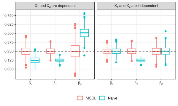
Figure 1: Boxplots of regression coefficients estimates under (M1) with $X_{1}$ and $X_{2}$ dependent (left panel) and those under a revised version of (M1) with $X_{1}$ and $X_{2}$ independent (right panel). The two boxes associated with each parameter correspond to two estimators (from left to right): the MCCL estimator (red box) and the naive estimator (cyan box).

Table 2 presents the average of standard deviation estimation of each parameter in $\Omega$ based on (12) across 1000 Monte Carlo replicates from (M1) with $n=200$. The Monte Carlo standard deviation of each parameter estimate in $\Omega$ is used as a reference/gold standard in this table. The proximity of the standard deviation estimate with the reference shown in the table suggests that the sandwich variance estimator in (12) provides reliable estimation for the variance of the MCCL estimator. This settles the second issue.

Table 2: Averages of standard deviation estimates, $\widehat{\text{s.d.}}$, and empirical standard deviation, s.d., across $1000$ Monte Carlo replicates from (M1) with $\sigma^{2}_{u}=1.2$ and $n=200$. Numbers in parentheses are Monte Carlo standard errors associated with the Monte Carlo means.

	$\beta_{0}$		$\beta_{1}$		$\beta_{2}$		$m$
	$\widehat{\text{s.d.}}$	s.d.	$\widehat{\text{ s.d. }}$	s.d.	$\widehat{\text{s.d.}}$	s.d.	$\widehat{\text{s.d.}}$	s.d.
MCCL	0.19 (0.03)	0.19	0.13 (0.03)	0.13	0.32 (0.06)	0.32	0.48 (0.07)	0.51
Naive	0.16 (0.02)	0.17	0.09 (0.01)	0.09	0.26 (0.03)	0.26	0.47 (0.05)	0.48

The third issue concerns the normality assumption on measurement error in the development of the Monte Carlo corrected score method. To assess the robustness of the MCCL estimator to this normality assumption, we revise (M1) by letting $U_{j,k}\sim\mbox{Laplace}(0,0.5^{1/2})$ instead and set $n=200$. Table 3 provides summary statistics of parameter estimates as those shown in Table 1 under this revised setting. As one can see from Table 3, despite the violation of the normality assumption on $U$, the MCCL estimates remain close to the truth and significantly outperform the naive estimates. This robustness feature of the Monte Carlo corrected score method is also noted and explained in Novick and Stefanski [2002].

Table 3: Medians of MCCL estimates and medians of naive estimates across $1000$ Monte Carlo replicates generated according to (M1) with $U_{j,k}\sim\mbox{Laplace}(0,0.5^{1/2})$ and $n=200$. The number in parentheses following each median is the interquartile range of the 1000 realizations of an estimator.

	$\beta_{0}$	$\beta_{1}$	$\beta_{2}$	$m$
MCCL	0.24 (0.18)	0.24 (0.17)	0.25 (0.27)	3.08 (0.64)
Naive	0.12 (0.20)	0.13 (0.10)	0.48 (0.32)	3.05 (0.60)

5.3 Performance of the model diagnostic method

Using 5000 Monte Carlo replicates from (M1) with $\sigma_{u}^{2}=1.2$ at each sample size level in $n=100$, 200, 500, 1000, we implement the bootstrap algorithm related in Section 4 with $M=300$ bootstrap samples to obtain estimated $p$-values associated with the test statistic $\tilde{Q}(\hat{}\mbox{\boldmath$\Omega$};\mathcal{D}^{*})$. We then record the proportion of replicates, across 5000 replicates, that lead to rejection of the null hypothesis of no model misspecification at various nominal levels. This rejection rate can be viewed as an empirical size of the test at a pre-specified significance level. Figure 2 depicts this rejection rate versus the significance level, from which one can see that the size of the test is well controlled by the bootstrap procedure over a wide range of nominal levels.

Figure 2: Rejection rates associated with the score-based diagnostic test across 5000 Monte Carlo replicates from (M1) versus the nominal level of the test. Black dashed lines are the $45^{\circ}$ reference lines.

Table 4 presents rejection rates of the model diagnostic method in the presence of different forms of model misspecification that occur when fitting data generated according to (M2)–(M4) while assuming a beta modal regression model specified in (M1). As one can see in Table 4, the proposed score-based test has moderate power to detect a misspecified form of the linear predictor, with the power steadily increasing as $n$ increases, and is especially powerful in detecting violation of the distributional assumption on $Y$ given covariates; but the test is less sensitive to link misspecification. Low power of most goodness-of-fit tests to detect link misspecification have been reported in the context of generalized linear models [e.g., Hosmer et al., 1997]. Given these reported findings in the literature, the low power observed under design (M3) may not be surprising, especially with the high similarity of the logit link in the assumed model with the probit link in the true model in (M3).

Table 4: Rejection rates of the score-based diagnostic test resulting from 300 Monte Carlo replicates in the presence of four types of model misspecification in (M2)–(M4)

Model	$n=200$	$n=300$	$n=400$	$n=500$
(M2)	0.277	0.417	0.557	0.600
(M3)	0.100	0.107	0.143	0.123
(M4)	0.997	1.000	0.993	1.000

6 Real-life data application

In this section, we analyze data arising from two different applications where a covariate of interest cannot be observed directly. Besides dealing with scientific questions in relevant fields, these applications provide opportunities for us to address some practical issues one faces when implementing the proposed estimation method and diagnostic method not discussed in the simulation study.

6.1 Application to dietary data

Food Frequency Questionnaire (FFQ) is a convenient and inexpensive dietary assessment instrument in epidemiologic studies. To study the association between an individual’s FFQ intake and his/her long-term usual intake as the univariate covariate $X$, we analyze a dietary data set from Women’s Interview Survey of Health [Carroll et al., 1997]. The data set contains 271 females’ FFQ intake records, measured as the percentage calories from fat, and six $24$-hour food recalls, $W_{j,k}$, for $j=1,\ldots,271$ and $k=1,\cdots,6$. Because the $j$-th subject’s long-term usual intake $X_{j}$ cannot be measured directly, a generally accepted practice in epidemiology is to use $\overline{W}_{j}=\sum_{k=1}^{6}W_{j,k}/6$ as a surrogate of $X_{j}$, for $j=1,\ldots,271$. According to the preliminary analysis in existing literature, the distribution of the FFQ intake appears to be right-skewed and potentially heavy-tailed, which motivates the consideration of a modal regression model in place of a mean regression model. Here, we assume a beta modal regression model given in (2) with $\theta(X)=1/\{1+\exp(-\beta_{0}-\beta_{1}X)\}$ for the response data $\{Y_{j}\}_{j=1}^{271}$, where $Y_{j}$ is the $j$-th subject’s FFQ intake in kilocalorie divided by 8000, a biologically plausible upper bound of daily energy intakes for a general population.

We obtain the MCCL estimate of $\mbox{\boldmath$\Omega$}=(\beta_{0},\beta_{1},\log m)^{\mathrm{\scriptscriptstyle T}}$ according to (11), and also carry out regression analysis that ignores measurement error to obtain a naive maximum likelihood estimate of $\Omega$. These two sets of estimates are given in Table 5. The covariate effect associated with the long-term intake suggested by the naive estimate is substantially weaker than that indicated by the MCCL estimate, implying potentially significant attenuation on the covariate effect due to measurement error in the former, whereas the latter corrects for this attenuation. Figure 3 depicts the estimated regression functions $\hat{\theta}(x)$ resulting from these two methods, imposed on the scaled response data versus the surrogate covariate data. This pictorial contrast between the two estimated regression functions shows that the proposed method is able to capture the underlying positive non-linear covariate effect that is partially concealed or weakened by the naive method. Finally, applying the proposed diagnostic method to this data set with $M=300$ bootstrap samples yields an estimated $p$-value of 0.61. We thus conclude lack of sufficient data evidence to indicate the assumed beta modal regression model inadequate for this application.

Table 5: Estimates of parameters in the beta modal regression model applied to the dietary data, along with the corresponding estimated standard errors in parentheses

Method	$\beta_{0}$	$\beta_{1}$	$\log m$
MCCL	$-1.569$ (0.049)	1.056 (0.420)	3.298 (0.345)
Naive	$-1.581$ (0.041)	0.270 (0.058)	2.979 (0.094)

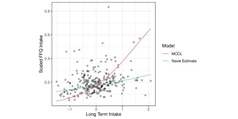
Figure 3: Estimated conditional mode functions for the dietary data based on the MCCL estimate (red solid line) and the naive estimate (cyan dashed line), respectively. Observed covariate data $\{\overline{W}_{j}\}_{j=1}^{271}$ are treated as surrogates of long-term usual intakes in the scatter plot of the observed data (solid dots).

6.2 Application to Alzheimer’s disease data

Medical researchers have long recognized that cerebral atrophy is associated with dementia, and extensive research have been conducted to understand the association between volumetric changes of different brain regions with the severity of dementia. Abundant data collected from this line of research are available in the Alzheimer’s Disease Neuroimaging Initiative (ADNI) database (http://adni.loni.usc.edu/). Zhou and Huang [2020] analyzed a data set relating to 245 individuals diagnosed with mild cognitive impairment from this database. The goal is to study roles that an individual’s volumetric measure of entorhinal cortex (ERC) and that of hippocampus (HPC) play in predicting one’s risk of developing Alzheimer’s disease. An individual’s test score from the Alzheimer’s disease assessment scale, known as ADAS-11, at month 12 since entering the ADNI cohort is used to assess one’s severity of cognitive impairment. Covariates of interest are the volumetric change in ERC (ERC.change) and that in HPC (HPC.change) at month 12 compared to the baseline measures collected at month 6. Assuming these volumetric measures are observed precisely, Zhou and Huang [2020] fitted the data to the beta modal regression model for the response $Y$ defined as an individual’s ADAS-11 score divided by a perfect score of 70, with the log-log link in the mode function, $\theta(\mathbf{X})=\exp\{-\exp(-\beta_{0}-\beta_{1}\times\text{ERC.change}-\beta_{2}\times\text{HPC.change})\}$, and showed that it provides a better fit for the data compared to the beta mean regression model proposed by Ferrari and Cribari-Neto [2004].

In reality, measuring ERC volume is challenging because of lateral border discrimination from the perirhinal cortex [Price et al., 2010], and the accuracy of HPC measurements is also in question [Maclaren et al., 2014]. It is thus more sensible to view the observed volumetric change of ERC or that of HPC as a noisy surrogate of the actual amount of change. Despite of which covariate is viewed as error-prone, the current data present some challenges due to the lack of replicate measures for an individual’s true covariate value, and thus the estimation methods proposed in Section 3 are not applicable. For example, in (10), the term multiplying the imaginary unit $i$ is equal to zero now with the number of replicates $n_{j}=1$, making the “corrected" log-likelihood the same as the naive log-likelihood. A quick fix to the problem is to invoke a similar strategy of correcting naive scores to account for measurement error as discussed in Novick and Stefanski [2002]. Following this strategy, a corrected log-likelihood evaluated at the $j$-th data point to use in place of (10) is

$$\tilde{\ell}(\mbox{\boldmath$\Omega$};Y_{j},\mathbf{W}_{j},\tilde{\mathbf{Z}}_{j})=\frac{1}{B}\sum_{b=1}^{B}\text{Re}\{\ell(\mbox{\boldmath$\Omega$};Y_{j},\mathbf{W}_{j}+i\mbox{\boldmath$\Sigma$}_{u}^{1/2}\mathbf{Z}_{j,b})\},$$ (18)

where $\tilde{\mathbf{Z}}_{j}=\{\mathbf{Z}_{j,b}\}_{b=1}^{B}$, for $j=1,\ldots,n$, and $\{\mathbf{Z}_{j,b},b=1,\ldots,B\}_{j=1}^{n}$ are independent $p$-dimensional normal random vectors with mean zero and variance-covariance as an identity matrix, which accommodates multiple error-prone covariates in $\mathbf{X}$ by letting $\mathbf{W}_{j}$ be a $p$-dimensional multivariate surrogate of $\mathbf{X}_{j}$, contaminated by a multivariate normal measurement error $\mathbf{U}_{j}$ with variance-covariance matrix $\mbox{\boldmath$\Sigma$}_{u}$. By setting all entries in $\mbox{\boldmath$\Sigma$}_{u}$ at zero except for the first diagonal entry gives rise to the case considered in the majority of this article with only $X_{1}$ prone to error. Certainly, not having replicate measures still creates an obstacle to implementing this strategy due to its dependence on $\mbox{\boldmath$\Sigma$}_{u}$ that cannot be estimated without replicate measures of a true multivariate covariate value or other external validation data. A well-accepted practice among statisticians in similar situations is to carry out sensitivity analysis where one analyzes the data under different assumptions for the parameter, such as $\mbox{\boldmath$\Sigma$}_{u}$ in our case, that one lacks data information to infer. If one obtains drastically different inference results when assuming different values for $\mbox{\boldmath$\Sigma$}_{u}$, including a matrix of zeros corresponding to naive estimation that ignores measurement error, then one may recommend to exercise caution when interpreting results from an inference procedure that assumes error-free covariates.

For illustration purposes, we assume in the sensitivity analysis four values for $\mbox{\boldmath$\Sigma$}_{u}$ listed in Table 6, where inference results for model parameters under each assumed $\mbox{\boldmath$\Sigma$}_{u}$ are provided. According to Table 6, all four rounds of regression analyses lead to the conclusion that the volumetric change of ERC is an influential predictor for the severity of cognitive impairment, even though the magnitude of the estimated covariate effect is sensitive to the assumed error variance associated this covariate. In particular, when assuming imprecise measurements for ERC.change, the revised MCCL method that employs the corrected log-likelihood in (18) with $B=1000$ produces results indicating a much stronger association than the naive analysis. By comparison, the magnitude of the estimate for the HPC.change effect is less sensitive to the assumed $\mbox{\boldmath$\Sigma$}_{u}$, but its statistical significance is noticeably affected by it. For example, one would conclude a moderately significant covariate effect of HPC.change based on the naive analysis assuming error-free covariates, but claim a highly significant, or moderately significant, or nonsignificant HPC.change effect depending on which covariate(s) one assumes to be error-prone and the severity of error contamination. This phenomenon is a reminiscence of an observation made in Figure 1, and may suggest that ERC.change and HPC.change are correlated. In fact, measurements of ERC and HPC via magnetic resonance imaging are known to be highly correlated with observed clinical alterations in patients suffering mild cognitive impairment or at dementia phases of Alzheimer’s disease [Desikan et al., 2010, Jack et al., 2013, Varon et al., 2014].

Table 6: Sensitivity analysis using the ADNI data for the beta modal regression with the log-log link. Numbers in parentheses are estimated standard errors. Numbers in square brackets are $p$-values associated with covariate effects.

$\mbox{\boldmath$\Sigma$}_{u}$	$\beta_{0}$	$\beta_{1}$ (ERC.change)	$\beta_{2}$ (HPC.change)	$\log m$
$\begin{bmatrix}0&0\\ 0&0\end{bmatrix}$	$-0.69$ (0.03)	$-0.12$ (0.05)	$-0.22$ (0.11)	2.78 (0.15)
		[0.007]	[0.054]
$\begin{bmatrix}0.16&0\\ 0&0\end{bmatrix}$	$-0.83$ (0.09)	$-2.47$ (0.00)	$-0.30$ (1.03)	2.40 (0.02)
		[0.000]	[0.773]
$\begin{bmatrix}0&0\\ 0&0.0225\end{bmatrix}$	$-0.71$ (0.03)	$-0.11$ (0.05)	$-0.46$ (0.27)	2.80 (0.16)
		[0.013]	[0.084]
$\begin{bmatrix}0.16&0\\ 0&0.0225\end{bmatrix}$	$-0.81$ (0.03)	$-2.45$ (0.00)	$-0.87$ (0.06)	3.94 (0.01)
		[0.000]	[0.000]

In conclusion, results from the sensitivity analysis suggest that volumetric measures of different brain regions are likely to be subject to measurement error, and statistical analyses under the assumption of precisely measured covariates should be interpreted with caution. If replicate data are available for covariates of interest, the MCCL method can provide more reliable inference. Lastly, even though one can mimic (18) to construct a corrected score in place of $\tilde{\mathbf{S}}(\mbox{\boldmath$\Omega$};Y_{j},\widetilde{W}_{j},\widetilde{T}_{j},\mathbf{X}_{-1,j})$ in (15) and then formulate the test statistic $\tilde{Q}(\hat{}\mbox{\boldmath$\Omega$};\mathcal{D}^{*})$ for model diagnostics, the dependence of the revised score on the unknown $\mbox{\boldmath$\Sigma$}_{u}$ remains an obstacle that hinders one from using the bootstrap procedure outlined in Section 4 to assess statistical significance of the revised test statistic. Alternative diagnostic methods that do not rely on parametric bootstrap or corrected score [e.g. Huang et al., 2006] can be used to detect inadequate assumptions imposed on the primary regression model.

7 Discussion

We propose an inference procedure based on the idea of corrected score that falls in the framework of $M$-estimation for modal regression with an error-prone covariate. Even though in this article we focus on the beta modal regression model as the primary regression model, the proposed MCCL method is applicable in other parametric modal regression models, such as the gamma modal regression models for non-negative responses proposed by Aristodemou [2014] and Bourguignon et al. [2020]. A Python package for implementing the proposed methods for beta modal regression with errors-in-covariate is available at https://pypi.org/project/pybetareg/. All computer programs used in this paper is available at https://github.com/rh8liuqy/Modal_regression_with_measurement_error.

To accommodate situations without replicate measures of the true covariate or settings with multiple error-prone covariates, the MCCL method can be easily revised as demonstrated in Section 6.2, although one needs to specify the variance (or the variance-covariance matrix) of the (vector-valued) measurement error if one lacks replicate data or external validation data to estimate it.

Focusing on the current beta modal regression models, some extensions are worthy of further investigation, such as a zero-inflated beta modal regression model to fit disease prevalence data especially suitable for rare diseases. Another follow-up research direction is variable selection based on a parametric modal regression model with or without measurement error contamination in covariates.

References

- Chacón [2020] José E. Chacón. The modal age of statistics. International Statistical Review, 88(1):122–141, 2020. doi:10.1111/insr.12340.
- Sager and Thisted [1982] Thomas W. Sager and Ronald A. Thisted. Maximum likelihood estimation of isotonic modal regression. The Annals of Statistics, 10(3):690–707, 1982. doi:10.1214/aos/1176345865.
- Lee [1989] Myoung-Jae Lee. Mode regression. Journal of Econometrics, 42(3):337–349, 1989. doi:10.1016/0304-4076(89)90057-2.
- Lee [1993] Myoung-Jae Lee. Quadratic mode regression. Journal of Econometrics, 57(1-3):1–19, 1993. doi:10.1016/0304-4076(93)90056-b.
- Yao and Li [2013] Weixin Yao and Longhai Li. A new regression model: Modal linear regression. Scandinavian Journal of Statistics, 41(3):656–671, 2013. doi:10.1111/sjos.12054.
- Chen et al. [2016] Yen-Chi Chen, Christopher R. Genovese, Ryan J. Tibshirani, and Larry Wasserman. Nonparametric modal regression. The Annals of Statistics, 44(2):489–514, 2016. doi:10.1214/15-aos1373.
- Aristodemou [2014] Katerina Aristodemou. New regression methods for measures of central tendency. PhD thesis, Brunel University, 2014.
- Bourguignon et al. [2020] Marcelo Bourguignon, Jeremias Leão, and Diego I Gallardo. Parametric modal regression with varying precision. Biometrical Journal, 62(1):202–220, 2020.
- Zhou and Huang [2020] Haiming Zhou and Xianzheng Huang. Parametric mode regression for bounded responses. Biometrical Journal, 62(7):1791–1809, 2020. doi:10.1002/bimj.202000039.
- Zhou and Huang [2022] Haiming Zhou and Xianzheng Huang. Bayesian beta regression for bounded responses with unknown supports. Computational Statistics & Data Analysis, 167:107345, 2022.
- Carroll et al. [2006] Raymond J. Carroll, David Ruppert, Leonard A. Stefanski, and Ciprian M. Crainiceanu. Measurement Error in Nonlinear Models. Chapman and Hall/CRC, 2006. doi:10.1201/9781420010138.
- Fuller [2009] Wayne A Fuller. Measurement Error Models. John Wiley & Sons, 2009.
- Buonaccorsi [2010] John P. Buonaccorsi. Measurement Error: Models, Methods, and Applications. Chapman and Hall/CRC, 2010.
- Yi [2017] Grace Y. Yi. Statistical Analysis with Measurement Error or Misclassification. Springer New York, 2017. doi:10.1007/978-1-4939-6640-0.
- He and Liang [2000] Xuming He and Hua Liang. Quantile regression estimates for a class of linear and partially linear errors-in-variables models. Statistica Sinica, 10(1):129–140, 2000.
- Wei and Carroll [2009] Ying Wei and Raymond J Carroll. Quantile regression with measurement error. Journal of the American Statistical Association, 104(487):1129–1143, 2009.
- Wang et al. [2012] Huixia Judy Wang, Leonard A Stefanski, and Zhongyi Zhu. Corrected-loss estimation for quantile regression with covariate measurement errors. Biometrika, 99(2):405, 2012.
- Zhou and Huang [2016] Haiming Zhou and Xianzheng Huang. Nonparametric modal regression in the presence of measurement error. Electronic Journal of Statistics, 10(2), 2016. doi:10.1214/16-ejs1210.
- Li and Huang [2019] Xiang Li and Xianzheng Huang. Linear mode regression with covariate measurement error. Canadian Journal of Statistics, 47(2), 2019. doi:10.1002/cjs.11492.
- Shi et al. [2021] Jianhong Shi, Yujing Zhang, Ping Yu, and Weixing Song. SIMEX estimation in parametric modal regression with measurement error. Computational Statistics & Data Analysis, 157:107158, 2021. doi:10.1016/j.csda.2020.107158.
- Nakamura [1990] Tsuyoshi Nakamura. Corrected score function for errors-in-variables models: Methodology and application to generalized linear models. Biometrika, 77(1), 1990. doi:10.2307/2336055.
- Stefanski et al. [2005] Leonard A. Stefanski, Steven J. Novick, and Viswanath Devanarayan. Estimating a nonlinear function of a normal mean. Biometrika, 92(3):732–736, 2005. doi:10.1093/biomet/92.3.732.
- White [1982] Halbert White. Maximum likelihood estimation of misspecified models. Econometrica: Journal of the econometric society, pages 1–25, 1982.
- Boos and Stefanski [2013] Dennis D Boos and Leonard A Stefanski. Essential statistical inference: theory and methods, volume 591. Springer, 2013.
- Buonaccorsi et al. [2018] John P. Buonaccorsi, Giovanni Romeo, and Magne Thoresen. Model-based bootstrapping when correcting for measurement error with application to logistic regression. Biometrics, 74(1):135–144, 2018. doi:10.1111/biom.12730.
- Novick and Stefanski [2002] Steven J Novick and Leonard A Stefanski. Corrected score estimation via complex variable simulation extrapolation. Journal of the American Statistical Association, 97(458):472–481, 2002. doi:10.1198/016214502760047005.
- Hosmer et al. [1997] David W Hosmer, Trina Hosmer, Saskia Le Cessie, and Stanley Lemeshow. A comparison of goodness-of-fit tests for the logistic regression model. Statistics in medicine, 16(9):965–980, 1997.
- Carroll et al. [1997] Raymond J. Carroll, Laurence Freedman, and David Pee. Design aspects of calibration studies in nutrition, with analysis of missing data in linear measurement error models. Biometrics, 53(4), 1997. doi:10.2307/2533510.
- Ferrari and Cribari-Neto [2004] Silvia Ferrari and Francisco Cribari-Neto. Beta regression for modelling rates and proportions. Journal of Applied Statistics, 31(7):799–815, 2004. doi:10.1002/bimj.202000039.
- Price et al. [2010] C.C. Price, M.F. Wood, C.M. Leonard, S. Towler, J. Ward, H. Montijo, I. Kellison, D. Bowers, T. Monk, J.C. Newcomer, and et al. Entorhinal cortex volume in older adults: Reliability and validity considerations for three published measurement protocols. Journal of the International Neuropsychological Society, 16:846–855, 2010. doi:10.1017/S135561771000072X.
- Maclaren et al. [2014] Julian Maclaren, Zhaoying Han, Sjoerd B Vos, Nancy Fischbein, and Roland Bammer. Reliability of brain volume measurements: A test-retest dataset. Scientific Data, 1(1), 2014. doi:10.1038/sdata.2014.37.
- Desikan et al. [2010] Rahul S. Desikan, Howard J. Cabral, Fabio Settecase, Christopher P. Hess, William P. Dillon, Christine M. Glastonbury, Michael W. Weiner, Nicholas J. Schmansky, David H. Salat, and Bruce Fischl. Automated mri measures predict progression to alzheimer’s disease. Neurobiology of Aging, 31(8), 2010. doi:10.1016/j.neurobiolaging.2010.04.023.
- Jack et al. [2013] Clifford R Jack, David S Knopman, William J Jagust, Ronald C Petersen, Michael W Weiner, Paul S Aisen, Leslie M Shaw, Prashanthi Vemuri, Heather J Wiste, Stephen D Weigand, Timothy G Lesnick, Vernon S Pankratz, Michael C Donohue, and John Q Trojanowski. Tracking pathophysiological processes in alzheimer’s disease: an updated hypothetical model of dynamic biomarkers. The Lancet Neurology, 12(2):207–216, 2013. doi:10.1016/s1474-4422(12)70291-0.
- Varon et al. [2014] Daniel Varon, Warren Barker, David Loewenstein, Maria Greig, Adriana Bohorquez, Isael Santos, Qian Shen, Molly Harper, Tatiana Vallejo-Luces, and Ranjan Duara and. Visual rating and volumetric measurement of medial temporal atrophy in the alzheimer’s disease neuroimaging initiative (ADNI) cohort: baseline diagnosis and the prediction of MCI outcome. International Journal of Geriatric Psychiatry, 30(2):192–200, 2014. doi:10.1002/gps.4126.
- Huang et al. [2006] Xianzheng Huang, Leonard A Stefanski, and Marie Davidian. Latent-model robustness in structural measurement error models. Biometrika, 93(1):53–64, 2006.