Numerical simulation for the motions of nonautonomous solitary waves of a variable-coefficient forced Burgers equation via the lattice Boltzmann method

Abstract

The lattice Boltzmann method (LBM) for the variable-coefficient forced Burgers equation (vc-FBE) is studied by choosing the equilibrium distribution and compensatory functions properly. In our model, the vc-FBE is correctly recovered via the Chapman-Enskog analysis. We numerically investigate the dynamic characteristics of solitons caused by the dispersive and external-force terms. Four numerical examples are given, which align well with the theoretical solutions. Our research proves that LBM is a satisfactory and efficient method for nonlinear evolution equations with variable coefficients.

Keywords: The variable-coefficient forced Burgers equation; Chapman-Enskog expansion; External-force term; Lattice Boltzmann method

1 Introduction

The lattice Boltzmann method (LBM) has drawn broad attention in simulations of fluid flows in different mathematical and physical fields [1]. As one of the most popular models via the LBM, the lattice Bhatnagar-Gross-Krook one has been applied in various fields successfully [2]. Compared with other traditional simulation approaches (for instance, the finite difference [3], Galerkin [4], Chebyshev spectral [5], finite element [6], heat balance integral [7], variational iteration [8] and decomposition methods [9]), the LBM has such advantages as the parallel calculation, algorithmic simplicity and easy-to-handle of marginal conditions. Based on the successive Boltzmann equation, the macroscopic variable is derived easily and the macroscopic equation is also recovered correctly under the assistance of Chapman-Enskog expansion [10].

Recently, the LBM has been employed in certain nonlinear evolution equations (NLEEs), including the Burgers [11], Korteweg-de Vries and Burgers [12], improved Korteweg-de Vries [13] and convection-diffusion equations [14], to name a few. Nevertheless, such studies mainly focused on the constant-coefficient cases but little involved the variable-coefficient ones, especially for the nonlinear models with variable external-force term. External-force coefficient can depict the time evolution of varying interface contour in different reaction-diffusion models [15]. Indeed, Ref. [16] shows that the nonautonomous solitons can show more dynamic characteristics, which do not appear in the constant-coefficient NLEEs [17, 18, 19, 20].

In this work, we work over the variable-coefficient forced Burgers equation (vc-FBE) as follows [21]

$$u_{t}+a(x,t)uu_{x}+b(x,t)u_{xx}-m(x,t)=0,$$ (1)

where the function $u(x,t)$ represents the fluid velocity field, and $a(x,t)$, $b(x,t)$ and $m(x,t)$ denote the nonlinear, dispersive and external-force coefficients, respectively. Xu $et$ $al$. have presented the multi-soliton solutions of Eq. (1) through the generalized Hopf-Cole transform [15]. Gao $et$ $al$. [21] have achieved several kinds of exact soliton-like solutions of Eq. (1). When $a(x,t)$ = 1, $b(x,t)=-\frac{1}{Re}$ and $m(x,t)$ = 0, Eq. (1) can be transformed into the Burgers equation [22]

$$u_{t}+uu_{x}-\frac{u_{xx}}{Re}=0,$$ (2)

where $Re$ stands for the Reynolds number describing the coefficient of kinematic viscosity $v$ ($v=\frac{1}{Re}$). Refs. [23, 24, 25] have numerically investigated the Burgers equation through the LBM. However, to the best of our knowledge, few studies focused on the Burgers equation with the variable and external-force coefficients based on the LBM.

In this work, by using the LBM, we will show the dynamics of the nonautonomous solitons described by Eq. (1). The rest part of this article is listed as below: in Section 2, the lattice Boltzmann model will be proposed; in Section 3, the accurateness and durability of the proposed model will be verified by four numerical experiments; our consequences will be given in Section 4.

2 The lattice Boltzmann model

In this section, we choose the D1Q3 velocity model in which the discrete velocities can be written as: $\{c_{0},c_{1},c_{2}\}=\{0,c,-c\}$. $c$ is a constant and $c=\Delta x/\Delta t$, in which $\Delta t$ and $\Delta x$ are the lattice time and space steps, singly. The evolution equation described by the density distribution function is shown below.

$$f_{i}(x+c_{i}\Delta t,t+\Delta t)=f_{i}(x,t)-\frac{1}{\tau}(f_{i}(x,t)-f_{i}^{eq}(x,t))+h_{i}(x,t)\Delta t+\frac{m(x,t)}{3}\Delta t,$$ (3)

in which $f_{i}(x,t)$ and $f_{i}^{eq}(x,t)$ are defined as the density distribution and equilibrium distribution functions and $\tau$ is the dimensionless relaxation time. $h_{i}(x,t)$ is a compensatory function added in Eq. (3)

$$h_{i}(x,t)=\lambda_{i}u^{2}.$$ (4)

To generate the equilibrium distribution function, Taylor expansion is applied to Eq. (3) with the terms expanded up to O$(\Delta t^{3})$

$$\Delta t\frac{\partial f_{i}(x,t)}{\partial t}+\Delta t\frac{\partial(c_{i}f_{i}(x,t))}{\partial x}+\frac{1}{2}\Delta t^{2}\frac{\partial^{2}f_{i}(x,t)}{\partial t^{2}}+\Delta t\frac{\partial^{2}(c_{i}f_{i}(x,t))}{\partial x\partial t}+\frac{1}{2}\Delta t^{2}\frac{\partial^{2}(c_{i}^{2}f_{i}(x,t))}{\partial x^{2}}\vspace{1ex}$$ (5)

$$=-\frac{1}{\tau}(f_{i}(x,t)-f_{i}^{eq}(x,t))+\Delta th_{i}(x,t)+\frac{\Delta tm(x,t)}{3}+{\rm O}(\Delta t^{3}).$$

Then, we give the following expressions via the Chapman-Enskog expansion

$$f_{i}(x,t)=\sum_{n=0}^{\infty}\epsilon^{n}f_{i}^{(n)}(x,t)=\epsilon^{0}f_{i}^{\left(0\right)}(x,t)+\epsilon^{1}f_{i}^{\left(1\right)}(x,t)+\epsilon^{2}f_{i}^{\left(2\right)}(x,t)+...~{},$$ (6)

$$\frac{\partial}{\partial t}=\epsilon\frac{\partial}{\partial t_{1}},m(x,t)=\epsilon m_{1}(x,t).$$

Let $\epsilon$=$\Delta t$, by inserting Eq. (6) into Eq. (5), we can obtain a serial of differential equations

$$\rm{O} (\Delta t^{0}):f_{i}^{\left(0\right)}(x,t)-f_{i}^{\left({eq}\right)}(x,t)=0,$$ (7)

$$\rm{O} (\Delta t^{1}):\frac{\partial}{{\partial x}}\left({{c_{i}}f_{i}^{\left(0\right)}(x,t)}\right)+\frac{1}{\tau}f_{i}^{\left(1\right)}(x,t)-h_{i}(x,t)=0,$$ (8)

$$\rm{O} (\Delta t^{2}):\frac{{\partial f_{i}^{\left(0\right)}(x,t)}}{{\partial{t_{1}}}}+\frac{\partial}{{\partial x}}\left({{c_{i}}f_{i}^{\left(1\right)}(x,t)}\right)+\frac{1}{2}\frac{{{\partial^{2}}}}{{\partial{x^{2}}}}\left({c_{i}^{2}f_{i}^{\left(0\right)}(x,t)}\right)+\frac{1}{\tau}f_{i}^{\left(2\right)}(x,t)-\frac{{{m_{1}}\left({x,t}\right)}}{3}=0.$$ (9)

Similar to the general lattice Boltzmann model, the macroscopic variable $u$ is given by

$$u=\sum\limits_{i}{f_{i}}(x,t).$$ (10)

The equilibrium distribution function should suit the following constraint via the conservative law

$$u=\sum\limits_{i}{f_{i}^{\left(0\right)}(x,t)}=\sum\limits_{i}{f_{i}^{\left({eq}\right)}(x,t)}.$$ (11)

Based on Eq. (11), we have

$$\sum\limits_{i}{f_{i}^{\left(n\right)}(x,t)}=0,\left({n>0}\right).$$ (12)

Considering the structure of Eq. (1), we have to take other constraints on the equilibrium distribution and compensatory functions

$$\sum\limits_{i}{c_{i}f_{i}^{\left(0\right)}(x,t)}={F_{1}},~{}\sum\limits_{i}{c_{i}^{2}f_{i}^{\left(0\right)}(x,t)}={F_{2}},~{}\sum\limits_{i}{{h_{i}}(x,t)={H_{0}}},~{}\sum\limits_{i}{{c_{i}}{h_{i}}(x,t)={H_{1}}}.$$ (13)

Through Eq. (8) and noting Eq. (13), we obtain

$$\sum\limits_{i}{{c_{i}}f_{i}^{(1)}(x,t)}=\tau\sum\limits_{i}{{c_{i}}{h_{i}}(x,t)-\tau\frac{\partial}{{\partial x}}}\sum\limits_{i}{c_{i}^{2}f_{i}^{(0)}(x,t)}=\tau{H_{1}}-\tau\frac{\partial F_{2}}{\partial x}.$$ (14)

By using the summation of Eq. (8) over $i$, and considering Eqs. (11) and (13), we get

$$\frac{{\partial{F_{1}}}}{{\partial x}}={H_{0}}.$$ (15)

Similarly, using the summation of Eq. (9) over $i$, and noting Eqs. (11), (12), (13) and (14), we have

$$\frac{{\partial u}}{{\partial{t_{1}}}}+(\frac{1}{2}-\tau)\frac{{{\partial^{2}}{F_{2}}}}{{\partial{x^{2}}}}+\tau\frac{{\partial{H_{1}}}}{{\partial x}}={m_{1}}(x,t).$$ (16)

In terms of the structure of $\Delta t$$\times$(15)+$\Delta t^{2}$$\times$(16), Eq. (1) can be converted into

$$\frac{{\partial u}}{{\partial t}}+\Delta t\tau\frac{{\partial{H_{1}}}}{{\partial x}}+\frac{{\partial{F_{1}}}}{{\partial x}}+(\frac{1}{2}-\tau)\Delta t\frac{{{\partial^{2}}{F_{2}}}}{{\partial{x^{2}}}}=m(x,t)+{H_{0}}.$$ (17)

Comparing Eq. (17) with Eq. (1), we take

$${F_{1}}=0,~{}{F_{2}}=c^{2}\eta u,~{}{H_{0}}=0,~{}{H_{1}}=c{\lambda}{u^{2}}.$$ (18)

Applying Eq. (18) to Eq. (17), we finally have the following equation

$${u_{t}}+2\tau\Delta tc\lambda u{u_{x}}+(\frac{1}{2}-\tau)\Delta t{c^{2}}\eta u_{xx}=m(x,t).$$ (19)

Observing the forms of Eqs. (19) and (1), we get

$$\begin{array}[]{l}a(x,t)=2\tau\Delta tc\lambda,~{}b(x,t)=(\frac{1}{2}-\tau)\Delta t{c^{2}}\eta.\end{array}$$ (20)

Combining Eq. (10) and the first two terms of Eq. (13), the equilibrium distribution function is written as

$$f_{i}^{(eq)}(x,t)=\begin{cases}~{}(1-\eta)u,&\text{$i$=0},\\ \quad~{}~{}\frac{\eta u}{2},&\text{$i$=1},\\ \quad~{}~{}\frac{\eta u}{2},&\text{$i$=2}.\end{cases}$$

Combining Eqs. (4), (18) and the last two terms of Eq. (13), the compensatory function $h_{i}(x,t)$ can be solved. To simplify the simulation without losing generality, we take only one case for $h_{i}(x,t)$

$$h_{i}(x,t)=\begin{cases}~{}~{}\frac{1}{3}\lambda u^{2},&\text{$i$=0},\\ ~{}~{}\frac{1}{3}\lambda u^{2},&\text{$i$=1},\\ -\frac{2}{3}\lambda u^{2},&\text{$i$=2}.\end{cases}$$

3 Numerical results

Hereby, we give four computational experiments for Eq. (1), the theoretical ones of which has already been presented in Ref. [21]. By comparing these two types of results, we can confirm the accuracy of the presented model. The velocity $u(x,t)$ is determined by incipient condition and the distribution function $f_{i}(x,t)$ is first initialized to be $f_{i}^{(0)}(x,t)$. In addition, the absolute error (AE) and global relative error (GRE) are presented to test the effectiveness of this model, which are defined as

$$\small{\rm AE}=|{u^{\dagger}}({x_{i}},t)-u({x_{i}},t)|,~{}{\rm GRE}=\frac{{\sum\limits_{i}{|{u^{\dagger}}({x_{i}},t)-u({x_{i}},t)|}}}{{\sum\limits_{i}{|{u^{\dagger}}({x_{i}},t)|}}},$$

where $u^{\dagger}(x_{i},t)$ and $u(x_{i},t)$ are the theoretical and computational solutions, respectively. In Ref. [21], the nonlinear, dispersive and external-force coefficients of Eq. (1) are given as

$$a(x,t)=\frac{xb_{1}(t)+b_{2}(t)}{p+\int b_{1}(t)[q+\int m(t)dt]dt},~{}b(x,t)=xb_{1}(t)+b_{2}(t),~{}m(x,t)=m(t).$$ (21)

The first-order theoretical solution of Eq. (1) is given by [21]

$$u(x,t)=q+\int m(t)dt+L\tanh\Bigg{[}w+\frac{Lx}{2[p+\int b_{1}(t)[q+\int m(t)dt]dt]}-\frac{L}{2}\int\frac{b_{2}(t)[q+\int m(t)dt]}{\big{[}p+\int b_{1}(t)[q+\int m(t)dt]dt\big{]}^{2}}dt\Bigg{]}.$$ (22)

Example 1. In this simulation, we take the same parameters with Ref. [21]. Here $b_{1}(t)$, $b_{2}(t)$ and $m(t)$ are set to be 0, -2 and 0. Other parameters in our model are set as $w=6$, $p=-5$, $q=10$, $L=4$, $\Delta t=0.0001$ and $\Delta x=0.01$, respectively. The simulation domain is immobilized to [0,40]. Then the theoretical solution is expressed as

$$u(x,t)=10+4\tanh(6+1.6t-0.4x).$$ (23)

Here Eq. (1) is restricted to the incipient condition

$$u(x,0)=10+4\tanh(6-0.4x),~{}0\leq x\leq 40,$$ (24)

and the marginal conditions

$$u(0,t)=14,~{}u(40,t)=6,~{}t\geq 0.$$ (25)

Fig. 1(a) shows that the velocity of the soliton doesn’t change with time [21]. Fig. 1(b) depicts that computational results align well with the theoretical ones. In detail, the GRE and relaxation time ($\tau$) of computational results are given in Tab. 1.

Tab. 1: The GRE and relaxation time ($\tau$) for computational results of Example 1

$t$	$t$=0.2	$t$=1.0	$t$=1.8
GRE	5.1826e-05	1.9123e-04	2.6970e-04
$\tau$	2.5	2.5	2.5

Example 2. Compared with the situation in Example 1, we choose the same functions and parameters except that $b_{2}(t)=-2-t^{2}$. Then the theoretical solution of this example is written as

$$u(x,t)=10+4\tanh(6+1.6t+\frac{4}{15}t^{3}-0.4x).$$ (26)

The GRE and relaxation time ($\tau$) of computational results are given in Tab. 2. In order to compare these two types of results explicitly, we give the detailed computational and theoretical results in Tab. 3. The AE shows that computational results are accurate enough. Fig. 2(a) reveals that the dispersion changes the velocity of the soliton [21]. Here we use $\Delta x$ in Fig. 2(b) to represent the change of displacement during the same time $\Delta t=0.8$. We can find that computational results describe the effect of the dispersion on the motion of the soliton pretty well ($\Delta x_{1}<\Delta x_{2}$).

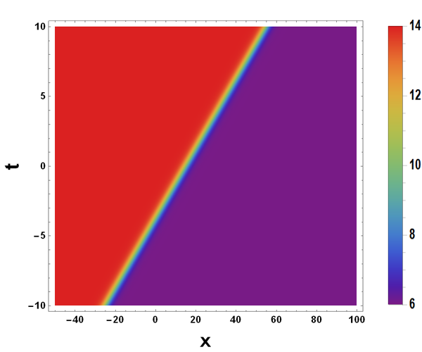
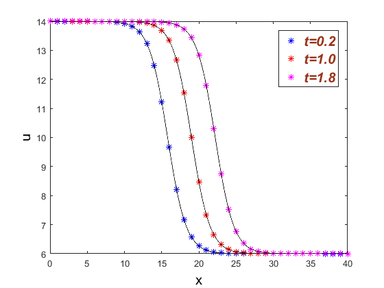
Fig. 1: (Color online) (a) Density plot of the theoretical solution (23); (b) Computational results and the theoretical solution of Example 1 at $t=0.2,1.0,1.8$. Discrete points and solid lines respectively denote the computational and theoretical solutions.

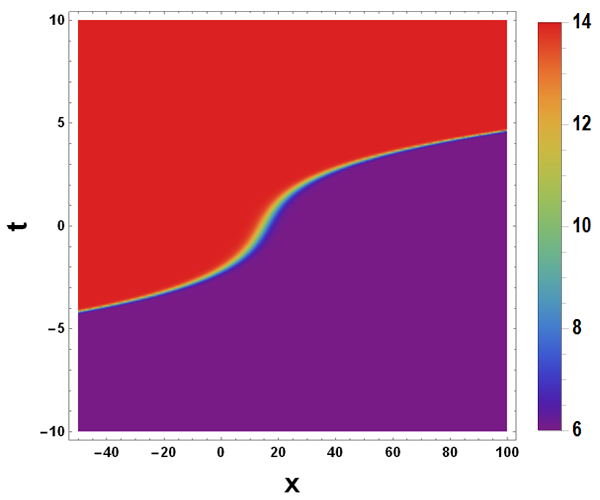
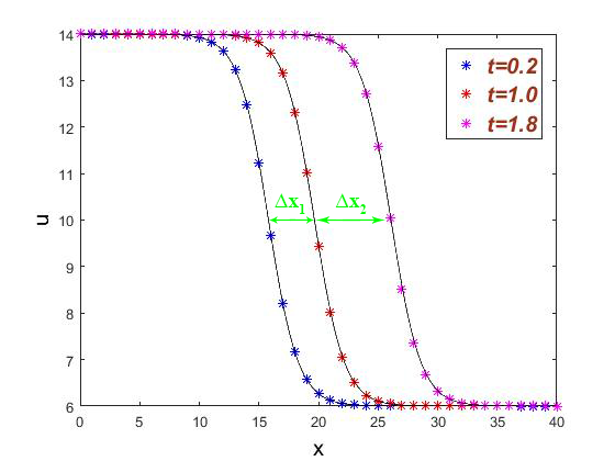
Fig. 2: (Color online) (a) Density plot of the theoretical solution (26); (b) Computational results and the theoretical solution of Example 2 at $t=0.2,1.0,1.8$. The meanings of discrete points and solid lines are the same as Fig. 1.

Tab. 2: The GRE and relaxation time ($\tau$) for computational results of Example 2

$t$	$t$=0.2	$t$=1.0	$t$=1.8
GRE	1.2185e-04	4.1204e-04	8.8659e-04
$\tau$	2.5	2.5225	2.86

Tab. 3: The comparison between the theoretical and computational results of Example 2 at $t$=0.2

$x$	theoretical results	computational results	AE
4.0	13.999367	13.999370	3.0860e-06
8.0	13.984498	13.984510	1.2332e-05
12.0	13.636275	13.636260	1.4848e-05
16.0	9.6891613	9.678672	1.0489e-02
20.0	6.2696634	6.267866	1.7974e-03
24.0	6.0113594	6.011281	7.8366e-05
28.0	6.0004637	6.000460	3.6643e-06
32.0	6.0000189	6.000019	9.8970e-08
36.0	6.0000008	6.000001	2.2955e-07

Example 3. In this example, we select the same functions and parameters with Example 1 except that $m(t)=\frac{1}{2}\sin(t+5)$. Therefore, the expression of the theoretical solution is as follows

$$u(x,t)=10-\frac{1}{2}\cos(5+t)+4\tanh\big{[}6+1.6t-0.4x-\sin(5+t)\big{]}.$$ (27)

The GRE and relaxation time ($\tau$) of computational results are shown in Tab. 4. Besides, we give the detailed results and AE in Tab. 5. The external-force term changes the amplitude of the background of the soliton, which is shown in Fig. 3(a) [21]. As depicted in Fig. 3(b), computational results reflect such influence well.

Tab. 4: The GRE and relaxation time ($\tau$) for computational results of Example 3

$t$	$t$=0.2	$t$=1.0	$t$=1.8
GRE	9.7518e-04	3.0205e-04	4.8431e-04
$\tau$	2.5	2.5	2.5

Tab. 5: The comparison between the theoretical and computational results of Example 3 at $t$=0.2

$x$	theoretical results	computational results	AE
4.0	13.76519	13.774070	8.8803e-03
8.0	13.752222	13.761110	8.8881e-03
12.0	13.446754	13.455740	8.9865e-03
16.0	9.7284481	9.736932	8.4839e-03
20.0	6.0735016	6.082262	8.7604e-03
24.0	5.7787673	5.787643	8.8757e-03
28.0	5.7662734	5.775154	8.8806e-03
32.0	5.7657633	5.774644	8.8807e-03
36.0	5.7657425	5.774623	8.8805e-03

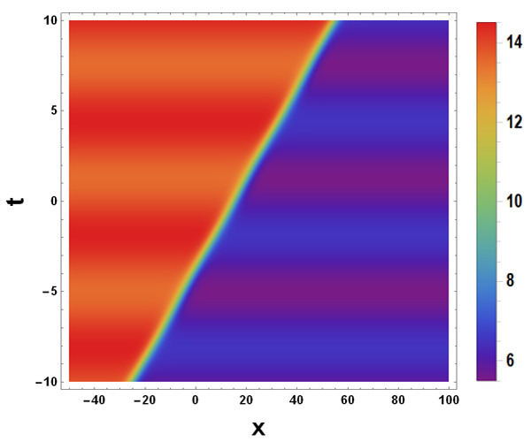
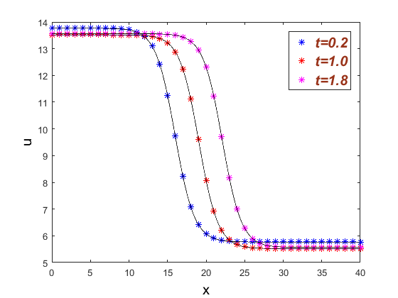
Fig. 3: (Color online) (a) Density plot of the theoretical solution (27); (b) Computational results and the theoretical solution of Example 3 at $t=0.2,1.0,1.8$. The meanings of discrete points and solid lines are the same as Fig. 1.

Example 4. Finally, we give the simulation for the theoretical solution with both the variable external-force and dispersive terms whose expression is presented by

$$u(x,t)=10-\frac{1}{2}\cos(5+t)+4\tanh\big{[}6+1.6t+\frac{4}{15}t^{3}-0.4x+6\cos(5+t)+3t\sin(5+t)\big{]}.$$ (28)

Fig. 4(a) shows that these two variable coefficients change both the amplitude and velocity ($\Delta x_{1}<\Delta x_{2}$) [21], and the definition of $\Delta x$ is the same as Example 2. As shown in Fig. 4(b), this situation combines two characteristics in Example 2 and 3. The GRE and relaxation time ($\tau$) of computational results are provided in Tab. 6.

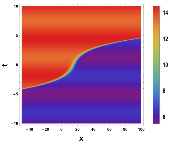
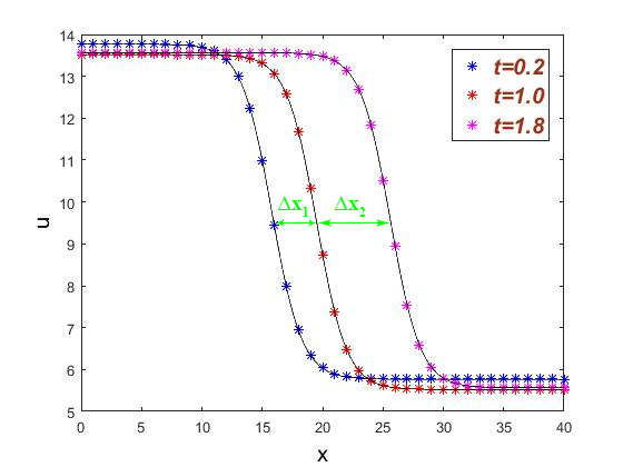
Fig. 4: (Color online) (a) Density plot of the theoretical solution (28). (b) Computational results and theoretical solutions of Example 4 at $t=0.2,1.0,1.8$. The meanings of discrete points and solid lines are the same as Fig. 1.

Tab. 6: The GRE and relaxation time ($\tau$) for computational results of Example 4

$t$	$t$=0.2	$t$=1.0	$t$=1.8
GRE	9.7555e-04	2.6925e-04	5.3918e-04
$\tau$	2.5324	3.4604	5.6684

4 Conclusions

In summary, the lattice Boltzmann model has been constructed for Eq. (1) by choosing the equilibrium distribution and compensatory functions. Eq. (1) has been recovered correctly through the Chapman-Enskog expansion. Four numerical examples have been studied when we take some appropriate parameters and they agree well with the theoretical results. Through our work, the dynamic characteristics affected by the dispersive and external-force coefficients, such as the velocity and amplitude, have been simulated effectively. Based on the error analysis, it has been found that the LBM could be applied to the variable-coefficient NLEEs with the external-force term.

References

- [1] R. Benzi, S. Succi, M. Vergassola, The lattice Boltzmann equation: theory and applications, Phys. Rep. 222 (1992) 145.
- [2] Y. H. Qian, D. D’Humières, P. Lallemand, Lattice BGK Models for Navier-Stokes Equation, Europhys. Lett. 17 (1992) 479.
- [3] R. S. Hirsh, Higher order accurate difference solutions of fluid mechanics problems by a compact differencing technique, J. Comput. Phys. 19 (1975) 90.
- [4] A. Dogan, A Galerkin finite element approach to Burgers’ equation, Appl. Math. Comput. 157 (2004) 331.
- [5] M. A. Helal, A Chebyshev spectral method for solving Korteweg-de Vries equation with hydrodynamical application, Chaos Soliton. Fract. 12 (2001) 943.
- [6] T. Geyikli, D. Kaya, An application for a modified KdV equation by the decomposition method and finite element method, Appl. Math. Comput. 169 (2005) 971.
- [7] S. Kutluay, A. R. Bahadir, A. Özdeş, A small time solutions for the Korteweg-de Vries equation, Appl. Math. Comput. 107 (2000) 203.
- [8] A. A. Soliman, A numerical simulation and explicit solutions of KdV-Burgers’ and Lax’s seventh-order KdV equations, Chaos Soliton. Fract. 29 (2006) 294.
- [9] D. Kaya, M. Aassila, An application for a generalized KdV equation by the decomposition method, Phys. Lett. A 299 (2002) 201.
- [10] C. Cercignani, Theory and application of the Boltzmann equation, Scottish Academic Press (1975).
- [11] Z. Shen, G. Yuan, L. Shen, Lattice Boltzmann method for Burgers equation, Chin. J. Comput. Phys. 17 (2000) 166.
- [12] C. Y. Zhang, H. L. Tan, M. R. Liu, L. J. Kong, Electromagnetism, Optics, Acoustics, Heat Transfer, Classical Mechanics and Fluid Mechanics-A Lattice Boltzmann Model and Simulation of KdV-Burgers Equation, Commun. Theor. Phys. 42 (2004) 281.
- [13] H. B. Li, P. H. Huang, M. R. Liu, L. J. Kong, Simulation of the MKdV equation with lattice Boltzmann method, Acta. Phys. Sini. 50 (2001) 837.
- [14] B. C. Shi, Z. L. Guo, Lattice Boltzmann model for nonlinear convection-diffusion equations, Phys. Rev. E 79 (2009) 016701.
- [15] T. Xu, C. Y. Zhang, J. Li, X. H. Meng, H. W. Zhu, B. Tian, Symbolic computation on generalized Hopf-Cole transformation for a forced Burgers model with variable coefficients from fluid dynamics, Wave Motion 44 (2007) 262.
- [16] L. Y. Cai, X. Wang, L. Wang, M. Li, Y. Liu, Y. Y. Shi, Nonautonomous multi-peak solitons and modulation instability for a variable-coefficient nonlinear Schrödinger equation with higher-order effects, Nonlinear Dyn. 90 (2017) 2221.
- [17] L. Wang, C. Liu, X. Wu, X. Wang, W. R. Sun, Dynamics of superregular breathers in the quintic nonlinear Schrödinger equation, Nonlinear Dyn. 94 (2018) 977.
- [18] F. P. Chen, W. Q. Chen, L. Wang, Z. J. Ye, Nonautonomous characteristics of lump solutions for a-dimensional Korteweg-de Vries equation with variable coefficients, Appl. Math. Lett. 96 (2019) 33.
- [19] L. Wang, X. Wu, H. Y. Zhang, Superregular breathers and state transitions in a resonant erbium-doped fiber system with higher-order effects, Phys. Lett. A 382 (2018) 2650.
- [20] L. Q. Kong, L. Wang, D. S. Wang, C. Q. Dai, X. Y. Wen, L. Xu, Evolution of incipient discontinuity for the defocusing complex modified KdV equation, Nonlinear Dyn. (2019) https://doi.org/10.1007/s11071-019-05222-z.
- [21] Y. T. Gao, X. G. Xu, B. Tian, Variable-coefficient forced Burgers system in nonlinear fluid mechanics and its possibly observable effects, Int. J. Mod. Phys. C 14 (2003) 1207.
- [22] H. Bateman, Some recent researches on the motion of fluids, Monthly Weather Rev. 43 (1915) 163.
- [23] J. Y. Zhang, G. W. Yan, A lattice Boltzmann model for the Burgers-Fisher equation, Chaos 20 (2010) 023129.
- [24] Z. H. Chai, B. C. Shi, L. Zheng, A unified lattice Boltzmann model for some nonlinear partial differential equations, Chaos Soliton. Fract. 36 (2008) 874.
- [25] H. L. Lai, C. F. Ma, A new lattice Boltzmann model for solving the coupled viscous Burgers’ equation, Phys. A 395 (2014) 445.