Castell: Scalable Joint Probability Estimation of Multi-dimensional Data Randomized with Local Differential Privacy

Abstract

Performing randomized response (RR) over multi-dimensional data is subject to the curse of dimensionality. As the number of attributes increases, the exponential growth in the number of attribute-value combinations greatly impacts the computational cost and the accuracy of the RR estimates. In this paper, we propose a new multi-dimensional RR scheme that randomizes all attributes independently, and then aggregates these randomization matrices into a single aggregated matrix. The multi-dimensional joint probability distributions are then estimated. The inverse matrix of the aggregated randomization matrix can be computed efficiently at a lightweight computation cost (i.e., linear with respect to dimensionality) and with manageable storage requirements. To overcome the limitation of accuracy, we propose two extensions to the baseline protocol, called hybrid and truncated schemes. Finally, we have conducted experiments using synthetic and major open-source datasets for various numbers of attributes, domain sizes, and numbers of respondents. The results using UCI Adult dataset give average distances between the estimated and the real (2 through 6-way) joint probability are $0.0099$ for truncated and $0.0155$ for hybrid schemes, whereas they are $0.03$ and $0.04$ for LoPub [4]), which is the state-of-the-art multi-dimensional LDP scheme.

I Introduction

With today’s widespread application of Internet of things (IoT) devices, our daily activities are continuously being scanned and monitored. This generates a huge amount of personal data, most of which contain values of for many personal attributes. These high-dimensional big data are useful for improving human life. For example, Shen et al. [2] proposed a method for aggregating high-dimensional data to improve the response to the demand for smart grids. Saint-Maurice et al. [1] found that a greater number of steps per day was associated with a significantly lower risk of all-cause mortality in US adults. However, the downside of such an accumulation of personal big data is that the data are very often highly privacy sensitive.

Local anonymization has been recognized as a good approach to privacy-preserving data collection since at least 1965, when randomized response (RR) was first proposed [13]. Under RR, the respondents individually anonymize their responses locally before the responses are sent to the data controller, who can thereafter accurately estimate the frequencies of the true responses from the collected RRs. Much more recently, local differential privacy (LDP) has added a differential privacy (DP) guarantee to RRs. For example, Erlingsson et al. at Google [16] proposed an LDP algorithm called the randomized aggregatable privacy-preserving ordinal response (RAPPOR), which is used by Google Chrome to collect user data in a privacy-guaranteed manner.

Unfortunately, neither the RR nor LDP algorithms can estimate the joint probability distribution of high-dimensional data because of the curse of dimensionality, which entails several issues:

• Exponential domain growth. The number of values (categories) of the Cartesian product of multiple domains grows exponentially. The analysis of the aggregated randomization matrix entails a high computational and communication costs.

• Loss of dependency. A simple way to circumvent the previous problem with the Cartesian product is to independently randomize each attribute in the response. However, doing so means losing any non-negligible dependencies among the attributes. Independently randomized values can be distributed almost uniformly and strongly associated pairs of data may be hidden over the aggregated domains.

• Domain sparsity. Domain sparsity is an additional undesirable consequence of the exponential growth of attribute combinations. Here, the combination of values increases exponentially, while the number of respondents remains constant. The number of respondents answering any specific combination therefore becomes very small. As the number of attributes increases, the distribution of the RR becomes sparse, which implies a loss of accuracy when estimating the frequencies of the original responses.

There have been many studies on high-dimensional data with DP or LDP guarantee including [36], [39], [35], [31], [37], [40], [32], and [38]. Most of these studies aim to inject DP noise and focus on the optimality of subsets of attributes to minimize estimation error. But, the dimensionality issues were not fully examined and estimation accuracy loss with dimensionality was not evaluated. Some recent works [4], [5], and [6] use RR for high-dimensional data in an LDP guarantees. Ren et al. [4] studied an LDP scheme called LoPub, estimating multi-dimensional joint probability distributions. Wang et al. [5] proposed an improvement scheme, called LoCop, which leveraged a multivariate Gaussian copula to estimate cross-attribute dependencies. Jiang et al. [6] introduced DP-FED-WAE, which combined a generative Wasserstein autoencoder (WAE) [7] with federated learning. However, the estimation accuracies were low and the dimensionality issue remained.

To address the dimensionality issues, Domingo-Ferrer and Soria-Comas [3] considered two extreme RR schemes, called RR-Joint and RR-Independent. RR-joint performs RR on the full domain, with respondents perturbing their data according to a predefined probability over the full domain and the server estimating a joint probability via the inverse probability matrix. The estimate is accurate but does not scale well in terms of dimensionality. Obtaining the inverse of the exponentially grown matrix is infeasible because of the complexity of the computation and communication costs. Conversely, RR-Independent performs a separate RR for each attribute and then estimates the marginal probabilities, whose product gives the estimated joint probability. This is scalable with dimension size in the sense that the computation cost is linear with respect to dimensionality, and the estimation accuracy is independent of dimensionality. However, its overall estimation accuracy is low, particularly when multiple attributes happen to be correlated strongly. To summarize, Table I shows the pros and cons of the two RR schemes.

TABLE I: The pros and cons of various RR schemes

	accuracy		efficiency
RR schemes	low dim.	high dim.	comp.	comm.
RR-Joint [3]	$\surd$	$\times$	$\times$	$\times$
RR-Independent [3]	$\times$	$\surd$	$\surd$	$\surd$
RR-Ind-Joint (§III-C)	$\surd$	$\times$	$\surd$	$\surd$
hybrid(§III-D)	$\surd$	$\surd$	$\surd$	$\surd$
truncated(§III-E)	$\surd$	$\surd$	$\surd$	$\surd$

To overcome the drawbacks of these two RR schemes, this paper proposes a new multi-dimensional RR scheme RR-Ind-Joint, whereby respondents randomize (in RR) all attributes independently, the server then aggregates these individual randomization matrices into a single aggregated matrix, and estimates jointly multi-dimensional joint probability distributions. As shown in Table I, the baseline RR-Ind-Joint runs efficiently at a lightweight computational cost for high-dimensional data and estimates the joint probability as accurately as RR-Joint.

However, because of the domain sparsity, the estimation loss increases exponentially with dimensionality. To address this limitation on accuracy, we propose two extensions to the baseline protocol, called hybrid (in Section III-D) and truncated (in Section III-E) schemes. The former combines the baseline scheme with RR-Independent to cover a broad range of dimensions and the latter truncates the joint probability of each of the $w$ attributes at an upper limit estimated by the joint probability of the lower ($w-1$)-dimensional data. Both extensions are efficient ways of improving the estimation accuracy and compensating for the estimation loss at high dimension, as shown in Table I.

Our schemes have the following advantages:

1. There exists a unique nonsingular accumulated randomization matrix for any attribute-independent randomized multi-dimension data. We show a simple way to construct the accumulated randomization matrix using the Kronecker product and a necessary condition for having an inverse matrix (Theorem 1).

2. Our joint probability estimation is accurate. All randomizations added independently are aggregated exactly and are removed completely by producing the inverse matrix. Our experiments with the Adult dataset [21] showed that the average variant distances between the estimated and the real (2-way through 6-way) joint probabilities are $0.0099$ for the truncated scheme and $0.0155$ for the hybrid scheme. These are $0.03$ and $0.04$, respectively, of that of LoPub[4], state-of-the-art multi-dimensional LDP scheme. The errors were also smaller than those for other schemes, including LoCop [5] and WAE [6].

3. The inverse of the aggregated randomization matrix is scalable. For the inverse matrix computation, we present an efficient algorithm, called castell, that requires ${\cal O}(wd^{2.807})$ computational cost (linear with respect to dimensionality) and $d^{w}$ memory for the matrix (the same size as for the $w$-way contingency table), where $w$ is the dimensionality of the data and $d$ is the domain size per attribute. Our experiments demonstrated the rapidity of the algorithm (0.007 seconds for the 6-way joint probability using the Adult dataset). The processing time increased $2\times 10^{-5}$ per dimension.

4. The estimation accuracy is guaranteed. We derive an the upper bound of estimation error for both RR-Ind-Joint and RR-Independent (see Theorem 1 and 5, respectively). This error estimation analysis enables the design of an optimal hybrid RR scheme that can switch between two estimation schemes to select the one best suited to the given set of parameter values for dimensionality, privacy budget, and number of respondents.

5. Privacy is guaranteed. We prove that the attribute-independent randomization of multi-dimensional data satisfies the LDP (see Theorem 3).

Our contributions to this work are as follows:

• We propose a new LDP scheme RR-Ind-Joint for multi-dimensional data and an algorithm that estimates the joint probability distribution from the observed frequencies of the randomized data. RR-Ind-Joint comprises an attribute-independent randomization (RR-Ind) and an inverse matrix computation algorithm castell that executes with low computational and communication costs .

• We calculate an upper bound for the estimation error of RR-Ind-Joint and RR-Independent in terms of dimensionality, the domain size, the privacy budget, and the number of respondents. Having established a formula for the estimation error, we can adopt a hybrid scheme involving RR-Ind-Joint and RR-Independent that contains an optimal estimation algorithm for any dimension.

• We conducted experiments to evaluate the performance of the proposed schemes using both synthetic and open-source datasets. Our results show that the proposed scheme can deal with a wide range of datasets and can estimate the joint probabilities as the estimated accuracy.

The rest of the paper is organized as follows. In Section II, we present some fundamental definitions and review some existing work related to multi-dimensional anonymization. Section III outlines our scheme and describes an algorithm for estimation. We also discuss privacy and the primary factors causing estimation errors. Section IV presents our experimental results using synthetic and open-source data, which verify that our model’s estimation errors are as claimed analytically. In Section VII, we conclude our study based on the proven theorems and the experimental results.

II Fundamental Definitions

II-A Randomized Response

An RR is a local anonymization mechanism whereby each data subject/respondent masks their own data/responses before forwarding them to a data controller. Each response item is randomly replaced by a new item with probabilities determined by a randomization matrix.

Definition 1

Let $X$ be a set of $d$ elements, labeled $1,\ldots,d$ without loss of generality. A $d\times d$ matrix of probabilities

$$P=\left(\begin{array}[]{rrr}p_{11}&\cdots&p_{1d}\\ \vdots&\ddots&\vdots\\ p_{d1}&\cdots&p_{dd}\end{array}\right),$$

is a randomization matrix of $X$ if and only if $p_{i1}+\cdots+p_{id}=1$ for $i=1,\ldots,d$ and $p_{uv}$ is the conditional probability of a randomized element being $v$, given that the true element is $u$, (i.e., $p_{uv}=Pr(Y=v|X=u)$ for all $u,v\in\{1,\ldots,d\}).$

An RR is a randomized mechanism whereby input $X$ of $d$ possible values $a_{1},\ldots,a_{d}$ is randomized to the response $Y$ according to $P$. By $Y=\textsf{RR}_{P}(X)$, we denote the algorithm defined in Algorithm 1. The goal of RR is to estimate the frequency of $a$ in $X$.

More specifically, if we let $\pi_{1},\ldots,\pi_{d}$ be the proportions of respondents whose true values fall in each of the $d$ values in $X$ and let $\lambda_{a}$ be the empirical probabilities of the observed values, we can write $(\lambda_{1},\ldots,\lambda_{d})^{T}=P^{T}(\pi_{1},\ldots,\pi_{d})^{T}.$ According to Warner [13], an unbiased estimator $\pi$ can be computed as $\hat{\pi}=(P^{T})^{-1}\hat{\lambda},$ where $\hat{\lambda}=(\hat{\lambda}_{1},\ldots,\hat{\lambda}_{d})^{T}$ is the vector of observed empirical probabilities for $Y$.

Algorithm 1 Randomization RR(X)

1:$x_{i}\leftarrow$ input of party $i$ for attribute $X$.

2:$P\leftarrow$ a randomization matrix for attribute $X$.

3:for all respondents $i=1,\ldots,n$ do

4:     $y_{i}\leftarrow\left\{\begin{array}[]{ll}x_{i}&\mbox{\rm w.p. $=p_{uu}$, $x_{i}$ is $u$-th element}\\ v&\mbox{\rm w.p. $=p_{uv}=q$}\end{array}\right.$

5:end for

6:return the randomized response $y_{1},\ldots,y_{n}$.

II-B Multi-Dimensional RRs

Here, we review in more detail the methods proposed by Domingo-Ferrer and Soria-Comas [3].

II-B1 RR-Joint

This is the natural way to apply RRs to multiple attributes. Given attributes $(A_{1},\ldots,A_{m})$, we consider the Cartesian product $A_{1}\times\ldots\times A_{m}$ as a single attribute and perform RR on it. The distribution of the true data is estimated as

$$\hat{\Pi}^{(X_{1},\ldots,X_{m})}_{\sf RR-Joint}=(P^{T})^{-1}\hat{\lambda}^{X_{1},\ldots,X_{m}}.$$ (1)

However, RR-Joint is severely affected by the curse of dimensionality, because the number of value combinations of $A_{1}\times\ldots\times A_{m}$ grows exponentially with the number $m$ of attributes. In computational terms, we must deal with matrices and vectors whose size is exponential in $m$, which is intractable except for small values of $m$. However, even if we had enough computational power, we face a more fundamental limitation, whereby Domingo-Ferrer and Soria-Comas [3] show that, for a fixed number of respondents, the error of the estimated frequencies also grows exponentially with $m$.

II-B2 RR-Independent

This is a basic approach in which RR is applied separately to each attribute, and the joint distribution is estimated by assuming that the attributes are independent of each other. Each party applies RR independently for each of the $m$ attributes $X^{1},\ldots,X^{m}$ in a dataset as $Y=(Y^{1},\ldots,Y^{m})$, where $Y^{j}=\textsf{RR}_{P^{j}}(X^{j})$. After estimating the marginal probabilities for the $j$-th attribute as $\hat{\pi}^{j}={({P^{j}}^{T})}^{-1}\hat{\lambda}^{j},$ the joint probability distribution for $X^{1},\ldots,X^{m}$ is estimated by the product of the marginal distributions as

$$\Pi^{(X_{1},\ldots,X_{m})}_{\sf RR-Ind}(a_{1},\ldots,a_{m})=\hat{\pi}^{1}(a_{1})\cdots\hat{\pi}^{m}(a_{m}).$$ (2)

Algorithm 2 shows the steps for this method. The issue with RR-Independent is that it only yields an accurate estimate when the independence assumption among attributes is (approximately) true.

Algorithm 2 Estimation RR-Independent$(Y)$

1:$\hat{\lambda}^{j}\leftarrow$ observed empirical probability for attribute $A^{j}$.

2:for all $j=1,\ldots,m$ do

3:     $\hat{\pi}^{j}\leftarrow((P^{j})^{T})^{-1}\hat{\lambda}^{j}$

4:end for

5:$\hat{\Pi}_{\sf RR-ind}^{(1,\ldots,m)}\leftarrow\hat{\pi}^{1}(x^{1})\dots\hat{\pi}^{m}(x^{m})$ for $A^{1}\times\cdots\times A^{m}$.

6:return $\hat{\Pi}_{\sf RR-ind}^{(1,\ldots,m)}$

II-B3 RR-Clusters

To overcome the issues with RR-Joint and RR-Independent, [3] proposed RR-Clusters. This method splits attributes into clusters according to their mutual dependence. That is, attributes within a cluster are highly dependent, whereas the dependence among attributes in different clusters is low. The method then proceeds by performing RR-Joint within each of the clusters, and assumes independence across clusters to estimate the joint distribution.

As a measure of independence, [3] used Cramer’s V statistics [8], which gives a value between 0 and 1, with 0 indicating complete independence between two attributes. Cramer’s $V_{ij}$ is defined as

$$V_{ij}=\sqrt{\frac{\chi^{2}_{ij}/n}{\min(d_{i}-1,d_{j}-1)}},$$

where $d_{i}$ is the number of values in attribute $A^{i}$ and $\chi^{2}_{ij}$ is the chi-squared independence statistic defined as

$$\chi^{2}_{ij}=\sum^{d_{i}}_{a=1}\sum^{d_{j}}_{b=1}\frac{(o^{ij}_{ab}-e^{ij}_{ab})^{2}}{e^{ij}_{ab}},$$

for which $o^{ij}_{ab}$ and $e^{ij}_{ab}$ are the observed and the expected frequencies of the combination $a$ and $b$, respectively.

III Proposed Method

III-A Problem Statement

Our goal is to perturb multi-dimensional data in order to obtain an LDP privacy guarantee, while being able to use the perturbed data to estimate the joint probability distributions for the true data.

Consider that $n$ respondents, each with a record of $m$ attributes (their respective true answers). Each attribute has a domain $\Omega_{i}$ of possible values. The full domain for the $m$ attributes is $\Omega=\Omega_{1}\times\cdots\times\Omega_{m}$. Each respondent uses RR to perturb their private answer $x_{i}^{1},\ldots,x_{i}^{m}$ into $y_{i}^{1},\ldots,y_{i}^{m}$ and submits the latter to a central server. Given this perturbed data $Y^{1},\ldots,Y^{m}$, where $Y^{i}=(y^{i}_{1},\ldots,y^{i}_{n})$, and a randomization mechanism (dependent on privacy budget $\epsilon$ of LDP), the central server aims to estimate the $w$-way joint probability distribution $\hat{\Pi}^{S}$ of a subset $S$ of $w\leq m$ attributes without having access to the respondents’ true data $X^{1},\ldots,X^{m}$.

We wish to obtain a solution with the following properties.

1. Accuracy. The estimated probability should be close to the true one. Namely, $\hat{\Pi}^{S}\approx\Pi^{S}$ for any $S$.

2. Scalability. The scheme scales dimension $w$ from computational and communicational (storage) perspectives. Since the full domain size $|\Omega|$ grows exponentially to $w$, we should manage to the domain expansion.

3. Generality. The scheme can be applied to a general multi-domain data without requiring any limitation.

III-B Idea

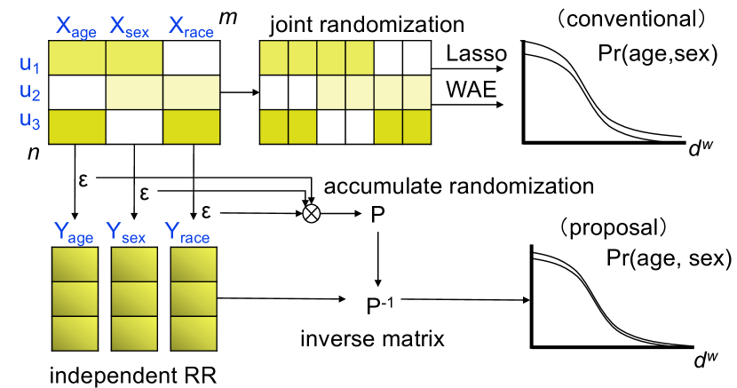
Figure 1: Overview of the proposed scheme

We illustrate the overview of our proposed scheme in Fig. 1, where $n=3$ respondents have $(m=3)$-dimensional records comprising values for three attributes, Age, Sex and Race. Some conventional studies randomize the matrix jointly and $w$-way joint probabilities are estimated via the Lasso regulation [4], or the WAE [6]. In contrast, our approach randomizes each attribute independently, according to the privacy budget $\epsilon$. The inverse of the aggregated randomization matrix allows us to revise the randomized processes added to the original high-dimensional data and estimate the $w$-way joint probability distribution.

To estimate the joint probability, we must overcome the following three difficulties. (1) The independently randomized attributes lose their dependencies. (2) The aggregated matrix grows exponentially with the dimensionality of the data. With $d$ elements per attribute, the aggregation of $w$ matrices leads to $d^{2w}$ dimensionality. It is therefore hard to compute the inverse matrix due to the computation and the communication complexities. (3) Because of the domain sparsity, the estimation loss increases as the dimensionality increases.

First, we construct the aggregated randomization matrix using the Kronecker product and the $w$ randomized matrixes. The aggregated randomization matrix recovers the hidden associations among attributes. We also give a necessary condition for the aggregated matrix to be nonsingular.

Second, we divide the problem of inverting the aggregated matrix into $w$ smaller subproblems using the properties of the Kronecker product. This reduces the computational complexity from ${\cal O}(d^{w})$ to ${\cal O}(dw)$, which is why it is called a reduced method). However, it still requires substantial storage for both the ${d^{w}}^{2}$ matrix and the inverse matrix before to be performed the product to the ($d^{w}$)-dimensional vector of the empirical probabilities. We therefore attempt to limit the storage overhead by performing $w$ inverse matrix products iteratively. Our proposed castell algorithm updates the multi-dimensional empirical probabilities incrementally by producing each inverse matrix, which requires a storage size of $d^{w}$ in total.

Finally, with regard to the domain sparsity issue, we propose the hybrid and truncated schemes. In the hybrid scheme, we combine the baseline scheme with RR-Independent to cover a broad range of dimensionalities. We calculate the upper bounds for the estimation error in both schemes (Theorem 5 for RR-Independent, and Theorem 6 for RR-Ind-Joint), which suggest thresholds for the features of high-dimensional data (the dimensionality, the number of respondents, and a privacy budget) that enable adoption of the most appropriate scheme. The truncated scheme truncates the joint probability of $w$ attributes at the upper limits estimated by the joint probability for the lower ($w-1$)-dimensional data.

III-C RR-Ind-Joint

III-C1 Randomization

The randomization process is the same as for RR-Independent. That is, suppose that $m$ attributes are independently randomized to give $m$ randomization matrices $P^{1},\ldots,P^{m}$, respectively. After the $n$ respondents perform the randomization processes to their respective answers $X=(X^{1}\ldots,X^{m})$ independently, giving $Y^{j}={\sf RR}_{P^{j}}(X^{j})$ for $j=1,\ldots,m$, a central server observes the perturbed records $Y=(Y^{1},\ldots,Y^{m})$. Here, $X$ and $Y$ are $m$-dimensional data for $n$ records over the full domain $\Omega$ defined by the Cartesian products of $m$ domains as $\Omega=\Omega_{1}\times\cdots\times\Omega_{m}$, where each domain size is $d_{i}=|\Omega_{i}|$ for $i=1,\ldots,m$.

When multiple attributes are randomized independently, can we find a joint randomization matrix that yields the same randomization and allows us to estimate the joint distribution? To answer this question, we leverage the independence of the attribute randomization. Specifically, two events $(a_{1}\rightarrow a_{2})$ and $(b_{1}\rightarrow b_{2})$ for attribute $A$ and $B$ are independent if and only if

$$Pr(a_{1}\rightarrow a_{2}\land b_{1}\rightarrow b_{2})=Pr(a_{1}\rightarrow a_{2})Pr(b_{1}\rightarrow b_{2}).$$

This makes the aggregation of multiple randomizations simple and practical. We now present the following theorem for obtaining the aggregated randomization matrix.

Theorem 1

Let $P^{i}$ and $P^{j}$ be nonsingular $(d_{i}^{2})$ and $(d_{j}^{2})$ randomization matrices for attributes $A^{i}$ and $A^{j}$, respectively. The matrix $P^{i}\otimes P^{j}$ is a non-singular $(d^{i}d^{j})^{2}$ randomization matrix for $(A^{i},A^{j})$.

By recursively applying Theorem 1 to every pair of attributes, it is straightforward to generalize it.

Corollary 1

Let $P^{i_{1}},\ldots,P^{i_{w}}$ be non-singular randomization matrices for $w$ attributes $A^{i_{1}},\ldots,A^{i_{w}}$. A matrix defined by $P^{i_{1}}\otimes\cdots\otimes P^{i_{w}}$ is a non-singular randomization matrix for $|\Omega^{i_{1}}|\times\cdots\times|\Omega^{i_{2}}|$ where $|\Omega^{i}|$ is a domain of attribute $A^{i}$.

A differential private randomization matrix with $p=\frac{e^{\epsilon}}{e^{\epsilon}+d-1}$, $q=\frac{1}{e^{\epsilon}+d-1}$ becomes singular only when $\epsilon=0$ and $p=1/d$. Because it is not hard to avoid the trivial case of $\epsilon=0$, we can confirm that there exists a non-singular accumulated randomization matrix for any given set of (non-singular) randomization matrices.

III-C2 Estimation

We now consider the estimation of the $w$-way joint probability distribution of set of attributes $S=\{A^{i_{1}},\ldots,A^{i_{w}}\}\subset\{A^{1},\ldots,A^{m}\}$ from the independently RRs $Y^{1},\ldots,Y^{m}$. Let $w$ be the size of subset $S$, i.e., $|S|=w\leq m$.

Given an aggregated randomization matrix $P^{i_{1}}\otimes P^{i_{w}}$, the $w$-way joint probability is given as

$$\hat{\Pi}^{S}=((P^{i_{1}}\otimes P^{i_{w}})^{T})^{-1}\lambda^{S},$$

where $\lambda$ is a $(d_{i_{1}}\cdot d_{i_{w}})$-dimensional vector for the empirical distribution of $Y^{i_{1}},\ldots,Y^{i_{w}}$.

III-C3 Inverse Matrix

The dominant cost in estimating the joint probability is for the matrix inversion. If Strassen’s algorithm [20], known as the best performing algorithm, is used, the inversion cost is ${\cal O}(|\Omega|^{2.807})$. We therefore must be able reduce the cost of matrix inversion for both computation and storage reasons.

Let us consider the inverses of aggregated matrix of $(d_{A}^{2})$ and $(d_{B}^{2})$ matrices $P_{A}$ and $P_{B}$, respectively. From the fundamental property of the Kronecker product that $(A\otimes B)^{-1}=A^{-1}\otimes B^{-1}$, we can compute the inverse matrix as follows,

$$\hat{\Pi}^{AB} = \left(P_{A}\otimes P_{B}\right)^{-1}\lambda^{AB}$$ (3)

$$= \left({P_{A}}^{-1}\otimes{P_{B}}^{-1}\right)\lambda^{AB}$$ (4)

where $\lambda^{AB}$ is a $(d_{A}\times d_{B})$-dimensional vector. (For simplicity, we omit the initial transpose of $P$ hereafter.) We call Eqs. (3), and (4) as naïve, and reduced, respectively. The reduced method divides the computational cost of the matrix inversion into those for lower-dimensional $d_{A}^{2}$ and $d_{B}^{2}$. However, it still requires the storage of the aggregated matrix, which is $(d_{A}\times d_{B})^{2}$ one. The aggregated matrix becomes too large to store realistically when $|\Omega|=d_{1}\times d_{w}>5000$.

Note that we are proposing the castell method that solves the inverse matrix while incurring only lightweight computation costs manageable storage requirements. Recall Eq. (4), which can be written as

$$= (P_{A}^{-1}\otimes P_{B}^{-1})\lambda^{AB}$$ (11)

$$= \left(\begin{array}[]{cc}a_{11}P_{B}^{-1}&a_{12}P_{B}^{-1}\\ a_{22}P_{B}^{-1}&a_{22}P_{B}^{-1}\end{array}\right)\left(\begin{array}[]{c}\lambda_{a_{1}b_{1}}\\ \lambda_{a_{1}b_{2}}\\ \lambda_{a_{2}b_{1}}\\ \lambda_{a_{2}b_{2}}\\ \end{array}\right)$$

$$= \left(\begin{array}[]{c}a_{11}P_{B}^{-1}\lambda_{a_{1}}+a_{12}P_{B}^{-1}\lambda_{a_{2}}\\ a_{21}P_{B}^{-1}\lambda_{a_{1}}+a_{22}P_{B}^{-1}\lambda_{a_{2}}\\ \end{array}\right)$$ (14)

$$= \left(\begin{array}[]{cc}a_{11}&a_{21}\\ a_{21}&a_{22}\\ \end{array}\right)\left(\begin{array}[]{c}P_{B}^{-1}\lambda_{a_{1}}\\ P_{B}^{-1}\lambda_{a_{2}}\\ \end{array}\right)$$ (19)

$$= P_{A}^{-1}P_{B}^{-1}\lambda^{AB},$$ (20)

where $(a_{ij})$ is an element of $P_{A}^{-1}$ and $\lambda_{a_{i}}$ of Eq. (14) is $d_{B}$-dimension vector $(\lambda_{a_{i}b_{1}}\,\lambda_{a_{i}b_{d_{B}}})^{T}$ for $i=1,\ldots,d_{B}$. Note that we assume $d_{A}=d_{B}=2$ here for simplicity. Eq. (20) is $(d_{A}\times d_{B})$-dimension vector $\hat{\Pi}^{AB}=\left(\begin{array}[]{c}\Pi^{AB}_{a_{1}}\\ \Pi^{AB}_{a_{2}}\end{array}\right)$. If we rearrange the vector as $d_{A}\times d_{B}$ matrix, Eq. (20) can be written simply as $(\Pi^{AB}_{a_{1}}\,\Pi^{AB}_{a_{2}})=P_{A}^{-1}\left(P_{B}^{-1}{\Lambda^{AB}}^{T}\right)^{T},$ where $\lambda^{AB}$ in Eq. (4) is replaced by $\Lambda^{AB}$, which is a $(d_{A}\times d_{B})$ matrix obtained by rearrangement of the elements of the $\lambda^{AB}$ empirical distribution over $(Y_{A},Y_{B})$. This is the basic idea in the castell method for matrix inversion. The computation for the castell inverse is as lightweight as that for the reduced method because it only requires the inversion of each $d_{i}^{2}$ matrix. The matrix size does not increase as it does for multi-dimensional data, and the storage size stays constant, irrespective of the number of dimensions being processed. It requires storage only for the empirical distribution $\Lambda^{AB}(=\lambda^{AB})$, which is proportional to $|\Omega|=d_{1}\times\cdots\times d_{w}$. Therefore, the castell inversion is efficient in terms of both computational and communicational costs.

To make the difference between the reduced and castell algorithms clear, we illustrate the two estimation steps in Fig. 2. Given three randomization matrices $P_{1}$, $P_{2}$ and $P_{3}$ having $d_{1}^{2}$, $d_{2}^{2}$ and $d_{3}^{2}$ dimensions, respectively, the 3-way joint probabilities $\Pi^{123}$ are estimated. Note that the estimated joint probabilities $\Pi^{123}$ in the vector for the reduced method are identical to those for the ($d_{1}\times d_{2}\times d_{3}$)-dimensional data $\Pi^{123}$ (i.e., the two estimations are mathematically equivalent).

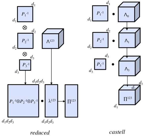
Figure 2: Flows in the joint probability estimation from three randomization matrices $P_{1},P_{2}$, and $P_{3}$ for the reduced and castell algorithms

To extend the basic idea of castell inversion to $w$-dimensional data, we introduce a new transposition for multi-dimensional data.

Definition 2

Let $A$ be $d_{1}\times d_{2}\times\cdots\times d_{w}$ multi-dimensional data $(a_{i_{1}\cdots i_{w}})$ for $1\leq i_{j}\leq d_{j}$. Then, $i$-th transposition of $A$ is a $d_{i}\times(d_{1}\cdots d_{i-1}d_{i+1}\cdots d_{w})$ matrix denoted by $A^{T_{i}}$ such that

$$A^{T_{i}} = \left(\begin{array}[]{ccc}a_{\cdots 1\cdots 1}&\cdots&a_{\cdots 1\cdots d_{w}}\\ \vdots&\ddots&\vdots\\ a_{\cdots d_{i}\cdots 1}&\cdots&a_{\cdots{d_{i}}\cdots d_{w}}\\ \end{array}\right).$$ (24)

The inverse of $i$-th transposition, denoted by $A^{T_{i}^{-1}}$, is a $d_{1}\times\cdots\times d_{w}$ multi-dimensional data such that $(A^{T_{i}})^{T_{i}^{-1}}=A$.

Note that $A^{T_{i}}$ is a matrix (2-dimensional data) and $A^{T_{i}^{-1}}$ is a multi-dimensional data. The rows of the matrix in Eq. (24) are ordered according to the $i$-th attribute and the columns can be arranged arbitrarily. We now introduce a simple method for arranging the columns via a permutation $\sigma$ of the sequence of dimension identities $\langle 1,2,\ldots,w\rangle$. For example, consider the 3-dimensional data comprising race, sex, and income, with domain sizes $d_{1}=5$, $d_{2}=2$, and $d_{3}=2$, respectively. Let $\Lambda$ be the empirical distribution for $S=\{A_{race},A_{sex},A_{income}\}$ (comprising $5\times 2\times 2=20$ elements) as

$$\left(\left(\begin{array}[]{cc}1&6\\ 2&7\\ 3&8\\ 4&9\\ 5&10\\ \end{array}\right),\left(\begin{array}[]{cc}11&16\\ 12&17\\ 13&18\\ 14&19\\ 15&20\\ \end{array}\right)\right).$$

By letting $\sigma$ be a permutation of the sequence $\langle 1,2,3\rangle$, where $\sigma(1)=3,\sigma(2)=1$, and $\sigma(3)=2$ for the $(i=2)$-th transposition, we have $d_{2}\times d_{3}\cdot d_{1}=2\times 10$ matrix

$$\Lambda^{T_{2}}=\left(\begin{array}[]{cccccccccc}1&11&2&12&3&13&4&14&5&15\\ 6&16&7&17&8&18&9&19&10&20\\ \end{array}\right)$$

and the inverse transposition defined by $\sigma^{-1}(1)=d-i+2=2$, $\sigma^{-1}(2)=3$, and $\sigma^{-1}(3)=1$ gives a $d_{1}\times d_{2}\times d_{3}$ multi-dimensional data.

A general castell inversion of matrix is defined as follows. Let $P_{1},\ldots,P_{w}$ be randomization matrices. Given an empirical distribution $\Lambda^{S}$ of $d_{1}\times\cdots\times d_{s}$ dimensionality, the $w$-way joint probability is estimated as

$$\hat{\Pi}^{S}={P_{1}}^{-1}\left(\cdots\left(P_{w-1}^{-1}\left(P_{w}^{-1}{\Lambda^{S}}^{T_{w}}\right)^{T_{w}^{-1}T_{w-1}}\right)^{\cdots}\right)^{T_{1}}.$$

Note that the inverse of transposition $T_{i}^{-1}$ is inserted for every $i$-th product. This leaves the order of dimensions in the empirical distribution $\Lambda$ unchanged when cascading the $w$ products. That is, the estimate $\hat{\Pi}$ always remains a $(d_{1}\times d_{2}\times\cdots\times d_{w})$ dimensional data.

To implement this approach of computing the estimates incrementally, we present the Algorithm 3, which is a procedure for estimating the joint probabilities of the $w$ attributes from independently RRs $Y^{1}\ldots Y^{w}$.

Algorithm 3 Estimation RR-Ind-Joint, Castell

1:$P_{1},\ldots,P_{m}\leftarrow$ randomization matrices.

2:$Y^{i}\leftarrow{\sf RR}_{P_{i}}(X^{i})$ for $i=1,\ldots,m$.

3:$S\subset\{A^{1},\ldots,A^{m}\}$ such that $|S|=w$.

4:$\hat{\Lambda}^{S}\leftarrow$ $(d_{1}\times\cdots\times d_{w})$-dimension data of empirical distribution for attributes $(Y^{1},\ldots,Y^{m})$.

5:$\Lambda_{w}\leftarrow\hat{\Lambda}^{S}$.

6:for all $i=w,\ldots,1$ do

7:     $\Lambda_{i-1}\leftarrow(P_{i}^{-1}\Lambda_{i}^{T_{i}})^{T_{i}^{-1}}$

8:end for

9:return $\hat{\Pi}^{S}\leftarrow\Lambda_{0}$

We assume the use of Strassen’s algorithm [20] for the primitive matrix inversions and a domain size for the $w$ attributes of $d_{1}=\cdots=d_{w}=d$, for simplicity.

Theorem 2

Let $\Lambda$ be a $(d^{w})$-dimensional data representing the empirical distribution of $w$ attributes. Algorithm 3 runs in ${\cal O}(wd^{2.807})$ time and requires $d^{w}$ of storage.

Table II summarizes the computation and storage costs for three matrix inversion algorithms.

TABLE II: Costs for matrix inversion

method	inverse	computation cost	storage cost
1. naïve	$(P_{1}\otimes P_{2}\otimes P_{3})^{-1}$	${\cal O}(d^{w2.807})$	$d^{2w}$
2. reduced	$P_{1}^{-1}\otimes P_{2}^{-1}\otimes P_{3}^{-1}$	${\cal O}(wd^{2.807})$	$d^{2w}$
3. castell	$P_{1}^{-1}P_{2}^{-1}P_{3}^{-1}$	${\cal O}(wd^{2.807})$	$d^{w}$

III-D Hybrid Scheme

We now consider a hybrid scheme positioned between RR-Independent and RR-Ind-Joint. As we will show shortly in Sections III-G and III-H, RR-Ind-Joint is efficient when $w$ is small and $n$ is large, whereas estimation via RR-Independent is stable, simple, and less dependent on the dimensionality $w$. It is therefore useful to consider a hybrid of these two schemes for estimating probabilities in a more general environment.

The optimal algorithm will depend on the given data, for which several parameters are involved. Fortunately, our analysis shows that the estimation accuracy is monotonic (increasing/decreasing) with respect to the parameters; $n$ (a number of respondents) $\epsilon$ (a privacy budget), and $w$ (dimensionality) for both schemes. An optimal estimation algorithm can therefore be found by switching between RR-Independent and RR-Ind-Joint at predetermined threshold $n^{*}$, $\epsilon^{*}$, and $w^{*}$. Table III shows an example of the thresholds estimated for the Adult dataset ($n=32,561$ and $d=16$ (education)). (The detailed analysis is given in Appendix -C.)

TABLE III: Thresholds for selecting the optimal algorithm as either RR-Ind-Joint or RR-Independent

threshold	Adult dataset	scheme
$n>n^{*}$	121,000
$\epsilon>\epsilon^{*}$	0.473	RR-Ind-Joint
$w<w^{*}$	1.374
otherwise		RR-Independent

III-E Truncated Scheme

An estimation method that uses the inverse matrix could generate an invalid probability, such as a negative value, or a value greater than $1.0$. In addition to restricting these trivial invalid values, we develop a heuristic for regulating the estimated error growth, based on the relationship between the joint and the marginal probabilities as

$$Pr(A,B) = Pr(A|B)Pr(B)\leq Pr(B),$$

$$= Pr(B|A)Pr(A)\leq Pr(A),$$

$$\leq \min(Pr(A),Pr(B)).$$

We leverage this relationship to give the generalized inequality

$$0\leq Pr(S)\leq\min_{S^{\prime}\subset S,|S^{\prime}|=|S|+1}Pr(S^{\prime}).$$ (25)

This represents a limitation on the valid elements of the estimated probabilities. Using the limits estimated for $w-1$ dimensionality, we can truncate a too-high probability at the $w$ level, as shown in Algorithm 4.

Algorithm 4 Estimate improvement Truncated

1:$S=\{A^{1},\ldots,A^{w}\}$ a subset of set of $m$ attributes.

2:$\hat{\Lambda}^{S}\leftarrow$ $\Omega=(d_{1}\times\cdots\times d_{w})$-dimension data of empirical distribution for attributes $(Y^{1},\ldots,Y^{m})$.

3:$\hat{\Pi}^{S}\leftarrow$ Castell $(\hat{\Lambda}^{S})$

4:$\Pi_{0}\leftarrow\hat{\Pi}^{S}$ where all minus values are replaced with $0$.

5:for all $i=1,\ldots,w$ do

6:     $S_{i}\leftarrow S-\{A^{i}\}$

7:     $\Pi_{i}(a)\leftarrow$ $\min(\Pi_{i-1}(a),\mbox{{\em Castell}}(\Lambda^{S_{i}}(a)))$ for $a\in\Omega$.

8:end for

9:return $\Pi_{w}$

III-F Privacy

The privacy of the RR-ind-joint scheme is the same as that of RR-Ind. Consider a simple RR that gives a response $x$ with a probability of $p=\frac{e^{\epsilon}}{e^{\epsilon}+d-1}$ and gives a randomly chosen value in $\Omega_{A}$ as a response with a probability of $q=(1-p)/(d-1)=\frac{1}{e^{\epsilon}+d-1}$

The LDP holds for all independent RR attributes as follows.

Theorem 3

RR-Ind-Joint satisfies $(\epsilon,0)$-LDP for attribute $A$. With $m$ attributes $A^{1},\ldots,A^{m}$, RR-Ind-Joint satisfies $(m\epsilon,0)$-LDP.

Because LDP guarantees that it is unable to infer the true value from a randomized one, it does not provide DP [19]. LDP is related to attribute inference attack [27] and DP prevents membership inference attack [26]. According to Yeom et al. [25], attribute inference is at least as difficult as membership inference. Therefore, we think that a multi-dimensional data randomized to meet the LDP guarantee implies it will also meet the DP guarantee.

III-G Estimation Error (RR-Independent)

We evaluate the accuracy loss for the estimated joint probability in terms of the mean absolute error (MAE), the mean absolute error (MAE) and the average variation distance (AVD). MAE is defined as $MAE=1/{d^{2}}\sum_{x\in|A|\times|B|}|\Pi^{AB}(x)-\hat{\Pi}^{AB}(x)|.$ AVD was suggested by [4] and [6]. Let $C$ be a subset of attributes $\{X^{i_{1}},\ldots,X^{i_{w}}\}$. The AVD between the real joint probability distributions $\Pi^{C}$ and the estimated distributions $\hat{\Pi}^{C}$ is defined as

$$\mbox{\em AVD}=\frac{1}{|A|}\sum_{C\in A}\sup_{(c\in C}|\Pi^{c}-\hat{\Pi}^{c}|,$$

where $A$ is a power set of attributes such that $C$ has $w$ distinct attributes.

First, we show a bound for the MSE of RR-Independent.

Theorem 4

Let $A$ and $B$ be two attributes with Cramer’s V statistics $V$ and the same number of values in both domains, i.e., $d=|A|=|B|$. The MSE of RR-Ind is less than $V^{2}/d$.

Taking the squared root of both sides, we estimate that the MAE for RR-Independent is proportional to $V/\sqrt{d}$

Next, we consider an upper bound for the estimation error when $w$-way joint probability is estimated by RR-Independent. Assume that the marginal probability $\pi(a)$ for $a\in A^{i}$ is proportional to the domain size $|\Omega_{i}|=d_{i}$, for all $i\leq w$. The $w$-way joint probability is then

$$\Pi^{S}_{\sf RR-Ind}(a_{1},\ldots,a_{w})=\hat{\pi}^{1}(a_{1})\cdots\hat{\pi}(a_{w})=\frac{1}{d_{1}}\cdots\frac{1}{d_{w}}.$$

We can now identify a range of possible values for the joint probability, as follows.

Lemma 1

Let $\Pi$ be a real $w$-way joint probability of $w$ attributes with marginal probabilities $\pi^{1},\ldots,\pi^{w}$. Then, for any $a_{1},\ldots,a_{w}$ of $w$ attributes,

$$0\leq\Pi(a_{1},\ldots,a_{w})\leq\min(\pi^{1}(a_{1}),\ldots,\pi^{w}(a_{w}))$$

holds.

This means that the estimated probability must belong within the interval $[0,\min(\pi^{1},\ldots,\pi^{w})]$. We can derive an upper bound for the estimation error in RR-Independent as follows.

Theorem 5

Let $\hat{\pi}^{i}$ be the estimated marginal probability of the $i$-th attribute, which follows a uniform distribution of $1/d_{i}$, where $d_{i}$ is the size of the $i$-th domain for $i=1,\ldots,w$. A $w$-way joint probability of $w$ attributes is estimated by RR-Independent with an error less than

$$\max(d_{*}^{-w},1/d_{*}-d_{*}^{-w}),$$ (26)

error where $d_{*}=\max_{i\leq w}d_{i}$.

III-H Estimation Error (RR-Ind-Joint)

The MAE of RR-Ind-Joint does not depend on $V$ because it estimates the joint probability of attributes via inversion of the randomization matrix. RR-Ind-Joint has no estimation error provided all randomization matrices for the attributes are non-singular.

The estimation of RR-Ind-Joint suffers a rounding error in the empirical probability distribution $\lambda^{AB}(Y)$. The observed probability of $(a,b)$ for $Y$ is the fraction of respondents who send $(a,b)$ out of the $n$ respondents. The precision of empirical probability $\lambda^{AB}(Y)$ is therefore $1/n$. We consider a model of empirical probability having the form, $\hat{\lambda}=\lambda+\Delta\lambda,$ where $\lambda$ is the real joint probability of the randomization matrix and $\Delta\lambda$ is the rounding error. For example, suppose that we observe the empirical probability of a set of $n=10$ perturbed records as

$$\hat{\lambda}^{AB}=\left(\begin{array}[]{c}3/10\\ 3/10\\ 1/10\\ 3/10\end{array}\right)=\left(\begin{array}[]{c}0.2875\\ 0.2625\\ 0.1625\\ 0.2875\end{array}\right)+\left(\begin{array}[]{r}0.0125\\ 0.0375\\ -0.0625\\ 0.0125\end{array}\right),$$

where the empirical probabilities are the sums of the expected values, determined by a randomization mechanism ($P^{A}$, $P^{B}$ and $f^{X}$ (see Appendix -B)) and the rounding error $\Delta\lambda$.

We consider the rounding error as a uniform distribution over $[-1/n,1/n]$, for which $E[\Delta\lambda]=0$ and $E[|\Delta\lambda|]=1/2n$ holds. Note that the rounding errors are within the range $-1/10<-0.0625<0.0375<1/10.$ Using this model, the estimation of the joint probability is

$$\hat{\Pi}=P^{-1}\hat{\lambda}=P^{-1}(\lambda-\Delta\lambda)=\Pi-P^{-1}\Delta\lambda.$$

The last term in the above formula is the source of the estimation error. It is a linear combination of $d^{2}$ uniform distributions and can be approximated as a normal distribution whose mean increases with $1/n$.

Lemma 2

Let $P$ be a randomization matrix for a set of $d$ elements with $p_{ii}=p=e^{\epsilon}/(e^{\epsilon}+d-1)$ and $p_{ij}=1/(e^{\epsilon}+d-1)$ for $i\neq j\in\{1,\ldots,d\}$. An element of $P^{-1}$ is at most $1/p$.

Lemma 3

Let $X_{1}$ and $X_{2}$ be attributes of $n$ records with domains of size $d_{1}$ and $d_{2}$, respectively. An independently randomized matrix $P$ with $\epsilon$-DP has a rounding error such as

$$\max P^{-1}\Delta\lambda<\left(1+\frac{\max(d_{1},d_{2})-1}{e^{\epsilon}}\right)^{2}\frac{d_{1}d_{2}}{n}$$

Theorem 6 (upper bound of estimation error)

A $w$-way joint probability distribution of $n$ records with domain sizes $d_{1},\ldots,d_{w}$, respectively, is estimated from an independently randomized matrix with $\epsilon$-DP in RR-Ind-Joint with an error not exceeding

$$\left(1+\frac{d-1}{e^{\epsilon/w}}\right)^{w}\frac{d^{w}}{n},$$ (27)

where $d=\max(d_{1},\ldots,d_{w})$.

Note that the estimation error is asymptotically linearly related to the size of the full domain $|\Omega|=d_{1}\times\cdot\times d_{w}<d^{w}$.

IV Evaluation

IV-A Data

We evaluate the utility loss in RR processing and estimating using four major open-source datasets and a synthetic dataset (see Appendix -D).

Table IV shows the specifications for the open-source datasets that are required to evaluate the performance of the proposed schemes. We chose major open-source datasets that comprised multi-dimensional data records. Each dataset has $n$ records (rows) of $w$ attributes (columns). Each attribute has a domain $\Omega$ of possible values. The full domain for the $w$-dimensional data is denoted by the Cartesian product of all attributes $\Omega=\Omega_{1}\times\cdots\times\Omega_{w}$. We denote the size of the full domain by $|\Omega|$. Generally, $|\Omega|$ increases exponentially with data dimensionality $w$. For example, the US Census dataset has 68 categorical attributes with several domain sizes ranging from 2 (Sex, iKorean) to 18 (iYewarsch). The full domain is $1.7\times 10^{44}$. Depending on the dataset, we randomly choose 20 – 50 combinations of $w$ attributes to form $A$ and take the average of the estimation errors (distances) for the $w$-way joint distributions.

TABLE IV: Dataset specifications

dataset	description	# records $n$	# att. $w$	domain size $\Omega_{i}$
Adult	UCI census income data [21]	32,561	8	1814400
Census	US Census Data (1990) [22]	2,458,285	68	1.711505e+44
Credit	German Credit Data (2000) [23]	1,000	13	34,560,000
Nursery	Enrollment data in 1980’s Nursery school [24]	12,960	9	64,800

IV-B Results (Open-source Data)

Table V shows the MAE for two attribute values in the Adult dataset: namely, $n=32,561$ and privacy budget $\epsilon=1$.

TABLE V: Example MAE for the Adult dataset

	sex	income	sex	race	edu.	occupa.
$d$	2	2	2	5	16	15
$V$	0.216		0.118		0.187
RR-Ind	$1.88\times 10^{-3}$		$1.10\times 10^{-4}$		$2.15\times 10^{-5}$
RR-Ind-Joint	$7.07\times 10^{-10}$		$2.26\times 10^{-9}$		$6.28\times 10^{-7}$

Fig. 3 shows the AVD between the real and the estimated joint probability distributions with respect to dimensionality $w$. We estimate the $w$-way joint probability via LoPub [4] (Lasso regression with the 64 bits for Bloom filter and 5 hash functions) and via the proposed RR-Ind-Joint method.

The AVDs for RR-Ind-Joint are distributed around $4^{-4}$ to $1^{-2}$ for $w\leq 4$. There are quite small in comparison to LoPub. The accuracy is very high in comparison with any recent multi-dimensional LDP schemes such as LoCop [5] and Wasserstein autoencoder (WAE) [6] (According to Fig. 5 [6], the AVDs for LoCop are close to those for LoPub and the AVDs of WAE are almost half of those for LoPub and LoCop. The estimation results of WAE are in the range $0.05$ to $0.09$. )

Fig. 3 also shows the AVDs of the multi-dimensional RR schemes RR-Independent and RR-Joint [3]. Because of the exponential nature of computational and capacity costs, the estimating via RR-Joint with the dimensionality of more than 3 was not feasible. The AVDs for RR-Ind-Joint are much better than those for RR-Independent. Note that we have plotted the AVDs using a logarithmic scale. Table VI shows that the hybrid and truncated schemes outperform the conventional works and the AVDs for 6-way joint probabilities of hybrid and truncated schemes are $0.0155$ and $0.0099$, which is $0.03$ of that in LoPub with the same condition.

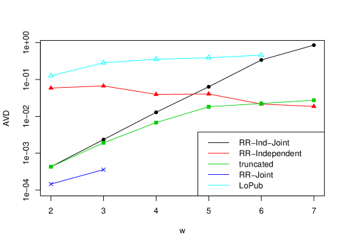
Figure 3: AVDs for several algorithms with respect to the dimensionality $w$

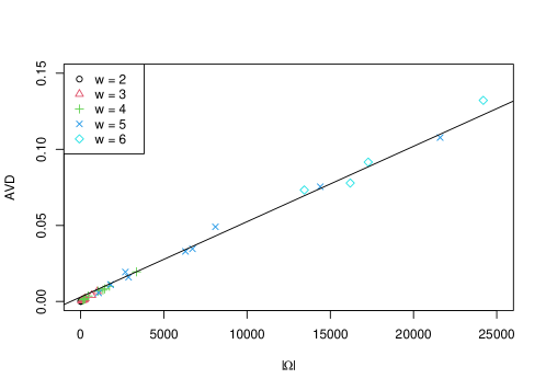
Figure 4: AVDs for RR-Ind-Joint with respect to the domain size $|\Omega|$

TABLE VI: AVDs of various schemes (the Adult dataset, $n=32,561,\epsilon=4,|\Omega|=16800$)

schemes $\backslash\,w$	2	3	4	5	6	mean
RR-Ind-Joint	0.0004	0.0023	0.0129	0.0635	0.3384	0.0835
RR-Independent	0.0588	0.0669	0.0395	0.0405	0.0215	0.0455
hybrid	0.0004	0.0023	0.0129	0.0405	0.0215	0.0155
truncated	0.0004	0.0019	0.0068	0.0182	0.0223	0.0099
RR-Joint [3]	0.0001	0.0004				0.0003
LoPub [4]	0.1262	0.2832	0.3560	0.3891	0.4576	0.3224

The AVD increases exponentially as the dimensionality $w$ increases and increases linearly with the full domain size $|\Omega|=|\Omega_{1}\times\cdots\times\Omega_{w}|$, where $\Omega_{i}$ is the domain of $i$-th attribute. The estimation error is related to the full domain size $|\Omega|$. Fig. 4 shows a scatter plot of AVD against the domain size $|\Omega|$. It shows that the domain size $|\Omega|$ varies with the dimensionality $w=2,\ldots,5$ and that the AVD is linear with respect to $|\Omega|$. In the figure, the maximum domain size $|\Omega|=16,800$ is given by the product of $|\Omega_{race}|=5$, $|\Omega_{education}|=16$, $|\Omega_{occupation}|=15$, $|\Omega_{marital-status}|=7$, and $|\Omega_{income50k}|=2$. Fitting the AVD to a linear function, we have a simple prediction

$$\hat{\mbox{\em AVD}}(|\Omega|)=2.944\cdot 10^{-3}+4.953\cdot 10^{-6}|\Omega|.$$ (28)

If we assume a maximum error as $\mbox{\em AVD}^{*}=0.5$, solving Eq. (28) gives the maximum domain size $|\Omega^{*}|=100,365$.

Fig. 5 shows the AVDs of $w$-way joint probability distributions estimated for RR-Ind-Joint. All datasets show similar behavior, in that the AVDs increase exponentially with $w$, as $d^{w}$. This is consistent with the upper bound given by Eq. (27). The standard deviation, shown as the 68% confidence interval of $\pm\sigma$, also grows with $w$ (excessively long intervals that have negative values are not shown).

In Fig. 5, the AVDs of estimated by RR-Independent are shown in red. The AVDs estimated by RR-Independent increase with $w$ ($-p^{w}$) when $w$ is small and turns to be decreasing ($\min(p_{i})$). Compared to the RR-Ind-Joint case, the estimated joint probabilities are distributed stably. We can therefore conclude that RR-Ind-Joint estimates joint probabilities more accurately than RR-Independent for small dimensionality $w$. However, if $w$ is sufficiently large, RR-Independent is more accurate than RR-Ind-Joint. There is always a crossover point $w^{*}$ within which RR-Ind-Joint estimates accurately for all datasets. For example, using the Adult dataset, we would prefer RR-Ind-Joint for estimating $w$-way joint probabilities if $w\leq 4$, with RR-Independent being preferred otherwise. The crossover points for the other datasets are $w^{*}=8,3$, and $4$ for US census, Credit and Nursery, respectively.

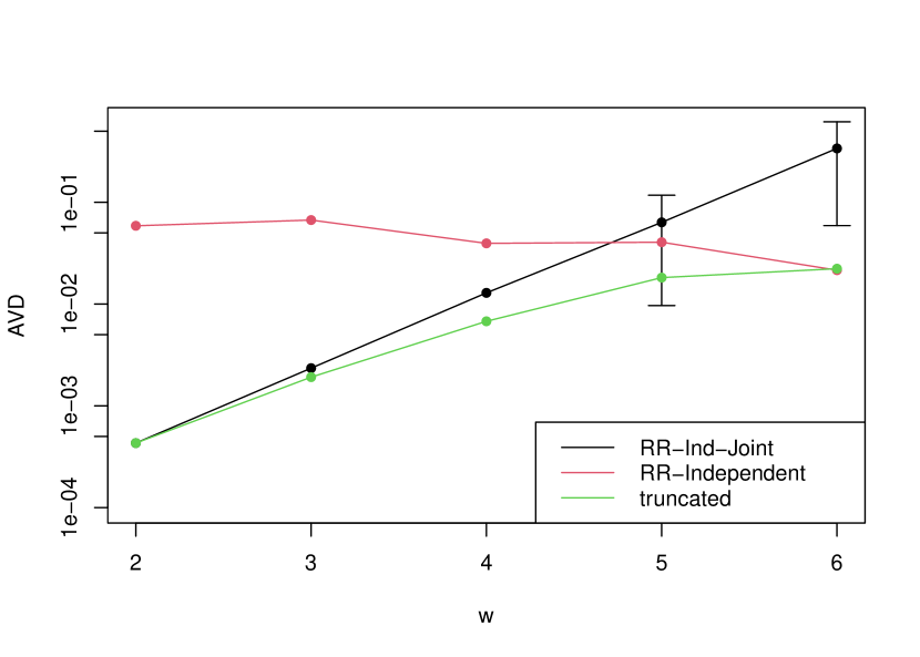
(a) Adult

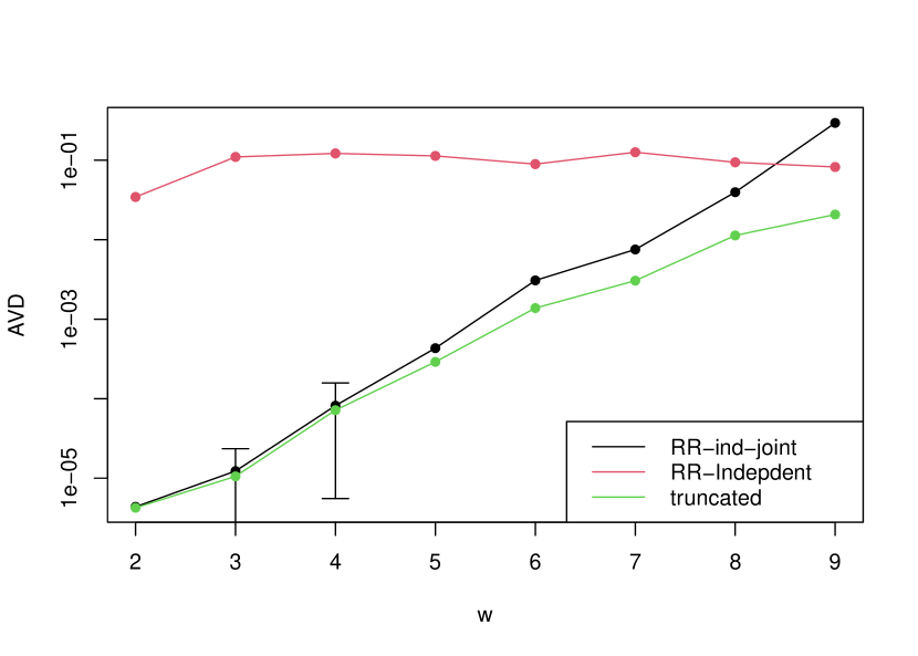
(b) US Census

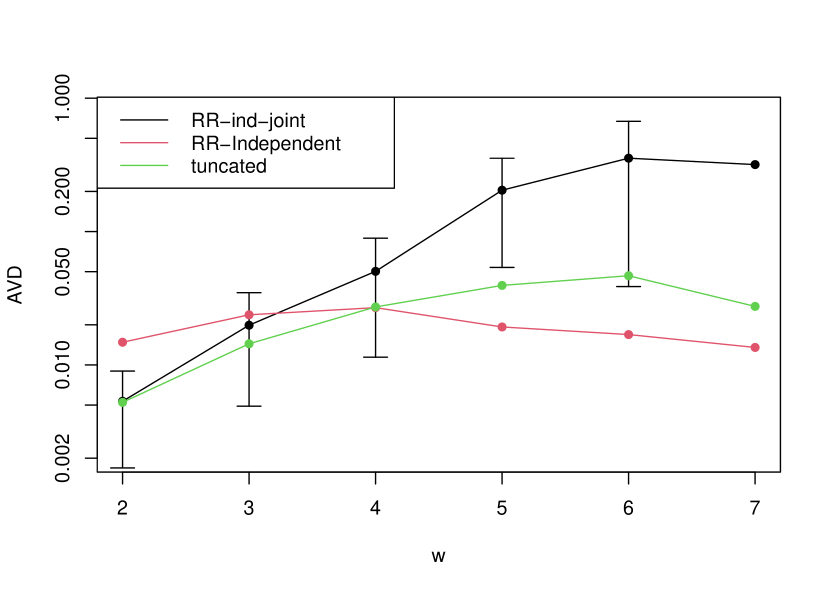
(c) Credit

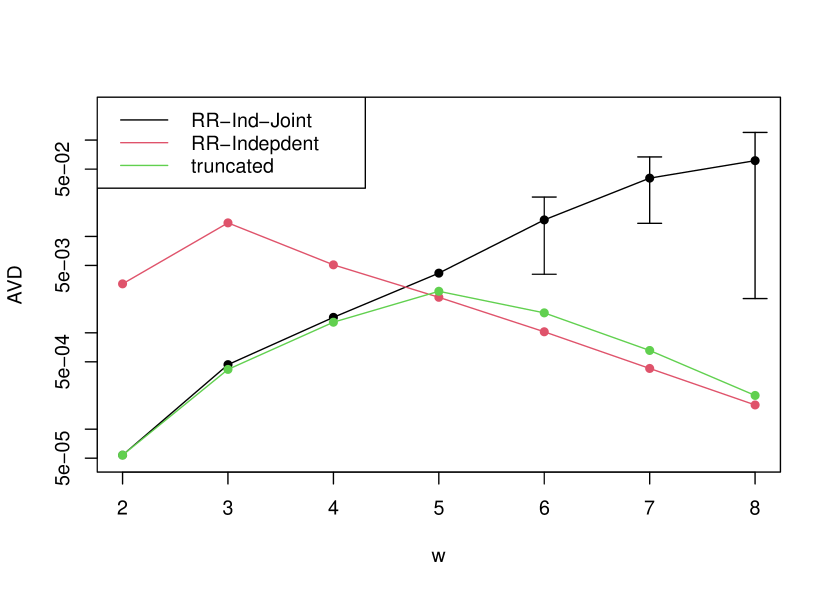
(d) Nursery

Figure 5: AVDs between real and estimated values for $w$-way joint probabilities with respect to dimensionality $w$

The upper bound for the AVD using RR-Ind-Joint in Eq. (27) indicates that the AVD and number of respondents $n$ are inversely proportional. Fig. 6 shows the distributions of AVDs with respect to the number of respondents (records) $n$. We see that RR-Ind-Joint estimates probabilities more accurately than RR-Independent when $n$ is large for all datasets. This result suggests that RR-Ind-Joint is the most appropriate when $n>500$, in most cases.

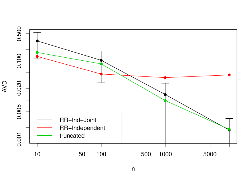
(a) Adult

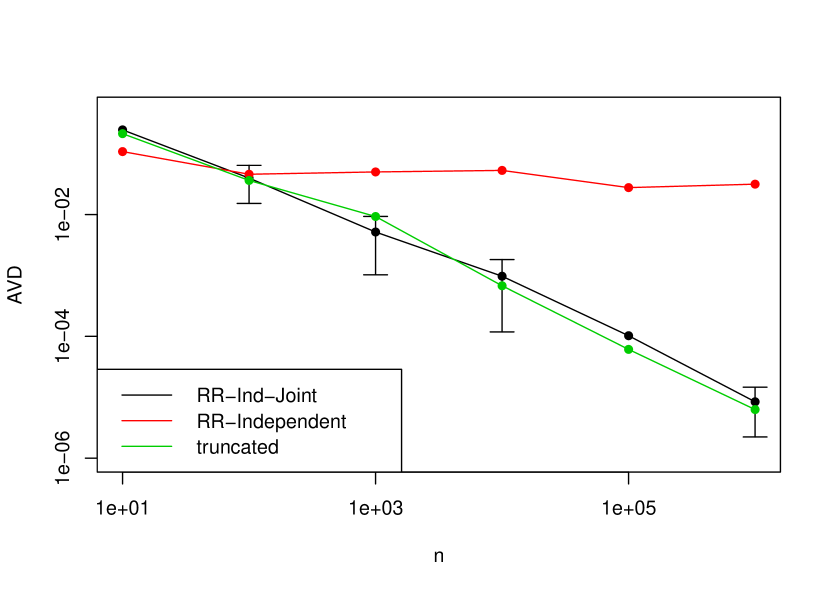
(b) US Census

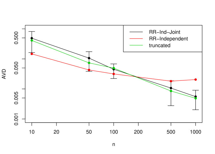
(c) Credit

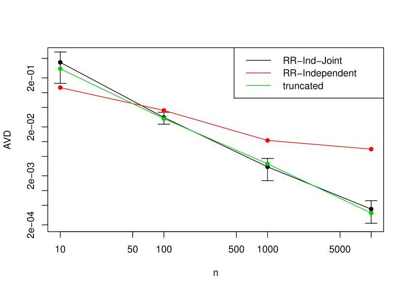
(d) Nursery

Figure 6: AVD between real and the estimated $(w=2)$ way joint probabilities with respect to the number of respondents $n$

Estimation error depends on privacy budget $\epsilon$. The AVDs of RR-Ind-Joint decrease as $\epsilon$ increases because Eq. (27) converges to $d^{w}/n$ when $\epsilon$ becomes large. In contrast, the estimation error for RR-Independent are independent of $\epsilon$ because the error incurred by the independence of attributes dominates in this case. Fig. 7 shows the AVDs of $2$-way joint probabilities using RR-Ind-Joint and RR-Independent. The datasets were perturbed with privacy budget $\epsilon$ ranging from $0.5$ to $8$. Note that the AVDs for RR-Ind-Joint decrease as the privacy budget $\epsilon$ increases, whereas the AVDs for RR-Independent are stable. Except for cases where $\epsilon=0.5$ for the Adult and Credit datasets, RR-Ind-Joint is indicated as the preferred option for estimation.

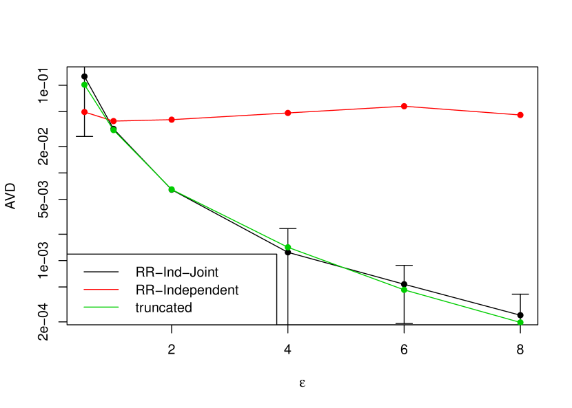
(a) Adult

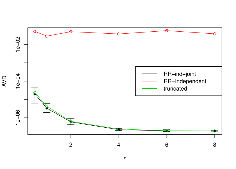
(b) US Census

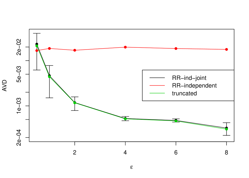
(c) Credit

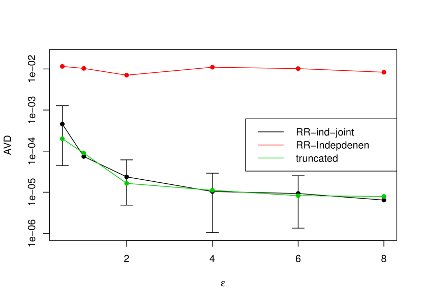
(d) Nursery

Figure 7: AVDs between real and the estimated $2$-way joint probabilities with regard to privacy budget $\epsilon$

IV-C Processing Time

RR-Ind-Joint is scalable with respect to the dimensionality $w$ of the joint probability estimation. In Algorithm 3, the inverses are computed for each of $w$ randomization matrices having $(d_{j},d_{j})$ dimensions for $j=1,\ldots w$ rather than inverting a $(d_{1}\times\cdots d_{w},d_{1}\times\cdots d_{w})$-dimension matrix, which would require both a large computational capability and a large amount of storage. We show the reduction of computation cost in Fig. 8, as the processing time for computing the inversion of a $(3^{w},3^{w})$ matrix with $p=0.5$ for $w=2,\ldots,6$ dimensionality. The measurements were repeated 100 times in R version 4.0.0, running on a 2.3-GHz Intel Core i9, with 32 GB DDR4. The figure shows that the processing time for $(P\otimes\cdots\otimes P)^{-1}$ computations (labeled as “naïve”) increases exponentially with $w$, whereas the processing time for $(P^{-1})\otimes\cdots\otimes(P^{-1})$ computations (labeled as “reduced”) increases more slowly. The computation time at $w=6$ is $0.007$ seconds. The castell inversion algorithm not only reduces the storage requirements for the matrix but also helps minimize the computation time.

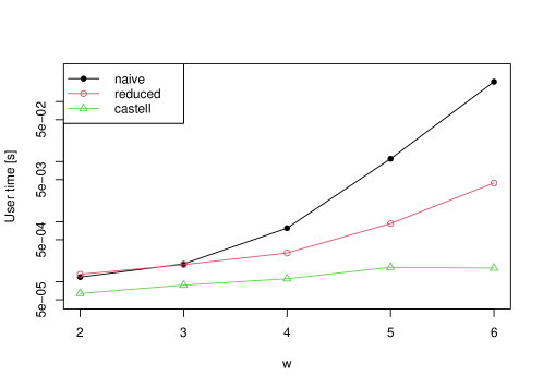
Figure 8: Comparison of processing time for estimations as a function of dimensionality $w$

V Discussion

V-A Limitations

Although our scheme scales up high-dimension data, it still requires storage for the $d^{w}$ multi-dimensional contingency table for empirical distribution. The cross-tabulation for counting the combination of all attributes is available for R (table) and python (Pandas crosstab method) and is out of scope of this work. But, it is used inside of Algorithm 3 (for empirical distribution) and may have the limitation.

The upper bounds of estimation loss (Theorem 1 and 5) assume that $d=d_{1}=\cdots=d_{m}$ (domain size) for simplicity. In practice, it does not hold generally and hence the bounds are loose when the variance of domain size is large ($d$ ranges from $2$ to $16$ and has median $6.5$ in Adult data). This insufficient accuracy would incur the error of thresholds in hybrid scheme. For example, Table. III provides the thresholds estimated by the upper bounds, suggesting RR-Ind-Joint algorithm as preferable for $w<w^{*}=1.374$. However, according to the experimental results in Fig. 5, RR-Ind-Joint outperforms for $w<5$. For an alternative estimation of thresholds, a sampling-based analysis should be considered.

In the evaluation in Section IV, we dropped numerical attributes such as Age, Capital-gain/loss, Hour-per-week, and Country (42 values). Although numerical attributes can be converted to categorical ones, it is not trivial to identify the optimal number of bins. An automated and adaptive algorithm for the optimal granularity for conversion to categorical attributes is one of the future works.

V-B Extensions

The accurate joint probability estimation could follow an accurate synthetic data. For example, several synthetic algorithms have been proposed in LoPub [4], LoCop [5] and WAE [6]. LoPub performs random sampling of clusters of attributes and assigns values according to the estimated conditional distributions. LoCop uses the inverse cumulative distribution function for the multivariate Gaussian copula. The WAE generates a random vector from Gaussian distribution at the latent layer and feeds them into the decoder of the autoencoder. We will explore the best synthetic algorithms and evaluate the accuracy for major machine learning algorithms as one of the future studies.

RR-Ind-Joint is very accurate for low dimensionality. Hence, privacy-preserving key-value data is one of its potential applications. With an appropriate conversion of numerical values to categorical date, we can apply RR to key-value data with LDP guarantee and estimate accurate the joint probability distribution that reveals the correlations between keys and values.

VI Related Works

VI-A Differential Private Data Publishing

DP [19] has been used for privacy protection in data publishing. LDP [11] was proposed to eliminate the assumption of trust in a central server and applied to many use cases including crowdsourcing participants [34], and heavy hitter detections [41], [42]. There were significant studies for useful building blocks and properties; a compositional theorem [18], an optimized local hashing (OLE) [29], a sampling-based approach [30], post-processing for improving utility [45] and on the optimal data-independent noise distribution [43].

For the works related to our goal, the attempts for multi-dimensional data publishing with DP or LDP are classified into some categories; the (Laplacian or Gaussian) Noise-based: [36], [39], [35], [31], [37], [40], [32], [38], the RR-based: [33], [28], [3],[5],[6], the Key-Value based (2-dimensional data) schemes: [14], [9], [27].

VI-B Multi-Dimensional LDP schemes

VI-B1 Nose-based schemes

The first attempt to add Laplace noise to high-dimensional data was done by Ding et al. [36]. They injected DP noise into an initial subset of cuboids and then compute the remaining cuboids from the initial subset. To improve accuracy of $w$-way marginal estimation, several studies have been done. PriView due to Qaraji et al. [39], [35] uses an entropy maximization. PrivBayes proposed by Zhang et al. [31] uses a Bayesian network to iteratively learn a set of low-dimensional conditional probabilities. Chen et al. [37] uses a junction tree algorithm to find the optimal mechanism based on sampling-based testing to explore pairwise dependencies of attributes. DPSense proposed by Day and Li [40] controls sensitivity with a threshold of counts and proves the optimization of the thresholds. CALM proposed by Zhang et al. [32] partitions the set of users into some groups and assigns them to one group, and then aggregates to obtain a noisy marginal table and performs reconstruction steps. DPPro studied by Xu et al. [38] uses a random projection to maximize utility and to preserve pairwise distances between attributes. They add Gaussian noise to intermediate vectors to maximize the utility and proves DP. Arcolezi et al. [46] proposed sampling techniques for saving privacy budget and shows the 9-way MSE of the Adult datasets. Cormode et al. [47] provided the utility guarantee and evaluated the estimate using open-source trajectory datasets.

Most of these studies aimed to satisfy DP rather than LDP and focused on the optimality of subsets of attributes to minimize estimation error. Hence, no sufficient evaluation of estimation accuracy with respect to $w$ were made. It is hard to compare our work for scalability.

VI-B2 RR-based schemes

RR [13] based multi-dimensional studies were inspired after RAPPOR [16] successfully encoded data as a Bloom Filter and then performs RR of each bit of filter. Soon after RAPPOR, Fanti et al. [33] proposed 2-dimensional joint probabilities using the Expectation Maximization (EM) algorithm. However, it incurs a considerable computational cost for higher dimension data. Wang et al. [28] theoretically derive a mathematical model of the mean squared error of RR and Laplace mechanism and show frequency estimation.

Recently, some advanced works [3], [4], [5], and [6] using RR for high-dimensional data were made. Domingo-Ferrer and Soria-Comas proposed some RR-based schemes toward the dimensionality issues. Their study, reviewed detailed in Section II-B, provides insights but has some drawbacks that motivate this work. Ren et al. [4] proposed an LDP scheme called LoPub, estimating multi-dimensional joint probability distributions. They perturb a multi-dimensional data encoded binary vectors using Bloom filter and combine a Lasso regression with an EM to estimate the joint probabilities accurately. They also show a method for synthetic data that preserves the utility of the original data in the sense that classification accuracies for some machine learning algorithms are preserved as the original. LoCop [5] improves LoPub by introducing multivariate Gaussian copula to estimate cross-attribute dependencies. To improve the accuracy of LoPub and LoCop, Jiang et al. [6] combines the Wasserstein Autoencoder (WAE) and the federated learning to propose DP-FED-WAE framework. With an LDP algorithm called SignDS for saving privacy budget, they reported that DP-FED-WAE outperforms LoPub and LoCop. They show the comparison of joint probability estimation accuracy in terms of $w$-way joint probabilities. We showed that RR-Ind-Joint outperforms the state-of-art schemes in Fig. 3 and Table VI.

VI-B3 Key-Value schemes

Key-value data has been used for several services and its privacy-preserving has a high demand. As for dimensionality, the dimension is fixed as $w=2$, but some studies deal with dependency between key and value similar to our study.

Nguyen et al. [14] proposed Harmony in which for any numerical data is encoded as binary data according to the value. Using Harmony as building block, Ye et al. [9] proposed an LDP protocol designed for key-value data. Their scheme perturbs the key jointly with the encoded value using a variation of RR. The associations between key and value are preserved from the randomized pairs with the privacy of input being guaranteed in a specified privacy budget. Note that PrivKV randomizes key and value jointly with probability depending on value. Fang et al. [27] study the local model poisoning attack to LDP schemes. Under assumption that attacker manipulates the value on the compromised device, they report some defense techniques have limited success in open data experiments.

VII Conclusion

In this paper, we have studied the randomization of a multi-dimensional data, where independent randomization of attributes would seem to address the curse of dimensionality. However, a naïve approach to independent randomization can suffer from three main drawbacks. First, the combination of domains grows exponentially. Second, the approach masks any association among attributes. Third, there can be too few records to cover the combined domain (the domain sparsity).

Our proposed multi-dimensional RR scheme RR-Ind-Joint randomizes all attributes independently, and estimates jointly the multi-dimensional joint probability distributions, while addressing these issues.

Using an accumulated arbitrary number of independent randomization matrices, we can estimate the joint probability with high accuracy. We have proposed a castell algorithm, which inverts its aggregated randomization matrix efficiently, and requires only lightweight computation costs (linear with respect to dimensionality $w$) and manageable storage costs ($d^{w}$, which is the same as for the cross-tabulation matrix). We develop upper bounds of the estimation errors for two primitive RR schemes (RR-Ind-Joint and RR-Independent) and propose a hybrid RR scheme that switches efficiently between them, depending on the values of the relevant parameters (dimensionality, the privacy budget, and the number of respondents). Our experimental results using open-source datasets show that the proposed scheme can deal with a wide range of datasets and can estimate joint probabilities to practical levels of accuracy.

We plan to tighten the upper bounds for the estimation errors. The estimated crossover points given in Table III are too large to serve as practical threshold values, such as were observed in Figs. 5, 6, and 7. In our current experiments, we ignore some continuous attributes that should be studied in the future.

Acknowledgment

-A Proofs

• First, we show that the matrix has a corresponding conditional probability. Let $u$ and $v$ be tuples of attributes $A^{i}$ and $A^{j}$ such that $u=(y^{i},y^{j})$ and $v=(x^{i},x^{j})$. From the premise of the randomization matrix for attributes $A^{i}$ and $A^{j}$, $p^{i}_{x^{i}y^{i}}=Pr[Y^{i}=y^{i}|X^{i}=x^{i}]$ and $p^{j}_{x^{j}y^{j}}=Pr[Y^{j}=y^{j}|X^{j}=x^{j}]$ hold. According to the definition of the Kronecker product, we obtain the $(d^{i}d^{j})\times(d^{i}d^{j})$ matrix as

  $$P^{i}\otimes P^{j}=\left(\begin{array}[]{ccc}p_{11}P^{j}&\cdots&p_{1d_{i}}P^{j}\\ \vdots&\ddots&\vdots\\ p_{d_{i}1}P^{j}&\cdots&p_{d_{i}d_{i}}P^{j}\end{array}\right),$$

  where element $p_{uv}$ is $p^{i}_{y^{i}x^{i}}\cdot p^{j}_{y^{j}x^{j}}$, which is equal to the joint probability of $u$ and $v$ because the two randomizations are independent. Second, we show it satisfies the conditions for probability. If $p_{11}+\cdots p_{1d_{i}}=1$ and $p_{11}+\cdots p_{1d_{j}}=1$, the sum of the Kronecker product $p_{11}p_{11}+\cdots+p_{1d_{i}}p_{1d_{j}}=p_{11}(p_{11}+\cdots+p_{1d_{j}})+\cdots+p_{1d_{i}}(p_{11}+\cdots+p_{1d_{j}})=p_{11}(1)+\cdots+p_{1d_{i}}(1)=1$ holds. Finally, we show that the matrix can be inverted. Because of the property of Kronecker products, $P^{i}\otimes P^{j}$ is non-singular if and only if $P^{i}$ and $P^{j}$ are non-singular. Hence, we have the theorem. $\Box$

• A permutation $\sigma_{i}$ takes $w$ time. The time for the transposition and its inversion are negligible because these can be predetermined from the data structure. An inversion of a $d^{2}$ matrix takes ${\cal O}(d^{2.807})$ time. Therefore, repeating these costs $w$ times, the total processing time is ${\cal O}(wd^{2.807})$ and the storage requirement of $d^{w}$ is constant. $\Box$

• For any $x,x^{\prime}\in|A|$ such that $x\neq x^{\prime}$, and any $y\in|A|$

  $$\frac{Pr[RR(x)=y]}{Pr[RR(x^{\prime})=y]}=\frac{p}{q}=e^{\epsilon}$$

  Because the $m$ attributes are perturbed independently, the sequential decomposition theorem [10] states that RR-Ind-Joint satisfies $(m\epsilon,0)$-LDP. $\Box$

• The definition of V statistics is $V=\sqrt{\chi^{2}/n(d-1)}$. Squaring and dividing both sides by $d$, we have

  $$V^{2}/d = \frac{\chi^{2}/n}{d(d-1)}\leq\frac{1}{nd^{2}}\sum^{d^{2}}_{i=1}\frac{(o_{i}-e_{i})^{2}}{e_{i}}$$

  $$= \frac{1}{d^{2}}\sum_{a\in|A|,b\in|B|}\frac{(o_{(a,b)}/n-\hat{\lambda}_{a}\hat{\lambda}_{b})^{2}}{\hat{\lambda}_{a}\hat{\lambda}_{b}}$$

  $$\leq \frac{1}{d^{2}}\sum_{a\in|A|,b\in|B|}(\Pi^{AB}(a,b)-\hat{\lambda}_{a}\hat{\lambda}_{b})^{2}$$

  $$= MSE(\Pi^{AB}).$$

  Note that the expected value $e_{i}$ is the mean of the binomial distribution of $p=\Pi^{AB}_{RRInd}$ with $n$ trials, i.e., $np=n\hat{\lambda}^{A}(a)\hat{\lambda}^{B}(b)$. The final inequality holds when $\hat{\lambda}_{a}\hat{\lambda}_{b}\leq 1.0$. $\Box$

• Suppose there exists an $i$-th attribute and value $a_{i}$ for which $\pi^{i}(a_{i})<\Pi(a_{1},\ldots,a_{w})$. This immediately contradicts the marginal probability given as $\sum_{a\in\Pi^{i}}\Pi(a_{1},\ldots,a,\ldots,a_{w})>\pi^{i}(a_{i})$. $\Pi(a_{1},\ldots,a_{w})$ must therefore be less than the minimum for $\pi^{j}$. $\Box$

• Given sufficient records and an accurate randomization matrix, a marginal distribution can be estimated without error. We consider this as $\hat{\pi}=\pi$. With the premise that $\pi^{i}\sim 1/d_{i}$ and Lemma 1 holds, the estimated probability is

  $$0 \leq \Pi^{S}_{\sf RR-Ind}(a_{1},\ldots,a_{w})=\frac{1}{d_{1}\cdots d_{w}}\leq\frac{1}{(\max d_{i})^{w}}$$

  $$\leq \min(\pi^{1}(a_{1}),\ldots,\pi^{w}(a_{w}))=\frac{1}{\max{d_{i}}}.$$

  Therefore, the longer interval either $[0,1/\max(d_{i})^{w}]$ or $[1/(\max d_{i})^{w},1/\max{d_{i}}]$ is an upper bound on the estimation error. $\Box$

• The adjugate matrix of $P$ shows that the largest elements of the inverse are along the diagonal and are less than $1/p$ for any $d\geq 2$. $\Box$

• The inverse of the product is given as $P^{-1}=P_{1}^{-1}\otimes P_{2}^{-1}$, whose largest elements are along the diagonal and are at most $1/p_{1}p_{2}$ from Lemma 2. $\Delta\lambda$ is a $(d_{1}\times d_{2})$-dimensional vector of uniform random values within $[-1/n,1/n]$. The rounding error is the inner product of $P^{-1}$ and $\Delta\lambda$ such that

  $$\max P^{-1}\cdot\Delta\lambda\leq(1/p_{1}p_{2}\cdots 1/p_{1}p_{2})\cdot\left(\begin{array}[]{c}1/n\\ \vdots\\ 1/n\end{array}\right)=\frac{d_{1}d_{2}}{p_{1}p_{2}n}$$

  $\Box$

• With $\epsilon^{\prime}=\epsilon/w$, $w$ attributes are randomized independently. From Lemma 3 and $\epsilon^{\prime}$, we have

  $$\max P^{-1}\Delta\lambda<\frac{d_{1}\cdots d_{w}}{p_{1}\cdots p_{w}n}<\frac{d^{w}}{p^{w}n}=\left(\frac{e^{\epsilon/w}+d-1}{d^{\epsilon/w}}\right)^{w}\frac{d^{w}}{n}$$

  where $d=\max(d_{1},\ldots,d_{w})$ and $p=\min(p_{1},\ldots,p_{w})$. $\Box$

-B Example

Consider a dataset $X$ on $n=10$ parties with two attributes $A$ and $B$, where domain $\Omega_{A}=\{a_{1},a_{2}\}$ and $\Omega_{B}=\{b_{1},b_{2}\}$. The empirical (true) joint probability distribution of $X$ is

$$\Pi_{AB}(a_{1},b_{1}) = 4/10,$$

$$\Pi_{AB}(a_{2},b_{1}) = 2/10,$$

$$\Pi_{AB}(a_{1},b_{2}) = 0,$$

$$\Pi_{AB}(a_{2},b_{2}) = 4/10.$$

This yields marginal distributions $\pi_{A}=(0.4,0.6)$ and $\pi_{B}=(0.6,0.4)$. We express the frequencies of $X$ as a $2\times 2$ matrix $f^{X}=\left(\begin{array}[]{cc}4&0\\ 2&4\end{array}\right),$ which indicates frequencies of $(a_{1},b_{1}),(a_{2},b_{1}),(a_{1},b_{2}),(a_{2},b_{2})$ for $X$, respectively.

With $\epsilon=\log(3)$ and $p_{A}=p_{B}=3/4$, we have randomization matrices for $A$ and $B$ as

$$P^{A}=\left(\begin{array}[]{cc}p_{A}&q_{A}\\ q_{A}&p_{A}\\ \end{array}\right)=\left(\begin{array}[]{cc}3/4&1/4\\ 1/4&3/4\\ \end{array}\right)=P^{B},$$

where $p=\frac{e^{\log 3}}{e^{\log 3}+d-1}=3/4$ and $q=1-p$. The respondents randomize their two responses $x_{i}^{A}$, and $x_{i}^{B}$ independently. Suppose that the randomized $Y^{A}=\textsf{RR}_{P^{A}}(X^{A})$ and $Y^{B}=\textsf{RR}_{P^{B}}(X^{B})$ are observed as $f^{Y}=\left(\begin{array}[]{cc}3&1\\ 3&3\end{array}\right),$ for which the empirical probabilities of $Y$ are $\lambda^{A}=(0.4,0.6)$ and $\lambda^{B}=(0.6,0.4)$. Note that the $V$ statistics for $A$ and $B$ gives $V_{AB}(Y)=0.25$, which is reduced from $V_{AB}(X)=0.66$ for the original dataset. Here, the correlation between $A$ and $B$ has been partially lost by the independent randomizations.

RR-Independent estimates the joint probabilities as the product of the estimated marginal distributions $\hat{\pi}^{A}={P^{A}}^{-1}\lambda^{A}=(0.3,0.7)$ and $\hat{\pi}^{B}={P^{B}}^{-1}\lambda^{B}=(0.7,0.3)$, giving

$$\hat{\Pi}^{AB}_{\sf RR\mathchar 45\relax Ind}=\left(\begin{array}[]{cc}0.21&0.09\\ 0.49&0.21\end{array}\right),$$

which estimates $\Pi^{AB}$ with MSE$=0.041$ and AVD = $0.29$. The value for $V$ statistics is nearly 0.

RR-Ind-Joint treats the two independent randomization matrices as a single accumulated matrix $P^{A}\otimes P^{B}$

$$=\left(\begin{array}[]{cccc}p_{a}p_{b}&p_{a}q_{b}&q_{a}p_{b}&q_{a}q_{b}\\ p_{a}q_{b}&p_{a}p_{b}&q_{a}q_{b}&q_{a}p_{b}\\ q_{a}p_{b}&q_{a}q_{b}&p_{a}p_{b}&p_{a}q_{b}\\ q_{a}q_{b}&q_{a}p_{b}&p_{a}q_{b}&p_{a}p_{b}\end{array}\right)=\frac{1}{16}\left(\begin{array}[]{cccc}9&3&3&1\\ 3&9&1&3\\ 3&1&9&3\\ 1&3&3&9\end{array}\right).$$

Given the observed the empirical distributions for $Y$, we estimate the joint probabilities as

$$\hat{\Pi}^{AB}_{\sf RR\mathchar 45\relax Ind\mathchar 45\relax Joint} = (P^{A}\otimes P^{B})^{-1}\Lambda^{AB}$$

$$= {P^{A}}^{-1}\left({P^{B}}^{-1}{\Lambda^{AB}}^{T}\right)^{T}$$

$$= {P^{A}}^{-1}\left(\left(\begin{array}[]{cc}1.5&-0.5\\ -0.5&1.5\end{array}\right)\left(\begin{array}[]{cc}0.3&0.1\\ 0.3&0.3\end{array}\right)^{T}\right)^{T}$$

$$= \left(\begin{array}[]{cc}1.5&-0.5\\ -0.5&1.5\end{array}\right)\left(\begin{array}[]{cc}0.4&0.3\\ 0.&0.3\end{array}\right)^{T}$$

$$= \left(\begin{array}[]{cc}0.45&-0.15\\ 0.25&0.45\end{array}\right).$$

The estimation error is MSE $=0.0075$ and AVD $=0.15$.

Using the limit on valid probabilities estimated via the $(w-1)$-way joint (marginal) probabilities $\hat{\pi}^{A}=(0.3,0.7)$ and $\hat{\pi}^{B}=(0.6,0.4)$, we obtain the revised probability for the truncated algorithm

$$\hat{\Pi}^{AB}_{truncated} = \left(\begin{array}[]{cc}\min(0.45,0.3,0.7)&\min(0,0.3,0.3)\\ \min(0.25,0.7,0.7)&\min(0.45,0.7,0.3)\\ \end{array}\right)$$

$$= \left(\begin{array}[]{cc}0.3&0\\ 0.25&0.3\\ \end{array}\right),$$

which improves accuracy as MSE $=0.15$ and AVD $=0.1$.

The privacy of the independent randomization is assured by $\epsilon=\ln(p/q)=\ln(3)$. With two attributes, the privacy budget is $2\epsilon=2\ln 3$ in total. The same privacy is assured by RR-Joint with $p^{\prime}=\frac{e^{2\epsilon}}{e^{2\epsilon}+d_{1}d_{2}-1}=9/12$, and $q^{\prime}=1/12$ and is expressed as

$$\frac{1}{12}\left(\begin{array}[]{cccc}9&1&1&1\\ 1&9&1&1\\ 1&1&9&1\\ 1&1&1&9\\ \end{array}\right)$$

for which $(2\ln 3,0)$-LDP holds.

-C Thresholds analysis for hybrid scheme

Experimental results in Fig. 5, 6 and 7 suggest that there are crossover points between two estimations.

By combining the upper bound of estimation error of RR-Ind-Joint in Eq. (27) with that of RR-Independent in Eq. (26), we identify the thresholds for number of respondents $n^{*}$ beyond which AVD_RR-Ind-Joint is less than AVD_RR-Ind as,

$$n^{*}\geq\left(1+\frac{d-1}{e^{\epsilon/w}}\right)^{w}\frac{d^{w}}{\max(d^{-w},1/d-d^{-w})},$$

where $d$ is the maximum domain size for $w$ attributes. It implies that RR-Ind-Joint shall be chosen when there are enough records $n$ according to the domain size $d=|\Omega|$ and dimension $w$. We see that (c) Credit and (d) Nursery has higher cross-points in Fig. 6 due to the lack of records $n$.

Similarly, we have the threshold for privacy budget $\epsilon^{*}$ beyond which RR-Ind-Joint estimates better than RR-Independent as,

$$\epsilon^{*}\geq w\log\frac{d-1}{\left(\frac{1}{d}-\frac{1}{d^{w}}\right)^{1/w}\frac{n^{1/w}}{d}-1}.$$

Note that the threshold for the privacy budget is linear to dimension $w$ here because the sequential composition of $w$ randomizations results $w\epsilon$-differential privacy. If a required privacy budget is $\epsilon<\epsilon^{*}$, we can use RR-Ind-Joint to estimate joint probability.

Finally, suppose that AVD of RR-Ind-Joint is smaller than that of RR-Independent. Then, by noticing $\exp(\epsilon/w)\rightarrow 1$ as $w$ becomes large enough,

$$\frac{d^{2w}}{n}<\left(1+\frac{d-1}{e^{\epsilon/w}}\right)^{w}\frac{d^{w}}{n}\leq\frac{1}{d}-\frac{1}{d^{w}}\leq\frac{1}{d}$$

holds. By solving it for $w$, we have the threshold for dimension $w^{*}$ as

$$w^{*}\leq\frac{\log n-\log d}{\log d^{2}}.$$

The threshold values enable us to combine two estimation algorithms as efficient hybrid scheme. We use RR-Ind-Joint for small dimension joint probability estimation and switch to RR-Independent for high dimensional cases. With observation of fundamental features of data, $n$, $m$ and $d$, we estimate joint probability for arbitrary dimension $w$ from independently randomized data with $(w\epsilon,0)$-LDP guarantee.

-D Evaluation with Synthetic Data

-D1 Methodology

Our synthesized dataset has two attributes $A$ and $B$ with marginal probabilities $\lambda^{A}=\lambda^{B}$ distributed as $Pr(A=a)=c/a$ for $a=2,\ldots,d$ and a constant $c=1/(\sum_{a=2}^{d}1/a)$. The domain of attribute $A$ is denoted by $|A|=\{c/2,\ldots,c/d\}$, where $d$ is the number of unique values in attribute $A$. The correlation between attributes is controlled to give values for Cramer’s V statistics $v=V_{AB}\in[0,1]$.

Fig. 9 shows the joint probability distributions $A$ and $B$ with $n=1000,d=10,v=0.5$, for the synthetic data $\Pi^{AB}(X)$ (9(a)), the perturbed data $Y=\textsf{RR}(X)$ with $\epsilon=1$ $\lambda^{AB}(Y)$ (9(b)) , the estimated probability by RR-Ind $\hat{\Pi}^{AB}_{\sf RRInd}(X)$ (9(c)) and the estimated RR-Ind-Joint probability $\hat{\Pi}^{AB}_{\sf RRIndJoint}(X)$ (9(d)). Note that the joint probability of the given data $X$ with Cramer’s V of $v=0.5$ has a strong correlation along the diagonal elements in the Cartesian product $|A|\times|B|$, which is distributed widely in the perturbed data $Y$. RR-Ind fails to estimate the strong correlation between the two attributes in $\hat{\Pi}^{AB}_{\sf RRInd}(X)$. In contrast, RR-Ind-Joint estimates the joint probabilities more accurately (see Fig. 9(d)). The estimated probabilities are not exactly the same as those for the original $X$ because the precision of the empirical distribution $\lambda^{AB}$ depends on environmental parameters, e.g., the number of individuals $n$, the size of the attribute domain (the number of unique values) $d$, the privacy budget $\epsilon$ and the correlation between two attributes. We evaluate the accuracy loss in terms of these parameters.

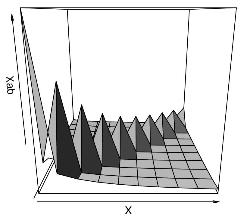
(a) Real data $\Pi^{AB}(X)$

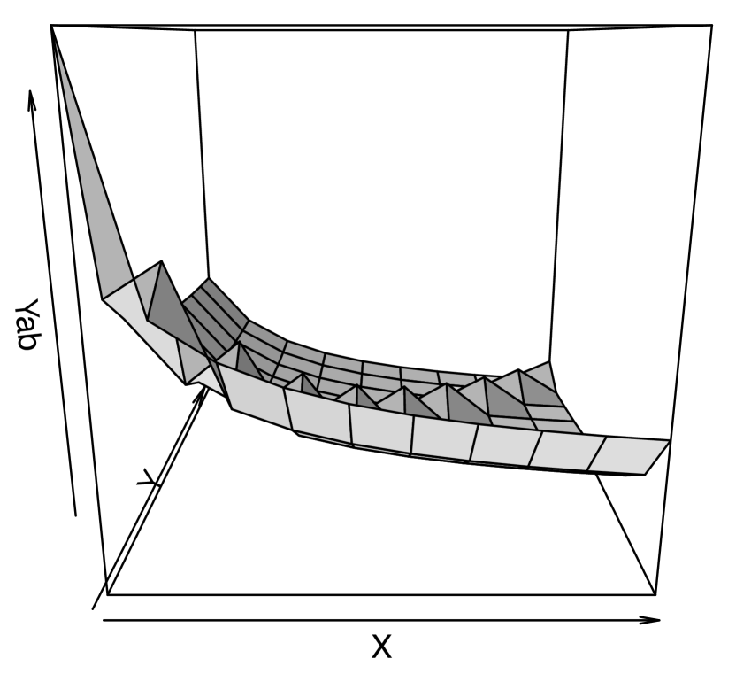
(b) Perturbed $\lambda^{AB}(Y)$

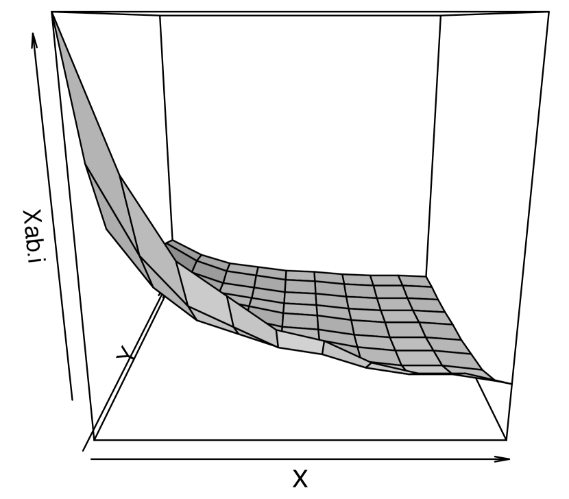
(c) Estimated $\hat{\Pi}^{AB}_{\sf RRInd}(X)$

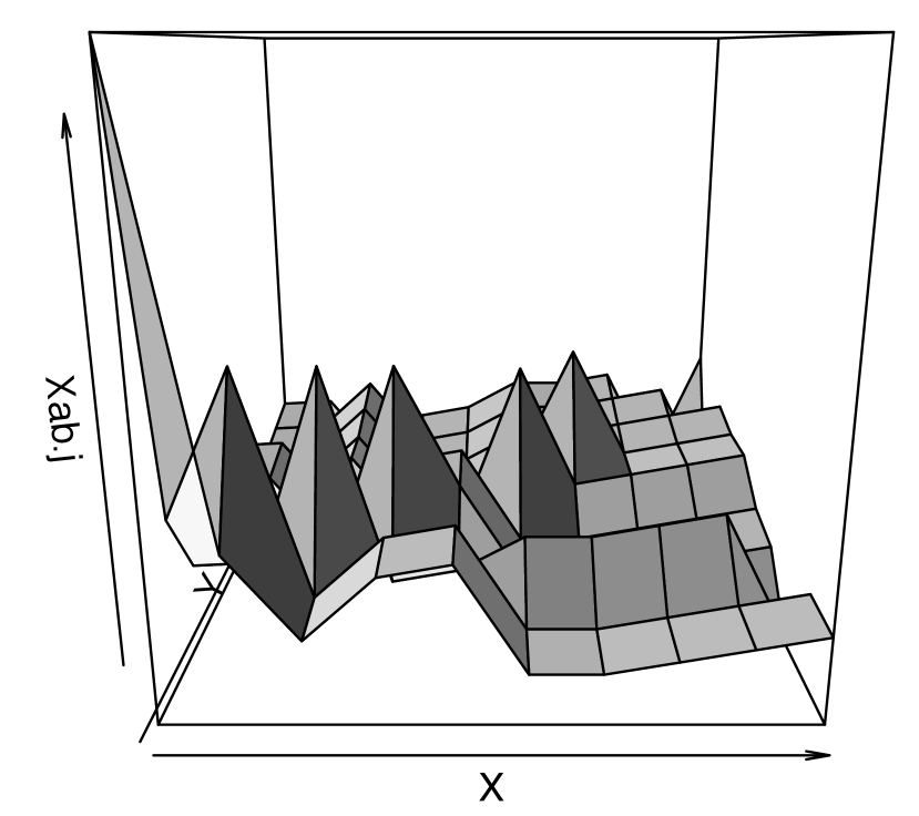
(d) Estimated $\hat{\Pi}^{AB}_{\sf RRIndJoint}(X)$

Figure 9: Example of a 2-way joint probability distribution, with estimated distributions for RR-Independent and RR-Ind-Joint

-D2 Results (Synthetic Data)

Figures 10 shows synthetic-data MAE values for four sets of parameter values, namely, Cramer’s V statistics $v\in[0,1]$, Privacy budget $\epsilon=0.1,\ldots,2$, Number of individuals $n=10,100,1000,10000$, and Domain sizes (the number of unique values in attribute) $d(=|\Omega_{A}|=|\Omega_{B}|)=2,\ldots,20$.

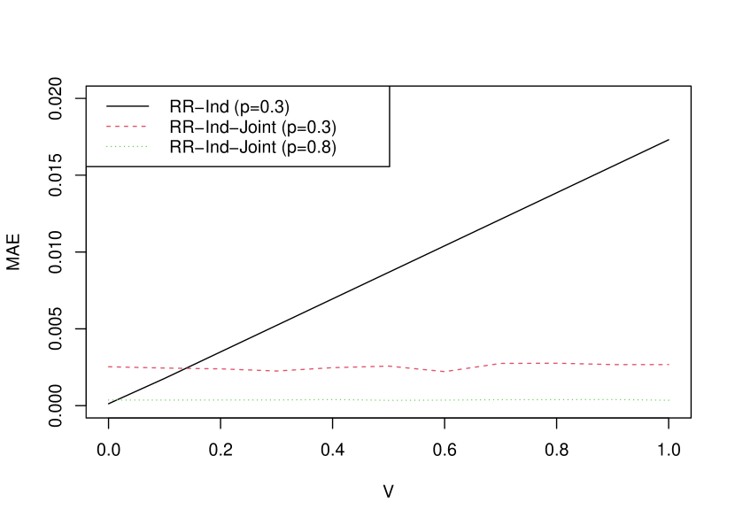
(a) Correlation $v$

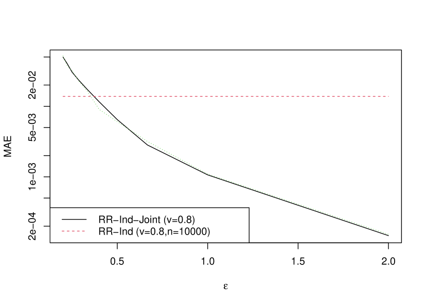
(b) Privacy budget $\epsilon$

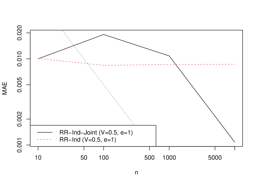
(c) Number of respondents $n$

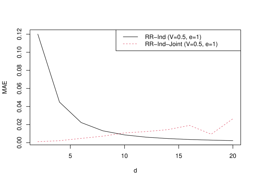
(d) Domain size $d(=|A|)$

Figure 10: Synthetic-data MAEs

Figure 10(a) shows that the estimation error for RR-Independent depends on the correlation between attributes. The MAE is proportional to $V$ with two extreme cases: 0 when $A$ and $B$ are independent ($V=0$) and the highest value when $A$ completely depends on $B$ ($V=1$). RR-Independent estimates the joint probability, via the product of two marginal probabilities, as $\hat{\Pi}^{AB}(a,b)=\hat{\sigma}^{A}(a)\hat{\sigma}^{B}(b)$, under the assumption of independent attributes, for which $V=0$. The estimation error is therefore linear in $V$ (i.e., is considered as the ratio of independent pairs of values $(a,b)$ to the $d\times d$ pairs). In contrast, the MAE for RR-Ind-Joint does not depend on $V$. It estimates the joint probabilities accurately, irrespective of any attributes correlations.

Figure 10(b) shows that the MAE of RR-Ind-Joint decreases as the privacy budget $\epsilon$ increases, which follows in turn the increases in the probabilities of retaining. It also shows that the MAE for RR-Independent is constant because the primary part of the estimation error is caused by the strength of correlation between attributes and the effect of the privacy budget is to hide the other errors.

The MAE for RR-Ind-Joint depends on the number of respondents $n$ and the domain size $d=|A|$. There is a reduction in MAE with decreasing $n$ in Fig. 10(c). The MAE of RR-Ind-Joint decreases according to $1/n$ when $n>1000$. The MAE also tends to increase with increasing $d$ in Fig. 10(d). We conclude that RR-Ind-Joint estimation needs a sufficiently large number of respondents and has a limit of the dimensionality.

The reduction of MAE with increasing $d$ is consistent with Theorem 4, which states that the MAE is linear with respect to $1/\sqrt{d}$.

-E Continuous attribute

Continuous data can be quantified into several categories if necessary. Fig. 11 shows the frequency distributions of Male (light) and Female (dark) respondents and for Age (categorized into 20-year bins (Fig. 11(a))), the frequency distributions performed via RR(X) (Fig. 11(b)) , and the estimated distributions via RR-Independent (Fig. 11(c)) and via RR-Ind-Joint (Fig. 11(d)). The estimations for RR-Ind-Joint are close to the original distribution $\Pi$.

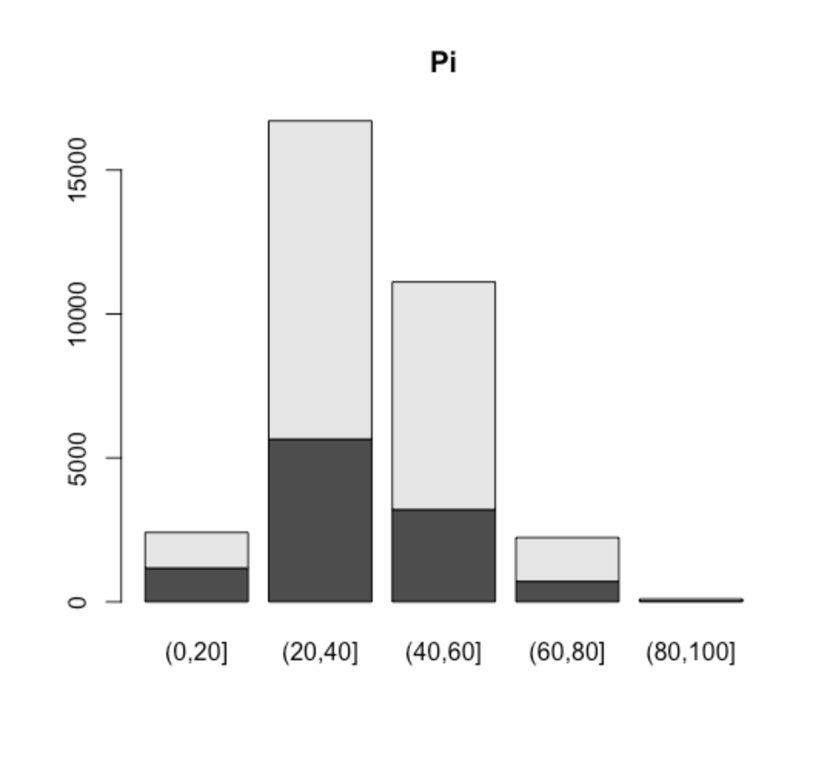
(a) Histogram for Age and Sex

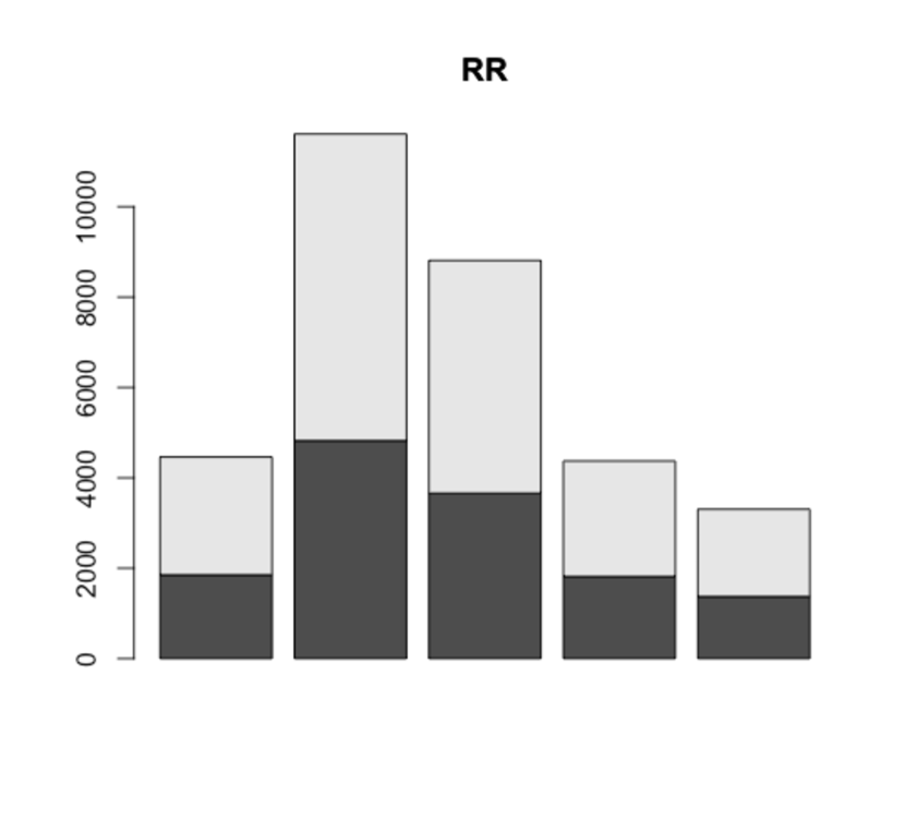
(b) Randomized $Y$

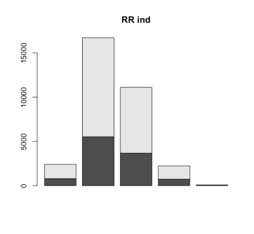
(c) Estimated $\hat{\Pi}_{\sf RRInd}^{S}$

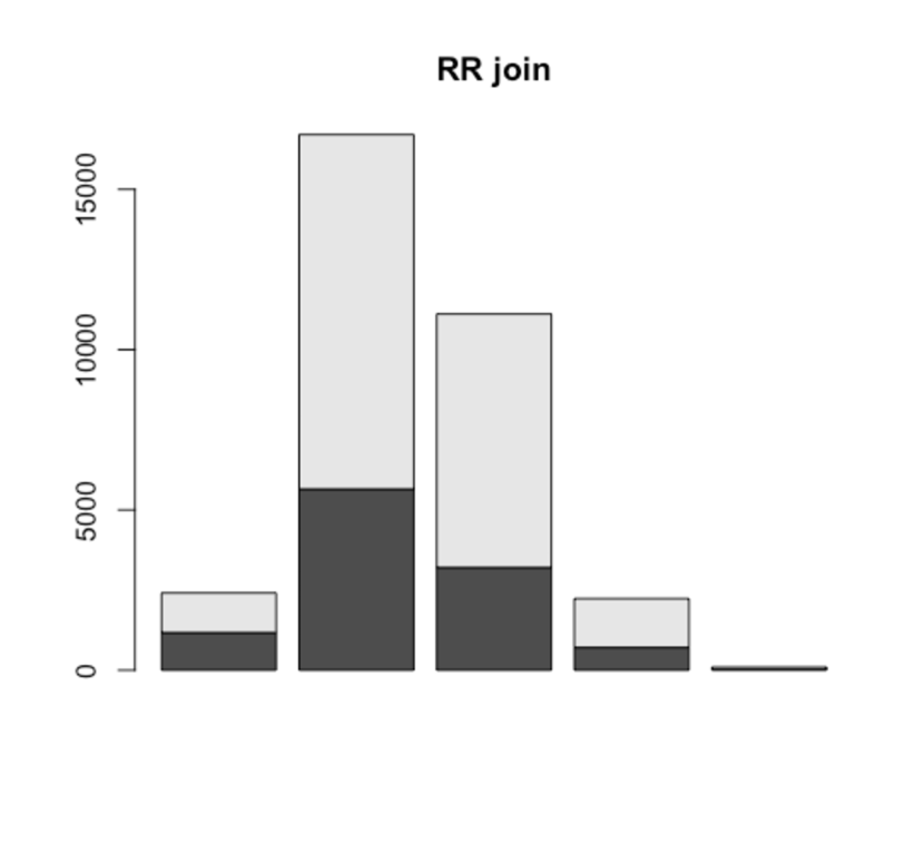
(d) Estimated $\hat{\Pi}_{\sf RRIndJoint}^{S}$

Figure 11: Examples of continuous attribute Age and nominal attribute Sex

-F Code availability

The source code of RR-Ind-Joint in R is available at ().

References

- [1] Pedro F. Saint-Maurice, et al. “Association of Daily Step Count and Step Intensity With Mortality Among US Adults,” JAMA, 323(12) pp.1151-1160, 2020.
- [2] H. Shen, M. Zhang, and J. Shen, “Efficient privacy-preserving cubedata aggregation scheme for smart grids,” IEEE Trans. Inf. Forensics and Security, vol. 12, no. 6, pp. 1369-1381, 2017.
- [3] J. Domingo-Ferrer and J. Soria-Comas, “Multi-Dimensional Randomized Response,” in IEEE Transactions on Knowledge and Data Engineering, 2022, doi:10.1109/TKDE.2020.3045759.
- [4] X. Ren et al., “LoPub : High-Dimensional Crowdsourced Data Publication With Local Differential Privacy,” in IEEE Transactions on Information Forensics and Security, vol. 13, no. 9, pp. 2151-2166, Sept. 2018, doi:10.1109/TIFS.2018.2812146.
- [5] Teng Wang, Xinyu Yang, Xuebin Ren, Wei Yu, and Shusen Yang, “Locally private high-dimensional crowdsourced data release based on copula functions,” IEEE Transactions on Services Computing, pp. 1-1, 2019.
- [6] Xue Jiang, Xuebing Zhou, Jens Grossklags, “Privacy-Preserving High-dimensional Data Collection with Federated Generative Autoencoder”, Proceedings on Privacy Enhancing Technologies, pp. 481-500, 2022. DOI:10.2478/popets-2022-0024
- [7] Ilya Tolstikhin, Olivier Bousquet, Sylvain Gelly, and Bernhard Scholkopf, “Wasserstein auto-encoders,” In International Conference on Learning Representations (ICLR 2018), Vancouver, BC, Canada, 2018.
- [8] H. Cramér, Mathematical Methods of Statistics, Princeton University Press, 1946.
- [9] Q. Ye, H. Hu, X. Meng, H. Zheng, “PrivKV : Key-Value Data Collection with Local Differential Privacy”, IEEE S&P, pp. 294-308, 2019.
- [10] C. Dwark, F. McSherry, K. Nissim, A. Smith, “Calibrating noise to sensitivity in private data analysis,” TCC, Vol. 3876, p. 265-284, 2006.
- [11] J. C. Duchi, M. I. Jordan, M. J. Wainwright, “Local privacy and statistical minimax rates,” FOCS, pp. 429-438, 2013.
- [12] P. Kairouz, S. Oh, and P. Viswanat, “Extremal mechanisms for local differential privacy”, NIPS, pp. 2879-2887, 2014.
- [13] S. L. Warner, “Randomized response: A survey technique for eliminating evasive answer bias”, Journal of the American Statistical Association, pp. 63-69, 1965.
- [14] T. T. Nguyên, X. Xiao, Y. Yang, S. C. Hui, H. Shin, J. Shin, “Collecting and analyzing data from smart device users with local differential privacy”, arXiv:1606.05053, 2016.
- [15] F. McSherry, “Privacy integrated queries: An extensible platform for privacy-preserving data analysis”, SIGMOD, pp. 19-30, 2009.
- [16] Úlfar Erlingsson, Vasyl Pihur, Aleksandra Korolova, “RAPPOR: Randomized Aggregatable Privacy-Preserving Ordinal Response”, ACM Conference on Computer and Communications Security, pp.1054-1067, 2014.
- [17] “Learning with Privacy at Scale” https://machinelearning.apple.com/2017/12/06/learning-with-privacy-at-scale.html (accessed on 2019).
- [18] Kairouz, P., Oh, S., Viswanath, P., “The Composition Theorem for Differential Privacy” Proceedings of the 32nd International Conference on Machine Learning, 37, pp. 1376-1385, 2015.
- [19] C. Dwork and A. Roth, “The algorithmic foundations of differential privacy”, Found. Trends Theor. Comput. Sci. 9, 3-4, 211-407, 2014.
- [20] V. Strassen, “Gaussian elimination is not optimal”, Numerische Mathematik, 13(4), pp. 354-356, 1969.
- [21] K. Bache and M. Lichman, UCI Machine Learning Repository, 2013. https://archive.ics.uci.edu/ml/datasets/adult
- [22] Meek, Thiesson, and Heckerman, “The Learning Curve Method Applied to Clustering”, The Journal of Machine Learning Research, 2011. https://archive.ics.uci.edu/ml/datasets/US+Census+Data+(1990)
- [23] Hans Hofmann, “Statlog (German Credit Data) Data Set”, https://archive.ics.uci.edu/ml/datasets/Statlog+%28German+Credit+Data%29
- [24] https://archive.ics.uci.edu/ml/datasets/Nursery
- [25] S. Yeom, I. Giacomelli, M. Fredrikson and S. Jha, “Privacy Risk in Machine Learning: Analyzing the Connection to Overfitting,” 2018 IEEE 31st Computer Security Foundations Symposium (CSF), pp. 268-282, 2018.
- [26] R. Shokri, M. Stronati, C. Song and V. Shmatikov, “Membership Inference Attacks Against Machine Learning Models,” 2017 IEEE Symposium on Security and Privacy (SP), pp. 3-18, 2017.
- [27] M. Fang, X. Cao, J. Jia and N. Gong, “Local Model Poisoning Attacks to Byzantine-Robust Federated Learning,” 29th USENIX Security Symposium (USENIX Security 20), pp. 1605–1622, 2020.
- [28] Y. Wang, X. Wu and D. Hu., “Using randomized response for differential privacy preserving data collection,” In Proceedings of the EDBT/ICDT 2016 Joint Conference, 2016.
- [29] T. Wang, J. Blocki, N. Li and S. Jha, “Locally differentially private protocols for frequency estimation,” In Proceedings of the 26th USENIX Security Symposium, ACM, pp. 729-745, 2017.
- [30] X. Zhang, L. Chen, K. Jin and X. Meng. Private high-dimensional data publication with junction tree. Journal of Computer Research and Development 55 (2018) 2794-2809
- [31] J. Zhang, G. Cormode, C.M. Procopiuc, D. Srivastava and X. Xiao, “PrivBayes: Private data release via Bayesian networks,” ACM Transactions on Database Systems (TODS), 42(4), pp.1-4, 2017.
- [32] Z. Zhang, T. Wang, N. Li, S. He and J. Chen, “CALM: Consistent adaptive local marginal for marginal release under local differential privacy,” In Proceedings of the 2018 ACM SIGSAC Conference on Computer and Communications Security (CCS’18), ACM, pp. 212-229, 2018.
- [33] Giulia Fanti, Vasyl Pihur, and Ulfar Erlingsson, “Building a Rappor with the unknown: Privacy-preserving learning of associations and data dictionaries,” Proceedings on Privacy Enhancing Technologies, 3:1-21, 2016.
- [34] J. C. Duchi, M. I. Jordan, and M. J. Wainwright, “Local privacy and statistical minimax rates,” in Proc. IEEE 54th Annu. Symp. Foundations Comput. Sci., pp. 429-438, 2013.
- [35] W. Qardaji, W. Yang, and N. Li, “PriView: Practical differentially private release of marginal contingency tables,” in Proc. ACM SIGMOD Int. Conf. Manage. Data, pp. 1435-1446, 2014.
- [36] B. Ding, M. Winslett, J. Han, and Z. Li, “Differentially private data cubes: Optimizing noise sources and consistency,” in Proc. ACM SIGMOD Int. Conf. Manage. Data, pp. 217-228, 2011.
- [37] R. Chen, Q. Xiao, Y. Zhang, and J. Xu, “Differentially private high-dimensional data publication via sampling-based inference,” in Proc. 21th ACM SIGKDD Int. Conf. Knowl. Discovery Data Mining, pp. 129-138, 2015.
- [38] C. Xu, J. Ren, Y. Zhang, Z. Qin, and K. Ren, “DPPro: Differentially private high-dimensional data release via random projection,” IEEE Trans. Inf. Forensics Security, vol. 12, no. 12, pp. 3081-3093, 2017.
- [39] Wahbeh H. Qardaji and Weining Yang and Ninghui Li, “Understanding Hierarchical Methods for Differentially Private Histograms,” in Proc. VLDB Endow., Vol. 6, pp. 1954-1965, 2013.
- [40] W. Day and N. Li, “Differentially private publishing of high-dimensional data using sensitivity control,” in Proc. ASIACCS, pp. 451-462, 2015.
- [41] R. Bassily and A. SmithLi, “Local, private, efficient protocols for succinct histograms,” in Proc. ACM STOC, pp. 127-135, 2015.
- [42] Z. Qin, Y. Yang, T. Yu, I. Khalil, X. Xiao, and K. Ren, “Heavy hitter estimation over set-valued data with local differential privacy,” in Proc. ACM CCS, pp. 192-203, 2016.
- [43] Jordi Soria-Comas, Josep Domingo-Ferrer, “Optimal data-independent noise for differential privacy,” Information Sciences, Volume 250, pp. 200-214, 2013.
- [44] Wang, Ning and Xiao, Xiaokui and Yang, Yin and Zhao, Jun and Hui, Siu Cheung and Shin, Hyejin and Shin, Junbum and Yu, Ge, “Collecting and Analyzing Multidimensional Data with Local Differential Privacy,” 2019 IEEE 35th International Conference on Data Engineering (ICDE), pp. 638-649, 2019.
- [45] Wang T, Lopuhaa-Zwakenberg M, Li Z, Skoric B, Li N., “Locally Differentially Private Frequency Estimation with Consistency,” In NDSS 2020, 2020.
- [46] Heber H. Arcolezi, Jean-Francois Couchot, Bechara Al Bouna, and Xiaokui Xiao, “Random Sampling Plus Fake Data: Multidimensional Frequency Estimates With Local Differential Privacy,” In Proceedings of the 30th ACM International Conference on Information & Knowledge Management (CIKM ’21), ACM, pp. 47-57, 2021.
- [47] Graham Cormode, Tejas Kulkarni, and Divesh Srivastava, “Marginal Release Under Local Differential Privacy,” In Proceedings of the 2018 International Conference on Management of Data (SIGMOD ’18), ACM, pp.131-146, 2018.