A simple extension of Azadkia & Chatterjee’s rank correlation to a vector of endogenous variables

Abstract

We propose a direct and natural extension of Azadkia & Chatterjee’s rank correlation $T$ introduced in [4] to a set of $q\geq 1$ endogenous variables. The approach builds upon converting the original vector-valued problem into a univariate problem and then applying the rank correlation $T$ to it. The novel measure $T^{q}$ then quantifies the scale-invariant extent of functional dependence of an endogenous vector $\mathbf{Y}=(Y_{1},\dots,Y_{q})$ on a number of exogenous variables $\mathbf{X}=(X_{1},\dots,X_{p})$, $p\geq 1$, characterizes independence of $\mathbf{X}$ and $\mathbf{Y}$ as well as perfect dependence of $\mathbf{Y}$ on $\mathbf{X}$ and hence fulfills all the desired characteristics of a measure of predictability. Aiming at maximum interpretability, we provide various general invariance and continuity conditions for $T^{q}$ as well as novel ordering results for conditional distributions, revealing new insights into the nature of $T$. Building upon the graph-based estimator for $T$ in [4], we present a non-parametric estimator for $T^{q}$ that is strongly consistent in full generality, i.e., without any distributional assumptions. Based on this estimator we develop a model-free and dependence-based feature ranking and forward feature selection of multiple-outcome data, and establish tools for identifying networks between random variables. Real case studies illustrate the main aspects of the developed methodology.

and

1 Introduction

In regression analysis the main objective is to estimate the functional relationship $\mathbf{Y}=f(\mathbf{X},\bm{\varepsilon})$ between a set of $q\geq 1$ endogenous variables $\mathbf{Y}=(Y_{1},\dots,Y_{q})$ and a set of $p\geq 1$ exogenous variables $\mathbf{X}=(X_{1},\dots,X_{p})$ where $\bm{\varepsilon}$ is a model-dependent error. In view of constructing a good model, the question naturally arises to what extent $\mathbf{Y}$ can be predicted from the information provided by the multivariate exogenous variable $\mathbf{X}$, and which of the exogenous variables are relevant for the model at all.

We refer to $\kappa$ as a measure of predictability for the $q$-dimensional random vector $\mathbf{Y}$ given the $p$-dimensional random vector $\mathbf{X}$ if it satisfies the following axioms (cf, e.g., [6, 22, 41, 78] for the case $q=1$):

1. $0\leq\kappa(\mathbf{Y}|\mathbf{X})\leq 1$.

2. $\kappa(\mathbf{Y}|\mathbf{X})=0$ if and only if $\mathbf{Y}$ and $\mathbf{X}$ are independent.

3. $\kappa(\mathbf{Y}|\mathbf{X})=1$ if and only if $\mathbf{Y}$ is perfectly dependent on $\mathbf{X}$, i.e., there exists some measurable function ${\bf f}:\mathbb{R}^{p}\to\mathbb{R}^{q}$ such that $\mathbf{Y}={\bf f}(\mathbf{X})$ almost surely.

In addition to the above-mentioned three axioms, it is desirable that additional information improves the predictability of $\mathbf{Y}\,.$ This yields the following two closely related properties of a measure of predictability $\kappa$ which prove to be of utmost importance for this paper (cf, e.g, [35, 39]):

1. Information gain inequality: $\kappa(\mathbf{Y}|\mathbf{X})\leq\kappa(\mathbf{Y}|(\mathbf{X},\mathbb{Z}))$ for all $\mathbf{X}$, $\mathbb{Z}$ and $\mathbf{Y}$.

2. Characterization of conditional independence: $\kappa(\mathbf{Y}|\mathbf{X})=\kappa(\mathbf{Y}|(\mathbf{X},\mathbb{Z}))$ if and only if $\mathbf{Y}$ and $\mathbb{Z}$ are conditionally independent given $\mathbf{X}$.

Due to axioms (A2) and (A3), the values $0$ and $1$ of a measure of predictability $\kappa$ have a clear interpretation. However, the meaning of $\kappa\,,$ taking values in the interval $(0,1)\,,$ is not specified. This justifies the investigation of dependence orderings $\prec$ that are compatible with $\kappa$ in the following sense:

1. Monotonicity: If $(\mathbf{X},\mathbf{Y})\prec(\mathbf{X}^{\prime},\mathbf{Y}^{\prime})$, then $\kappa(\mathbf{Y}|\mathbf{X})\leq\kappa(\mathbf{Y}^{\prime}|\mathbf{X}^{\prime})$.

In view of interpreting the values of a measure of predictability $\kappa$, it is further desirable to have an understanding of the measures’ performance in terms of convergence, such as

1. Continuity: If $(\mathbf{X}_{n},\mathbf{Y}_{n})_{n\in\mathbb{N}}$ converges (in some sense) to $(\mathbf{X},\mathbf{Y})$, then $\lim_{n\to\infty}\kappa(\mathbf{Y}_{n}|\mathbf{X}_{n})=\kappa(\mathbf{Y}|\mathbf{X})$.

To the best of the authors’ knowledge, so far the only measure of predictability applicable to a vector $\mathbf{Y}=(Y_{1},\dots,Y_{q})$ of $q\geq 1$ endogenous variables has been introduced by Deb, Ghosal and Sen [22] and employs the vector-valued structure of $\mathbf{Y}$ for its evaluation. In contrast to that, in the present paper, we take a different approach by converting the original vector-valued problem into a univariate problem and then applying to it a measure of predictability for a single endogenous variable capable of characterizing conditional independence. A particularly suitable candidate for such a measure has been recently introduced by Azadkia and Chatterjee [4]: Their so-called ‘simple measure of conditional dependence’ $T$ is given (in its unconditional form) by

$$T(Y|\mathbf{X}):=\frac{\int_{\mathbb{R}}{\rm var}(P(Y\geq y\,|\,\mathbf{X}))\;\mathrm{d}P^{Y}(y)}{\int_{\mathbb{R}}{\rm var}(\mathds{1}_{\{Y\geq y\}})\;\mathrm{d}P^{Y}(y)}$$ (1)

and is based on Chatterjee [14] and Dette, Siburg and Stoimenov [23]. It is also known as Dette-Siburg-Stoimenov’s dependence measure and attracted a lot of attention in the past few years; see, e.g., [3, 6, 11, 22, 40, 44, 55, 74, 78, 89]. The measure $T$ captures the variability of the conditional distributions in various ways and thus quantifies the scale-invariant extent of functional (or monotone regression) dependence of the single endogenous variable $Y$ (i.e., $q=1$) on the exogenous variables $X_{1},\dots,X_{p}$, and fulfills the above-mentioned characteristics of a measure of predictability for a single endogenous variable.

A naive way of extending $T$ to a measure of predictability for a vector $(Y_{1},\dots,Y_{q})$ of $q\geq 1$ endogenous variables is to sum up the individual amounts of predictability, namely, to consider the quantity

$$T^{\Sigma}(\mathbf{Y}|\mathbf{X}):=\frac{1}{q}\sum_{i=1}^{q}T(Y_{i}|\mathbf{X}).$$ (2)

It is clear that $T^{\Sigma}$ satisfies axioms (A1) and (A3) of a measure of predictability. However, it fails to characterize independence between the vectors $\mathbf{X}$ and $\mathbf{Y}$ (even though $\mathbf{X}$ and $Y_{i}$ are independent for every $i\in\{1,\dots,q\}$); for an illustration, consider a random vector $(X,Y_{1},Y_{2})$ with pairwise independent marginals and assume that the vector is globally dependent (for instance, consider a random vector whose dependence structure coincides with the cube copula presented in Example 2.9, see also [61, Example 3.4.], or an EFGM copula [28]). Then $T^{\Sigma}((Y_{1},Y_{2})|X)=0$ even though the random quantities $X$ and $(Y_{1},Y_{2})$ are dependent.

Although the recent literature is rich concerning measures of predictability for a single endogenous variable (see, e.g., [32, 39, 45, 78, 84]), the measure $T$ is special in that it not only satisfies the information gain inequality (P1) (like, for instance, the measure discussed in [39]) but also characterizes conditional independence (P2), see [4, Lemma 11.2]. Using these properties, we show that the functional $T^{q}$ defined by

$$T^{q}(\mathbf{Y}|\mathbf{X}) :=\frac{\sum_{i=1}^{q}\big{[}T(Y_{i}|(\mathbf{X},Y_{i-1},\dots,Y_{1}))-T(Y_{i}|(Y_{i-1},\dots,Y_{1}))\big{]}}{\sum_{i=1}^{q}\big{[}1-T(Y_{i}|(Y_{i-1},\dots,Y_{1}))\big{]}}$$ (3)

$$\phantom{:}=1-\frac{q-\sum_{i=1}^{q}T(Y_{i}|(\mathbf{X},Y_{i-1},\dots,Y_{1}))}{q-\sum_{i=1}^{q}T(Y_{i}|(Y_{i-1},\dots,Y_{1}))}\,,$$ (4)

$$\text{with}~{}~{}~{}T(Y_{1}|\emptyset) :=0\,,$$ (5)

is a natural extension of Azadkia & Chatterjee’s rank correlation coefficient to a measure of predictability for a vector $(Y_{1},\dots,Y_{q})$ of $q\geq 1$ endogenous variables. To illustrate that $T^{q}$ is the correct choice for such an extension, we first observe that for $q=1$ the above defined functional $T^{q}$ reduces to $T\,.$ Further, due to the information gain inequality for $T\,,$ each summand of the nominator in (3) is non-negative. Since $T$ characterizes conditional independence, the $i$-th summand of the nominator vanishes if and only if $Y_{i}$ and $\mathbf{X}$ are conditionally independent given $(Y_{i-1},\ldots,Y_{1})\,.$ Hence, as a consequence of the chain rule for conditional independence, $\mathbf{X}$ and $\mathbf{Y}$ are independent if and only if $T^{q}(\mathbf{Y}|\mathbf{X})=0\,.$ The denominator, which only takes values in the interval $[1,q]\,,$ guarantees that $T^{q}$ is normalized.

Our paper contributes to the literature in the following way:

1. $T^{q}$ defined by (3) is a measure of predictability for $\mathbf{Y}$ given $\mathbf{X}\,,$ where $T^{q}$ exhibits a simple expression, is fully non-parametric, has no tuning parameters and is well-defined without any distributional assumptions. Further, $T^{q}$ fulfills the information gain inequality (P1), characterizes conditional independence (P2), satisfies the so-called data processing inequality (see, e.g., [17]), is self-equitable (cf, e.g., [53]), and exhibits numerous invariance properties, see Section 2.

2. To tackle the monotonicity property (P3), we introduce the Schur order for conditional distributions $\leq_{S}$ in Section 3.1, which turns out to be a natural ordering of predictability hidden behind the properties of $T\,.$ All the fundamental properties of $\leq_{S}\,,$ i.e., the characterization of (conditional) independence and complete directed dependence as well as the information gain inequality, are inherited by $T\,.$ Exploiting the derived characteristics of $\leq_{S}\,,$ a novel class of measures of predictability for $\mathbf{Y}$ given $\mathbf{X}$ is constructed and the specificity of $T^{q}$ within this class is discussed, see Section 7.

3. To address the continuity property (P4), a general continuity results for $T^{q}$ is given in Section 4 using a characterization of conditional weak convergence established in [80]. Applying these results, continuity of $T^{q}$ in classes of elliptical and $l_{1}$-norm symmetric distributions is studied in Section 4. For elliptical distributions, a characterization is given for the case where $T^{q}$ attains the values 0 and 1, respectively, see Section 3.2.

4. $T^{q}$ has a model-free, strongly consistent estimator which can be computed in $O(n\log n)$ time and which is given by a simple function of Azadkia & Chatterjee’s graph-based estimator $T_{n}$ for $T$. Adapting the ideas by Lin and Han [55], asymptotical normality is shown for a version of the estimator for $T^{\Sigma}$ defined by (2), see Section 5.

5. As important applications, Section 6 presents a model-free and dependence-based feature ranking and forward feature selection of data with multiple outcomes, thus facilitating the identification of the most relevant explanatory variables. Further, a hierarchical clustering method for random variables is established and a visualization of the interconnectedness of random variables based on the degree of predictability among them is proposed. Various real data examples from medicine, meteorology and finance demonstrate $T^{q}$’s broad applicability.

The paper concludes with a geometric illustration of the most important properties of the measure $T$ and the construction principle underlying $T^{q}$ (Section 8). All proofs are deferred to the appendix.

Throughout the paper, we assume that $\mathbf{X}=(X_{1},\ldots,X_{p})\,,$ $\mathbf{Y}=(Y_{1},\ldots,Y_{q})\,,$ and $\mathbb{Z}=(Z_{1},\ldots,Z_{r})$ are $p$-, $q$-, and $r$-dimensional random vectors, respectively, defined on a common probability space $(\Omega,\mathcal{A},P)\,,$ with $p,q,r\in\mathbb{N}$ being arbitrary. Variables not in bold type refer to one-dimensional real-valued quantities. We denote $\mathbf{Y}$ as the endogenous random vector which is always assumed to have non-degenerate components, i.e., for all $i\in\{1,\ldots,q\}\,,$ the distribution of $Y_{i}$ does not follow a one-point distribution. This equivalently means that $\mathrm{Var}(Y_{i})>0\,,$ which ensures that $T(Y_{i}|\,\cdot\,)$ in (1) and, hence, $T^{q}(\mathbf{Y}|\,\cdot\,)$ in (3) are well-defined. Note that the assumption of non-degeneracy is inevitable because, otherwise, $Y_{i}$ is constant and thus both independent from $\mathbf{X}$ and a function of $\mathbf{X}\,.$ However, in this case, there is no measure satisfying both the axioms (A2) and (A3).

2 Properties of the extension $T^{q}$

In this section, various basic properties of the measure $T^{q}$ are established. The first part focuses on the fundamental characteristics, showing that $T^{q}$ satisfies axioms (A1) to (A3) as well as properties (P1) and (P2). Then the so-called data processing inequality as well as self-equitability of $T^{q}$ are discussed and several important invariance properties are derived. Finally, it is shown that the measure $T$ is invariant with respect to a dimension reduction principle preserving the key information about the extent of functional dependence of the endogenous variables on the exogenous vector–a principle that is used in the subsequent sections.

2.1 Fundamental properties of $T^{q}$

As a first main result, the following theorem states that $T^{q}$ in (3) satisfies all the desired axioms (A1) to (A3) and hence can be viewed as a natural extension of Azadkia & Chatterjee’s rank correlation coefficient to a measure of predictability for a vector $(Y_{1},\dots,Y_{q})$ of endogenous variables:

Theorem 2.1 ($T^{q}$ as a measure of predictability).

The map $T^{q}$ defined by (3) satisfies the axioms (A1) to (A3) of a measure of predictability, i.e.,

1. $T^{q}(\mathbf{Y}|\mathbf{X})\in[0,1]\,,$

2. $T^{q}(\mathbf{Y}|\mathbf{X})=0$ if and only if $\mathbf{X}$ and $\mathbf{Y}$ are independent,

3. $T^{q}(\mathbf{Y}|\mathbf{X})=1$ if and only if $\mathbf{Y}$ is perfectly dependent on $\mathbf{X}$.

By the following result, not only $T$ but also $T^{q}$ fulfills the information gain inequality (P1) and characterizes conditional independence (P2):

Theorem 2.2 (Information gain inequality; conditional independence).

The map $T^{q}$ defined by (3)

1. fulfills the information gain inequality (P1), i.e., $T^{q}(\mathbf{Y}|\mathbf{X})\leq T^{q}(\mathbf{Y}|(\mathbf{X},\mathbb{Z}))$ for all $\mathbf{X}$, $\mathbb{Z}$ and $\mathbf{Y}$,

2. characterizes conditional independence (P2), i.e., $T^{q}(\mathbf{Y}|\mathbf{X})=T^{q}(\mathbf{Y}|(\mathbf{X},\mathbb{Z}))$ if and only if $\mathbf{Y}$ and $\mathbb{Z}$ are conditionally independent given $\mathbf{X}$.

From Theorem 2.2 it immediately follows that $T^{q}$ fulfills the so-called data processing inequality which involves that a transformation of the explanatory variables cannot enhance the degree of predictability; see [17] for a detailed discussion.

Corollary 2.3 (Data processing inequality).

The map $T^{q}$ defined by (3) fulfills the data processing inequality, i.e.,

$$T^{q}(\mathbf{Y}|\mathbb{Z})\leq T^{q}(\mathbf{Y}|\mathbf{X})$$

for all $\mathbf{X},\mathbf{Y},\mathbb{Z}$ such that $\mathbf{Y}$ and $\mathbb{Z}$ are conditionally independent given $\mathbf{X}$. In particular,

$$T^{q}(\mathbf{Y}|{\bf h}(\mathbf{X}))\leq T^{q}(\mathbf{Y}|\mathbf{X})$$ (6)

for all $\mathbf{X},\mathbf{Y}$ and all measurable functions ${\bf h}$.

The data processing inequality implies several interesting invariance properties for $T^{q}$. The first one is the so-called self-equitability introduced in [53] (see also [25]). According to [67] self-equitability states that “the statistic should give similar scores to equally noisy relationships of different types”. In a regression setting $\mathbf{Y}={\bf f}(\mathbf{X})+\bm{\varepsilon}$ it means that the measure of predictability $T^{q}$ “depends only on the strength of the noise $\bm{\varepsilon}$ and not on the specific form of ${\bf f}$” [78].

Corollary 2.4 (Self-equitability).

The map $T^{q}$ defined by (3) is self-equitable, i.e.,

$$T^{q}(\mathbf{Y}|{\bf h}(\mathbf{X}))=T^{q}(\mathbf{Y}|\mathbf{X})$$

for all $\mathbf{X}$, $\mathbf{Y}$ and all measurable functions ${\bf h}$ such that $\mathbf{Y}$ and $\mathbf{X}$ are conditionally independent given ${\bf h}(\mathbf{X})$.

2.2 Distributional invariance

We make use of the data processing inequality to gain insight into some important invariance properties of $T^{q}(\mathbf{Y}|\mathbf{X})$ concerning the distributions of $\mathbf{X}$ and $\mathbf{Y}\,.$

Let $\mathbb{V}=(V_{1},\ldots,V_{p})$ be a random vector (on $(\Omega,\mathcal{A},P)$ which is assumed to be non-atomic) that is independent of $\mathbf{X}=(X_{1},\ldots,X_{p})$ and uniformly on $(0,1)^{p}$ distributed. Then the multivariate distributional transform $\tau_{\mathbf{X}}(\mathbf{X},\mathbb{V})$ of $\mathbf{X}$ is defined by

$$\tau_{\mathbf{X}}(\mathbb{x},\bm{\lambda}):=\big{(}F_{1}(x_{1},\lambda_{1}),F_{2}(x_{2},\lambda_{2}|x_{1})\dots,F_{p}(x_{p},\lambda_{p}|x_{1},\dots,x_{p-1})\big{)}$$

for $\mathbb{x}=(x_{1},\ldots,x_{p})\in\mathbb{R}^{p}$ and all $\bm{\lambda}=(\lambda_{1},\ldots,\lambda_{p})\in[0,1]^{p}$, where

$$F_{1}(x_{1},\lambda_{1}) := P(X_{1}<x_{1})+\lambda_{1}\,P(X_{1}=x_{1})$$

$$F_{i}(x_{i},\lambda_{i}|x_{1},\dots,x_{i-1}) := P(X_{i}<x_{i}|X_{1}=x_{1},\dots,X_{i-1}=x_{i-1})$$

$$+\lambda_{i}\,P(X_{i}=x_{i}|X_{1}=x_{1},\dots,X_{i-1}=x_{i-1})\,,\quad i\in\{2,\ldots,p\}\,.$$

For $p=1$ and for a random variable $X$ with continuous distribution function $F_{X}\,,$ the distributional transform $\tau_{X}(X,V)$ simplifies to $F_{X}(X)\,,$ which is uniformly on $(0,1)$ distributed.

As an inverse transformation of $\tau_{\mathbf{X}}\,,$ for a random vector $\mathbb{U}=(U_{1},\ldots,U_{p})$ uniformly on $(0,1)^{p}$ distributed, the multivariate quantile transform $q_{\mathbf{X}}(\mathbb{U}):=(\xi_{1},\ldots,\xi_{p})$ is defined by

$$\xi_{1} :=F_{X_{1}}^{-1}(U_{1})\,,$$ (7)

$$\xi_{i} :=F^{-1}_{X_{i}|X_{i-1}=\xi_{i-1},\ldots,X_{1}=\xi_{1}}(U_{i})~{}~{}~{}\text{for all }i\in\{2,\ldots,p\}$$ (8)

where $F_{W|\mathbb{Z}=\mathbb{z}}$ denotes the conditional distribution function of $W$ given $\mathbb{Z}=\mathbb{z}$, and $F_{Z}^{-1}$ denotes the generalized inverse function of $F_{Z}$, i.e., $F_{Z}^{-1}(u):=\inf\{z\in\mathbb{R}\,:\,F_{Z}(z)\geq u\}$.

According to [2, 65, 69, 71],

$$\tau_{\mathbf{X}}(\mathbf{X},\mathbb{V}) \text{ is a random vector that is uniformly on }(0,1)^{p}\text{ distributed,}$$ (9)

$$q_{\mathbf{X}}(\mathbb{U}) \text{ is a random vector with distribution function }F_{\mathbf{X}},$$ (10)

and the multivariate quantile transform is inverse to the multivariate distributional transform, i.e.,

$$\mathbf{X}=q_{\mathbf{X}}\big{(}\tau_{\mathbf{X}}(\mathbf{X},\mathbb{V})\big{)}\qquad P\text{-almost surely.}$$ (11)

The following result shows that the value $T^{q}(\mathbf{Y}|\mathbf{X})$ remains unchanged when replacing the exogenous variables $X_{1},\dots,X_{p}$ by their individual distributional transforms, i.e., the exogenous variables can be replaced by their individual ranks (where ties are broken at random). Further, the value $T^{q}(\mathbf{Y}|\mathbf{X})$ also remains unchanged when replacing the vector of exogenous variables $\mathbf{X}$ by its multivariate distributional transform and hence by a vector of independent and identically distributed random variables.

Corollary 2.5 (Distributional invariance in the exogenous variables).

The map $T^{q}$ defined by (3) fulfills

$$T^{q}(\mathbf{Y}|\mathbf{X})=T^{q}\big{(}\mathbf{Y}|(F_{X_{1}}(X_{1}),\dots,F_{X_{p}}(X_{p})\big{)}.$$

Further, assume that $\mathbf{Y}$ and $\mathbb{V}$ are conditionally independent given $\mathbf{X}$. Then

1. $T^{q}(\mathbf{Y}|\mathbf{X})=T^{q}(\mathbf{Y}|\tau_{\mathbf{X}}(\mathbf{X},\mathbb{V}))$.

2. $T^{q}(\mathbf{Y}|\mathbf{X})=T^{q}\big{(}\mathbf{Y}|(\tau_{X_{1}}(X_{1},V_{1}),\dots,\tau_{X_{p}}(X_{p},V_{p}))\big{)}$.

Interestingly, and in contrast to Corollary 2.5, it turns out that $T^{q}(\mathbf{Y}|\mathbf{X})$ is not invariant with respect to the (individual) distributional transforms of $\mathbf{Y}$ but it is invariant with respect to a transformation by the individual distribution functions of $\mathbf{Y}\,.$

Corollary 2.6 (Distributional invariance in the endogenous variables).

The map $T^{q}$ defined by (3) fulfills

$$T^{q}(\mathbf{Y}|\mathbf{X})=T^{q}\big{(}(F_{Y_{1}}(Y_{1}),\dots,F_{Y_{p}}(Y_{p})|\mathbf{X}\big{)}.$$

However, $T^{q}(\mathbf{Y}|\mathbf{X})\neq T^{q}(\tau_{\mathbf{Y}}(\mathbf{Y},\mathbb{V})|\mathbf{X})$ and $T^{q}(\mathbf{Y}|\mathbf{X})\neq T^{q}((\tau_{Y_{1}}(Y_{1},V_{1}),\ldots,\tau_{Y_{q}}(Y_{q},V_{q}))|\mathbf{X})$, in general.

In Subsection 2.4 below, further invariance properties of $T^{q}$ are studied. In particular, some general conditions on functions ${\bf h}$ are given that turn (6) into an equality.

2.3 A permutation invariant version

Since Azadkia & Chatterjee’s rank correlation $T$ is a measure of directed dependence, it is not symmetric, i.e., $T(Y_{2}|Y_{1})\neq T(Y_{1}|Y_{2})$ in general. This implies that the multivariate extension $T^{q}$ is in general not invariant under permutations of the endogenous variables, i.e., $T^{q}((Y_{1},Y_{2})|\mathbf{X})\neq T^{q}((Y_{2},Y_{1})|\mathbf{X})$ in general. However, permutation invariance w.r.t. the components of $\mathbf{Y}$ can be achieved by defining the map

$$\overline{T^{q}}(\mathbf{Y}|\mathbf{X}):=\frac{1}{q!}\sum_{\bm{\sigma}\in S_{q}}T^{q}(\mathbf{Y}_{\bm{\sigma}}|\mathbf{X})\,,$$ (12)

where $S_{q}$ denotes the set of permutations of $\{1,\ldots,q\}$ and where $\mathbf{Y}_{\bm{\sigma}}:=(Y_{\sigma_{1}},\ldots,Y_{\sigma_{q}})$ for $\bm{\sigma}=(\sigma_{1},\ldots,\sigma_{q})\in S_{q}\,.$ As an immediate consequence of Theorems 2.1 & 2.2 and Corollaries 2.3 & 2.4, the permutation invariant version $\overline{T^{q}}$ defines a measure of predictability that inherits all the desired properties from $T^{q}\,.$

Corollary 2.7 ($\overline{T^{q}}$ as a measure of predictability).

The map $\overline{T^{q}}$ defined by (12)

1. satisfies the axioms (A1) to (A3) of a measure of predictability.

2. fulfills the information gain inequality (P1).

3. characterizes conditional independence (P2).

In addition, $\overline{T^{q}}$ fulfills the data processing inequality and is self-equitable.

For some special cases concerning independence, conditional independence, and perfect dependence of the endogenous variables, the measures $T^{q}$ and $\overline{T^{q}}$ attain a simplified form as follows.

Remark 2.8 (Special cases regarding the dependence structure of $\mathbf{Y}$).

1. If $Y_{1},\ldots,Y_{q}$ are independent, then

   $$T^{q}(\mathbf{Y}|\mathbf{X})=\frac{1}{q}\sum_{i=1}^{q}T(Y_{i}|(\mathbf{X},Y_{i-1},\dots,Y_{1}))\,.$$ (13)

2. If $Y_{1},\ldots,Y_{q}$ are independent and conditionally independent given $\mathbf{X}$, then

   $$T^{q}(\mathbf{Y}|\mathbf{X})=\frac{1}{q}\sum_{i=1}^{q}T(Y_{i}|\mathbf{X})=\overline{T^{q}}(\mathbf{Y}|\mathbf{X})=T^{\Sigma}(\mathbf{Y}|\mathbf{X})\,.$$ (14)

3. If $Y_{i}$ is perfectly dependent on $Y_{1}$ for all $i\in\{2,\ldots,q\}\,,$ then

   $$T^{q}(\mathbf{Y}|\mathbf{X})=T(Y_{1}|\mathbf{X})\,.$$ (15)

Example 2.9 below illustrates the difference between Statements (i) and (ii) in the above remark. Also note that Statement (iii) in Remark 2.8 is not invariant under permutations of the components of $\mathbf{Y}\,,$ i.e., if $Y_{1}$ is perfectly dependent on $Y_{2}\,,$ then $T^{q}((Y_{1},Y_{2})|\mathbf{X})\neq T(Y_{2}|\mathbf{X})$ in general.

The next example shows that $T^{\Sigma}$ defined in (2) is not a measure of predictability.

Example 2.9 ($T^{q}\neq T^{\Sigma}$).

Consider the random vector $(X,Y_{1},Y_{2})$ whose mass is distributed uniformly within the four cubes

$$\big{(}0,\tfrac{1}{2}\big{)}\times\big{(}0,\tfrac{1}{2}\big{)}\times\big{(}0,\tfrac{1}{2}\big{)} \big{(}\tfrac{1}{2},1\big{)}\times\big{(}\tfrac{1}{2},1\big{)}\times\big{(}0,\tfrac{1}{2}\big{)}$$

$$\big{(}0,\tfrac{1}{2}\big{)}\times\big{(}\tfrac{1}{2},1\big{)}\times\big{(}\tfrac{1}{2},1\big{)} \big{(}\tfrac{1}{2},1\big{)}\times\big{(}0,\tfrac{1}{2}\big{)}\times\big{(}\tfrac{1}{2},1\big{)}$$

and has no mass outside these cubes. Then $Y_{1}$ and $Y_{2}$ are independent but not conditionally independent given $X$. Additionally, $X$ and $Y_{1}$ as well as $X$ and $Y_{2}$ are independent, and hence

$$T^{q}((Y_{1},Y_{2})|X)=\frac{T(Y_{1}|X)+T(Y_{2}|(X,Y_{1}))}{2}=\frac{T(Y_{2}|(X,Y_{1}))}{2}=\frac{1}{4}>0=T^{\Sigma}((Y_{1},Y_{2})|X).$$

Consequently, $T^{\Sigma}$ does not satisfy axiom (2) and thus is not a measure of predictability.

2.4 Further invariance properties of $T^{q}$

We now examine further interesting (invariance) properties of $T^{q}$ which are partly inherited by construction from the initial measure $T\,.$ Since $T^{q}$ has a simpler form and also reflects some asymmetries, we concentrate in the sequel on properties of the measure $T^{q}$ and note that $\overline{T^{q}}$ inherits most of them.

An important property of $T^{q}(\mathbf{Y}|\mathbf{X})$ is its invariance under strictly increasing and bijective transformations of $Y_{i}$ and under bijective transformations of $\mathbf{X}$ as follows.

Theorem 2.10 (Invariance under (strictly increasing) bijective transformations).

Let $\mathbb{g}=(g_{1},\ldots,g_{q})$ be a vector of strictly increasing and bijective transformations $g_{i}\colon\mathbb{R}\to\mathbb{R}$, $i\in\{1,\ldots,q\}$, and let $\mathbb{h}$ be a bijective transformation $\mathbb{R}^{p}\to\mathbb{R}^{p}$. Then $T^{q}(\mathbb{g}(\mathbf{Y})|\mathbb{h}(\mathbf{X}))=T^{q}(\mathbf{Y}|\mathbf{X})\,.$

Theorem 2.10 implies invariance of $T^{q}$ under permutations within the conditioning vector $\mathbf{X}$. The following Proposition 2.11 and Corollary 2.12 also provide a sufficient condition on the underlying dependence structure for the invariance of $T^{q}$ under permutations within the endogenous vector $\mathbf{Y}$ using the notion of copulas.

A $d$-copula is a $d$-variate distribution function on the unit cube $[0,1]^{d}$ with uniform univariate marginal distributions. Denote by $\mathsf{Ran}(F):=\{F(x)\,|\,x\in\mathbb{R}\}$ the range of a univariate distribution function $F$ and denote by $\overline{A}$ the closure of a set $A\subset\mathbb{R}\,.$ Due to Sklar’s Theorem, the joint distribution function of $(\mathbf{X},\mathbf{Y})$ can be decomposed into its univariate marginal distribution functions and a $(p+q)$-copula $C_{\mathbf{X},\mathbf{Y}}$ such that

$$F_{\mathbf{X},\mathbf{Y}}(\mathbb{x},\mathbb{y})=C_{\mathbf{X},\mathbf{Y}}(F_{X_{1}}(x_{1}),\ldots,F_{X_{p}}(x_{p}),F_{Y_{1}}(y_{1}),\ldots,F_{Y_{q}}(y_{q}))$$ (16)

for all $(\mathbb{x},\mathbb{y})=(x_{1},\ldots,x_{p},y_{1},\ldots,y_{q})\in\mathbb{R}^{p+q}\,,$ where $C_{\mathbf{X},\mathbf{Y}}$ is uniquely determined on $\mathsf{Ran}(F_{X_{1}})\times\cdots\times\mathsf{Ran}(F_{X_{p}})\times\mathsf{Ran}(F_{Y_{1}})\times\cdots\times\mathsf{Ran}(F_{Y_{q}})$; for more background on copulas and Sklar’s Theorem we refer to [28, 64].

Proposition 2.11 (Invariance under permutations).

Assume that $C_{\mathbf{X},\mathbf{Y}_{\bm{\sigma}}}=C_{\mathbf{X},\mathbf{Y}}$ for all $\bm{\sigma}\in S_{q}$ and $\overline{\mathsf{Ran}(F_{Y_{1}})}=\cdots=\overline{\mathsf{Ran}(F_{Y_{q}})}\,.$ Then $T^{q}(\mathbf{Y}_{\sigma}|\mathbf{X})=T^{q}(\mathbf{Y}|\mathbf{X})$ for all $\bm{\sigma}\in S_{q}\,.$

A $d$-variate random vector $\mathbb{W}=(W_{1},\ldots,W_{d})$ is said to be exchangeable if $\mathbb{W}\stackrel{{\scriptstyle\mathrm{d}}}{{=}}\mathbb{W}_{\bm{\sigma}}$ for all ${\bm{\sigma}}\in S_{d}\,,$ where ’ $\stackrel{{\scriptstyle\mathrm{d}}}{{=}}$ ’ denotes equality in distribution. The following corollary is an immediate consequence of the previous result.

Corollary 2.12 (Invariance under exchangeability).

Assume that the random vector $(\mathbf{X},\mathbf{Y})$ is exchangeable. Then $T^{q}(\mathbf{Y}_{\bm{\sigma}}|\mathbf{X})=T^{q}(\mathbf{Y}|\mathbf{X})$ for all ${\bm{\sigma}}\in S_{q}\,.$

The following result characterizes independence of the random vectors $\mathbf{X}$ and $\mathbf{Y}$ by means of the measures $T^{q}$ and $T\,.$

Proposition 2.13 (Characterization of independence).

For random vectors $\mathbf{X}$ and $\mathbf{Y}\,,$ the following statements are equivalent:

1. $\mathbf{X}$ and $\mathbf{Y}$ are independent,

2. $T^{q}(\mathbf{Y}|\mathbf{X})=0\,,$

3. $T(g(\mathbf{Y})|h(\mathbf{X}))=0$ for all measurable functions $g\colon\mathbb{R}^{q}\to\mathbb{R}$ and $h\colon\mathbb{R}^{p}\to\mathbb{R}\,,$

4. $T(g(\mathbf{Y})|h(\mathbf{X}))=0$ for all increasing functions $g\colon\mathbb{R}^{q}\to\mathbb{R}$ and $h\colon\mathbb{R}^{p}\to\mathbb{R}\,,$

such that the measure $T$ is well-defined.

Notice that $T(g(\mathbf{Y})|\mathbf{X})=0$ for some function $g\colon\mathbb{R}^{q}\to\mathbb{R}$ does not imply independence of $\mathbf{X}$ and $\mathbf{Y}\,.$

2.5 Dimension reduction principle

As will be shown below, the measure $T$ (and to some extent also $T^{q}$) is invariant with respect to a dimension reduction principle that preserves the key information about the extent of functional dependence of the endogenous variables on the exogenous vector. The dimension reduction is key to a fast estimation of $T$ and hence $T^{q}\,,$ as outlined in Section 5. It is also used in Section 4 to derive continuity results for $T$ and $T^{q}$.

For $\mathbf{X}$ and $Y$ consider the integral transform

$$\psi_{Y|\mathbf{X}}(y,y^{\prime}):=\int_{\Omega}\mathbb{E}\left[\mathds{1}_{\{Y\leq y\}}\mid\mathbf{X}\right]\mathbb{E}\left[\mathds{1}_{\{Y\leq y^{\prime}\}}\mid\mathbf{X}\right]\mathrm{\,d}P=\int_{\mathbb{R}^{p}}F_{Y|\mathbf{X}=\mathbb{x}}(y)F_{Y|\mathbf{X}=\mathbb{x}}(y^{\prime})\mathrm{\,d}P^{\mathbf{X}}(\mathbb{x})$$ (17)

for $y,y^{\prime}\in\mathbb{R}\,,$ where $F_{Y|\mathbf{X}=\mathbb{x}}$ denotes the conditional distribution function of $Y$ given $\mathbf{X}=\mathbb{x}\,.$ Then $\psi_{Y|\mathbf{X}}$ is the distribution function of a random vector $(Y,Y^{*})$ with $Y^{*}$ such that $(\mathbf{X},Y^{*})$ and $(\mathbf{X},Y)$ have the same distribution and such that $Y$ and $Y^{*}$ are conditionally independent given $\mathbf{X}\,.$

Due to the following result, Azadkia & Chatterjee’s rank correlation coefficient $T(Y|\mathbf{X})$ only depends on the diagonal of the function $\psi_{Y|\mathbf{X}}$ and on the range of the distribution function of $Y$:

Theorem 2.14 (Dimension reduction principle).

The integral transform $\psi_{Y|\mathbf{X}}$ defined by (17) is a bivariate distribution function. Further, the measure $T$ defined by (1) fulfills

$$T(Y|\mathbf{X})=a\int_{\mathbb{R}}\lim_{t\uparrow y}\psi_{Y|\mathbf{X}}(t,t)\mathrm{\,d}P^{Y}(y)-b$$ (18)

for positive constants $a:=(\int_{\mathbb{R}}\mathrm{Var}(\mathds{1}_{\{Y\geq y\}})\mathrm{\,d}P^{Y}(y))^{-1}$ and $b:=a\int_{\mathbb{R}}\lim_{z\uparrow y}F_{Y}(z)^{2}\mathrm{\,d}P^{Y}(y)\,,$ both depending only on $\mathsf{Ran}(F_{Y})$.

Note that if $\mathbf{X}$ and $Y$ in Theorem 2.14 have continuous distribution functions, then the representation of $T(Y|\mathbf{X})$ in (18) simplifies to

$$T(Y|\mathbf{X})=6\int_{\mathbb{R}}\psi_{Y|\mathbf{X}}(y,y)\mathrm{\,d}P^{Y}(y)-2=6\int_{[0,1]}\psi_{F_{Y}(Y)|(F_{X_{1}}(X_{1}),\dots,F_{X_{p}}(X_{p}))}(u,u)\mathrm{\,d}\lambda(u)-2$$ (19)

where $\psi_{F_{Y}(Y)|(F_{X_{1}}(X_{1}),\dots,F_{X_{p}}(X_{p}))}$ is the bivariate copula associated with $(Y,Y^{*})$; see [23, Theorem 2] for $p=1$, compare [35, Theorem 4] for general $p\,.$ In this case and in accordance with Corollaries 2.5 and 2.6, $T$ and $T^{q}$ are solely copula-based and hence margin-free. We make use of this fact in Section 4.2 when studying continuity properties for $T^{q}$.

3 Comparison results

This section examines comparison results for the measures of predictability $T$ and $T^{q}$ with one and several endogenous variables, respectively. More precisely, sufficient criteria on random vectors $(\mathbf{X},\mathbf{Y})$ and $(\mathbf{X}^{\prime},\mathbf{Y}^{\prime})$ are provided, implying that $T^{q}(\mathbf{Y}|\mathbf{X})\leq T^{q}(\mathbf{Y}^{\prime}|\mathbf{X}^{\prime})\,.$
In the first part, we consider the case of a single endogenous variable (i.e., $q=1$) and establish an ordering of predictability that, on the one hand, describes the variability of the conditional distribution functions in the conditioning variables. On the other hand, its characteristics are closely related to the axioms and properties of a measure of predictability. In particular, the measure $T$ is consistent with this dependence ordering (Theorem 3.5). Noting that general comparison results for $T^{q}(\mathbf{Y}|\mathbf{X})$ are difficult to determine when $q>1$, the second part of this section examines the class of elliptic distributions. Within this class, extremal values of $T^{q}$ are characterized and then, by providing exact formulas, some comparison results in a normally distributed setting are determined.

Due to the axioms (A2) and (A3), the values $0$ and $1$ of a measure of predictability $\kappa$ have a clear interpretation. However, according to the axioms, the meaning of $\kappa$ taking a value in the interval $(0,1)$ is left open. A desirable property of $\kappa$ is that small values indicate a low dependence of $\mathbf{Y}$ on $\mathbf{X}\,,$ while high values indicate strong dependence. For example, in the Merton model

$$Y_{\rho}=\rho X+\sqrt{1-\rho^{2}}~{}\varepsilon\,,~{}~{}~{}\rho\in[-1,1]\,,$$ (20)

where $X$ and $\varepsilon$ are independent and standard normally distributed, $\rho=0$ implies independence and $\rho=\pm 1$ implies perfect dependence of $Y_{\rho}$ on $X\,.$ Further, the closer $\rho$ is to $0\,,$ the lower the influence of $X$ on $Y_{\rho}\,,$ while a higher value of $|\rho|$ increases the predictability of $Y_{\rho}$ given $X$ and decreases the influence of the error term $\varepsilon\,.$ A suitable measure of predictability $\kappa$ should respect such monotonicity properties. For example, for the Merton model considered above, it is desirable that $|\rho|\leq|\rho^{\prime}|$ implies $\kappa(Y_{\rho}|X)\leq\kappa(Y_{\rho^{\prime}}|X)\,.$ This motivates to generally consider a dependence ordering that respects the extent of predictability of $\mathbf{Y}$ given $\mathbf{X}$.

3.1 Comparison results for the measure $T$

For comparison results concerning the measure $T$ defined by (1) there are two obvious approaches. Both are based on the representation

$$T(Y|\mathbf{X})=\alpha\,\int_{\mathbb{R}^{p+1}}P(Y\geq y\mid\mathbf{X}=\mathbb{x})^{2}\;\mathrm{d}(P^{\mathbf{X}}\otimes P^{Y})(\mathbb{x},y)-\beta$$

for some positive constant $\alpha$ and $\beta$ depending on the range of $F_{Y}$, compare Theorem 2.14. It should be noted that $Y$ and $\mathbf{X}$ are generally dependent, while the measure integrated against is the product measure as a consequence of the definition of $T\,.$ The first approach is to consider the variability of the conditional distribution in $y$ for each fixed $\mathbb{x}\,.$ This idea is studied in [23, Theorem 2] for $p=1\,,$ where the dilation order and the dispersive order are shown to satisfy the axioms of a ’regression dependence order’, implying an ordering of the measure $T\,.$ The second approach, explored below, examines the variability of the conditional distribution in $\mathbb{x}$ for given $y\,.$ As it turns out, this approach seems to be the more natural one because we can establish an ordering that is closely related to $T$ reflecting all its fundamental properties. In particular, the considered ordering enables a dimension reduction to bivariate distributions, so that a comparison of different dimensional random vectors is made possible.

Throughout this subsection, we focus on a single endogenous variable $Y$ (i.e., $q=1$). For a measure of predictability $\kappa\,,$ we propose the following axioms on an ordering of predictability $\prec$ that is law-invariant (i.e., only depends on the distribution of the considered random vectors), reflexive, transitive and compares the extent of predictability of $Y$ given $\mathbf{X}$ on a class $\mathcal{R}$ of random vectors in consistence with $\kappa$ as follows:

1. Consistency with $\kappa$: $(Y|\mathbf{X})\prec(Y^{\prime}|\mathbf{X}^{\prime})$ implies $\kappa(Y|\mathbf{X})\leq\kappa(Y^{\prime}|\mathbf{X}^{\prime})\,.$

2. Characterization of independence: $(Y|\mathbf{X})\prec(Y^{\prime}|\mathbf{X}^{\prime})$ for all $(\mathbf{X}^{\prime},Y^{\prime})\in\mathcal{R}$ if and only if $\mathbf{X}$ and $Y$ are independent.

3. Characterization of perfect dependence: $(Y^{\prime}|\mathbf{X}^{\prime})\prec(Y|\mathbf{X})$ for all $(\mathbf{X}^{\prime},Y^{\prime})\in\mathcal{R}$ if and only if $\mathbf{Y}$ is perfectly dependent on $\mathbf{X}\,.$

Further, the ordering $\prec$ should fulfill the following properties, where $\equiv$ means that $\prec$ and the reverse inequality $\succ$ are satisfied:

1. Information gain inequality: $(Y|\mathbf{X})\prec(Y|(\mathbf{X},\mathbb{Z}))$ for all $\mathbf{X},\mathbb{Z}$ and $Y$.

2. Characterization of conditional independence: $(Y|\mathbf{X})\equiv(Y|(\mathbf{X},\mathbb{Z}))$ if and only if $Y$ and $\mathbb{Z}$ are conditionally independent given $\mathbf{X}\,.$

As the notation indicates, a suitable ordering is supposed to depend on the conditional distributions. In view of the information gain inequality and the characterization of conditional independence, the random vectors $\mathbf{X}\,,$ $\mathbf{X}^{\prime}\,,$ and $\mathbb{Z}$ used for conditioning may have arbitrary and generally different dimensions, while $Y$ and $Y^{\prime}$ are presumably one-dimensional for suitable orders.

Notice that the above axioms and properties are closely related to the axioms (A1) to (A3) and properties (P1) and (P2) for a measure of predictability. Due to the axioms (A2’) and (A3’), minimal and maximal elements of $\prec$ yield independence and perfect dependence, respectively. Moreover, the properties (P1’) and (P2’) cause additional information to lead to an increase in the ordering. Consequently, an ordering, that fulfills the above axioms and properties, compares the strength of dependencies.

In the sequel, we construct an ordering on the class

$$\mathcal{R}(Y):=\{(\mathbf{X}^{\prime},Y^{\prime})\mid Y^{\prime}\stackrel{{\scriptstyle\mathrm{d}}}{{=}}Y\,,~{}\mathbf{X}^{\prime}\text{ is }p^{\prime}\text{-dimensional for some }p^{\prime}\in\mathbb{N}\}$$ (21)

that allows a simple interpretation and satisfies the axioms (A1’) to (A3’) as well as the properties (P1’) to (P2’) in consistency with the measure $T\,.$ This ordering is based on the Schur order for multivariate functions: For $d,d^{\prime}\in\mathbb{N}\,,$ let $f\colon(0,1)^{d}\to\mathbb{R}$ and $g\colon(0,1)^{d^{\prime}}\to\mathbb{R}$ be integrable functions. The Schur order $f\prec_{S}g$ is defined by

$$\int_{0}^{x}f^{*}(t)\mathrm{\,d}t \leq\int_{0}^{x}g^{*}(t)\mathrm{\,d}t~{}~{}~{}\text{for all }x\in(0,1)\text{ and}~{}~{}~{}\int_{0}^{1}f^{*}(t)\mathrm{\,d}t=\int_{0}^{1}g^{*}(t)\mathrm{\,d}t\,,$$

where $h^{*}$ denotes the decreasing rearrangement of an integrable function $h\colon(0,1)^{k}\to\mathbb{R}\,,$ $k\in\mathbb{N}\,,$ i.e., the essentially uniquely determined decreasing function $h^{*}$ such that $\lambda(h^{*}\geq w)=\lambda^{k}(h\geq w)$ for all $w\in\mathbb{R}\,,$ where $\lambda$ and $\lambda^{k}$ denote the Lebesgue measure on $(0,1)$ and $(0,1)^{k}$, respectively (see [15]); for an overview on rearrangements, see [16, 21, 42, 56, 70, 71].

The Schur order for multivariate functions is characterized by a multivariate version of the Hardy-Littlewood-Polya theorem as follows (see [15, Theorem 2.5]). The proof is given in the appendix since we make use of some arguments of it.

Lemma 3.1 (Characterization of the Schur order).

Let $f\colon(0,1)^{d}\to\mathbb{R}$ and $g\colon(0,1)^{d^{\prime}}\to\mathbb{R}$ be integrable functions. Then the following statements are equivalent:

1. $f\prec_{S}g$

2. $\int_{(0,1)^{d}}\varphi\circ f\mathrm{\,d}\lambda^{d}\leq\int_{(0,1)^{d^{\prime}}}\varphi\circ g\mathrm{\,d}\lambda^{d^{\prime}}$ for all convex functions $\varphi\colon\mathbb{R}\to\mathbb{R}$ such that the integrals exist.

We now employ the Schur order to achieve an ordering of the variability of the conditional distribution functions in the conditioning variables. As key tool, we make use of the multivariate quantile transform defined in (7) - (8) in order to define the function $\eta_{Y|\mathbf{X}}^{y}\colon(0,1)^{p}\to\mathbb{R}$ by

$$\eta_{Y|\mathbf{X}}^{y}(\mathbb{u}):= \mathbb{E}\left[\mathds{1}_{\{Y\leq y\}}\mid\mathbf{X}=q_{\mathbf{X}}(\mathbb{u})\right]$$ (22)

which is the conditional distribution function of $Y\mid\mathbf{X}=q_{\mathbf{X}}(\mathbb{u})$ as a function of the multivariate quantile transform of the conditioning variables. We define the Schur order for conditional distributions as follows, compare [1, 77] for $p=1\,.$

Definition 3.2 (Schur order for conditional distributions).

Let $(\mathbf{X},Y)$ be a $(p+1)$-dimensional random vector and let $(\mathbf{X}^{\prime},Y^{\prime})\in\mathcal{R}(Y)$ be a $(p^{\prime}+1)$-dimensional random vector. The conditional distribution $Y\mid\mathbf{X}$ is said to be smaller in the Schur order than $Y^{\prime}\mid\mathbf{X}^{\prime}\,,$ written $(Y|\mathbf{X})\leq_{S}(Y^{\prime}|\mathbf{X}^{\prime})\,,$ if

$$\eta_{Y|\mathbf{X}}^{y}\prec_{S}\eta_{Y^{\prime}|\mathbf{X}^{\prime}}^{y}~{}~{}~{}\text{for all }y\in\mathbb{R}\,.$$ (23)

We write $(Y|\mathbf{X})=_{S}(Y^{\prime}|\mathbf{X}^{\prime})$ if $(Y|\mathbf{X})\leq_{S}(Y^{\prime}|\mathbf{X}^{\prime})$ and $(Y|\mathbf{X})\geq_{S}(Y^{\prime}|\mathbf{X}^{\prime})\,.$

Notice that $(Y|\mathbf{X})=_{S}(Y^{\prime}|\mathbf{X}^{\prime})$ does not imply that the distributions of $(\mathbf{X},Y)$ and $(\mathbf{X}^{\prime},Y^{\prime})$ coincide, even if $p=p^{\prime}\,.$
As a property of the Schur order for multivariate functions, a constant function is the (essentially w.r.t. the Lebesgue measure) uniquely determined minimal element. This implies by the above definition that $(Y|\mathbf{X})$ is a minimal element in $\mathcal{R}(Y)$ w.r.t. $\leq_{S}$ whenever $\mathbf{X}$ and $Y$ are independent.

In order to derive several properties of the Schur order for conditional distributions, consider for $u\in(0,1)$ the function

$$y\mapsto F_{u}(y):=(\eta_{Y|\mathbf{X}}^{y})^{*}(u)\,,~{}~{}~{}y\in\mathbb{R}\,,$$ (24)

i.e., for fixed $y\,,$ $F_{\cdot}(y)$ is the decreasing rearrangement of $\eta_{Y|\mathbf{X}}^{y}$ defined in (22). Since $y\mapsto\eta_{Y|\mathbf{X}}^{y}(\mathbb{u})=\mathbb{E}[\mathds{1}_{\{Y\leq y\}}\mid\mathbf{X}=q_{\mathbf{X}}(\mathbb{u})]$ is a (conditional) distribution function for all $\mathbb{u}\in(0,1)^{p}\,,$ also the decreasing rearranged function $F_{u}$ in (24) is a distribution function. Denote by $q_{Y|\mathbf{X}}^{\uparrow u}$ the quantile function associated with $F_{u}\,,$ i.e.,

$$q_{Y|\mathbf{X}}^{\uparrow u}(v):=F_{u}^{-1}(v)~{}~{}~{}\text{for }v\in(0,1]\,,$$ (25)

Below, several properties of the rearranged quantile transform defined in (25) are provided (where the rearranged quantile transform is, more precisely, the quantile function of the decreasing rearranged conditional distribution function).

As the notation indicates, the rearranged quantile transform $q_{Y|\mathbf{X}}^{\uparrow u}$ relates to some kind of increasingness in $u\,.$ Denote (the distribution of) a bivariate random vector $\mathbb{W}=(W_{1},W_{2})$ as conditionally increasing in sequence (CIS) if

$$(W_{2}\mid W_{1}=t)\uparrow_{st}\text{ in }t\,,$$ (26)

i.e., $(W_{2}\mid W_{1}=t)$ is stochastically increasing in $t$ meaning that the conditional expectation $\mathbb{E}[f(W_{2})\mid W_{1}=t]$ is an increasing function in $t$ for all increasing functions $f\colon\mathbb{R}\to\mathbb{R}$ such that the expectations exist, see, e.g., [63].

The rearranged quantile transform $q_{Y|\mathbf{X}}^{\uparrow u}$ satisfies the following properties (compare [1, Proposition 3.17] for univariate conditional distributions).

Lemma 3.3 (Dimension reduction to bivariate CIS distributions).

Let $U,V\sim U(0,1)$ be independent. Then the rearranged quantile transform defined by (25) has the following properties:

1. $q_{Y|\mathbf{X}}^{\uparrow U}(V)\stackrel{{\scriptstyle\mathrm{d}}}{{=}}Y\,,$

2. $(U,q_{Y|\mathbf{X}}^{\uparrow U}(V))$ is a bivariate random vector that is CIS,

3. $(q_{Y|\mathbf{X}}^{\uparrow U}(V)|U)=_{S}(Y|\mathbf{X})\,.$

By the above lemma, $q_{Y|\mathbf{X}}^{\uparrow u}(V)$ is stochastically increasing in $u\,.$ Further, the conditional distribution $(q_{Y|\mathbf{X}}^{\uparrow U}(V)|U)$ has the same extent of variability in the conditioning variable (in the sense of the Schur order) as $(Y|\mathbf{X})\,.$ Hence, the transformation of $(\mathbf{X},Y)$ to the bivariate CIS vector $(U,q_{Y|\mathbf{X}}^{\uparrow U}(V))$ reduces the dimension while the dependence information in the sense of the Schur order for conditional distributions remains invariant.

The following result characterizes the Schur order for conditional distributions by a lower orthant comparison of the bivariate CIS transformations. Note that the lower orthant ordering is defined by the pointwise comparison of distribution functions, i.e., for $d$-dimensional random vectors $\mathbb{U}$ and $\mathbb{V}\,,$ $\mathbb{U}\leq_{lo}\mathbb{V}$ is defined by $F_{\mathbb{U}}(\mathbb{x})\leq F_{\mathbb{V}}(\mathbb{x})$ for all $\mathbb{x}\in\mathbb{R}^{d}\,.$

Proposition 3.4 (Characterization of $\leq_{S}$).

For $U,V\sim U(0,1)$ independent, the following statements are equivalent:

1. $(Y|\mathbf{X})\leq_{S}(Y^{\prime}|\mathbf{X}^{\prime})\,,$

2. $(U,q_{Y|\mathbf{X}}^{\uparrow U}(V))\leq_{lo}(U,q_{Y^{\prime}|\mathbf{X}^{\prime}}^{\uparrow U}(V))\,,$

where $q_{Y|\mathbf{X}}^{\uparrow u}$ is the rearranged quantile transform defined by (25).

As a consequence of the above result, for bivariate CIS random vectors $(X,Y)$ and $(X^{\prime},Y^{\prime})$ with $X\stackrel{{\scriptstyle\mathrm{d}}}{{=}}X^{\prime}$ and $Y\stackrel{{\scriptstyle\mathrm{d}}}{{=}}Y^{\prime}\,,$ the orderings $(Y|X)\leq_{S}(Y^{\prime}|X^{\prime})$ and $(X,Y)\leq_{lo}(X^{\prime},Y^{\prime})$ are equivalent, compare [1, Lemma 3.16(ii)].

The following main result shows that the Schur order for conditional distributions satisfies all desirable axioms (A1’) to (A3’) and properties (P1’) and (P2’) for an ordering of predictability. In particular, it has the important property that it is consistent w.r.t. the measure $T\,.$ Further, it allows a simple interpretation in terms of the variability of the conditional distribution function in the conditioning variables.

Theorem 3.5 (Fundamental properties of $\leq_{S}$).

The Schur order for conditional distributions is law-invariant, reflexive and transitive and satisfies axioms (A1’) to (A3’) as well as properties (P1’) and (P2’) on $\mathcal{R}(Y)$ in consistency with $T\,:$

1. $T$ is consistent with $\leq_{S}\,,$ i.e., $(Y|\mathbf{X})\leq_{S}(Y^{\prime}|\mathbf{X}^{\prime})$ implies $T(Y|\mathbf{X})\leq T(Y^{\prime}|\mathbf{X}^{\prime})\,.$

2. $\mathbf{X}$ and $Y$ are independent if and only if $(Y|\mathbf{X})\leq_{S}(Y^{\prime}|\mathbf{X}^{\prime})$ for all $(\mathbf{X}^{\prime},Y^{\prime})\in\mathcal{R}(Y)\,.$

3. $Y$ is perfectly dependent on $\mathbf{X}$ if and only if $(Y^{\prime}|\mathbf{X}^{\prime})\leq_{S}(Y|\mathbf{X})$ for all $(\mathbf{X}^{\prime},Y^{\prime})\in\mathcal{R}(Y)\,.$

4. Information gain inequality: $(Y|\mathbf{X})\leq_{S}(Y|(\mathbf{X},\mathbb{Z}))$ for all $\mathbf{X}$, $\mathbb{Z}$ and $Y$.

5. Characterization of conditional independence: $(Y|\mathbf{X})=_{S}(Y|(\mathbf{X},\mathbb{Z}))$ if and only if $Y$ and $\mathbb{Z}$ are conditionally independent given $\mathbf{X}$ .

The Schur order for conditional distributions also satisfies the data processing inequality, i.e., $(Y|\mathbb{Z})\leq_{S}(Y|\mathbf{X})$ if $Y$ and $\mathbb{Z}$ are conditionally independent given $\mathbf{X}\,.$ It follows that $(Y|\mathbb{h}(\mathbf{X}))\leq_{S}(Y|\mathbf{X})$ for all measurable functions $\mathbb{h}$. Further, $\leq_{S}$ is self-equitable, i.e., $(Y|\mathbb{h}(\mathbf{X}))=_{S}(Y|\mathbf{X})$ for all measurable functions $\mathbb{h}$ such that $Y$ and $\mathbf{X}$ are conditionally independent given $\mathbb{h}(\mathbf{X})\,.$

Remark 3.6.

1. Since $\leq_{S}$ has similar fundamental properties as $T\,,$ the Schur order for conditional distributions seems to be the natural order on the class of random variables that induces comparison results for the measure $T\,.$ Due to Proposition 3.4, the Schur order for conditional distributions is characterized by the lower orthant ordering of the associated rearranged quantile transforms and can thus be easily verified for several well-known families of distributions, see Examples 3.7 and 3.8. While $\leq_{S}$ allows the comparison of conditional distributions with different dimensions of the conditioning variables, the dilation order as well as the dispersive order, considered in [23], is defined for a single exogenous variable, i.e., for $p=1\,,$ and an extension to $p>1$ comparing random vectors of different dimensions is not immediate. Another basic property of $\leq_{S}\,,$ which transfers to $T$ (see Theorem 2.10), is the invariance under rearrangements, i.e., $(Y|\mathbf{X})=_{S}(Y|{\bf h}(\mathbf{X}))$ for all bijective functions ${\bf h}\colon\mathbb{R}^{p}\to\mathbb{R}^{p}\,.$

2. The Schur order for conditional distributions allows a simple interpretability: Little/Large variability of the conditional distribution function $F_{Y|\mathbf{X}=\mathbb{x}}(y)$ in the conditioning variable $\mathbb{x}$ (in the sense of the Schur order for multivariate functions) indicates low/strong dependence of $Y$ on $\mathbf{X}\,.$ The extreme cases of independence and perfect dependence are reached when, for all $y\in\mathbb{R}\,,$ $F_{Y|\mathbf{X}=\mathbb{x}}(y)$ is essentially independent of $\mathbb{x}$ and takes essentially only the values $0$ or $1\,,$ respectively.

3. Since, according to the dimension reduction in Lemma 3.3 (iii), $(q_{Y|\mathbf{X}}^{\uparrow U}(V)|U)$ and $(Y|\mathbf{X})$ exhibit the same extent of variability in the conditioning variable, Theorem 3.5 (i) implies that also their degree of predictability coincides, i.e.,

   $$T(Y|\mathbf{X})=T(q_{Y|\mathbf{X}}^{\uparrow U}(V)|U)\,.$$ (27)

   Therefore, the Schur order even allows for a dimension reduction while preserving the key information about the functional dependence of $Y$ on $\mathbf{X}$.

Due to Proposition 3.4, the Schur order for conditional distributions can be reduced to the lower orthant comparison of bivariate CIS random vectors. This implies for any measure of predictability, which is consistent with the Schur order for conditional distributions, that a dimension reduction (due to Lemma 3.3(iii)) to bivariate CIS distributions still comprises the extent of predictability. Hence, bivariate CIS distributions are of particular interest.

The following examples show some well-known families of bivariate $\leq_{lo}$-increasing CIS distributions. By Proposition 3.4, the associated conditional distributions are monotone w.r.t. $\leq_{S}\,,$ which implies by Theorem 3.5(i) monotonicity w.r.t. $T$ and an interpretability of the values of $T\,,$ compare [23, Example 1].

Example 3.7 (Bivariate normal distribution - Merton model).

Assume $(X,Y_{\rho})\sim N(0,\Sigma)$ follows a bivariate normal distribution with covariance matrix $\Sigma=\left(\begin{smallmatrix}1&\rho\\ \rho&1\end{smallmatrix}\right)$ for some correlation parameter $\rho\in[-1,1]\,.$ Then $Y_{\rho}$ admits a stochastic representation given by the Merton model in (20). Since $Y_{\rho}$ is stochastically increasing (decreasing) in $X$ for $\rho\geq 0$ ($\rho\leq 0$), and since $(X,Y_{\rho})$ is increasing in $\rho$ w.r.t. the lower orthant order, it follows that $(Y_{\rho}|X)$ is increasing in $|\rho|$ w.r.t. the Schur order for conditional distributions, i.e. $|\rho|\leq|\rho^{\prime}|$ implies $(Y_{\rho}|X)\leq_{S}(Y_{\rho^{\prime}}|X)\,,$ compare [1, Example 3.18]. Hence, due to Theorem 3.5, it follows that $(T(Y_{\rho}|X))_{\rho\in[-1,1]}$ is increasing in $|\rho|$ and covers the entire range of values of the interval $[0,1]\,,$ using that $\rho=0$ implies independence of $X$ and $Y_{\rho}$ and using that $\rho=\pm 1$ yields perfect dependence of $Y_{\rho}$ on $X\,.$

Example 3.8 (Bivariate Archimedean copulas).

An Archimedean $d$-copula is a $d$-variate distribution function $C_{\varphi}$ on $[0,1]^{d}$ that attains the form $C_{\varphi}(\mathbb{u})=\varphi^{[-1]}(\varphi(u_{1}),\ldots,\varphi(u_{d}))\,,$ $\mathbb{u}=(u_{1},\ldots,u_{d})\in[0,1]^{d}\,,$ for some generator $\varphi\colon[0,1]\to[0,\infty)\,,$ see [64, Section 4]. The class of Archimedean copulas is associated with $l_{1}$-norm symmetric distributions, see [58] and the proof of Proposition 4.10 below.
For $d=2\,,$ let $(X,Y_{\theta})$ be a random vector with distribution function given by an Archimedean copula $C_{\varphi_{\theta}}\,.$ For the following well-known one-parameter families of Archimedean copulas, an ordering of the parameters implies the Schur ordering of the conditional distributions $(Y_{\theta}|X)$ as a consequence of Proposition 3.4 and Theorem 3.5, compare [1, Example 3.19].

1. The Clayton copula family $(C_{\varphi_{\theta}})_{\theta\in[0,\infty)}$ has the generator $\varphi_{\theta}(t)=\tfrac{1}{\theta}(t^{-\theta}-1)$ for $\theta>0$ and $\varphi_{0}(t)=-\ln(t)\,.$ It holds that $\theta\leq\theta^{\prime}$ implies $(Y_{\theta}|X)\leq_{S}(Y_{\theta^{\prime}}|X)$ and thus $T(Y_{\theta}|X)\leq T(Y_{\theta^{\prime}}|X)\,,$ where $T(Y_{\theta}|X)=0$ if and only if $\theta=0\,.$

2. The Gumbel-Hougaard family $(C_{\varphi_{\theta}})_{\theta\in[1,\infty)}$ has generator $\varphi_{\theta}(t)=(-\ln t)^{\theta}\,.$ It holds that $\theta\leq\theta^{\prime}$ implies $(Y_{\theta}|X)\leq_{S}(Y_{\theta^{\prime}}|X)$ and thus $T(Y_{\theta}|X)\leq T(Y_{\theta^{\prime}}|X)\,,$ where $T(Y_{\theta}|X)=0$ if and only if $\theta=1\,.$

3. The Frank family $(C_{\varphi_{\theta}})_{\theta\in\mathbb{R}\setminus\{0\}}$ has generator $\varphi_{\theta}(t)=-\ln\left(\frac{\exp(-\theta t)-1)}{\exp(-\theta)-1}\right).$ It holds that $|\theta|\leq|\theta^{\prime}|$ implies $(Y_{\theta}|X)\leq_{S}(Y_{\theta^{\prime}}|X)$ and thus $T(Y_{\theta}|X)\leq T(Y_{\theta^{\prime}}|X)\,.$

3.2 Comparison results for the multivariate measure $T^{q}$

In order to get a better understanding of the functional properties of $T^{q}\,,$ we characterize the extremal values of $T^{q}$ in the class of elliptical distributions which comprises several important families of multivariate distributions, such as the normal, the Student-t, the Laplace, and the logistic distribution. More precisely, those distributions are determined for which $T^{q}$ attains the value $0$ and $1\,,$ respectively.
Furthermore, we illustrate for the multivariate normal distribution the predictability of $\mathbf{Y}$ by $\mathbf{X}$ in terms of the correlation coefficients noting that general comparison results for $T^{q}(\mathbf{Y}|\mathbf{X})$ are challenging for $q>1\,.$

A random vector $(\mathbf{X},\mathbf{Y})$ is said to be elliptically distributed, written $(\mathbf{X},\mathbf{Y})\sim\mathcal{E}({\bm{\mu}},\Sigma,\phi)\,,$ for some vector ${\bm{\mu}}\in\mathbb{R}^{p+q}\,,$ some positive semi-definite matrix $\Sigma=(\sigma_{ij})_{1\leq i,j\leq p+q}\,,$ and some generator $\phi\colon\mathbb{R}_{+}\to\mathbb{R}\,,$ if the characteristic function of $(\mathbf{X},\mathbf{Y})-{\bm{\mu}}$ is the function $\phi$ applied to the quadratic form ${\bf t}^{T}\Sigma{\bf t}\,,$ i.e., $\varphi_{(\mathbf{X},\mathbf{Y})-{\bm{\mu}}}({\bf t})=\phi({\bf t}^{T}\Sigma{\bf t})$ for all ${\bf t}\in\mathbb{R}^{p+q}\,.$ For example, if $\phi(u)=\exp(-u/2)\,,$ then $(\mathbf{X},\mathbf{Y})$ is multivariate normally distributed with mean vector ${\bm{\mu}}$ and covariance matrix $\Sigma\,.$ Elliptical distributions have a stochastic representation

$$(\mathbf{X},\mathbf{Y})\stackrel{{\scriptstyle\mathrm{d}}}{{=}}RA\mathbb{U}^{(k)}\,,$$ (28)

where $R$ is a non-negative random variable, $A^{T}A=\Sigma$ is a full rank factorization of $\Sigma\,,$ and where $\mathbb{U}^{(k)}$ is a uniformly on the unit sphere in $\mathbb{R}^{k}$ distributed random variable with $k=\mathsf{rank}(\Sigma)\,;$ see [9] and [31] for several properties of elliptical distributions. Consider now the decomposition

$$\Sigma=\begin{pmatrix}\Sigma_{11}&\Sigma_{12}\\ \Sigma_{21}&\Sigma_{22}\end{pmatrix}$$ (29)

such that $\Sigma_{11}$ is a $p\times p$-matrix and $\Sigma_{22}$ is a $q\times q$-matrix. Accordingly, $\Sigma_{12}$ is of dimension $p\times q$ and $\Sigma_{21}$ is a $q\times p$-matrix. Elliptical distributions are closed under conditioning and marginalization. In particular, we have that $\mathbf{X}\sim\mathcal{E}({\bm{\mu}}_{1},\Sigma_{11},\phi)$ and $\mathbf{Y}\sim\mathcal{E}({\bm{\mu}}_{2},\Sigma_{22},\phi)\,,$ where ${\bm{\mu}}=({\bm{\mu}}_{1},{\bm{\mu}}_{2})$ with ${\bm{\mu}}_{1}\in\mathbb{R}^{p}$ and ${\bm{\mu}}_{2}\in\mathbb{R}^{q}\,,$ see, e.g., [31, Corollary 1 of Theorem 2.6.3].

The following result characterizes independence and perfect dependence in elliptical models in terms of the measure $T^{q}\,.$ For the proof, we make use of stochastic representations of conditional elliptical distributions.

Theorem 3.9 (Characterization of extremal cases in elliptical models).

Let $(\mathbf{X},\mathbf{Y})\sim\mathcal{E}({\bm{\mu}},\Sigma,\phi)$ with non-degenerate components. Then for $\Sigma$ decomposed by (29), it holds that

1. $T^{q}(\mathbf{Y}|\mathbf{X})=0$ if and only if $\Sigma_{12}$ is the null matrix (i.e., $\sigma_{ij}=0$ for all $(i,j)\in\{1,\ldots,p\}\times\{p+1,\ldots,p+q\}$) and $(\mathbf{X},\mathbf{Y})$ is multivariate normally distributed.

2. $T^{q}(\mathbf{Y}|\mathbf{X})=1$ if and only if $\mathsf{rank}(\Sigma)=\mathsf{rank}(\Sigma_{11})\,.$

The following example illustrates the extremal cases for the multivariate normal distribution specified by Theorem 3.9.

Example 3.10 (Extremal cases for multivariate normal distribution).

Assume that $(\mathbf{X},\mathbf{Y})$ is multivariate normally distributed with covariance matrix $\Sigma$ decomposed by (29). We consider the specific case where

$$\Sigma_{11}=\begin{pmatrix}1&\rho_{X}&\cdots&\rho_{X}\\ \rho_{X}&1&\ddots&\vdots\\ \vdots&\ddots&\ddots&\rho_{X}\\ \rho_{X}&\cdots&\rho_{X}&1\end{pmatrix}\,,~{}\Sigma_{21}=\begin{pmatrix}\rho_{XY}&\cdots&\rho_{XY}\\ \vdots&\ddots&\vdots\\ \rho_{XY}&\cdots&\rho_{XY}\end{pmatrix}\,,~{}\Sigma_{22}=\begin{pmatrix}1&\rho_{Y}&\cdots&\rho_{Y}\\ \rho_{Y}&1&\ddots&\vdots\\ \vdots&\ddots&\ddots&\rho_{Y}\\ \rho_{Y}&\cdots&\rho_{Y}&1\end{pmatrix}$$

for some correlation parameters $\rho_{X},\rho_{XY},\rho_{Y}\in[-1,1]\,.$ Elementary calculations show that $\Sigma$ is positive semi-definite if and only if

$$\rho_{X} \in[-1/(p-1),1]\textrm{ whenever }p>1\,,$$

$$\rho_{Y} \in[-1/(q-1),1]\textrm{ whenever }q>1\,,$$

$$\rho_{XY}^{2} \leq\frac{1+(p-1)\rho_{X}}{p}\frac{1+(q-1)\rho_{Y}}{q}\,.$$ (30)

Further, $\mathsf{rank}(\Sigma)=\mathsf{rank}(\Sigma_{11})$ if and only if

$$\rho_{XY}^{2}=\frac{1+(p-1)\rho_{X}}{p}\frac{1+(q-1)\rho_{Y}}{q}~{}~{}~{}\text{and}~{}~{}~{}\rho_{Y}=1\,.$$ (31)

Notice that, since $\Sigma_{21}$ is assumed to be constant, there is no choice for $\rho_{Y}$ other than $1$ such that $\mathsf{rank}(\Sigma)=\mathsf{rank}(\Sigma_{11})\,.$ Straightforward but tedious calculations further yield

$$T(Y_{i}|(\mathbf{X},Y_{i-1},\ldots,Y_{1})) \phantom{:}=\frac{3}{\pi}\arcsin\left(\frac{1+\rho^{*}(p,i)}{2}\right)-\frac{1}{2}\,,$$ (32)

$$\text{where }\rho^{*}(p,i) :=\begin{cases}\frac{p\rho_{XY}^{2}}{1+(p-1)\rho_{X}}&\text{for }i=1\,,\\ \frac{(1+(p-1)\rho_{X})(i-1)\rho_{Y}^{2}-p(i\rho_{Y}-1)\rho_{XY}^{2}}{(1+(p-1)\rho_{X})(1+(i-2)\rho_{Y})-p(i-1)\rho_{XY}^{2}}&\text{for }i\in\{2,\ldots,q\}\,,\end{cases}$$ (33)

$$T(Y_{i}|(Y_{i-1},\ldots,Y_{1})) \phantom{:}=\frac{3}{\pi}\arcsin\left(\frac{1+\rho^{*}(i)}{2}\right)-\frac{1}{2}~{}~{}~{}~{}~{}~{}~{}~{}~{}~{}~{}~{}~{}~{}\text{for }i\in\{2,\ldots,q\}\,,$$ (34)

$$\text{where }\rho^{*}(i) :=\frac{(i-1)\rho_{Y}^{2}}{1+(i-2)\rho_{Y}}\,,$$ (35)

compare [35, Examples 1 and 4]. We observe that

1. $T^{q}(\mathbf{Y}|\mathbf{X})\in[0,1]$ because $\rho^{*}(p,1)\in[0,1]$ and $0\leq\rho^{*}(i)\leq\rho^{*}(p,i)\leq 1$ for all $i\in\{2,\ldots,q\}$ and thus $T(Y_{1}|\mathbf{X})\in[0,1]$ and $0\leq T(Y_{i}|(Y_{i-1},\ldots,Y_{i}))\leq$ $T(Y_{i}|(\mathbf{X},Y_{i-1},\ldots,Y_{i}))\leq 1$ for all $i\in\{2,\ldots,q\}\,.$

2. $T^{q}(\mathbf{Y}|\mathbf{X})=0$ if and only if $T(Y_{i}|(\mathbf{X},Y_{i-1},\ldots,Y_{1}))=T(Y_{i}|(Y_{i-1},\ldots,Y_{1}))$ for all $i\in\{1,\ldots,q\}$ if and only if $\rho^{*}(p,1)=0$ and $\rho^{*}(p,i)=\rho^{*}(i)$ for all $i\in\{2,\ldots,q\}$ if and only if $\rho_{XY}=0$ which confirms Theorem 3.9 (i).

3. $T^{q}(\mathbf{Y}|\mathbf{X})=1$ if and only if $T(Y_{i}|(\mathbf{X},Y_{i-1},\ldots,Y_{1}))=1$ for all $i\in\{1,\ldots,q\}$ if and only if $\rho^{*}(p,i)=1$ for all $i\in\{1,\ldots,q\}$ if and only if $\rho_{XY}^{2}=\frac{1+(p-1)\rho_{X}}{p}$ for $i=1$ and $\rho_{XY}^{2}=\frac{1+(p-1)\rho_{X}}{p}\frac{1+(i-1)\rho_{Y}}{i}=\rho_{XY}^{2}\frac{1+(i-1)\rho_{Y}}{i}$ for all $i\in\{2,\ldots,q\}$ if and only if, due to (31), $\mathsf{rank}(\Sigma)=\mathsf{rank}(\Sigma_{11})\,,$ which confirms Theorem 3.9(ii).

In Subsection 3.1, some general monotonicity results for the measure $T$ have been developed. By definition of $T^{q}\,,$ similar general comparison criteria for $T^{q}$ are challenging for $q>1\,,$ which is illustrated in the case of a particular $4$-dimensional normal distribution as follows.

Example 3.11 ($4$-dimensional normal distribution).

For $p=q=2\,,$ assume that $(\mathbf{X},\mathbf{Y})=(X_{1},X_{2},Y_{1},Y_{2})\sim N({\bf 0},\Sigma)$ follows a $4$-dimensional normal distribution with covariance matrix

$$\Sigma=\begin{pmatrix}1&\rho_{X}&\rho_{XY}&\rho_{XY}\\ \rho_{X}&1&\rho_{XY}&\rho_{XY}\\ \rho_{XY}&\rho_{XY}&1&\rho_{Y}\\ \rho_{XY}&\rho_{XY}&\rho_{Y}&1\end{pmatrix}\,,$$ (36)

see (30) for a characterization of positive semi-definiteness. From Example 3.10, we obtain that

$$T^{2}(\mathbf{Y}|\mathbf{X}) =1-\frac{2-T(Y_{1}|\mathbf{X})-T(Y_{2}|(\mathbf{X},Y_{1}))}{2-T(Y_{2}|Y_{1})}$$

$$=1-\frac{3-\frac{3}{\pi}\left[\arcsin\left(\frac{1}{2}+\frac{\rho_{XY}^{2}}{1+\rho_{X}}\right)+\arcsin\left(\frac{1}{2}+\frac{(1+\rho_{X})\rho_{Y}^{2}-2(2\rho_{Y}-1)\rho_{XY}^{2}}{2(1+\rho_{X})-4\rho_{XY}^{2}}\right)\right]}{\frac{5}{2}-\frac{3}{\pi}\arcsin\left(\frac{1+\rho_{Y}^{2}}{2}\right)}\,.$$

We observe monotonicity properties in some special cases:

1. If $\rho_{Y}=0\,,$ i.e., if $Y_{1}$ and $Y_{2}$ are independent, then

   $$T^{2}(\mathbf{Y}|\mathbf{X}) =\frac{3}{2\pi}\left[\arcsin\left(\frac{1}{2}+\frac{\rho_{XY}^{2}}{1+\rho_{X}}\right)+\arcsin\left(\frac{1}{2}+\frac{\rho_{XY}^{2}}{1+\rho_{X}-2\rho_{XY}^{2}}\right)\right]-\frac{1}{2}$$

   $$=\frac{T(Y_{1}|\mathbf{X})+T(Y_{2}|(\mathbf{X},Y_{1}))}{2}\,,$$

   compare (13), which is increasing in $|\rho_{XY}|\,.$ So, for a higher value of $|\rho_{XY}|\,,$ $\mathbf{Y}$ depends more on $\mathbf{X}$ and thus $\mathbf{Y}$ can be predicted better. Further, since $1+\rho_{X}\geq 2\rho_{XY}^{2}$ due to (30), we have that $T(\mathbf{Y}|\mathbf{X})$ is decreasing in $\rho_{X}\,.$ Thus, if $\rho_{X}$ takes a higher value, $X_{1}$ and $X_{2}$ exhibit a stronger dependence and the information obtained from $X_{1}$ and $X_{2}$ is less (at least if $\rho_{X}\geq 0$). Consistently, $T^{2}(\mathbf{Y}|\mathbf{X})$ takes a smaller value and the predictability of $\mathbf{Y}$ by $\mathbf{X}$ is less accurate.

2. If $\rho_{Y}=0$ and $\rho_{XY}=0\,,$ i.e., if $Y_{1}$ and $Y_{2}$ are independent as well as conditionally independent given $\mathbf{X}\,,$ then

   $$T^{2}(\mathbf{Y}|\mathbf{X})=0=T^{\Sigma}(\mathbf{Y}|\mathbf{X})\,,$$ (37)

   i.e., $\mathbf{Y}$ and $\mathbf{X}$ are independent for all $\rho_{X}\,.$ In general, independence of $Y_{1}$ and $Y_{2}$ as well as conditionally independence of $Y_{1}$ and $Y_{2}$ given $\mathbf{X}$ imply $T(\mathbf{Y}|\mathbf{X})=T^{\Sigma}(\mathbf{Y}|\mathbf{X})$ which does not necessarily vanish, cf. (14).

3. If $\rho_{Y}=1\,,$ i.e., $Y_{1}=Y_{2}\,,$ then

   $$T^{2}(\mathbf{Y}|\mathbf{X})=\frac{3}{\pi}\arcsin\left(\frac{1}{2}+\frac{\rho_{XY}^{2}}{1+\rho_{X}}\right)-\frac{1}{2}=T(Y_{1}|\mathbf{X})\,,$$

   compare (15), which is increasing in $|\rho_{XY}|$ and decreasing in $\rho_{X}\,.$ Hence, more dependence between $Y_{i}$ and $X_{j}\,,$ $i,j\in\{1,2\}\,,$ as well as less dependence among $\mathbf{X}$ increases the predictability of $\mathbf{Y}$ given $\mathbf{X}\,.$

4 Continuity

In this section, we establish some general continuity results for the measure $T^{q}\,.$ Since $T$ depends on conditional distributions, convergence in distribution of the sequence $(\mathbf{X}_{n},Y_{n})_{n\in\mathbb{N}}$ is not sufficient for the convergence of $(T(Y_{n}|\mathbf{X}_{n}))_{n\in\mathbb{N}}\,,$ see Remark 4.2 (b). Starting with a general setting (Subsection 4.1), a continuity result for $T^{q}$ is proved using a characterization of conditional weak convergence by Sweeting [80]. Subsection 4.2 then deals with continuity results for $T^{q}$ within Fréchet classes. The latter also covers the case of random vectors with continuous distribution functions, with the result that in this case one only needs to check the convergence of the bivariate copulas associated with the dimension reduction principle in Theorem 2.14. As application, several criteria for continuity of $T^{q}$ are derived for the class of elliptical distributions and for the class of $l_{1}$-norm symmetric distributions.

4.1 General continuity results

For $d\in\mathbb{N}\,,$ denote by $\mathcal{U}(\mathbb{R}^{d})$ a class of bounded, continuous, weak convergence-determining functions mapping from $\mathbb{R}^{d}$ to $\mathbb{C}\,.$ Denote by $\xrightarrow{d}$ convergence in distribution. A sequence $(f_{n})_{n\in\mathbb{N}}$ of functions mapping from $\mathbb{R}^{d}$ to $\mathbb{C}$ is said to be asymptotically equicontinuous on an open set $V\subset\mathbb{R}^{d}\,,$ if for all $\varepsilon>0$ and $\mathbb{x}\in V$ there exist $\delta(\mathbb{x},\varepsilon)>0$ and $n(\mathbb{x},\varepsilon)\in\mathbb{N}$ such that whenever $|\mathbb{y}-\mathbb{x}|\leq\delta(\mathbb{x},\varepsilon)$ then $|f_{n}(\mathbb{y})-f_{n}(\mathbb{x})|<\varepsilon$ for all $n>n(\mathbb{x},\varepsilon)\,.$ Further, $(f_{n})_{n\in\mathbb{N}}$ is said to be asymptotically uniformly equicontinuous on $V$ if it is asymptotically equicontinuous on $V$ and the constants $\delta(\varepsilon)=\delta(\mathbb{x},\varepsilon)$ and $n(\varepsilon)=n(\mathbb{x},\varepsilon)$ do not depend on $\mathbb{x}\,.$

The following result is based on a characterization of conditional weak convergence in [80] and gives general sufficient conditions for the continuity of Azadkia & Chatterjee’s rank correlation coefficient $T$.

Theorem 4.1 (Continuity of $T(Y|\mathbf{X})$).

Consider the $(p+1)$-dimensional random vector $(\mathbf{X},Y)$ and a sequence $(\mathbf{X}_{n},Y_{n})_{n\in\mathbb{N}}$ of $(p+1)$-dimensional random vectors. Let $V\subset\mathbb{R}^{p}$ be open such that $P(\mathbf{X}\in V)=1\,.$ If

1. $(\mathbf{X}_{n},Y_{n})\xrightarrow{~{}d~{}}(\mathbf{X},Y)\,,$

2. $(\mathbb{E}[u(Y_{n})|\mathbf{X}_{n}=\mathbb{x}])_{n\in\mathbb{N}}$ is asymptotically equicontinuous on $V$ for all $u\in\mathcal{U}(\mathbb{R})\,,$ and

3. $F_{Y_{n}}\circ F_{Y_{n}}^{-1}(t)\to F_{Y}\circ F_{Y}^{-1}(t)$ for $\lambda$-almost all $t\in(0,1)\,,$

then $T(Y_{n}|\mathbf{X}_{n})\to T(Y|\mathbf{X})\,.$

Remark 4.2.

1. Conditions (i) and (ii) of Theorem 4.1 relate to the dependence structure of $(\mathbf{X}_{n},Y_{n})$ and $(\mathbf{X},Y)\,.$ They ensure that the conditional distribution functions $F_{Y_{n}|\mathbf{X}_{n}=\mathbb{x}}$ converge weakly to $F_{Y|\mathbf{X}=\mathbb{x}}$ on $V$ using that the limit is continuous in $\mathbb{x}$ due to the assumption of asymptotical equicontinuity. More precisely, for $(\mathbf{X}_{n}^{*},Y_{n}^{*})\stackrel{{\scriptstyle\mathrm{d}}}{{=}}(\mathbf{X}_{n},Y_{n})$ such that $Y_{n}^{*}$ and $Y_{n}$ are conditionally independent given $\mathbf{X}_{n}\,,$ and for $(\mathbf{X}^{*},Y^{*})$ chosen analogously, the assumptions yield that $(Y_{n},Y_{n}^{*})$ converges in distribution to $(Y,Y^{*})\,.$ Since $T$ is a functional of conditionally independent random variables (see Theorem 2.14), weak convergence of $(Y_{n},Y_{n}^{*})$ to $(Y,Y^{*})$ and $(\mathbf{X}_{n},Y_{n})\to(\mathbf{X},Y)$ as well as convergence of the ranges of their distribution functions due to Assumption (iii) yield convergence of $T(Y_{n}|\mathbf{X}_{n})$ to $T(Y|\mathbf{X})\,,$ compare [44, Proposition A.2.2]. Similar conditions for the convergence of conditionally independent (but also for conditionally dependent) random variables are given in [1, Theorem 2.23] in the context of $\ast$ -products of copulas.

2. Condition (i) is not sufficient for the convergence of $T(Y_{n}|\mathbf{X}_{n})$ to $T(Y|\mathbf{X})\,.$ For example, let $p=1$ and $X_{n},Y_{n}$ all be uniformly distributed on $(0,1)\,.$ If the joint distribution of $(X_{n},Y_{n})$ follows some so-called shuffle of Min, then $Y_{n}=f_{n}(X_{n})$ a.s. for some measurable function $f_{n}\,.$ Since shuffles of Min are dense in the class of doubly stochastic measures on $(0,1)^{2}$ w.r.t. weak convergence, $(X_{n},Y_{n})$ may converge in distribution, for example, to a random vector $(X,Y)$ with independent components, see [52, Theorem 1] or [59, Theorem 3.1]. But it holds for all $n\in\mathbb{N}$ that $T(Y_{n}|X_{n})=1\neq 0=T(Y|X)\,.$

3. Condition (iii) states that the ranges of the distribution functions $F_{Y_{n}}$ converge for Lebesgue-almost all points to the range of the limiting distribution function $F_{Y}\,,$ cf. [1, Proposition 2.14]. Note that this condition is neither necessary nor sufficient for weak convergences of $(Y_{n})_{n}$ to $Y\,,$ see [1, Examples 2.19 and 2.20].

The following continuity result for the measure $T^{q}$ defined by (3) is an immediate consequence of Theorem 4.1

Corollary 4.3 (Continuity of $T^{q}(\mathbf{Y}|\mathbf{X})$).

Consider the $(p+q)$-dimensional random vector $(\mathbf{X},\mathbf{Y})$ and a sequence $(\mathbf{X}_{n},\mathbf{Y}_{n})_{n\in\mathbb{N}}$ of $(p+q)$-dimensional random vectors. Let $V_{1}\subset\mathbb{R}^{p}$ be open such that $P(\mathbf{X}\in V_{1})=1$ and, for all $i\in\{2,\ldots,q\}$, let $U_{i}\subset\mathbb{R}^{i-1}$ and $V_{i}\subset\mathbb{R}^{p+i-1}$ be open such that $P((Y_{1},\ldots,Y_{i-1})\in U_{i})=1$ and $P((\mathbf{X},Y_{1},\ldots,Y_{i-1}))\in V_{i})=1$. If

1. $(\mathbf{X}_{n},\mathbf{Y}_{n})\xrightarrow{d}(\mathbf{X},\mathbf{Y})\,,$

2. $(\mathbb{E}[u(Y_{1,n})|\mathbf{X}_{n}=\mathbb{x}])_{n\in\mathbb{N}}$ is asymptotically equicontinuous on $V_{1}$ for all $u\in\mathcal{U}(\mathbb{R})$ and, for all $i\in\{2,\ldots,q\}\,,$ $\left(\mathbb{E}[u(Y_{i,n})|(\mathbf{X}_{n},Y_{1,n},\ldots,Y_{i-1,n})=\mathbb{z}]\right)_{n\in\mathbb{N}}$ is asymptotically equicontinuous on $V_{i}$ for all $u\in\mathcal{U}(\mathbb{R})$ and $\left(\mathbb{E}[u(Y_{i,n})|(Y_{1,n},\ldots,Y_{i-1,n})=\mathbb{y}]\right)_{n\in\mathbb{N}}$ is asymptotically equicontinuous on $U_{i}$ for all $u\in\mathcal{U}(\mathbb{R})\,,$ and

3. $F_{Y_{i,n}}\circ F_{Y_{i,n}}^{-1}(t)\xrightarrow[n\to\infty]{}F_{Y_{i}}\circ F_{Y_{i}}^{-1}(t)$ for $\lambda$-almost all $t\in(0,1)$ and for all $i\in\{1,\ldots,q\}\,,$

then $T^{q}(\mathbf{Y}_{n}|\mathbf{X}_{n})\to T^{q}(\mathbf{Y}|\mathbf{X})\,.$

As an application of Corollary 4.3, we show that, for elliptical distributions, the measure $T^{q}$ is continuous in the scale matrix and the radial part. Note that $T^{q}$ is location-scale invariant, and thus, neither depends on the centrality parameter $\bm{\mu}$ nor on componentwise scaling factors.

Proposition 4.4 (Continuity of $T^{q}(\mathbf{Y}|\mathbf{X})$ for elliptical distributions).

Let $(\mathbf{X}_{n},\mathbf{Y}_{n})\sim\mathcal{E}(\bm{\mu}_{n},\Sigma_{n},\phi_{n})\,,$ $n\in\mathbb{N}\,,$ and $(\mathbf{X},\mathbf{Y})\sim\mathcal{E}(\bm{\mu},\Sigma,\phi)$ be $(p+q)$-dimensional elliptically distributed random vectors. Assume that $\Sigma_{n}$, $n\in\mathbb{N}$, and $\Sigma$ are positive definite. If $\Sigma_{n}\to\Sigma$ and if either

1. $\phi_{n}=\phi$ for all $n\,,$ and if the radial part $R$ in (28) associated with $\phi$ has a continuous distribution function, or

2. $\phi_{n}(u)\to\phi(u)$ for all $u\geq 0\,,$ and if the radial variables $R_{n}$ associated with $\phi_{n}$ have a density $f_{n}$ such that

   1. $(f_{n})_{n\in\mathbb{N}}$ is asymptotically uniformly equicontinuous on $(0,\infty)\,,$

   2. $(f_{n})_{n\in\mathbb{N}}$ is pointwise bounded, i.e., $M(x):=\sup_{n\in\mathbb{N}}f_{n}(x)<\infty$ for all $x\in(0,\infty)\,,$

then it follows that $T^{q}(\mathbf{Y}_{n}|\mathbf{X}_{n})\to T^{q}(\mathbf{Y}|\mathbf{X})\,.$

The following continuity result for the normal distribution is an immediate consequence of Proposition 4.4(i).

Corollary 4.5 (Normal distribution).

Let $(\mathbf{X}_{n},\mathbf{Y}_{n})\sim N(\bm{\mu}_{n},\Sigma_{n})$ and $(\mathbf{X},\mathbf{Y})\sim N(\bm{\mu},\Sigma)$ be $(p+q)$-dimensional normally distributed random vectors with $\Sigma$ and $\Sigma_{n}$ positive definite for all $n\,.$
Then $\Sigma_{n}\to\Sigma$ implies $T^{q}(\mathbf{Y}_{n}|\mathbf{X}_{n})\to T^{q}(\mathbf{Y}|\mathbf{X})\,.$

Denote by $t_{\nu}(\bm{\mu},\Sigma)$ the $d$-variate Student-t distribution with $\nu>0$ degrees of freedom, symmetry vector $\bm{\mu}\in\mathbb{R}^{d}$ and symmetric, positive semi-definite $(d\times d)$-matrix $\Sigma\,.$ Then $t_{\nu}(\bm{\mu},\Sigma)$ belongs to the elliptical class, where the radial variable has a density of the form $g(t)=c[1+t/\nu]^{-(\nu+d)/2}\,,$ which is Lipschitz-continuous with Lipschitz constant $\frac{\nu+d}{2\nu}\,.$ Hence, the following result is an application of Proposition 4.4(ii).

Corollary 4.6 (Student-t distribution).

Let $(\mathbf{X}_{n},\mathbf{Y}_{n})\sim t_{\nu_{n}}(\bm{\mu}_{n},\Sigma_{n})$ and $(\mathbf{X},\mathbf{Y})\sim t_{\nu}(\bm{\mu},\Sigma)$ be $(p+q)$-dimensional t-distributed random vectors with $\Sigma$ and $\Sigma_{n}$ positive definite for all $n\,.$
Then $\Sigma_{n}\to\Sigma$ and $\nu_{n}\to\nu$ implies $T^{q}(\mathbf{Y}_{n}|\mathbf{X}_{n})\to T^{q}(\mathbf{Y}|\mathbf{X})\,.$

The next example illustrates the above findings.

Example 4.7 ($4$-dimensional normal/Student-t distribution).

Assume that $(\mathbf{X},\mathbf{Y})=(X_{1},X_{2},Y_{1},Y_{2})$ follows a $4$-dimensional normal and Student-t (with $3$ degrees of freedom) distribution, respectively, with covariance matrix $\Sigma$ given by (36). Figure 1 illustrates the continuity of $T^{q}(\mathbf{Y}|\mathbf{X})$ in the correlation parameter $\rho_{XY}$ for fixed correlation $\rho_{X}=0.5$ and for several choices of $\rho_{Y}\,.$ We observe that the parameter constraints given by (30) due to positive semi-definiteness of $\Sigma$ restrict the range of $T^{q}$ as a function of $\rho_{XY}\,.$ Further, the values of $T^{q}$ almost coincide for the normal and the Student-t distribution with $3$ degrees of freedom. It can be seen from the plots that $T^{q}(\mathbf{Y}|\mathbf{X})$ converges to $0$ for $\rho_{XY}\to 0$ only for the normal distribution, which confirms Theorem 3.9(i). By the specific choice of the covariance matrix $\Sigma\,,$ $T(\mathbf{Y}|\mathbf{X})$ converges to $1$ if and only if $\rho_{Y}\nearrow 1$ and $\rho_{XY}^{2}\nearrow\frac{3}{4}\,,$ using that $\rho_{X}=0.5\,,$ compare (31) and Theorem 3.9(ii).

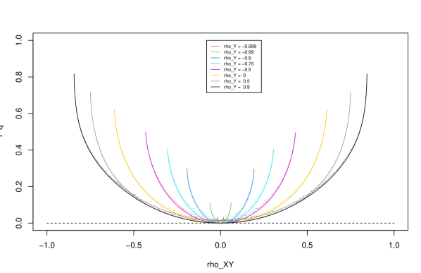
Figure 1: Plots of $T^{q}(\mathbf{Y}|\mathbf{X})$ for $(\mathbf{X},\mathbf{Y})=(X_{1},X_{2},Y_{1},Y_{2})$ being normally distributed (solid lines) and $t$-distributed with $3$ degrees of freedom (dotted) with covariance matrix $\Sigma$ given by (36) in dependence on $\rho_{XY}$ for fixed $\rho_{X}=0.5$ and for several $\rho_{Y}\in\{-0.999,-0.99,-0.9,-0.75,-0.5,0,0.5,0.9\}\,.$

4.2 Continuity results within Fréchet classes

In this section, we study continuity of $T^{q}(\mathbf{Y}|\mathbf{X})$ in Fréchet classes, i.e., in the case where the univariate marginal distributions of $(\mathbf{X},\mathbf{Y})$ are given. Since, in applications, the marginal distributions can often be determined, Fréchet classes play an important role in theory, see, e.g., [18, 28, 47, 64, 71, 76, 88].

For fixed marginal distributions, $T(Y|\mathbf{X})$ depend only on the diagonal of the bivariate distribution function $\psi_{Y|\mathbf{X}}$ in (17). Hence, the following result is an immediate consequence of the dimension reduction principle due to Theorem 2.14.

Proposition 4.8 (Continuity of $T^{q}(\mathbf{Y}|\mathbf{X})$ within Fréchet classes).

Consider the $(p+q)$-dimensional random vector $(\mathbf{X},\mathbf{Y})$ and a sequence $(\mathbf{X}_{n},\mathbf{Y}_{n})_{n\in\mathbb{N}}$ of $(p+q)$-dimensional random vectors such that $X_{i,n}\stackrel{{\scriptstyle\mathrm{d}}}{{=}}X_{i}$ and $Y_{j,n}\stackrel{{\scriptstyle\mathrm{d}}}{{=}}Y_{j}$ for all $i\in\{1,\dots,p\}$, $j\in\{1,\dots,q\}$, and $n\in\mathbb{N}$. If

1. $\psi_{Y_{1,n}|\mathbf{X}_{n}}(t,t)\xrightarrow[n\to\infty]{}\psi_{Y_{1}|\mathbf{X}}(t,t)$ for $P^{Y_{1}}$-almost all $t\,,$

2. $\psi_{Y_{j,n}|(\mathbf{X}_{n},Y_{j-1,n},\dots,Y_{1,n})}(t,t)\xrightarrow[n\to\infty]{}\psi_{Y_{j}|(\mathbf{X},Y_{j-1},\dots,Y_{1})}(t,t)$ for $P^{Y_{j}}$-almost all $t$ for all $j\in\{2,\dots,q\}$

3. $\psi_{Y_{j,n}|(Y_{j-1,n},\dots,Y_{1,n})}(t,t)\xrightarrow[n\to\infty]{}\psi_{Y_{j}|(Y_{j-1},\dots,Y_{1})}(t,t)\,,$ for $P^{Y_{j}}$-almost all $t$ for all $j\in\{2,\dots,q\}$,

then $T^{q}(\mathbf{Y}_{n}|\mathbf{X}_{n})\to T^{q}(\mathbf{Y}|\mathbf{X})\,.$

Remark 4.9.

If $\mathbf{X}$ and $\mathbf{Y}$ have continuous distribution functions, one can resort to the Fréchet class with uniform on $[0,1]$-distributed marginals, i.e., to copulas, because $T^{q}$ satisfies the distributional invariance given by

$$T^{q}(\mathbf{Y}|\mathbf{X})=T^{q}({\bf F}_{\mathbf{Y}}(\mathbf{Y})|{\bf F}_{\mathbf{X}}(\mathbf{X}))$$ (38)

for ${\bf F}_{\mathbf{X}}=(F_{X_{1}},\ldots,F_{X_{p}})$ and ${\bf F}_{\mathbf{Y}}=(F_{Y_{1}},\ldots,F_{Y_{q}})\,,$ see Corollaries 2.5 and 2.6. In other words: In the continuous setting, $T$ and $T^{q}$ are entirely copula-based and margin-free.

As a consequence of Proposition 4.8 and the previous remark, we establish continuity of $T^{q}$ within the class of $l_{1}$-norm symmetric distributions. For the proof of the following result, we make use of continuity properties of Archimedean copulas which are the copulas of $l_{1}$-norm symmetric distributions, see [58]. Denote by $\mathbb{S}_{d}$ a $d$-variate random vector that is uniformly distributed on the unit simplex $\mathcal{S}_{d}=\{x\in\mathbb{R}^{d}\mid\lVert x\rVert_{1}=1\}\,.$ A $d$-variate random vector $\mathbb{W}$ follows an $l_{1}$-norm symmetric distribution if there exists a nonnegative random variable $R$ independent of $\mathbb{S}_{d}$ such that $\mathbb{W}\stackrel{{\scriptstyle\mathrm{d}}}{{=}}R\,\mathbb{S}_{d}\,.$

Proposition 4.10 (Continuity of $T^{q}(\mathbf{Y}|\mathbf{X})$ for $l_{1}$-norm symmetric distributions).

Let $(\mathbf{X}_{n},\mathbf{Y}_{n})\stackrel{{\scriptstyle\mathrm{d}}}{{=}}R_{n}\mathbb{S}_{p+q}$ be a sequence of $l_{1}$-norm symmetric random vectors and let $(\mathbf{X},\mathbf{Y})\stackrel{{\scriptstyle\mathrm{d}}}{{=}}R\,\mathbb{S}_{p+q}\,.$ Assume that $F_{R_{n}}$ and $F_{R}$ are continuous with $F_{R_{n}}(0)=F_{R}(0)=0$ for all $n\in\mathbb{N}\,.$ Then $R_{n}\xrightarrow{~{}d~{}}R$ implies $T^{q}(\mathbf{Y}_{n}|\mathbf{X}_{n})\to T^{q}(\mathbf{Y}|\mathbf{X})\,.$

As an application of Proposition 4.10, it follows that $T$ is continuous w.r.t. the parameters of the bivariate Archimedean copulas in Example 3.8, compare [23]. Extensions to the continuity of $T^{q}$ w.r.t. multivariate Archimedean copulas are immediate.

5 Estimation

In this section, we provide estimators $T_{n}^{q}$ and $\overline{T_{n}^{q}}$ for $T^{q}$ and $\overline{T^{q}}$ defined by (3) and (12), respectively. Both estimators are consistent with the underlying construction principle and based on Azadkia & Chatterjee’s graph-based estimator $T_{n}$ for $T$. The properties of $T_{n}$ imply strong consistency and an asymptotic computation time of $O(n\log n)$ for the estimators $T_{n}^{q}$ and $\overline{T_{n}^{q}}$, respectively. In the second part of this section, asymptotic normality is proved in some specific case. In Subsection 5.3, we give evidence that the proposed estimators perform well in the multivariate normal model where closed-form formulas for $T^{q}(\mathbf{Y}|\mathbf{X})$ are available (see Example 3.10). We refer to Section 6 for applications to real-world data.

5.1 Consistency

In the following, consider a $(p+q)$-dimensional random vector $(\mathbf{X},\mathbf{Y})$ with i.i.d. copies $(\mathbf{X}_{1},\mathbf{Y}_{1})$, $\dots$, $(\mathbf{X}_{n},\mathbf{Y}_{n})$. Recall that $\mathbf{Y}$ is assumed to have non-degenerate components, i.e., for all $i\in\{1,\ldots,q\}\,,$ the distribution of $Y_{i}$ does not follow a one-point distribution.

As an estimator for $T^{q}$ we propose the statistic $T^{q}_{n}$ given by

$$T_{n}^{q} =T_{n}^{q}(\mathbf{Y}|\mathbf{X}):=1-\frac{q-\sum_{i=1}^{q}T_{n}(Y_{i}|(\mathbf{X},Y_{i-1},\dots,Y_{1}))}{q-\sum_{i=1}^{q}T_{n}(Y_{i}|(Y_{i-1},\dots,Y_{1}))}$$ (39)

with $T_{n}$ being the estimator proposed by Azadkia and Chatterjee [4] and given by

$$T_{n}(Y|\mathbf{X}) = \frac{\sum_{k=1}^{n}(n\,\min\{R_{k},R_{N(k)}\}-L_{k}^{2})}{\sum_{k=1}^{n}L_{k}\,(n-L_{k})},$$ (40)

where $R_{k}$ denotes the rank of $Y_{k}$ among $Y_{1},\dots,Y_{n}$, i.e., the number of $j$ such that $Y_{j}\leq Y_{k}$, and $L_{k}$ denotes the number of $j$ such that $Y_{j}\geq Y_{k}$ (see also [40]). For each $k$, the number $N(k)$ denotes the index $j$ such that $\mathbf{X}_{j}$ is the nearest neighbour of $\mathbf{X}_{k}$ with respect to the Euclidean metric on $\mathbb{R}^{p}$. Since there may exist several nearest neighbours of $\mathbf{X}_{k}$ ties are broken at random.
From the definition of $T_{n}$ in (40), it is immediately apparent that the estimator is built on the dimension reduction principle explained in Section 2 (see also [4, Section 11] where the authors prove that $Y_{k}$ and $Y_{N(k)}$ are asymptotically conditionally independent given $\mathbf{X}$), which is key to a fast estimation of $T$ and hence $T^{q}$.

As an estimator for the permutation invariant version $\overline{T^{q}}\,,$ we propose the statistic $\overline{T_{n}^{q}}$ given by

$$\overline{T_{n}^{q}}=\overline{T_{n}^{q}}(\mathbf{Y}|\mathbf{X}):=\frac{1}{q!}\sum_{\sigma\in S_{q}}T_{n}^{q}(\mathbf{Y}_{\sigma}|\mathbf{X})$$ (41)

where $T_{n}^{q}$ is defined by (39).

Azadkia and Chatterjee [4] proved that $T_{n}$ is a strongly consistent estimator for $T$. As a direct consequence, we obtain strong consistency of $T_{n}^{q}$ and $\overline{T_{n}^{q}}$ as follows.

Theorem 5.1 (Consistency).

It holds that $\lim_{n\to\infty}T_{n}^{q}=T^{q}$ almost surely and $\lim_{n\to\infty}\overline{T_{n}^{q}}=\overline{T^{q}}$ almost surely.

Remark 5.2.

1. From the properties of the estimator $T_{n}$, see [4, Remark (1)], it follows that also $T_{n}^{q}$ and $\overline{T_{n}^{q}}$ can be computed in $O(n\log n)$ time, using that the denominator in (3) and (4) takes values only in the interval $[1,q]\,.$

2. The estimators $T_{n}^{q}$ and $\overline{T_{n}^{q}}$ are model-free estimators for $T^{q}$ and $\overline{T^{q}}\,,$ respectively, having no-tuning parameters and being consistent under sparsity assumptions, compare [4].

5.2 Asymptotic normality

The statistic $T_{n}$ and thus the individual terms of the estimator $T_{n}^{q}$ in (39) are proved to behave asymptotically normal, see [55]. However, it is challenging to show asymptotic normality for $T_{n}^{q}$ because $T_{n}(Y_{i}|(\mathbf{X},Y_{i-1},\ldots,Y_{1}))$ and $T_{n}(Y_{i}|(Y_{i-1},\ldots,Y_{1}))$ are generally dependent. For the case where $Y_{1},\ldots,Y_{q}$ are independent and conditionally independent given $\mathbf{X}$ and hence, by Remark 2.8(ii),

$$T^{q}(\mathbf{Y}|\mathbf{X})=T^{\Sigma}(\mathbf{Y}|\mathbf{X})=\frac{1}{q}\sum_{i=1}^{q}T(Y_{i}|\mathbf{X})$$

we make use of the results in [55] in order to prove asymptotic normality for

$$T_{n}^{\Sigma}=T_{n}^{\Sigma}(\mathbf{Y}|\mathbf{X}):=\frac{1}{q}\sum_{i=1}^{q}T_{n}(Y_{i}|\mathbf{X})\,,$$

which serves as estimator for $T^{\Sigma}$, as follows.

Proposition 5.3 (Asymptotic normality for special case).

Assume that

1. the distribution function of $(\mathbf{X},\mathbf{Y})$ is continuous,

2. $\mathbf{Y}$ is not a measurable function of $\mathbf{X}$, and

3. $Y_{1},\ldots,Y_{q}$ are independent and conditionally independent given $\mathbf{X}$.

Then

$$\lim_{n\to\infty}\frac{T_{n}^{\Sigma}-\mathbb{E}[T_{n}^{\Sigma}]}{\mathrm{Var}(T_{n}^{\Sigma})}\stackrel{{\scriptstyle d}}{{=}}N(0,1).$$

Remark 5.4.

1. For $q=1\,,$ Proposition 5.3 simplifies to [55, Theorem 1.1] which provides asymptotic normality of $T_{n}^{\Sigma}$ under general assumptions. For $q>1$ endogenous variables and under additional assumptions on the dependence structure of $\mathbf{Y}$ under which $T^{q}(\mathbf{Y}|\mathbf{X})=\overline{T^{q}}(\mathbf{Y}|\mathbf{X})=T^{\Sigma}(\mathbf{Y}|\mathbf{X})$ (see Remark 2.8(ii)), Proposition 5.3 proves asymptotic normality of $T_{n}^{\Sigma}$ as estimator for $T^{\Sigma}$ and hence as estimator for $T^{q}$ and $\overline{T^{q}}\,.$ While conditional independence is a standard assumption for several statistical models, see, e.g., [20], independence of $Y_{1},\ldots,Y_{q}$ ensures that $T(Y_{i}|(Y_{i-1},\ldots,Y_{1}))=0$ for all $i\in\{1,\dots,q\}\,.$

2. If $\mathbf{Y}$ is assumed to be perfectly dependent in the sense that $Y_{i}=f_{i}(Y_{1})$ for all $i\in\{2,\ldots,q\}\,,$ then $T^{q}(\mathbf{Y}|\mathbf{X})$ simplifies to $T(Y_{1}|\mathbf{X})\,,$ see Remark 2.8(iii). In this case, $T_{n}(Y_{1}|\mathbf{X})$ serves as an asymptotically normal estimator for $T(Y_{1}|\mathbf{X})$ and hence for $T^{q}(\mathbf{Y}|\mathbf{X})$.

5.3 Simulation study in multivariate normal models

We illustrate the small and moderate sample performance of our estimator $T_{n}^{q}$ in the case the random vector $(\mathbf{X},\mathbf{Y})$ follows a multivariate normal distribution according to Example 3.10 with

1. $p=5$ exogenous and $q=2$ endogenous variables and correlation parameters $\rho_{X}=0.5$, $\rho_{Y}=0.2$, $\rho_{XY}=0.5$, and

2. $p=2$ exogenous and $q=4$ endogenous variables and correlation parameters $\rho_{X}=0.25$, $\rho_{Y}=0.75$, $\rho_{XY}=0.5$,

respectively. To test the performance of the estimator $T_{n}^{q}$ in different settings, samples of size $n\in\{20;50;100;200;500;1,000;5,000;10,000;50,000\}$ are generated and then $T_{n}^{q}$ is calculated. These steps are repeated $R=1,000$ times. Fig. 2 depicts the estimates of $T_{n}^{q}$ for different samples sizes and relates it to the true dependence value (dashed red line).

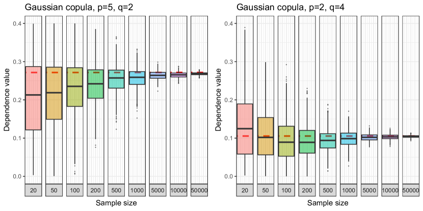
Figure 2: Boxplots summarizing the $1,000$ obtained estimates for $T_{n}^{q}$. Samples of size $n$ are drawn from a multivariate normal distribution with $5$ exogenous and $2$ endogenous variables (left panel) and with $2$ exogenous and $4$ endogenous variables (right panel).

As can be observed from Figure 2 (and as expected), the estimates converge rather fast to the true values. Notice that the estimator $\overline{T^{q}_{n}}$ performs comparably to $T_{n}^{q}$, which is not surprising given the exchangeability of the endogenous variables in the normal models considered.

6 Applications

In this section, we illustrate the capability and importance of our extensions $T^{q}$ in (3) and $\overline{T^{q}}$ in (12) of Azadkia & Chatterjee’s rank correlation. The introduced extensions not only allow for a model-free and dependence-based feature ranking and forward feature selection of multi-outcome data, but also enable the identification of networks between an arbitrary number of random variables based on the degree of predictability among them.

In the first part of this section, a model-free and dependence-based feature ranking and forward feature selection method for multi-outcome data called MFOCI (multivariate feature ordering by conditional independence) is introduced that is proven to be consistent (Subsection 6.1). We illustrate that MFOCI is plausible in the sense that it chooses a small number of variables that include, in particular, the most important variables for the individual feature selections, analyzing climate data as well as medical data as examples. In Subsection 6.1.2, MFOCI is compared with other feature selection methods for multi-output data discussed in the literature, with the result that MFOCI achieves similar prediction errors than other methods but with a (considerably) smaller number of selected variables, resulting in a significant reduction in complexity. Finally, Subsection 6.2 contains an application of $T^{q}$ to finance and illustrates the identification of networks between banks also via a hierarchical cluster analysis for random variables, as discussed in [36].

6.1 Feature Selection

In the literature, numerous variable selection methods for a single output variable $Y$ (i.e., $q=1$) are studied. Model-dependent methods are mostly based on linear or additive models, see, e.g., [10, 29, 30, 33, 38, 60, 66, 90, 91] and [12, 19, 43, 86] for overviews; model-free methods rely on random forests ([7, 8]), mutual information ([5, 87]), or measures of predictability ([4, 44]). However, up to our knowledge, there is rather little literature on feature selection methods that are applicable to multivariate endogenous variables (i.e., for $q>1$). In the class of linear methods, the lasso allows an extension to multiple output data ([82][83]), while the kernel feature ordering by conditional independence in [44] is a general model-free method defined for reproducing kernel Hilbert spaces.

Since the measures of predictability $T^{q}$ and $\overline{T^{q}}$ satisfy the information gain inequality and characterize conditional independence between multivariate random vectors (see Theorem 2.2 and Corollary 2.7), they are suitable for a new subset selection method for predicting multivariate variables. We adapt to [4, Chapter 5] and extend their feature selection method called FOCI (feature ordering by conditional independence) from $q=1$ to arbitrary output dimension $q\in\mathbb{N}$ which we denote MFOCI (multivariate feature ordering by conditional independence) and works as follows:
For the vector $\mathbf{Y}=(Y_{1},\dots,Y_{q})$ of $q\geq 1$ endogenous variables and the vector $\mathbf{X}=(X_{1},\dots,X_{p})$ of $p\geq 1$ exogenous variables, consider i.i.d. copies $(\mathbf{X}_{1},\mathbf{Y}_{1}),\dots,(\mathbf{X}_{n},\mathbf{Y}_{n})$ of $(\mathbf{X},\mathbf{Y})$. First, denote by $j_{1}$ the index $j$ maximizing $T^{q}_{n}(\mathbf{Y}|X_{j})$. Now, assume that after $k$ steps MFOCI has chosen variables $X_{j_{1}},\dots,X_{j_{k}}$ and denote by $j_{k+1}$ the index $j\in\{1,\dots,p\}\backslash\{j_{1},\dots,j_{k}\}$ maximizing $T^{q}_{n}(\mathbf{Y}|(X_{j_{1}},\dots,X_{j_{k}},X_{j}))$. The algorithm stops with the first index $k$ for which $T^{q}_{n}(\mathbf{Y}|(X_{j_{1}},\dots,X_{j_{k}},X_{j_{k+1}}))\leq T^{q}_{n}(\mathbf{Y}|(X_{j_{1}},\dots,X_{j_{k}}))$, i.e., with the first index for which the degree of predictability no longer increases when adding further explanatory variables. Finally, denote by $\hat{S}:=\{j_{1},\dots,j_{k}\}$ the subset selected by the above algorithm. In case the stopping criterion is not fulfilled for any $k$ we set $\hat{S}:=\{1,\dots,p\}$. In case $T^{q}_{n}(\mathbf{Y}|X_{j_{1}})\leq 0$ the set $\hat{S}$ is chosen to be empty.

A subset $S\subseteq\{1,\ldots,p\}\,,$ is called sufficient if $\mathbf{Y}$ and $\mathbf{X}_{S}:=(X_{j})_{j\in S}$ are conditionally independent given $\mathbf{X}_{S^{c}}:=(X_{j})_{j\in S^{c}}\,,$ where $S^{c}:=\{1,\ldots,p\}\setminus S\,.$ By adapting to [4, Chapter 6], we now discuss consistency of MFOCI for the case when, for every $i\in\{1,\dots,q\}$, there exist $\delta^{i}>0$ such that for any insufficient subset $S$ there is some $j\notin S$ with

$$\int_{\mathbb{R}}{\rm var}(P(Y_{i}\geq y\,|\,(\mathbf{X}_{S\cup\{j\}},Y_{i-1},\dots,Y_{1})))\;\mathrm{d}P^{Y_{i}}(y)$$ (42)

$$\geq \int_{\mathbb{R}}{\rm var}(P(Y_{i}\geq y\,|\,(\mathbf{X}_{S},Y_{i-1},\dots,Y_{1})))\;\mathrm{d}P^{Y_{i}}(y)+\delta^{i}$$

The following weak assumptions comprise a local Lipschitz condition for the conditional distributions and an exponential boundedness condition for tail probabilities, respectively, see [4, Chapter 4 and Proposition 4.2] for a detailed discussion of the assumptions.

Assumption 6.1.

For all $i\in\{1,\ldots,q\}\,,$ there exist real numbers $\beta^{i},C^{i}\geq 0$ such that for any subset $S\subseteq\{1,\ldots,p\}$ with $|S|\leq 1/\delta^{i}+2\,,$ any $\mathbb{x},\mathbb{x}^{\prime}\in\mathbb{R}^{|S|}\,,$ any $\mathbb{y}\in\mathbb{R}^{i-1}\,,$ and any $t\in\mathbb{R}\,,$

$$|P(Y_{i}\geq t\mid\mathbf{X}_{S}=\mathbb{x},(Y_{i-1},\ldots,Y_{1})=\mathbb{y})-P(Y_{i}\geq t\mid\mathbf{X}_{S}=\mathbb{x}^{\prime},(Y_{i-1},\ldots,Y_{1})=\mathbb{y})|$$

$$\leq C^{i}\left(1+\lVert(\mathbb{x},\mathbb{y})\rVert^{\beta^{i}}+\lVert(\mathbb{x}^{\prime},\mathbb{y})\rVert^{\beta^{i}}\right)\lVert\mathbb{x}-\mathbb{x}^{\prime}\rVert\,.$$

Assumption 6.2.

For all $i\in\{1,\ldots,q\}\,,$ there exist $C_{1}^{i},C_{2}^{i}>0$ such that for any subset $S\subseteq\{1,\ldots,p\}$ with $|S|\leq 1/\delta^{i}+2$ and for any $t>0\,,$ $P(\lVert(\mathbf{X}_{S},Y_{i-1},\dots,Y_{1})\rVert\geq t)\leq C_{1}^{i}e^{-C_{2}^{i}t}\,.$

As an immediate consequence of [4, Theorem 6.1] and the inequality

$$P\left(\cap_{i=1}^{q}E_{i}\right) \geq\max\left\{\sum_{i=1}^{q}P(E_{i})-(q-1),0\right\}$$

for events $E_{1},\dots,E_{q}$, the following result states that the subset of selected explanatory variables via MFOCI is sufficient with high probability.

Proposition 6.3 (Consistency).

Suppose that $\delta^{1},\ldots,\delta^{q}>0$ and that Assumptions 6.1 and 6.2 are satisfied. Let $\hat{S}$ be the subset selected by MFOCI with a sample size of $n\,.$ Then, for all $i\in\{1,\ldots,q\}\,,$ there exist $L_{1}^{i},L_{2}^{i},L_{3}^{i}>0$ depending only on $C^{i},\beta^{i},C_{1}^{i},C_{2}^{i}$ and $\delta^{i}$ such that

$$P(\hat{S}\text{ is sufficient})\geq 1-\sum_{i=1}^{q}L_{1}^{i}(p+i-1)^{L_{2}^{i}}e^{-L_{3}^{i}n}\,.$$ (43)

In the sequel, we use real-world data to demonstrate the relevance of $T^{q}$ and $\overline{T^{q}}$ in forward feature selection extracting the most important variables for predicting a vector $\mathbf{Y}$ of endogenous variables.

6.1.1 Plausibility of multivariate feature selection

Exemplarily we evaluate bioclimatic data as well as medical data to illustrate that MFOCI is plausible in the sense that it chooses a small number of variables that include, in particular, the most important variables for the individual feature selections.

Analysis of global climate data: We first consider a data set of bioclimatic variables for $n=1862$ locations homogeneously distributed over the global landmass from CHELSEA ([48, 49]) and analyze the influence of a set of thermal and precipitation-related variables (see Table 1) on Annual Mean Temperature (AMT) and Annual Precipitation (AP). By applying the coefficient $T^{q}$ we first perform a hierarchical feature selection and identify those variables that best predict the endogenous vector (AMT,AP) (= variables $(Y_{1},Y_{2})$). Then, we compare the outcome with the hierarchical feature selections that refer to the individual endogenous variables. First, notice that the Pearson correlation between the endogenous variables AMT and AP is $0.52$, their Spearman’s rank correlation equals $0.61$.

Table 1: Thermal and precipitation-related variables used as exogenous variables; see Subsection 6.1.1 for details.

MTWeQ	Mean Temperature of Wettest Quarter
MTDQ	Mean Temperature of Driest Quarter
MTWaQ	Mean Temperature of Warmest Quarter
MTCQ	Mean Temperature of Coldest Quarter
PTWeQ	Precipitation of Wettest Quarter
PTDQ	Precipitation of Driest Quarter
PTWaQ	Precipitation of Warmest Quarter
PTCQ	Precipitation of Coldest Quarter

Table 2 depicts the order of the via MFOCI selected variables based on the estimated values for $T^{q}$. There, the values in line $k$ indicate the estimated values for $T^{q}(\mathbf{Y}|(X_{1},\dots,X_{k}))$ where $X_{1},\dots,X_{k}$ are the variables in lines $1$ to $k$. For the prediction of the exogenous vector $(Y_{1},Y_{2})=$ (AMT, AP), MFOCI selects the four variables {MTWaQ, PWeQ, MTCQ, PDQ} (at this point it is worth mentioning that both the feature selection referring to the permuted vector $(Y_{2},Y_{1})=$ (AP, AMT) and the feature selection based on $\overline{T^{q}}$ identify the same four relevant variables.). For the prediction of the exogenous variable AMT and AP, respectively, MFOCI selects the variables {MTWaQ, MTCQ, MTWeQ} and {PWeQ, PDQ, PCQ}, respectively. Remarkably, from this perspective, the chosen explanatory variables of the multivariate feature selection for $(Y_{1},Y_{2})=$ (AMT,AP) are a proper subset of the union of the relevant explanatory variables of the respective individual feature selections.

Table 2: Results of the hierarchical feature selections based on the coefficients $T$ and $T^{2}$, respectively, to identify those variables that best predict AMT and AP and (AMT,AP), respectively; see Subsection 6.1.1 for details. The variables selected via MFOCI to predict (AMT,AP) are marked in red color.

Position	Variables to predict (AMT,AP)	$T^{2}_{n}$	Variables to predict AMT	$T_{n}$	Variables to predict AP	$T_{n}$
1	MTWaQ	0.64	MTWaQ	0.84	PWeQ	0.80
2	PWeQ	0.84	MTCQ	0.97	PDQ	0.92
3	MTCQ	0.89	MTWeQ	0.98	PCQ	0.93
4	PDQ	0.91

We observe from Table 2 that $T^{q}$ might fulfill some kind of reversed information gain inequality in the endogenous part, i.e., adding endogenous variables might lower predictability. In general, however, such behaviour cannot be inferred, see Example 2.9, where $T^{q}((Y_{1},Y_{2})|X)=1/4>0=\max\{T^{q}(Y_{1}|X),T^{q}(Y_{2}|X)\}$.

Predicting the extent of Parkinson’s disease: As illustrative example for feature selection in medicine, we determine the most important variables for predicting two UPDRS scores–the motor as well as the total UPDRS score–which are assessment tools used to evaluate the extent of Parkinson’s disease in patients. The data set consists of $n=5875$ observations including the two predicting variables (motor and total UPDRS score) as well as the exogenous variables age, sex, and several data concerning shimmer and jitter which are related to the voice of the patient. While shimmer measures fluctuations in amplitude, jitter indicates fluctuations in pitch. Common symptoms of Parkinson’s disease include speaking softly and difficulty maintaining pitch. Therefore, measurements of both shimmer and jitter can be used to detect Parkinson’s disease and thus the voice data can be useful for predicting the UPDRS scores. Note that the predicting variables Motor UPDRS score and Total UPDRS score are strongly dependent–the data yield Spearman’s correlation of $0.95$ and Kendall’s correlation of $0.85\,.$

Table 3: Results of the hierarchical feature selections based on the coefficients $T$ and $T^{2}$, respectively, to identify those variables that best predict Motor UPDRS score, Total UPDRS score, as well as both Motor UPDRS score and Total UPDRS score, respectively; see Subsection 6.1.1 for details. The variables selected via MFOCI to predict (Motor UPDRS score,Total UPDRS score) are marked in red color.

Position	Variables to predict Motor and Total UPDRS score	$T^{2}_{n}$	Variables to predict Motor UPDRS score	$T_{n}$	Variables to predict Total UPDRS score	$T_{n}$
1	age	0.5316	age	0.4935	age	0.5154
2	sex	0.6759	sex	0.6604	sex	0.6711
3	DFA	0.7433	DFA	0.7383	DFA	0.7413
4	Shimmer.APQ11	0.7668	RPDE	0.7581	RPDE	0.7668
5	RPDE	0.7707	Shimmer.dB	0.7651	Shimmer.dB	0.7745
6	Shimmer.DDA	0.7783	Shimmer.DDA	0.7693	Shimmer.DDA	0.7760
7	NHR	0.7801	Shimmer.APQ5	0.7696	Shimmer.APQ5	0.7780
8	Shimmer	0.7822	Shimmer.APQ11	0.7703	Jitter.RAP	0.7781
9	Shimmer.APQ5	0.7834
10	Jitter.Abs.	0.7838
11	Jitter.RAP	0.7840

From Table 3, we observe that MFOCI selects 11 variables for predicting both UPDRS scores of Parkinson patients jointly, while 8 variables are selected for predicting each score individually. The most important variables for jointly and individually predicting the UPDRS scores of Parkinson patients are age, sex, and DFA (the signal fractal scaling exponent), making MFOCI plausible in this case as well. The order of the seven most important variables are the same when predicting the individual scores. However, our feature selection recommends a different order from the fourth position on when predicting the scores jointly. Interestingly, from the fourth or fifth variable on, the value of $T_{n}^{2}$ resp. $T_{n}$ increases only slightly. Since $T^{q}$ and $T$ characterize conditional independence, and a small increase is associated with only slightly greater squared variability of the conditional distribution functions, one could argue that in all cases a total of 4 or 5 of the 18 characteristics are sufficient to predict one or both of the variables. If we compare the values $T_{n}$ and $T_{n}^{2}\,,$ we find that they are very similar which can be explained by the strong positive dependence of the individual scores.

6.1.2 Multivariate feature selection comparison

We compare the hierarchical feature selection method MFOCI based on our extensions of Azadkia & Chatterjee’s rank correlation $T^{q}$ and $\overline{T^{q}}$ with other methods including (1) the kernel feature ordering by conditional independence (KFOCI, in short) introduced by Huang, Deb and Sen [44], (2) the Lasso (see Tibshirani [82, 83]), and (3) the bivariate vine copula based quantile regression (BVCQR, in short) proposed by Tepegjozova and Czado [81, Section 6].

We first revisit the global climate data set in Subsection 6.1.1 and compare the feature selection outcome obtained via MFOCI (see Table 2) with KFOCI and Lasso. Due to Table 4, the procedure via Lasso ends with 7 explanatory variables, the procedure via KFOCI (where we apply the kernel rbfdot(1)) ends with 5 explanatory variables, and both MFOCI via $T^{q}$ and KFOCI applying the default kernel end with the same 4 explanatory variables (even though the order differs). Note that KFOCI is used here with default number of nearest neighbours. For each subset of selected variables, the (cross validated) mean squared prediction error (MSPE) based on a random forest are calculated using R-package MultivariateRandomForest.

Table 4: Chosen explanatory variables to predict (AMT, AP) selected via MFOCI, KFOCI and Lasso with MSPEs for each response variable; see Subsection 6.1.2 for details. The variables selected via MFOCI to predict (AMT,AP) are marked in red color.

Variables to predict (AMT, AP)	Feature selection via MFOCI	Feature selection via KFOCI, default kernel	Feature selection via KFOCI, kernel rbfdot(1)	Feature selection via Lasso
	MTWaQ		MTWaQ	PDQ
	PWeQ		PWeQ	PWeQ
	MTCQ		PCQ	PCQ
	PDQ		PWaQ	PWaQ
			PDQ	MTCQ
				MTWaQ
				MTWeQ
MSPE for response AMT	158		633	151
MSPE for response AP	14352		14529	13467

In a second step we compare our method MFOCI based on $\overline{T^{q}}$ also with BVCQR, another dependence-based method proposed in [81]. The underlying data consist of the Seoul weather data set containing daily observations of two endogenous variables, NextMin: daily minimum air temperature for the next day and NextMax: daily maximum air temperature for the next day, and 13 explanatory variables from June 30 to August 30 during 2013-2017 of weather station central Seoul (sample size $n=307$). All the variables in this data set exhibit quite high dependencies; for instance, the Pearson correlation between the endogenous variables NextMin and NextMax is $0.65$.
In order to achieve comparability with the feature ranking computed in [81], we are compelled to ignore for the moment the temporal dependence between daily measurements. Then the feature selection procedure via BVCQR ends with 11 explanatory variables, KFOCI (kernel rbfdot(1) & default kernel, both with default number of nearest neighbours) ends with 6 explanatory variables, Lasso ends with 5 explanatory variables, while MFOCI via $\overline{T^{q}}$ and KFOCI (kernel rbfdot(1) with number of nearest neighbours = 1) end with (different) subsets of no more than 4 variables. For each subset of selected variables we calculate the (cross validated) mean squared prediction error (MSPE) based on a random forest using R-package MultivariateRandomForest. Table 5 depicts the subsets of chosen explanatory variables and lists the MSPEs for each response.

To conclude, MFOCI achieves similar prediction errors as the other methods, but with a considerably smaller number of selected variables than Lasso and BVCQR resulting in a significant reduction in complexity. MFOCI and KFOCI perform comparably well, however, the variable selection via KFOCI exhibits a sensitivity to the kernel used.

Table 5: Chosen explanatory variables to predict (NextMax, NextMin) selected via MFOCI, BVCQR, KFOCI and Lasso with MSPEs for each response variable; see Subsection 6.1.2 for details. The variables selected via MFOCI to predict (NextMax, NextMin) are marked in red color.

Variables to predict (NextMax, NextMin)	Feature selection via MFOCI	Feature selection via BVCQR	Feature selection via KFOCI, kernel rbfdot(1) & default kernel	Feature selection via KFOCI, kernel rbfdot(1) (Knn = 1)	Feature selection via Lasso
	LDAPS_Tmin	LDAPS_Tmin	LDAPS_Tmin	LDAPS_Tmin	LDAPS_Tmax
	LDAPS_Tmax	LDAPS_Tmax	LDAPS_Tmax	LDAPS_Tmax	LDAPS_Tmin
	LDAPS_CC3	LDAPS_RHmax	LDAPS_CC1	LDAPS_RHmin	LDAPS_CC1
	LDAPS_CC1	LDAPS_WS	LDAPS_CC2	LDAPS_CC2	LDAPS_CC2
		Present_Tmin	LDAPS_CC4		Present_Tmax
		LDAPS_CC1	LDAPS_CC3
		Present_Tmax
		LDAPS_LH
		LDAPS_CC3
		LDAPS_RHmin
		LDAPS_CC4
MSPE NextMax	2.55	2.40	2.57	2.81	2.63
MSPE NextMin	1.09	1.07	1.03	1.05	1.03

6.2 Identifying networks

Since $T^{q}$ is able to measure the strength of (directed) dependence between random vectors of different dimensions, there are plenty of ways to identify and visualize networks of dependencies. As examples from finance, we analyze and illustrate the interconnectedness of banks (Section 6.2.1) and consider a clustering method for random variables based on the measure $T^{q}$ (Section 6.2.2), see [24, 54, 36] for similar methods based on dissimilarity measures. Note that recently developed methods for clustering random variables differ from the well-studied clustering of data, see, e.g., [27, 37] for an overview of cluster analyses of data.

6.2.1 Interconnectedness

We consider the interconnectedness of the $3$ largest banks in each of the U.S. (US), Europe (EU) and Asia and Pacific (AP), and compare further their connectedness with the $4$th largest banks in the US and Europe, which are the Citigroup (CG) and Deutsche Bank (DB), respectively. The three largest banks of the U.S. comprise JP Morgan (JPM), Bank of America (BAC), and Wells Fargo (WFC). The three largest banks of Europe comprise HSBC, BNP Paribas (BNP), and Crédit Agricole (CAG), and the three largest banks of Asia and Pacific comprise the Industrial and Commercial Bank of China (ICBC), the China Construction Bank Corporation (CCB), and the Agricultural Bank of China (ABC).

For revealing the interconnectedness of the banks, we estimate their predictability via $T^{q}$ from a sample of daily log-returns of the Banks’ stock data (in USD) over a time period from April 7, 2011 to December 14, 2022. We assume that the log-returns are i.i.d., which is a standard assumption for stock data, see, e.g., [57]. Figure 3 shows the values of $T_{n}^{q}$ for the above described interrelations. We oberserve that

• The three largest U.S. banks have a greater influence on the other banks than vice versa.

• There is little dependence of the largest U.S. and European banks on the largest Asian banks.

• The dependence of the fourth largest U.S. bank (CG) on the three largest U.S. banks is relatively large. Similarly, the fourth-largest European bank is quite dependent on the three largest European banks. Further, dependence of individual banks on Asian banks should not be neglected.

We mention that there is high pairwise correlation between the log-returns of the largest U.S., the largest European, and the largest Asian banks, respectively. For example, Spearman’s rank correlation of log-returns among the largest U.S. banks ranges from 0.76 to 0.85. Recall that our proposed rank-based measure $T^{q}$ can also measure the influence between multiple input and output variables.

6.2.2 Clustering

As another application of the measure $T^{q}\,,$ we perform a cluster analysis, using the bank data from Section 6.2.1. Our aim is to appropriately partition the set $\mathcal{X}=\{X_{1},\ldots,X_{m}\}$ of the $3$ largest banks in the US (US), Europe (EU) and Asia and Pacific (AP), i.e., $m=9$, into non-empty and non-overlapping classes. To this end, we employ the hierarchical clustering procedure proposed in [36, Section 4], where the different steps of the agglomerative hierarchical clustering algorithm based on a suitable dissimilarity measure $d$ are as follows (any subset of $\mathcal{X}$ will be denoted by upper-case black-board letters):

1. Each object of $\mathcal{X}$ forms a class.

2. For each pair of classes $\mathbb{X}_{1}$ and $\mathbb{X}_{2}$, one computes its dissimilarity degree $d(\mathbb{X}_{1},\mathbb{X}_{2})$.

3. A pair of classes having the smallest dissimilarity degree, say $\{\mathbb{X}_{1},\mathbb{X}_{2}\}$, is identified, then the composite class $\mathbb{X}_{1}\cup\mathbb{X}_{2}$ is formed and the number of classes is decremented.

4. Steps (2), (3) and (4) are repeated until the number of classes is equal to 1.

As dissimilarity measure $d$ we here propose the distance to $1$ (which corresponds to perfect dependence) of the maximum predictability between two given disjoint subsets $\mathbb{X}_{1}=\{X_{11},\dots,X_{1j}\}$ and $\mathbb{X}_{2}=\{X_{21},\dots,X_{2k}\}$ of the random quantities $\{X_{1},\ldots,X_{m}\}$, i.e.,

$$d(\mathbb{X}_{1},\mathbb{X}_{2})$$

$$:=1-\max\left\{T^{|\mathbb{X}_{1}|}\big{(}(X_{11},\dots,X_{1j})\big{|}(X_{21},\dots,X_{2k})\big{)},T^{|\mathbb{X}_{2}|}\big{(}(X_{21},\dots,X_{2k})\big{|}(X_{11},\dots,X_{1j})\big{)}\right\}.$$

Figure 4 illustrates in a dendrogram the clustering output based on the log-return data of the three largest US, EU and AP banks. We oberserve that

• The three largest U.S. banks are highly interconnected.

• The two French banks BNP and CAG are highly interconnected, while the British bank HSBC is more interlinked with the US market.

• The interconnectedness between AP banks is less pronounced.

Figure 3: Interconnectedness of the three largest banks in the US, Europe and Asia and Pacific, as well as connectedness with the banks Citigroup and Deutsche Bank measured by $T^{q}\,;$ see Subsection 6.2.2 for details.

Figure 4: Clustering of the three largest banks in the US, Europe and Asia and Pacific measured by $T^{q}\,;$ see Subsection 6.2.2 for details.

7 A new class of measures of predictability generated by $\leq_{S}$

As demonstrated in detail in Theorem 3.5, the Schur order for conditional distributions $\leq_{S}$ turns out to be a natural ordering of predictability, as it not only proves to be consistent with the measure $T$ defined by (1), but also comprises the axioms of a measure of predictability, the information gain inequality, the characterization of conditional independence, the data processing inequality and self-equitability at the level of orderings (see Theorem 3.5). The Schur order further allows a dimension reduction (see Lemma 3.3) which we employ in the first part of this section to construct new measures of predictability for $\mathbf{Y}$ given $\mathbf{X}$ by evaluating bivariate CIS random vectors (Subsection 7.1). In the second part, we emphasize the specificity of $T^{q}$ as a member of the novel class of measures of predictability.

7.1 A general construction principle

For the construction of a new class of measures of predictability, the basic idea is to use the fundamental properties of the Schur order for conditional distributions as given in Theorem 3.5. Due to the dimension reduction principle in Lemma 3.3, it is sufficient to consider bivariate CIS distributions for analyzing the extent of predictability in the sense of the Schur order for conditional distributions.

First, denote for univariate distribution functions $F_{1}$ and $F_{2}$ by

$$\mathcal{F}(F_{1},F_{2}):=\left\{F\colon\mathbb{R}^{2}\to[0,1]\mid F\text{ is cdf with }F(x,\infty)=F_{1}(x)\,,F(\infty,x)=F_{2}(x)\text{ f.a. }x\in\mathbb{R}\right\}$$

the Fréchet class of all bivariate distribution functions with marginal distribution functions $F_{1}$ and $F_{2}\,,$ respectively. Now, let $\mathcal{F}^{\prime}\subseteq\mathcal{F}(F_{1},F_{2})$ be a Fréchet subclass with $\Pi^{2}\circ(F_{1},F_{2})\in\mathcal{F}^{\prime}$ and $M^{2}\circ(F_{1},F_{2})\in\mathcal{F}^{\prime}\,,$ where $\Pi^{2}(u,v):=uv$ and $M^{2}(u,v):=\min\{u,v\}\,,$ $u,v\in[0,1]\,,$ denote the independence copula and the upper Fréchet copula, respectively. Then a functional $K$ on $\mathcal{F}^{\prime}$ is said to be normalized and strictly $\leq_{lo}$-increasing if

$$K(\Pi^{2}\circ(F_{1},F_{2}))=0\,,~{}~{}~{}K(M^{2}\circ(F_{1},F_{2}))=1\,,~{}$$ (44)

and $$K(F)<K(G)~{}~{}~{}\text{whenever }F\leq_{lo}G\text{ for }F,G\in\mathcal{F}^{\prime}(F_{1},F_{2})\text{ with }F\neq G\,.$$ (45)

We also write $K(W,Y):=K(F)$ for a bivariate random vector $(W,Y)$ with distribution function $F\in\mathcal{F}^{\prime}\,.$

In the sequel, we construct a new class of measures of predictability based on the bivariate CIS transformations in Lemma 3.3. Therefore, consider the Fréchet subclass

$$\mathcal{F}_{\text{\rm\tiny CIS}}(F_{1},F_{2}):=\{F\in\mathcal{F}(F_{1},F_{2})\mid\exists\,(W,Y) \text{ such that }F_{W,Y}=F,~{}(W,Y)\text{ is CIS}\}$$

of distribution functions of bivariate CIS random vectors (see (26) for the definition of CIS). Due to the following lemma, a normalized and strictly $\leq_{lo}$-increasing functional $K$ defined on a Fréchet class of bivariate CIS distributions satisfies the axioms of a measure of predictability.

Lemma 7.1.

Let $K$ be a normalized and strictly $\leq_{lo}$-increasing functional on $\mathcal{F}_{\text{\rm\tiny CIS}}(F_{1},F_{2})\,.$ Then it holds that

1. $K(F)\in[0,1]\,,$

2. $K(F)=0$ if and only if $F(x,y)=F_{1}(x)F_{2}(y)$ for all $x,y\in\mathbb{R}\,,$

3. $K(F)=1$ if and only if $F(x,y)=\min\{F_{1}(x),F_{2}(y)\}$ for all $x,y\in\mathbb{R}\,.$

Several functionals $K$ on $\mathcal{F}_{\text{\rm\tiny CIS}}(F_{1},F_{2})$ satisfying (44) and (45) are given in Example 7.3 below.

Now, applying the dimension reduction principle from Lemma 3.3, we transform the conditional distributions of $Y_{i}|(\mathbf{X},Y_{i-1},\ldots,Y_{1})$ and $Y_{i}|(Y_{i-1},\ldots,Y_{1})$ to bivariate CIS distributions. Therefore, let $U_{i},U_{i}^{\prime},V_{i},V_{i}^{\prime}\sim U(0,1)\,,$ $i\in\{1,\ldots,q\}\,,$ be i.i.d. random variables. Then, define for the ($p+q$)-dimensional random vector $(\mathbf{X},\mathbf{Y})$ the bivariate CIS random vectors

$$(U_{i},Y_{i}^{\prime}) :=(U_{i},q^{\uparrow U_{i}}_{Y_{i}|(\mathbf{X},Y_{i-1},\ldots,Y_{1})}(U_{i}^{\prime}))~{}~{}~{}\text{and}$$ (46)

$$(V_{i},Y_{i}^{\prime\prime}) :=(V_{i},q^{\uparrow V_{i}}_{Y_{i}|(Y_{i-1},\ldots,Y_{1})}(V_{i}^{\prime}))~{}~{}~{}\text{for }i\in\{1,\ldots,q\}\,,$$ (47)

which depend on the rearranged quantile transforms defined by (25). Recall that these bivariate random vectors comprise the extent of predictability of $\mathbf{Y}$ given $\mathbf{X}$ (in the sense of the Schur order) due to Proposition 3.4 and Theorem 3.5 (ii) to (v). Note that $V_{1}$ and $Y_{1}^{\prime\prime}$ are independent by definition of $Y_{1}^{\prime\prime}\,.$

Similar to the shape of $T^{q}$ in (3), define the functional $K^{q}(\mathbf{Y}|\mathbf{X})$ by

$$K^{q}(\mathbf{Y}|\mathbf{X}) :=\frac{\sum_{i=1}^{q}\left[K_{i}(U_{i},Y_{i}^{\prime})-K_{i}(V_{i},Y_{i}^{\prime\prime})\right]}{\sum_{i=1}^{q}\left[1-K_{i}(V_{i},Y_{i}^{\prime\prime})\right]}=1-\frac{q-\sum_{i=1}^{q}K_{i}(U_{i},Y_{i}^{\prime})}{q-\sum_{i=1}^{q}K_{i}(V_{i},Y_{i}^{\prime\prime})}\,.$$ (48)

Due to the dimension reduction principle in Lemma 3.3(iii), the relevant dependence information (in the sense of $\leq_{S}$) of $\mathbf{Y}$ from $\mathbf{X}$ is included in the bivariate random vectors $\{(U_{i},Y_{i}^{\prime}),(V_{i},Y_{i}^{\prime\prime})\}_{i\in\{1,\dots,q\}}$ which all are independent by construction. Consequently, $K^{q}(\mathbf{Y}|\mathbf{X})$ is a combination of $2q$ independent terms. In contrast to that, in $T^{q}(\mathbf{Y}|\mathbf{X})$ defined by (3) the random vector $(\mathbf{X},\mathbf{Y})$ enters directly and the individual $2q$ terms are generally dependent.

The following result gives sufficient conditions on $K_{1},\ldots,K_{q}$ such that $K^{q}(\mathbf{Y}|\mathbf{X})$ is a measure of predictability. Denote by $F_{U(0,1)}$ the distribution function of the uniform distribution on $(0,1)\,.$

Theorem 7.2 (Fundamental properties of $K^{q}$).

For all $i\in\{1,\ldots,q\}\,,$ let $K_{i}$ be a normalized and strictly $\leq_{lo}$-increasing functional on $\mathcal{F}_{\text{\rm\tiny CIS}}(F_{U(0,1)},F_{Y_{i}})\,,$ i.e. $K_{i}$ satisfies (44) and (45) for $F_{1}=F_{U(0,1)}$ and $F_{2}=F_{Y_{i}}\,.$ Then $K^{q}$ defined by (48)

1. satisfies the axioms (A1) to (A3) of a measure of predictability.

2. fulfills the information gain inequality (P1).

3. characterizes conditional independence (P2).

In addition, $K^{q}$ fulfills the data processing inequality and is self-equitable.

The proof of Theorem 7.2 is based on the Schur order for conditional distributions. It makes use of the consistency of $K_{i}$ w.r.t. $\leq_{S}$ which implies that $K_{i}$ and thus also $K^{q}$ inherit all the fundamental properties of $\leq_{S}$.

Below, we list various examples of functionals $K_{i}$ being capable of inducing measures of predictability in accordance with Theorem 7.2.

Example 7.3 (Normalized and strictly $\leq_{lo}$-increasing functionals on $\mathcal{F}_{\text{\rm\tiny CIS}}(F_{1},F_{2})$).

1. Let $f\colon\mathbb{R}^{2}\to\mathbb{R}$ be a strictly supermodular function, i.e., $f(\mathbb{x}\wedge\mathbb{y})+f(\mathbb{x}\vee\mathbb{y})>f(\mathbb{x})+f(\mathbb{y})$ for all $\mathbb{x},\mathbb{y}\in\mathbb{R}^{2}\,,$ where $\mathbb{x}\wedge\mathbb{y}$ and $\mathbb{x}\vee\mathbb{y}$ denote the componentwise minimum and maximum, respectively. For a bivariate random vector $(W,Y)$ with distribution function $F_{W,Y}\in\mathcal{F}(F_{1},F_{2})\,,$ denote by $(W^{\perp},Y^{\perp})\stackrel{{\scriptstyle\mathrm{d}}}{{=}}(F_{W}^{-1}(U),F_{Y}^{-1}(V))$ and $(W^{c},Y^{c})\stackrel{{\scriptstyle\mathrm{d}}}{{=}}(F_{W}^{-1}(U),F_{Y}^{-1}(U))\,,$ with $U,V\sim U(0,1)$ being independent, an independent and a comonotonic vector with the same marginals, respectively. Then

   $$K(F)=K(W,Y):=\frac{\mathbb{E}f(W,Y)-\mathbb{E}f(W^{\perp},Y^{\perp})}{\mathbb{E}f(W^{c},Y^{c})-\mathbb{E}f(W^{\perp},Y^{\perp})}\,,~{}~{}~{}F=F_{W,Y}\in\mathcal{F}_{\text{\rm\tiny CIS}}(F_{1},F_{2})\,,$$ (49)

   defines a functional on $\mathcal{F}_{\text{\rm\tiny CIS}}(F_{1},F_{2})$ that is normalized and strictly $\leq_{lo}$-increasing. This follows from the equivalence of $F\leq_{lo}G$ and $F\leq_{sm}G$ for $F,G\in\mathcal{F}(F_{1},F_{2})\,,$ where $\leq_{sm}$ denotes the supermodular order that is an integral order comparing expectations of supermodular functions, see, e.g., [62, Theorem 2.5]. Examples of strictly supermodular functions are $f(\mathbb{x})=\varphi(x_{1}+x_{2})\,,$ with $\varphi$ strictly convex, or $f(\mathbb{x})=x_{1}x_{2}\,.$
   As a consequence, the measure of concordance Spearman’s rho is normalized and strictly $\leq_{lo}$-increasing on $\mathcal{F}_{\text{\rm\tiny CIS}}(F_{1},F_{2})$. Further, normalized and strictly $\leq_{lo}$-increasing measures of concordance can be constructed in a similar way following the design proposed in [34], requiring the intergrating copula used therein to have full support.

2. Let $\Psi$ be a functional that is normalized and strictly $\leq_{lo}$-increasing on the Fréchet class $\mathcal{F}(F_{2},F_{2})$ of all bivariate distribution functions with equal univariate marginal distribution function $F_{2}\,.$ Several examples for $\Psi$ are given in (a). Now, consider the functional $K$ on $\mathcal{F}_{\text{\rm\tiny CIS}}(F_{1},F_{2})$ defined by

   $$K(F):=K(W,Y):=\Psi(\psi_{Y|W})=\Psi\left(\int_{\mathbb{R}}F_{Y|W=w}(y)F_{Y|W=w}(y^{\prime})\mathrm{\,d}P^{W}(w)\right)$$ (50)

   for a random vector $(W,Y)$ with distribution function $F\in\mathcal{F}_{\text{\rm\tiny CIS}}(F_{1},F_{2})\,,$ where $\psi_{Y|W}$ is the integral transform in (17). It holds that $K$ is a normalized and strictly $\leq_{lo}$-increasing functional on $\mathcal{F}_{\text{\rm\tiny CIS}}(F_{1},F_{2})\,,$ which follows from the fact that $\psi_{S|T}\leq\psi_{S^{\prime}|T^{\prime}}$ whenever $(S,T)$ and $(S^{\prime},T^{\prime})$ are CIS and $(S,T)\leq_{lo}(S^{\prime},T^{\prime})$ with $(S,T)\not\stackrel{{\scriptstyle\mathrm{d}}}{{=}}(S^{\prime},T^{\prime})\,,$ see [1, Corollary 4.3(i) and Lemma 3.16(ii)]. Note that $K$ in (50) is a functional of the conditionally (on $W$) independent vector $(Y,Y^{*})$ with $(W,Y)\stackrel{{\scriptstyle\mathrm{d}}}{{=}}(W,Y^{*})\,.$

In the sequel, we discuss the measure $T^{q}$ as a specific case of Theorem 7.2.

7.2 The specificity of $T^{q}$

For emphasizing the specificity of the measure $T^{q}$, we now consider the case where $\Psi$ in (50) equals a generalization of Spearman’s footrule. Therefore, consider the random vector $(\mathbf{X},Y)$ and independent random variables $U,U^{\prime}\sim U(0,1)$. Then, the bivariate CIS transform $(U,Y^{\prime}):=(U,q^{\uparrow U}_{Y|\mathbf{X}}(U^{\prime}))$ is a random vector with distribution function $F_{U,Y^{\prime}}\in\mathcal{F}_{\text{\rm\tiny CIS}}(F_{U(0,1)},F_{Y})$, see Lemma 3.3. Recall that its integral transform $\psi_{Y^{\prime}|U}$ by (17) is the distribution function of a random vector $(Y^{\prime},Y^{*})$ with $Y^{*}$ such that $(U,Y^{*})$ and $(U,Y^{\prime})$ have the same distribution and such that $Y^{\prime}$ and $Y^{*}$ are conditionally independent given $U$. Then, according to (27) and (18), $T$ fulfills

$$T(Y|\mathbf{X}) =T(q_{Y|\mathbf{X}}^{\uparrow U}(V)|U)=T(Y^{\prime}|U)=a\int_{\mathbb{R}}\lim_{t\uparrow y}\psi_{Y^{\prime}|U}(t,t)\mathrm{\,d}P^{Y}(y)-b$$

$$=a\int_{(0,1)}P(F_{Y}(Y^{\prime})<v,F_{Y}(Y^{*})<v)\mathrm{\,d}\lambda(v)-b$$

$$=1-\frac{a}{2}\int_{(0,1)^{2}}|t^{\prime}-t^{*}|\mathrm{\,d}P^{(F_{Y}(Y^{\prime}),F_{Y}(Y^{*}))}(t^{\prime},t^{*})$$

$$=:\Phi(Y^{\prime},Y^{*})=\Phi(\psi_{Y^{\prime}|U})$$ (51)

where $a:=(\int_{\mathbb{R}}\mathrm{Var}(\mathds{1}_{\{Y\geq y\}})\mathrm{\,d}P^{Y}(y))^{-1}$ and $b:=a\int_{\mathbb{R}}\lim_{t\uparrow y}F_{Y}(t)^{2}\mathrm{\,d}P^{Y}(y)$, and where $\Phi$ is a generalization of Spearman’s footrule (cf. [75]).

The following result shows that the measures of predictability $K^{q}$ and $T^{q}$ coincide in the case the functionals $K_{i}$ in the definition of $K^{q}$ in (48) correspond to Spearman’s footrule $\Phi$ defined by (7.2).

Proposition 7.4 (When $K^{q}$ coincides with $T^{q}$).

For the bivariate random vector $(U,Y)$ with distribution function $F_{(U,Y)}\in\mathcal{F}_{\text{\rm\tiny CIS}}(F_{U(0,1)},F_{Y})$, consider the functional $K$ defined by $K(U,Y):=\Phi(\psi_{Y|U})$ with $\Phi$ given by (7.2). Then the following assertions hold true:

1. $K$ is a normalized and strictly $\leq_{lo}$-increasing functional on $\mathcal{F}_{\text{\rm\tiny CIS}}(F_{U(0,1)},F_{Y})\,.$

2. For a $(p+q)$-dimensional random vector $(\mathbf{X},\mathbf{Y})\,,$ let $(U_{i},Y_{i}^{\prime})$ and $(V_{i},Y_{i}^{\prime\prime})\,,$ $1\leq i\leq q\,,$ be the bivariate transformed CIS random vectors defined by (46) and (47).
   If, in (48), $K_{i}=K$ for all $i\in\{1,\dots,q\}\,,$ then $K^{q}(\mathbf{Y}|\mathbf{X})=T^{q}(\mathbf{Y}|\mathbf{X})\,.$

Remark 7.5 (Specificity of $T^{q}$).

For estimating $K^{q}$ one generally needs to estimate the rearranged quantile transforms $q_{Y_{i}|(\mathbf{X},Y_{i-1},\ldots,Y_{1})}^{\uparrow u}$ and $q_{Y_{i}|(Y_{i-1},\ldots,Y_{1})}^{\uparrow u}$ in order to generate the bivariate random vectors in (46) and (47), which is computationally demanding. However, if $K^{q}$ coincides with $T^{q}\,,$ then a fast estimation based on the nearest neighbour algorithm is available (see Theorem 5.1), which shows $T^{q}$ to be exceptional in the introduced class of measures of predictability. For a general estimation of $K^{q}\,,$ we refer to the methodology on rearranged dependence measures discussed in [78].

8 Geometric Interpretation

According to the definitions in (1) and (3), the quantities $T$ and $T^{q}$ measure the quadratic variability of conditional distributions and thus relate conditional distributions to unconditional distributions in the $L^{2}$ sense. Hence, their properties can be elegantly visualized in a Hilbert space setting. In the first part of this section, we present a geometric interpretation of the most important properties of Azadkia & Chatterjee’s rank correlation coefficient $T$, namely axioms (A1) to (A3), the information gain inequality (P1) and the characterization of conditional independence (P2). In the second part, further insights into the sequential construction principle underlying $T^{q}$ follow.

As setting, we consider the Hilbert space $L^{2}(\Omega)$ of square-integrable random variables with associated norm $\lVert Z\rVert_{2}:=\lVert Z\rVert_{L^{2}}:=\mathbb{E}Z^{2}\,.$ Then

$$T(Y|\mathbf{X})=\frac{\int_{\mathbb{R}}\mathrm{Var}(\mathbb{E}[\mathds{1}_{\{Y\geq y\}}|\mathbf{X}])\mathrm{\,d}P^{Y}(y)}{\int_{\mathbb{R}}\mathrm{Var}(\mathds{1}_{\{Y\geq y\}})\mathrm{\,d}P^{Y}(y)}=\frac{\int_{\mathbb{R}}\lVert\mathbb{E}[\mathds{1}_{F}\circ Y|\mathbf{X}]-\mathbb{E}[\mathds{1}_{F}\circ Y]\rVert_{2}^{2}\mathrm{\,d}P^{Y}(y)}{\int_{\mathbb{R}}\lVert\mathds{1}_{F}\circ Y-\mathbb{E}[\mathds{1}_{F}\circ Y]\rVert_{2}^{2}\mathrm{\,d}P^{Y}(y)}$$

with $F=[y,\infty)$, $y\in\mathbb{R}$, i.e., $T$ relates the squared distance $\lVert\mathbb{E}[\mathds{1}_{F}\circ Y|\mathbf{X}]-\mathbb{E}[\mathds{1}_{F}\circ Y]\rVert_{2}^{2}$ to the squared distance $\lVert\mathds{1}_{F}\circ Y-\mathbb{E}[\mathds{1}_{F}\circ Y]\rVert_{2}^{2}$.

8.1 The case $p=2$ and $q=1$

We choose one endogenous variable $Y$ and two exogenous variables $\mathbf{X}=(X_{1},X_{2}).$ From Figure 5 we observe the following fundamental properties of $T\,:$

Figure 5: Projection of the random variable $\mathds{1}_{F}\circ Y$ onto the plane spanned by $\mathbf{X}=(X_{1},X_{2})$ as well as projections of $\mathds{1}_{F}\circ Y$ and $\mathbb{E}[\mathds{1}_{F}\circ Y|\mathbf{X}]$ onto the line spanned by $X_{1}\,,$ see Section 8.1 for interpretations regarding $T(Y|\mathbf{X})\,.$ Lengths of vectors are measured w.r.t. the $\lVert\cdot\rVert_{L^{2}}$-norm of the Hilbert space $L^{2}(\Omega)\,.$

1. Since $0\leq\lVert\mathbb{E}[\mathds{1}_{F}\circ Y|\mathbf{X}]-\mathbb{E}[\mathds{1}_{F}\circ Y]\rVert_{2}\leq\lVert\mathds{1}_{F}\circ Y-\mathbb{E}[\mathds{1}_{F}\circ Y]\rVert_{2}$ for all $F=[y,\infty)$, $y\in\mathbb{R}$, we immediately obtain $0\leq T(Y|\mathbf{X})\leq 1$.

2. $T(Y|\mathbf{X})=0$ if and only if $0=\lVert\mathbb{E}[\mathds{1}_{F}\circ Y|\mathbf{X}]-\mathbb{E}[\mathds{1}_{F}\circ Y]\rVert_{2}^{2}$ for all $F=[y,\infty)$, $y\in\mathbb{R}$, which is equivalent to $\mathbb{E}[\mathds{1}_{F}\circ Y|\mathbf{X}]=\mathbb{E}[\mathds{1}_{F}\circ Y]$ almost surely (i.e., the orthogonal projection of $\mathds{1}_{F}\circ Y$ onto the plane spanned by $\mathbf{X}$ is $\mathbb{E}[\mathds{1}_{F}\circ Y])$ for all $F=[y,\infty)$, $y\in\mathbb{R}$, which means that $\mathbf{X}$ and $Y$ are independent.

3. $T(Y|\mathbf{X})=1$ if and only if $\lVert\mathbb{E}[\mathds{1}_{F}\circ Y|\mathbf{X}]-\mathbb{E}[\mathds{1}_{F}\circ Y]\rVert_{2}=\lVert\mathds{1}_{F}\circ Y-\mathbb{E}[\mathds{1}_{F}\circ Y]\rVert_{2}$ for all $F=[y,\infty)$, $y\in\mathbb{R}$, which is, by Pythagorean theorem, equivalent to $0=\lVert\mathbb{E}[\mathds{1}_{F}\circ Y|\mathbf{X}]-\mathds{1}_{F}\circ Y\rVert_{2},$ i.e., $\mathds{1}_{F}\circ Y\in\mathcal{L}^{2}(\sigma(\mathbf{X}))$ for all $F=[y,\infty)$, $y\in\mathbb{R}$, meaning that $Y$ is perfectly dependent on $\mathbf{X}$.

4. Information gain inequality: We observe from Figure 5 that

   $$\lVert\mathbb{E}[\mathds{1}_{F}\circ Y|X_{1}]-\mathbb{E}[\mathds{1}_{F}\circ Y]\rVert_{2}\leq\lVert\mathbb{E}[\mathds{1}_{F}\circ Y|(X_{1},X_{2})]-\mathbb{E}[\mathds{1}_{F}\circ Y]\rVert_{2}$$

   for all $F=[y,\infty)$, $y\in\mathbb{R}$, implying

   $$T(Y|X_{1}) = \frac{\int_{\mathbb{R}}\lVert\mathbb{E}[\mathds{1}_{F}\circ Y|X_{1}]-\mathbb{E}[\mathds{1}_{F}\circ Y]\rVert_{2}^{2}\mathrm{\,d}P^{Y}(y)}{\int_{\mathbb{R}}\lVert\mathds{1}_{F}\circ Y-\mathbb{E}[\mathds{1}_{F}\circ Y]\rVert_{2}^{2}\mathrm{\,d}P^{Y}(y)}$$

   $$\leq \frac{\int_{\mathbb{R}}\lVert\mathbb{E}[\mathds{1}_{F}\circ Y|(X_{1},X_{2})]-\mathbb{E}[\mathds{1}_{F}\circ Y]\rVert_{2}^{2}\mathrm{\,d}P^{Y}(y)}{\int_{\mathbb{R}}\lVert\mathds{1}_{F}\circ Y-\mathbb{E}[\mathds{1}_{F}\circ Y]\rVert_{2}^{2}\mathrm{\,d}P^{Y}(y)}$$

   $$= T(Y|(X_{1},X_{2}))\,.$$

5. Characterization of conditional independence: It holds that $T(Y|X_{1})=T(Y|(X_{1},X_{2}))$ if and only if $\lVert\mathbb{E}[\mathds{1}_{F}\circ Y|X_{1}]-\mathbb{E}[\mathds{1}_{F}\circ Y]\rVert_{2}=\lVert\mathbb{E}[\mathds{1}_{F}\circ Y|(X_{1},X_{2})]-\mathbb{E}[\mathds{1}_{F}\circ Y]\rVert_{2}$ for all $F=[y,\infty)$, $y\in\mathbb{R}$, which is, by Pythagorean theorem for conditional expectations, equivalent to $0=\lVert\mathbb{E}[\mathds{1}_{F}\circ Y|X_{1}]-\mathbb{E}[\mathds{1}_{F}\circ Y|(X_{1},X_{2})]\rVert_{2}$, i.e., $E[\mathds{1}_{F}\circ Y|(X_{1},X_{2})]=\mathbb{E}[\mathds{1}_{F}\circ Y|X_{1}]$ almost surely for all $F=[y,\infty)$, $y\in\mathbb{R}$, meaning that $Y$ and $X_{2}$ are conditionally independent given $X_{1}$.

8.2 The case $p=1$ and $q=2$

For a geometric interpretation of the individual summands of the multivariate measure of predictability $T^{q}$, we choose two endogenous variables $\mathbf{Y}=(Y_{1},Y_{2})$ and one exogenous variable $X$. Then

$$T^{2}(\mathbf{Y}|X)=\frac{T(Y_{1}|X)}{2-T(Y_{2}|Y_{1})}+\frac{T(Y_{2}|(X,Y_{1}))-T(Y_{2}|Y_{1})}{2-T(Y_{2}|Y_{1})}\,.$$ (52)

From Figure 6 and the Pythagorean theorem for conditional expectations, the nominator of the second term transforms to

$$T(Y_{2}|(X,Y_{1}))-T(Y_{2}|Y_{1})$$

$$= \frac{\int_{\mathbb{R}}\mathrm{Var}(\mathbb{E}[\mathds{1}_{F}\circ Y_{2}|(X,Y_{1})])-\mathrm{Var}(\mathbb{E}[\mathds{1}_{F}\circ Y_{2}|Y_{1}])\mathrm{\,d}P^{Y_{2}}(y)}{\int_{\mathbb{R}}\mathrm{Var}(\mathds{1}_{F}\circ Y_{2})\mathrm{\,d}P^{Y_{2}}(y)}$$

$$= \frac{\int_{\mathbb{R}}\lVert\mathbb{E}[\mathds{1}_{F}\circ Y_{2}|(X,Y_{1})]-\mathbb{E}[\mathds{1}_{F}\circ Y_{2}]\rVert_{2}^{2}-\lVert\mathbb{E}[\mathds{1}_{F}\circ Y_{2}|Y_{1}]-\mathbb{E}[\mathds{1}_{F}\circ Y_{2}]\rVert_{2}^{2}\mathrm{\,d}P^{Y_{2}}(y)}{\int_{\mathbb{R}}\lVert\mathds{1}_{F}\circ Y_{2}-\mathbb{E}[\mathds{1}_{F}\circ Y_{2}]\rVert_{2}^{2}\mathrm{\,d}P^{Y_{2}}(y)}$$

$$= \frac{\int_{\mathbb{R}}\lVert\mathbb{E}[\mathds{1}_{F}\circ Y_{2}|(X,Y_{1})]-\mathbb{E}[\mathds{1}_{F}\circ Y_{2}|Y_{1}]\rVert_{2}^{2}\mathrm{\,d}P^{Y_{2}}(y)}{\int_{\mathbb{R}}\lVert\mathds{1}_{F}\circ Y_{2}-\mathbb{E}[\mathds{1}_{F}\circ Y_{2}]\rVert_{2}^{2}\mathrm{\,d}P^{Y_{2}}(y)}$$

for $F=[y,\infty)\,.$ Thus, $T^{2}(\mathbf{Y}|X)$ is a combination of the value $T(Y_{1}|X)$ and the averaged and normalized squared distance between $E[\mathds{1}_{F}\circ Y_{2}|(X,Y_{1})]$ and $\mathbb{E}[\mathds{1}_{F}\circ Y_{2}|Y_{1}]$.

Figure 6: Illustration of the value $T(Y_{2}|(X,Y_{1}))-T(Y_{2}|Y_{1})$ in (52) for interpreting $T^{2}((Y_{1},Y_{2})|X)\,,$ see Subsection 8.2. Lengths of vectors are measured w.r.t. the $\lVert\cdot\rVert_{L^{2}}$-norm of the Hilbert space $L^{2}(\Omega)\,.$

Recall that we refer to $\mathbf{Y}$ as the endogenous random vector which is always assumed to have non-degenerate components, i.e., for all $i\in\{1,\ldots,q\}\,,$ the distribution of $Y_{i}$ does not follow a one-point distribution.

.3 Proofs of Section 2

Proof of Theorem 2.1:.

For the measure $T$ defined by (1), we first observe that

$$0\leq T(Y_{i}|(Y_{i-1},\ldots,Y_{1}))\leq T(Y_{i}|(\mathbf{X},Y_{i-1},\ldots,Y_{1}))\leq 1~{}~{}~{}\text{for all }i\in\{1,\ldots,q\}\,,$$

because $T$ satisfies (A1) - (A3) and the information gain inequality (P1); see [4, Lemma 11.2]. This implies $T^{q}(\mathbf{Y}|\mathbf{X})\in[0,1]$ which proves (i).
(ii): From (3) we obtain that $T^{q}(\mathbf{Y}|\mathbf{X})=0$ if and only if

$$\sum_{i=1}^{q}\underbrace{\left[T(Y_{i}|(\mathbf{X},Y_{i-1},\ldots,Y_{1}))-T(Y_{i}|(Y_{i-1},\ldots,Y_{1}))\right]}_{\geq 0}=0\,,$$ (53)

where each sumand is non-negative due to the information gain inequality (P1). Hence (53) is equivalent to

$$T(Y_{i}|(\mathbf{X},Y_{i-1},\ldots,Y_{1}))=T(Y_{i}|(Y_{i-1},\ldots,Y_{1}))~{}~{}~{}\text{for all }i\in\{1,\ldots,q\}\,.$$ (54)

Due to the characterization of conditional independence, see [4, Lemma 11.2], (54) is equivalent to

$$\begin{cases}&Y_{1}\text{ is independent of }\mathbf{X}\,,\\ &Y_{2}\text{ is conditionally independent of }\mathbf{X}\text{ given }Y_{1}\\ &~{}~{}~{}\vdots\\ &Y_{q}\text{ is conditionally independent of }\mathbf{X}\text{ given }(Y_{1},\ldots,Y_{q-1})\,,\end{cases}$$

which in turn is equivalent to $\mathbf{Y}$ being independent of $\mathbf{X}$ (see, e.g., [46, Proposition 6.8]).
(iii): From (3) we further obtain that $T^{q}(\mathbf{Y}|\mathbf{X})=1$ if and only if

$$\sum_{i=1}^{q}\big{[}T(Y_{i}|(\mathbf{X},Y_{i-1},\ldots,Y_{1}))-T(Y_{i}|(Y_{i-1},\ldots,Y_{1}))\big{]}=\sum_{i=1}^{q}\big{[}1-T(Y_{i}|(Y_{i-1},\ldots,Y_{1}))\big{]}\,.$$ (55)

Since $T(Y_{i}|(\mathbf{X},Y_{i-1},\ldots,Y_{1}))\in[0,1]$ for all $i\,,$ (55) is equivalent to

$$T(Y_{i}|(\mathbf{X},Y_{i-1},\ldots,Y_{1}))=1~{}~{}~{}\text{for all }i\in\{1,\ldots,q\}\,,$$

which exactly means by the characterization of perfect dependence that

$$\begin{cases}Y_{1}&=g_{1}(\mathbf{X})\,,\\ Y_{2}&=g_{2}(\mathbf{X},Y_{1})=g_{2}(\mathbf{X},g_{1}(\mathbf{X}))\,,\\ &\vdots\\ Y_{q}&=g_{q}(\mathbf{X},Y_{q-1},\ldots,Y_{1})=g_{q}(\mathbf{X},g_{q-1}(\mathbf{X},g_{q-2}(\mathbf{X},\ldots),\ldots,g_{1}(\mathbf{X})),\ldots,g_{1}(\mathbf{X}))\end{cases}$$ (56)

for some measurable functions $g_{i}\colon\mathbb{R}^{p+i-1}\to\mathbb{R}\,,$ $i\in\{1,\ldots,q\}\,,$ which equivalently means that $\mathbf{Y}$ is a function of $\mathbf{X}\,.$ This completes the proof. ∎

Proof of Theorem 2.2:.

Since $\sum_{i=1}^{q}\left[1-T(Y_{i}|(Y_{i-1},\ldots,Y_{1})\right]$ is strictly positive, the information gain inequality (P1) for $T^{q}$ immediately follows from the respective property being fulfilled by $T$ (see [4, Lemma 11.2]).
For the proof of the second assertion, recall that conditional independence of $\mathbf{Y}$ and $\mathbb{Z}$ given $\mathbf{X}$ is equivalent to

$$\begin{cases}&Y_{1}\text{ and }\mathbb{Z}\text{ are conditionally independent given }\mathbf{X}\,,\\ &Y_{2}\text{ and }\mathbb{Z}\text{ are conditionally independent given }(\mathbf{X},Y_{1})\,,\\ &~{}~{}~{}\vdots\\ &Y_{q}\text{ and }\mathbb{Z}\text{ are conditionally independent given }(\mathbf{X},Y_{1},\ldots,Y_{q-1})\,,\end{cases}$$ (57)

see, e.g., [46, Proposition 6.8]. Due to the fact that $T$ characterizes conditional independence (see [4, Lemma 11.2]), the latter is equivalent to

$$T(Y_{i}|(\mathbf{X},Y_{i-1},\ldots,Y_{1})) =T(Y_{i}|(\mathbf{X},\mathbb{Z},Y_{i-1},\ldots,Y_{1}))~{}~{}~{}\text{for all }i\in\{1,\ldots,q\}\,.$$

By virtue of the information gain inequality, this in turn is equivalent to $T^{q}(\mathbf{Y}|\mathbf{X})=T^{q}(\mathbf{Y}|(\mathbf{X},\mathbb{Z}))$, which proves the assertion. ∎

Proof of Corollary 2.3:.

Let $\mathbf{Y}$ and $\mathbb{Z}$ be conditionally independent given $\mathbf{X}$. Then the information gain inequality and the characterization of conditional independence (see Theorem 2.2) yield

$$T^{q}(\mathbf{Y}|\mathbb{Z})\leq T^{q}(\mathbf{Y}|(\mathbf{X},\mathbb{Z}))=T^{q}(\mathbf{Y}|\mathbf{X})$$

which proves the data processing inequality. The second inequality is immediate from the fact that $\mathbf{Y}$ and ${\bf h}(\mathbf{X})$ are conditionally independent given $\mathbf{X}$. ∎

Proof of Corollary 2.4:.

Let $\mathbf{Y}$ and $\mathbf{X}$ be conditionally independent given ${\bf h}(\mathbf{X})$. Then the data processing inequality in Corollary 2.3 implies

$$T^{q}(\mathbf{Y}|{\bf h}(\mathbf{X}))\leq T^{q}(\mathbf{Y}|\mathbf{X})\leq T^{q}(\mathbf{Y}|{\bf h}(\mathbf{X}))$$

which proves self-equitability. ∎

Proof of Corollary 2.5:.

For $i\in\{1,\ldots,p\}\,,$ it is straightforward to verify that $T(X_{i},F_{X_{i}}(X_{i}))=1\,.$ Hence, there exists some measurable function $f_{i}$ such that $X_{i}=f_{i}(F_{X_{i}}(X_{i}))$ almost surely. From the data processing inequality in Corollary 2.3 we conclude that

$$T^{q}\big{(}\mathbf{Y}|(F_{X_{1}}(X_{1}),\dots,F_{X_{p}}(X_{p}))\big{)} \leq T^{q}\big{(}\mathbf{Y}|\mathbf{X}\big{)}$$

$$=T^{q}\big{(}\mathbf{Y}|(f_{1}(F_{X_{1}}(X_{1})),\dots,f_{p}(F_{X_{p}}(X_{p})))\big{)}$$

$$\leq T^{q}\big{(}\mathbf{Y}|(F_{X_{1}}(X_{1}),\dots,F_{X_{p}}(X_{p}))\big{)}\,.$$

From the data processing inequality in Corollary 2.3 and (11) we further conclude that, whenever $\mathbf{Y}$ and $\tau_{\mathbf{X}}(\mathbf{X},\mathbb{V})$ are conditionally independent given $\mathbf{X}$, then

$$T^{q}(\mathbf{Y}|\mathbf{X})\leq T^{q}\big{(}\mathbf{Y}|\tau_{\mathbf{X}}(\mathbf{X},\mathbb{V})\big{)}\leq T^{q}(\mathbf{Y}|\mathbf{X})\,,$$

hence $T^{q}(\mathbf{Y}|\mathbf{X})=T^{q}(\mathbf{Y}|\tau_{\mathbf{X}}(\mathbf{X},\mathbb{V}))$ whenever $\mathbf{Y}$ and $\mathbb{V}$ are conditionally independent given $\mathbf{X}$. The same reasoning yields

$$T^{q}(\mathbf{Y}|\mathbf{X})=T^{q}\big{(}\mathbf{Y}|(\tau_{{X_{1}}}(X_{1},V_{1}),\dots,\tau_{{X_{p}}}(X_{p},V_{p}))\big{)}$$

whenever $\mathbf{Y}$ and $\mathbb{V}$ are conditionally independent given $\mathbf{X}$, where $\tau_{{X_{i}}}(X_{i},V_{i})$, $i\in\{1,\ldots,p\}$, denote the (individual) univariate distributional transforms. ∎

Proof of Corollary 2.6:.

It is straightforward to verify that every random variable $Y$ fulfills $Y\stackrel{{\scriptstyle\mathrm{d}}}{{=}}F_{Y}^{-1}\circ F_{Y}\circ Y$, compare [1, Lemma A.1(ii)]. From the definition of $T$ we then conclude that

$$T(F_{Y}(Y)|\mathbf{X}) =\frac{\int_{[0,1]}{\rm var}(P(F_{Y}(Y)\geq u\,|\,\mathbf{X}))\;\mathrm{d}P^{F_{Y}\circ Y}(u)}{\int_{[0,1]}{\rm var}(\mathds{1}_{\{F_{Y}(Y)\geq u\}})\;\mathrm{d}P^{F_{Y}\circ Y}(u)}$$

$$=\frac{\int_{\mathbb{R}}{\rm var}(P(Y\geq y\,|\,\mathbf{X}))\;\mathrm{d}P^{F_{Y}^{-1}\circ F_{Y}\circ Y}(y)}{\int_{\mathbb{R}}{\rm var}(\mathds{1}_{\{Y\geq y\}})\;\mathrm{d}P^{F_{Y}^{-1}\circ F_{Y}\circ Y}(y)}$$

$$=\frac{\int_{\mathbb{R}}{\rm var}(P(Y\geq y\,|\,\mathbf{X}))\;\mathrm{d}P^{Y}(y)}{\int_{\mathbb{R}}{\rm var}(\mathds{1}_{\{Y\geq y\}})\;\mathrm{d}P^{Y}(y)}=T(Y|\mathbf{X})$$

The invariance of $T^{q}$ now follows from its definition and Corollary 2.5.
We now show $T^{q}(\mathbf{Y}|\mathbf{X})\neq T^{q}(\tau_{F_{\mathbf{Y}}}(\mathbf{Y},\mathbb{V})|\mathbf{X})$, in general. To this end, consider the random variable $X$ with $P(X=0)=0.5=P(X=1)$ and assume that $Y=X$ which gives $T(Y|X)=1$. Since $\tau_{F_{Y}}(Y,V)$ is a uniformly on $(0,1)$ distributed random variable, it can not be a measurable function of $X$ implying $T(\tau_{F_{Y}}(Y,V)|X)<1=T(Y|X)$. ∎

Proof of Theorem 2.10:.

The invariance of $T(\,\cdot\,|\mathbf{X})$ and $T^{q}(\,\cdot\,|\mathbf{X})$ w.r.t. a bijective function ${\mathbb{h}}$ of $\mathbf{X}$ follows from the definitions of $T$ and $T^{q}$ because the $\sigma$-algebras generated by $\mathbf{X}$ and ${\bf h}(\mathbf{X})$ coincide. The invariance of $T(Y_{i}|\,\cdot\,)$ and $T^{q}(\mathbf{Y}|\,\cdot\,)$ w.r.t. strictly increasing and bijective functions $g_{i}$ of $Y_{i}$ now follows from the invariance of the ranges under strictly increasing transformations and the above mentioned invariance w.r.t. to bijective transformations of the exogenous variables. ∎

Proof of Theorem 2.14:.

Since $Y$ is non-degenerate, the constants $a$ and $b$ are positive. It follows that

$$\int_{\mathbb{R}}\mathrm{Var}(P(Y\geq y\mid\mathbf{X}))\mathrm{\,d}P^{Y}(y) =\int_{\mathbb{R}}\left[\mathbb{E}\left(P(Y\geq y\mid\mathbf{X})^{2}\right)-P(Y\geq y)^{2}\right]\mathrm{\,d}P^{Y}(y)$$

$$=\int_{\mathbb{R}}\left[\mathbb{E}(1-\lim_{z\uparrow y}F_{Y|\mathbf{X}}(z))^{2}-(1-\lim_{z\uparrow y}F_{Y}(z))^{2}\right]\mathrm{\,d}P^{Y}(y)$$

$$=\int_{\mathbb{R}}\left[\mathbb{E}\left(\lim_{z\uparrow y}F_{Y|\mathbf{X}}(z)^{2}\right)-\lim_{z\uparrow y}F_{Y}(z)^{2}\right]\mathrm{\,d}P^{Y}(y)$$

$$=\int_{\mathbb{R}}\lim_{z\uparrow y}\psi_{Y|\mathbf{X}}(z,z)\mathrm{\,d}P^{Y}(y)-b/a\,,$$

where the last two identities follow from the monotone convergence theorem and from the definition of $\psi_{Y|\mathbf{X}}$ in (17). Hence, we obtain

$$T(Y|\mathbf{X})=\frac{\int_{\mathbb{R}}\mathrm{Var}(P(Y\geq y\mid\mathbf{X}))\mathrm{\,d}P^{Y}(y)}{\int_{\mathbb{R}}\mathrm{Var}(\mathds{1}_{\{Y\geq y\}})\mathrm{\,d}P^{Y}(y)}=a\int_{\mathbb{R}}\lim_{z\uparrow y}\psi_{Y|\mathbf{X}}(z,z)\mathrm{\,d}P^{Y}(y)-b\,,$$

which proves the assertion. ∎

Proof of Proposition 2.11:.

Due to Theorem 2.14, $T(Y_{i}|(\mathbf{X},Y_{i-1},\ldots,Y_{1}))$ only depends on the conditional distribution function $F_{Y_{i}|(\mathbf{X},Y_{i-1},\ldots,Y_{1})}\,,$ on the distribution $P^{\mathbf{X},Y_{i-1},\ldots,Y_{1}}$ and on $\mathsf{Ran}(F_{Y_{i}})$. As a consequence of Sklar’s Theorem (see (16)), the conditional distribution depends only on the copula $C_{\mathbf{X},Y_{i},\ldots,Y_{1}}$ and on the marginal distribution functions $F_{Y_{i}},\ldots,F_{Y_{1}}$ as well as $F_{X_{1}},\ldots,F_{X_{p}}$. By the invariance properties of $T^{q}$ and $T$ (see Theorem 2.10), it follows that $T(Y_{i}|(\mathbf{X},Y_{i-1},\ldots,Y_{1}))$ only depends on $C_{\mathbf{X},Y_{i},\ldots,Y_{1}}$ and $\overline{\mathsf{Ran}(F_{Y_{i}})},\ldots,\overline{\mathsf{Ran}(F_{Y_{1}})}$ as well as on $\overline{\mathsf{Ran}(F_{X_{1}})},\ldots,\overline{\mathsf{Ran}(F_{X_{p}})}\,.$ The assertion now follows from the assumptions. ∎

Proof of Proposition 2.13:.

The equivalence of (i) and (ii) is given by Theorem 2.1(ii). Since measurable functions of independent random vectors are independent random variables, statement (i) implies (iii). The implication ’(iii) $\Longrightarrow$ (iv)’ is trivial. Finally, assume that (iv) holds. For $\mathbb{x}\in\mathbb{R}^{p}$ and $\mathbb{y}\in\mathbb{R}^{q}\,,$ choose the increasing functions $h=-\mathds{1}_{(\boldmath{-\infty},\mathbb{x}]}(\cdot)$ and $g=-\mathds{1}_{(\boldmath{-\infty},\mathbb{y}]}(\cdot)\,.$ By assumption, $T(g(\mathbf{Y})|h(\mathbf{X}))=0$ which implies that $h(\mathbf{X})$ and $g(\mathbf{Y})$ are independent and thus their covariance vanishes. Hence, we obtain

$$P(\mathbf{X}\leq\mathbb{x},\mathbf{Y}\leq\mathbb{y})-P(\mathbf{X}\leq\mathbb{x})P(\mathbf{Y}\leq\mathbb{y}) =\operatorname{Cov}(\mathds{1}_{(\boldmath{-\infty},\mathbb{x}]}(\mathbf{X}),\mathds{1}_{(\boldmath{-\infty},\mathbb{y}]}(\mathbf{Y}))$$

$$=\operatorname{Cov}(h(\mathbf{X}),g(\mathbf{Y}))=0\,.$$

Since this applies for all $\mathbb{x}$ and $\mathbb{y}\,,$ statement (i) follows. ∎

.4 Proofs of Section 3

Proof of Lemma 3.1:.

Denote by $(\lambda^{d})^{f}$ and $\lambda^{f^{*}}$ the image of $\lambda^{d}$ and $\lambda$ under $f$ and $f^{*}\,,$ respectively. Then, for all $y\in\mathbb{R}$,

$$(\lambda^{d})^{f}([y,\infty))=\lambda^{d}(f\geq y)=\lambda(f^{*}\geq y)=\lambda^{f^{*}}([y,\infty))\,.$$ (58)

Hence, it follows that

$$\int_{(0,1)^{d}}\phi\circ f\mathrm{\,d}\lambda^{d}=\int_{\mathbb{R}}\phi\mathrm{\,d}(\lambda^{d})^{f}=\int_{\mathbb{R}}\phi\mathrm{\,d}\lambda^{f^{*}}=\int_{(0,1)}\phi\circ f^{*}\mathrm{\,d}\lambda$$ (59)

for all measurable functions $\phi\colon\mathbb{R}\to\mathbb{R}$ such that the integrals exist. Similarly, it follows that $\int_{(0,1)^{d^{\prime}}}\phi\circ g\mathrm{\,d}\lambda^{d^{\prime}}=\int_{(0,1)}\phi\circ g^{*}\mathrm{\,d}\lambda\,.$
By the definition of the decreasing rearrangement, we first obtain that $f\prec_{S}g$ is equivalent to $f^{*}\prec_{S}g^{*}.$ By the Hardy-Littlewood-Polya theorem (see, e.g., [71, Theorem 3.21]), the latter holds if and only if

$$\int_{(0,1)}\varphi\circ f^{*}\mathrm{\,d}\lambda\leq\int_{(0,1)}\varphi\circ g^{*}\mathrm{\,d}\lambda~{}~{}~{}\text{for all convex functions }\varphi,$$

which is then equivalent to

$$\int_{(0,1)^{d}}\varphi\circ f\mathrm{\,d}\lambda^{d}\leq\int_{(0,1)^{d^{\prime}}}\varphi\circ g\mathrm{\,d}\lambda^{d^{\prime}}~{}~{}~{}\text{for all convex functions }\varphi\,,$$

by (59). This proves the result. ∎

Proof of Lemma 3.3:.

To show (i), we calculate

$$P(q^{\uparrow U}_{Y|\mathbf{X}}(V)\leq y) =\int_{(0,1)}P(F_{u}^{-1}(V)\leq y\mid U=u)\mathrm{\,d}\lambda(u)$$

$$=\int_{(0,1)}F_{u}(y)\mathrm{\,d}\lambda(u)$$

$$=\int_{(0,1)}(\eta_{Y|\mathbf{X}}^{y})^{*}(u)\mathrm{\,d}\lambda(u)$$

$$=\int_{\mathbb{R}}z\mathrm{\,d}\lambda^{(\eta_{Y|\mathbf{X}}^{y})^{*}}(z)$$

$$=\int_{\mathbb{R}}z\mathrm{\,d}(\lambda^{p})^{\eta_{Y|\mathbf{X}}^{y}}(z)$$

$$=\int_{(0,1)^{p}}\eta_{Y|\mathbf{X}}^{y}(\mathbb{u})\mathrm{\,d}\lambda^{p}(\mathbb{u})$$

$$=\int_{(0,1)^{p}}\mathbb{E}\left[\mathds{1}_{\{Y\leq y\}}\mid\mathbf{X}=q_{\mathbf{X}}(\mathbb{u})\right]\mathrm{\,d}\lambda^{p}(\mathbb{u})$$

$$=\int_{\Omega}\mathbb{E}\left[\mathds{1}_{\{Y\leq y\}}\mid\mathbf{X}\right]\mathrm{\,d}P$$

$$=P(Y\leq y)\,,$$

where the first equality follows from the definition of the rearranged quantile transform $q^{\uparrow u}_{Y|\mathbf{X}}$ in (25), the second from the definition of the generalized inverse and the independence of $U$ and $V\,,$ the third from the definition of $F_{u}\,,$ the fourth and the sixth from the transformation formula. The fifth equality holds true by a similar argument to (58). For the seventh equality, we use the definition of $\eta_{Y|\mathbf{X}}^{y}\,,$ the eighth follows from property (10) of the multivariate quantile transform, and the last equality follows from the tower property of conditional expectation.

(ii): From the independence of $U$ and $V$ and from the definition of $F_{u}(y)$ in (24), we obtain

$$P(q^{\uparrow U}_{Y|\mathbf{X}}(V)>y\mid U=u)=P(F_{u}^{-1}(V)>y\mid U=u)=1-F_{u}(y)\,,$$ (60)

which is increasing in $u$ because $F_{u}$ is decreasing in $u\,.$ This implies that $\mathbb{E}[f(q^{\uparrow U}_{Y|\mathbf{X}}(V))\mid U=u]$ is increasing in $u$ for all increasing functions $f$ such that the expectations exist, see, e.g., [73, Section 1.A.1]

(iii): For all $y\in\mathbb{R}\,,$ it holds by the independence of $U$ and $V$ that

$$\eta_{q^{\uparrow U}_{Y|\mathbf{X}}(V)|U}^{y}(t)=P(F_{U}^{-1}(V)\leq y\mid U=t)=F_{t}(y)=(\eta_{Y|\mathbf{X}}^{y})^{*}(t)$$ (61)

is decreasing in $t\,.$ Hence, $\eta_{q^{\uparrow U}_{Y|\mathbf{X}}(V)|U}^{y}$ coincides with its decreasing rearrangement $(\eta_{q^{\uparrow U}_{Y|\mathbf{X}}(V)|U}^{y})^{*}\,.$ Now, $(\eta_{q^{\uparrow U}_{Y|\mathbf{X}}(V)|U}^{y})^{*}(t)=(\eta_{Y|\mathbf{X}}^{y})^{*}(t)$ for all $y$ and for $\lambda$-almost all t implies $(q^{\uparrow U}_{Y|\mathbf{X}}(V)|U)=_{S}(Y|\mathbf{X})\,.$ ∎

Proof of Proposition 3.4:.

By definition of the Schur order for conditional distributions, $(Y|\mathbf{X})\leq_{S}(Y^{\prime}|\mathbf{X}^{\prime})$ means that

$$\int_{0}^{u}(\eta_{Y|\mathbf{X}}^{y})^{*}(t)\mathrm{\,d}t\leq\int_{0}^{u}(\eta_{Y^{\prime}|\mathbf{X}^{\prime}})^{*}(t)\mathrm{\,d}t~{}~{}~{}\text{for all }u\in(0,1]\text{ and }y\in\mathbb{R}.$$

with equality for $u=1\,.$ But this is by (25) equivalent to

$$F_{(U,q^{\uparrow U}_{Y|\mathbf{X}}(V))}(u,y) =\int_{0}^{u}P\left(q^{\uparrow U}_{Y|\mathbf{X}}(V)\leq y\mid U=t\right)\mathrm{\,d}t$$

$$\leq\int_{0}^{u}P\left(q^{\uparrow U}_{Y^{\prime}|\mathbf{X}^{\prime}}(V)\leq y\mid U=t\right)\mathrm{\,d}t=F_{(U,q^{\uparrow U}_{Y^{\prime}|\mathbf{X}^{\prime}}(V))}(u,y)$$

for all $u\in(0,1]$ and $y\in\mathbb{R}$ with equality for $u=1\,.$ ∎

Proof of Theorem 3.5:.

(i): By definition of the Schur order for conditional distributions, we have that $\eta^{y}_{Y|\mathbf{X}}\prec_{S}\eta^{y}_{Y^{\prime}|\mathbf{X}^{\prime}}$ for all $y\in\mathbb{R}\,.$ Hence, we obtain for the integral transform defined in (17) that

$$\psi_{Y|\mathbf{X}}(y,y) =\int_{\Omega}\left(\mathbb{E}[\mathds{1}_{\{Y\leq y\}}\mid\mathbf{X}=q_{\mathbf{X}}(\mathbb{U})]\right)^{2}\mathrm{\,d}P=\int_{(0,1)^{p}}\left(\eta_{Y|\mathbf{X}}^{y}(\mathbb{u})\right)^{2}\mathrm{\,d}\lambda^{p}(\mathbb{u})$$

$$\leq\int_{(0,1)^{p}}\left(\eta_{Y^{\prime}|\mathbf{X}^{\prime}}^{y}(\mathbb{u})\right)^{2}\mathrm{\,d}\lambda^{p}(\mathbb{u})=\psi_{Y^{\prime}|\mathbf{X}^{\prime}}(y,y)$$

for all $y\in\mathbb{R}\,,$ where we use for the first equality property (10) of the multivariate quantile transform. The second equality holds by definition of $\eta_{Y|\mathbf{X}}^{y}$ in (22). The inequality follows from the characterization of the Schur order for functions given by Lemma 3.1 using that $(Y|\mathbf{X})\leq_{S}(Y^{\prime}|\mathbf{X}^{\prime})\,.$ Then the statement follows from

$$T(Y|\mathbf{X}) =a\int_{\mathbb{R}}\lim_{t\uparrow y}\psi_{Y|\mathbf{X}}(t,t)\mathrm{\,d}P^{Y}(y)-b\leq a\int_{\mathbb{R}}\lim_{t\uparrow y}\psi_{Y^{\prime}|\mathbf{X}^{\prime}}(t,t)\mathrm{\,d}P^{Y}(y)-b=T(Y^{\prime}|\mathbf{X}^{\prime})$$

applying the representation of $T$ by Theorem 2.14.

(ii): Assume that $\mathbf{X}$ and $Y$ are independent. Then it follows for all convex functions $\varphi$ that

$$\int_{(0,1)^{p}}\varphi\left(\eta_{Y|\mathbf{X}}^{y}(\mathbb{u})\right)\mathrm{\,d}\lambda^{p}(\mathbb{u}) =\int_{\Omega}\varphi\left(\mathbb{E}[\mathds{1}_{\{Y\leq y\}}\mid\mathbf{X}=q_{\mathbf{X}}(\mathbb{U})]\right)\mathrm{\,d}P$$

$$=\int_{\Omega}\varphi\left(\mathbb{E}[\mathds{1}_{\{Y\leq y\}}]\right)\mathrm{\,d}P$$

$$=\int_{\Omega}\varphi\left(\mathbb{E}[\mathds{1}_{\{Y^{\prime}\leq y\}}]\right)\mathrm{\,d}P$$

$$=\int_{\Omega}\varphi\left(\mathbb{E}\left[\mathbb{E}[\mathds{1}_{\{Y^{\prime}\leq y\}}\mid\mathbf{X}^{\prime}]\right]\right)\mathrm{\,d}P$$

$$\leq\int_{\Omega}\varphi\left(\mathbb{E}[\mathds{1}_{\{Y^{\prime}\leq y\}}\mid\mathbf{X}^{\prime}]\right)\mathrm{\,d}P=\int_{(0,1)^{p^{\prime}}}\varphi\left(\eta_{Y^{\prime}|\mathbf{X}^{\prime}}^{y}(\mathbb{u})\right)\mathrm{\,d}\lambda^{p^{\prime}}(\mathbb{u})\,,$$

where the second equality follows from the independence of $\mathbf{X}$ and $Y,$ the third equality from $Y\stackrel{{\scriptstyle\mathrm{d}}}{{=}}Y^{\prime}\,,$ and the fourth equality from the tower property of conditional expectation. The inequality is given by conditional Jensen’s inequality. Then $(Y|\mathbf{X})\leq_{S}(Y^{\prime}|\mathbf{X}^{\prime})$ follows with Lemma 3.1.
To prove the reverse direction, assume that $(Y|\mathbf{X})\leq_{S}(Y^{\prime}|\mathbf{X}^{\prime})$ for all $(\mathbf{X}^{\prime},Y^{\prime})\,.$ This means that $\eta_{Y|\mathbf{X}}^{y}\prec_{S}\eta_{Y^{\prime}|\mathbf{X}^{\prime}}^{y}$ for all $y\in\mathbb{R}\,.$ Since a constant function is the (essentially w.r.t. the Lebesgue measure) uniquely determined minimal element w.r.t. the Schur order for functions, it follows that $\eta_{Y|\mathbf{X}}^{y}(u)$ is almost surely constant in $u$ for all $y\,.$ This implies that $F_{Y|\mathbf{X}=\mathbb{x}}(y)=F_{Y}(y)$ for all $y$ and for $P^{\mathbf{X}}$-almost all $\mathbb{x}\,.$ But this means that $\mathbf{X}$ and $Y$ are independent.

(iii): Assume that $Y$ is perfectly dependent on $\mathbf{X}$, hence there exists some measurable function $f$ such that $Y=f(\mathbf{X})$ almost surely. Then it follows for $\lambda^{p}$-almost all $\mathbb{u}\in(0,1)^{p}$ that

$$\mathbb{E}[\mathds{1}_{\{Y\leq y\}}\mid\mathbf{X}=q_{\mathbf{X}}(\mathbb{u})]=\begin{cases}0&\text{if }y<f(q_{\mathbf{X}}(\mathbb{u}))\,,\\ 1&\text{if }y\geq f(q_{\mathbf{X}}(\mathbb{u}))\,.\end{cases}$$

Since $\int_{(0,1)^{p}}\mathbb{E}[\mathds{1}_{\{Y\leq y\}}\mid\mathbf{X}=q_{\mathbb{x}}(\mathbb{u})]\mathrm{\,d}\lambda^{p}(\mathbb{u})=\mathbb{E}[\mathds{1}_{\{Y\leq y\}}]\,,$ it follows that

$$\lambda^{p}\left(\{\mathbb{u}\in(0,1)^{p}\colon\mathbb{E}\left[\mathds{1}_{\{Y\leq y\}}\mid\mathbf{X}=q_{\mathbb{x}}(\mathbb{u})\right]\geq w\}\right) =\begin{cases}0&\text{if }w>1\,,\\ \mathbb{E}[\mathds{1}_{\{Y\leq y\}}]&\text{if }w\in(0,1]\,,\\ 1&\text{if }w\leq 0\,.\end{cases}$$

Hence, the essentially w.r.t. $\lambda$ uniquely determined decreasing rearrangement of $\eta_{Y|\mathbf{X}}^{y}$ is given by

$$(\eta_{Y|\mathbf{X}}^{y})^{*}(t)=\begin{cases}1&\text{if }t\leq\mathbb{E}[\mathds{1}_{\{Y\leq y\}}]\,,\\ 0&\text{if }t>\mathbb{E}[\mathds{1}_{\{Y\leq y\}}]\,.\end{cases}$$ (62)

Since for every fixed $y\in\mathbb{R}\,,$ the function on the right-hand side in (62) is maximal w.r.t. $\prec_{S}$ under all decreasing functions $f\colon(0,1)\to[0,1]$ such that $\int_{0}^{1}f(t)\mathrm{\,d}\lambda(t)=\mathbb{E}[\mathds{1}_{\{Y\leq y\}}]\,,$ it follows that $\eta_{Y^{\prime}|\mathbf{X}^{\prime}}^{y}\prec_{S}\eta_{Y|\mathbf{X}}^{y}$ for all $(\mathbf{X}^{\prime},Y^{\prime})$ and for all $y\in\mathbb{R}\,.$
To prove the reverse direction, assume that $(Y^{\prime}|\mathbf{X}^{\prime})\leq_{S}(Y|\mathbf{X})$ for all ($p^{\prime}+1$)-dimensional random vectors $(\mathbf{X}^{\prime},Y^{\prime})\in\mathcal{R}(Y)\,.$ This implies, in particular, in the case where the first component of $\mathbf{X}^{\prime}$ coincides with $Y^{\prime}$ that

$$\mathbb{E}[\mathds{1}_{\{Y^{\prime}\leq y\}}\mid\mathbf{X}^{\prime}=q_{\mathbf{X}^{\prime}}(u_{1},\ldots,u_{p^{\prime}})] =\mathds{1}_{\{F_{Y^{\prime}}^{-1}(u_{1})\leq y\}}=(\eta_{Y^{\prime}|\mathbf{X}^{\prime}}^{y})^{*}(u_{1})=(\eta_{Y|\mathbf{X}}^{y})^{*}(u_{1})$$ (63)

for $\lambda^{p^{\prime}}$-almost all $(u_{1},\ldots,u_{p^{\prime}})\in(0,1)^{p^{\prime}}$ and for all $y\in\mathbb{R}\,,$ where we use for the last equality the assumption that $(Y^{\prime}|\mathbf{X}^{\prime})\leq_{S}(Y|\mathbf{X})$ and thus $(Y^{\prime}|\mathbf{X}^{\prime})=_{S}(Y|\mathbf{X})$ because $(\eta_{Y^{\prime}|\mathbf{X}^{\prime}}^{y})^{*}(u_{1})\in\{0,1\}$ and $Y\stackrel{{\scriptstyle\mathrm{d}}}{{=}}Y^{\prime}\,.$ This implies that

$$\eta_{Y|\mathbf{X}}^{y}(\mathbb{u})=\mathbb{E}[\mathds{1}_{\{Y\leq y\}}\mid\mathbf{X}=q_{\mathbf{X}}(\mathbb{u})]\in\{0,1\}$$ (64)

which means that the conditional distribution $Y|\mathbf{X}=\mathbb{x}$ is degenerate for $P^{\mathbf{X}}$-almost all $\mathbb{x}\,.$ But this means that $Y$ is a function of $\mathbf{X}$ almost surely.

(iv): Let $\mathbb{U}$ and $\mathbb{V}$ be independent and uniformly on $(0,1)^{p}$ resp. $(0,1)^{r}$ distributed random variables. Then, for all convex functions $\varphi$ and for all $y\in\mathbb{R}\,,$ it holds that

$$\int\varphi(\eta_{Y|\mathbf{X}}^{y}(\mathbb{s}))\mathrm{\,d}\lambda^{p}(\mathbb{s}) =\int\varphi\left(\mathbb{E}\left[\mathds{1}_{\{Y\leq y\}}\mid\mathbf{X}=q_{\mathbf{X}}(\mathbb{U})\right]\right)\mathrm{\,d}P$$

$$=\int\varphi\left(\mathbb{E}\left[\mathbb{E}\left[\mathds{1}_{\{Y\leq y\}}\mid(\mathbf{X},\mathbb{Z})=q_{(\mathbf{X},\mathbb{Z})}(\mathbb{U},\mathbb{V})\right]\mid\mathbf{X}=q_{\mathbf{X}}(\mathbb{U})\right]\right)\mathrm{\,d}P$$

$$\leq\int\mathbb{E}\left[\varphi\left(\mathbb{E}\left[\mathds{1}_{\{Y\leq y\}}\mid(\mathbf{X},\mathbb{Z})=q_{(\mathbf{X},\mathbb{Z})}(\mathbb{U},\mathbb{V})\right]\right)\mid\mathbf{X}=q_{\mathbf{X}}(\mathbb{U})\right]\mathrm{\,d}P$$

$$=\int\varphi\left(\mathbb{E}\left[\mathds{1}_{\{Y\leq y\}}\mid(\mathbf{X},\mathbb{Z})=q_{(\mathbf{X},\mathbb{Z})}(\mathbb{U},\mathbb{V})\right]\right)\mathrm{\,d}P$$

$$=\int\varphi(\eta_{Y|(\mathbf{X},\mathbb{Z})}^{y}(\mathbb{s},\mathbb{t}))\mathrm{\,d}\lambda^{p+q}(\mathbb{s},\mathbb{t})$$

where the first and last equality are given by the transformation formula. The second and third equality holds true by the tower property of conditional expectation and the inequality is given by the conditional Jensen’s inequality. Hence, the statement follows from Lemma 3.1 with Definition 3.2.

(v): Assume that $(Y|\mathbf{X})=_{S}(Y|(\mathbf{X},\mathbb{Z}))\,.$ Then, it follows by (i) that $T(Y|\mathbf{X})=T(Y|(\mathbf{X},\mathbb{Z}))\,.$ This means that $Y$ and $\mathbb{Z}$ are conditionally independent given $\mathbf{X}\,,$ see Theorem 2.2.
For the reverse direction, conditional independence of $Y$ and $\mathbb{Z}$ given $\mathbf{X}$ implies $\mathbb{E}[\mathds{1}_{\{Y\leq y\}}|\mathbf{X}]=\mathbb{E}[\mathds{1}_{\{Y\leq y\}}|(\mathbf{X},\mathbb{Z})]$ for all $y$ and thus $\eta_{Y|\mathbf{X}}^{y}(\mathbb{u})=\eta_{Y|(\mathbf{X},\mathbb{Z})}^{y}(\mathbb{u},\mathbb{v})$ for all $y,\mathbb{u},\mathbb{v}\,.$ Hence, the decreasing rearrangements $(\eta_{Y|\mathbf{X}}^{y})^{*}$ and $(\eta_{Y|(\mathbf{X},\mathbb{Z})}^{y})^{*}$ coincide, which proves the assertion. ∎

Proof of Theorem 3.9:.

(i): Due to Theorem 2.1(ii), $\mathbf{X}$ and $\mathbf{Y}$ are independent if and only if $T(\mathbf{Y}|\mathbf{X})=0\,.$ As a property of elliptical distributions, $\mathbf{X}$ and $\mathbf{Y}$ can only be non-degenerate independent if they follow a normal distribution, see, e.g., [9, Section 5(d)]. Hence, the assertion follows from the well-known property of multivariate normal distributions that $\mathbf{X}$ and $\mathbf{Y}$ are independent if and only if $\Sigma_{12}$ is the null matrix, see, e.g., [31, Corollary 2 in Section 2.3].
To show statement (ii), consider the decomposition ${\bm{\mu}}=({\bm{\mu}}_{1},{\bm{\mu}}_{2})\,,$ ${\bm{\mu}}_{1}\in\mathbb{R}^{p}\,,$ ${\bm{\mu}}_{2}\in\mathbb{R}^{q}$ and define $k:=\mathsf{rank}(\Sigma)-\mathsf{rank}(\Sigma_{11})\geq 0\,.$ Then it holds that

$$(\mathbf{Y}\mid\mathbf{X}=\mathbb{x})\sim\mathcal{E}({\bm{\mu}}_{\mathbb{x}},\Sigma^{*},\phi_{\mathbb{x}})$$ (65)

with a stochastic representation

$$(\mathbf{Y}\mid\mathbf{X}=\mathbb{x})\stackrel{{\scriptstyle\mathrm{d}}}{{=}}{\bm{\mu}}_{\mathbb{x}}+\mathbb{Z}$$ (66)

for ${\bm{\mu}}_{\mathbb{x}}={\bm{\mu}}_{2}+(\mathbb{x}-{\bm{\mu}}_{1})\Sigma_{11}^{-}\Sigma_{12}$ and $\Sigma^{*}:=\Sigma_{22}-\Sigma_{21}\Sigma_{11}^{-}\Sigma_{12}\,,$ where $\mathsf{rank}(\Sigma^{*})=k$ and where $\mathbb{Z}$ is a $q$-dimensional $\mathcal{E}(\bf{0},\Sigma^{*},\phi_{\mathbb{x}})$-distributed random vector with generator $\phi_{\mathbb{x}}$ depending on $\mathbb{x}\,,$ ${\bm{\mu}}_{2}$ and $\Sigma_{22}^{-}\,,$ see, e.g., [9, Corollary 5]. Here $A^{-}$ denotes a generalized inverse of a symmetric matrix $A$ with positive rank. It follows by the characterization of perfect dependence (see Theorem 2.1(iii)) that

$$T^{q}(\mathbf{Y}|\mathbf{X}) =1$$

$$\Longleftrightarrow \mathbf{Y} =f(\mathbf{X})~{}~{}~{}\text{a.s.}$$

$$\Longleftrightarrow \mathbf{Y} ={\bm{\mu}}_{2}+(\mathbf{X}-{\bm{\mu}}_{1})\Sigma_{11}^{-}\Sigma_{12}~{}~{}~{}\text{a.s.}$$

$$\Longleftrightarrow k =0$$

$$\Longleftrightarrow \mathsf{rank}(\Sigma) =\mathsf{rank}(\Sigma_{11})\,,$$

where the second equivalence follows with (66). For the third equality, we observe that $\mathbb{Z}=\mathbb{0}$ almost surely if and only if $\mathsf{rank}(\Sigma^{*})=0\,.$ Finally, the last equality holds true by the definition of $k\,.$ ∎

.5 Proofs of Section 4

Proof of Theorem 4.1:.

Denote by $F_{n}$ and $F$ the distribution function of $Y_{n}$ and $Y$ respectively. Further denote by $F_{n}^{-}$ and $F^{-}$ their left-continuous versions, i.e., $F_{n}^{-}(x):=\lim_{y\uparrow x}F_{n}(y)$ and $F^{-}(x):=\lim_{y\uparrow x}F(y)$ for all $x\in\mathbb{R}\,.$ Since $F_{n}\circ F_{n}^{-1}(t)\to F\circ F^{-1}(t)$ for $\lambda$-almost all $t$ by assumption, we also obtain for the left-continuous versions that

$$F_{n}^{-}\circ F_{n}^{-1}(t)\to F^{-}\circ F^{-1}(t)~{}~{}~{}\text{for }\lambda\text{-almost all }t\in(0,1)\,,$$ (67)

see, [1, Lemma 2.17.(ii)]. For the positive constants $a_{n},a,b_{n},b$ given by Theorem 2.14, we obtain

$$a_{n}\to a~{}~{}~{}\text{and}~{}~{}~{}b_{n}\to b$$ (68)

because

$$a_{n}^{-1} =\int_{\mathbb{R}}\mathrm{Var}\left(\mathds{1}_{\{Y_{n}\geq y\}}\right)\mathrm{\,d}P^{Y_{n}}(y)$$

$$=\int_{(0,1)}\mathrm{Var}\left(\mathds{1}_{\{Y_{n}\geq F_{n}^{-1}(t)\}}\right)\mathrm{\,d}\lambda(t)$$

$$=\int_{(0,1)}\left[P\left(Y_{n}\geq F_{n}^{-1}(t)\right)-\left(P\left(Y_{n}\geq F_{n}^{-1}(t)\right)\right)^{2}\right]\mathrm{\,d}\lambda(t)$$

$$=\int_{(0,1)}\left[1-F_{n}^{-}\circ F_{n}^{-1}(t)\right]-[1-F_{n}^{-}\circ F_{n}^{-1}(t)]^{2}\mathrm{\,d}\lambda(t)$$

$$\xrightarrow[n\to\infty]{}\int_{(0,1)}\left[1-F^{-}\circ F^{-1}(t)\right]-[1-F^{-}\circ F^{-1}(t)]^{2}\mathrm{\,d}\lambda(t)$$

$$=\cdots=\int_{\mathbb{R}}\mathrm{Var}\left(\mathds{1}_{\{Y\geq y\}}\right)\mathrm{\,d}P^{Y}(y)=a^{-1}$$

and

$$\int_{\mathbb{R}}\lim_{z\uparrow y}F_{n}(z)^{2}\mathrm{\,d}P^{Y_{n}}(y) =\int_{(0,1)}(F_{n}^{-}\circ F_{n}^{-1}(t))^{2}\mathrm{\,d}\lambda(t)$$

$$\xrightarrow[n\to\infty]{}\int_{(0,1)}(F^{-}\circ F^{-1}(t))^{2}\mathrm{\,d}\lambda(t)=\int_{\mathbb{R}}\lim_{z\uparrow y}F(z)^{2}\mathrm{\,d}P^{Y}(y)$$

due to (67) and the dominated convergence theorem.

It remains to prove that

$$\lim_{n\to\infty}\int_{\mathbb{R}}\lim_{t\uparrow y}\psi_{Y_{n}|\mathbf{X}_{n}}(t,t)\mathrm{\,d}P^{Y_{n}}(y)=\int_{\mathbb{R}}\lim_{t\uparrow y}\psi_{Y|\mathbf{X}}(t,t)\mathrm{\,d}P^{Y}(y)\,.$$ (69)

Then the statement follows from

$$\lim_{n\to\infty}T(Y_{n}|\mathbf{X}_{n}) =\lim_{n\to\infty}\left(a_{n}\int_{\mathbb{R}}\lim_{t\uparrow y}\psi_{Y_{n}|\mathbf{X}_{n}}(t,t)\mathrm{\,d}P^{Y_{n}}(y)-b_{n}\right)$$

$$=a\int_{\mathbb{R}}\lim_{t\uparrow y}\psi_{Y|\mathbf{X}}(t,t)\mathrm{\,d}P^{Y}(y)-b=T(Y|\mathbf{X})$$

applying (68) and (69) as well as the representation of $T$ due to Theorem 2.14.

In order to prove (69), denote for an arbitrary sequence $(g_{n})_{n\in\mathbb{N}}$ of complex functions on a metric space $S$ by $g_{n}\xrightarrow{~{}u~{}}g\,,$ $g$ a continuous function, the convergence $g_{n}(s)\to g(s)$ uniformly on compact subsets of $S\,.$ Denote by $\mathcal{C}_{b}(\mathbb{R}^{d})$ the class of all bounded continuous functions on $\mathbb{R}^{d}\,.$ Due to the characterization of uniform conditional convergence in [80, Theorem 4], conditions (i) and (ii) are equivalent to

$$\int_{\mathbb{R}}f(y)\mathrm{\,d}P^{Y_{n}|\mathbf{X}_{n}=\mathbb{x}} \xrightarrow{~{}u~{}}\int_{\mathbb{R}}f(y)\mathrm{\,d}P^{Y|\mathbf{X}=\mathbb{x}}~{}~{}~{}\text{on }V\text{ for all }f\in\mathcal{C}_{b}(\mathbb{R})\,,~{}\text{and}$$ (70)

$$\mathbf{X}_{n} \xrightarrow{~{}d~{}}\mathbf{X}\,.$$ (71)

Now, let $Y_{n}^{*},Y^{*}$ be random variables such that $(Y^{*},\mathbf{X})\stackrel{{\scriptstyle\mathrm{d}}}{{=}}(Y,\mathbf{X})$ and such that $Y$ and $Y^{*}$ are conditionally independent given $\mathbf{X}\,.$ This implies for the characteristic functions of the conditional distribution $(Y_{n},Y_{n}^{*})|\mathbf{X}_{n}=\mathbb{x}$ that

$$\left|\varphi_{(Y_{n},Y_{n}^{*})|\mathbf{X}_{n}=\mathbb{x}}(t,t^{\prime})-\varphi_{(Y,Y^{*})|\mathbf{X}=\mathbb{x}}(t,t^{\prime})\right|$$

$$=\left|\varphi_{Y_{n}|\mathbf{X}_{n}=\mathbb{x}}(t)\varphi_{Y_{n}^{*}|\mathbf{X}_{n}=\mathbb{x}}(t^{\prime})-\varphi_{Y|\mathbf{X}=\mathbb{x}}(t)\varphi_{Y^{*}|\mathbf{X}=\mathbb{x}}(t^{\prime})\right|$$

$$=\left|\varphi_{Y_{n}|\mathbf{X}_{n}=\mathbb{x}}(t)\varphi_{Y_{n}|\mathbf{X}_{n}=\mathbb{x}}(t^{\prime})-\varphi_{Y|\mathbf{X}=\mathbb{x}}(t)\varphi_{Y|\mathbf{X}=\mathbb{x}}(t^{\prime})\right|$$

$$\leq\left|\varphi_{Y_{n}|\mathbf{X}_{n}=\mathbb{x}}(t)-\varphi_{Y|\mathbf{X}=\mathbb{x}}(t)\right|\left|\varphi_{Y_{n}|\mathbf{X}_{n}=\mathbb{x}}(t^{\prime})\right|+\left|\varphi_{Y_{n}|\mathbf{X}_{n}=\mathbb{x}}(t^{\prime})-\varphi_{Y|\mathbf{X}=\mathbb{x}}(t^{\prime})\right|\left|\varphi_{Y|\mathbf{X}=\mathbb{x}}(t)\right|$$

$$\leq\left|\varphi_{Y_{n}|\mathbf{X}_{n}=\mathbb{x}}(t)-\varphi_{Y|\mathbf{X}=\mathbb{x}}(t)\right|+\left|\varphi_{Y_{n}|\mathbf{X}_{n}=\mathbb{x}}(t^{\prime})-\varphi_{Y|\mathbf{X}=\mathbb{x}}(t^{\prime})\right|$$

$$\xrightarrow[]{~{}u~{}}0$$ (72)

for all $\mathbb{x}\in V$ and all $t,t^{\prime}\in\mathbb{R}\,,$ where we use for the last inequality that absolute values of characteristic functions are upper bounded by $1$ and where the convergence follows from (70). By definition of the convergence in (72), the limiting conditional characteristic function is continuous in the conditioning variable, i.e.,

$$\mathbb{x}_{n}\to\mathbb{x}~{}~{}~{}\Longrightarrow~{}~{}~{}\varphi_{(Y,Y^{*})|\mathbf{X}=\mathbb{x}_{n}}(t,t^{\prime})\xrightarrow[n\to\infty]{}\varphi_{(Y,Y^{*})|\mathbf{X}=\mathbb{x}}(t,t^{\prime})~{}~{}~{}\text{for all }t,t^{\prime}\in\mathbb{R}\,.$$ (73)

Further, by (72), $(\varphi_{(Y_{n},Y_{n}^{*})|\mathbf{X}_{n}=\cdot}(t,t^{\prime}))_{n}$ continuously converges to $\varphi_{(Y,Y^{*})|\mathbf{X}=\cdot}(t,t^{\prime})$ for all $t,t^{\prime}\in\mathbb{R}\,,$ i.e.,

$$\mathbb{x}_{n}\to\mathbb{x}~{}~{}~{}\Longrightarrow~{}~{}~{}\varphi_{(Y_{n},Y_{n}^{*})|\mathbf{X}_{n}=\mathbb{x}_{n}}(t,t^{\prime})\xrightarrow[n\to\infty]{}\varphi_{(Y,Y^{*})|\mathbf{X}=\mathbb{x}}(t,t^{\prime})~{}~{}~{}\text{for all }t,t^{\prime}\in\mathbb{R}\,.$$ (74)

Now, applying [72, Lemma 3 & Lemma 4] we obtain

$$\int_{\mathbb{R}^{2}}f(y,y^{\prime})\mathrm{\,d}P^{(Y_{n},Y_{n}^{\ast})|\mathbf{X}_{n}=\mathbb{x}} \xrightarrow{~{}u~{}}\int_{\mathbb{R}^{2}}f(y,y^{\prime})\mathrm{\,d}P^{(Y,Y^{\ast})|\mathbf{X}=\mathbb{x}}~{}~{}~{}\text{on }V\text{ for all }f\in\mathcal{C}_{b}(\mathbb{R}^{2})$$ (75)

which, by [80, Theorem 4], together with (71) yields $(Y_{n},Y_{n}^{*},\mathbf{X}_{n})\xrightarrow{~{}d~{}}(Y,Y^{*},\mathbf{X})$, and thus, $(Y_{n},Y_{n}^{*})\xrightarrow[]{~{}d~{}}(Y,Y^{*})\,.$ Due to Sklar’s theorem (see, e.g., [28] or [64]) and due to Portmanteau’s lemma (see, e.g. [85, Lemma 2.2]), this means that

$$C_{n}(F_{n}(y),F_{n}(y^{\prime}))=F_{(Y_{n},Y_{n}^{*})}(y,y^{\prime})\longrightarrow F_{(Y,Y^{*})}(y,y^{\prime})=C(F(y),F(y^{\prime}))$$ (76)

for all continuity points $y\in\mathbb{R}\,$ of $F$ and $y^{\prime}\in\mathbb{R}\,$ of $F$, where $C_{n}$ and $C$ denote the (on $\mathsf{Ran}(F_{n})\times\mathsf{Ran}(F_{n})$ and $\mathsf{Ran}(F)\times\mathsf{Ran}(F)$ uniquely determined) copulas associated with $(Y_{n},Y_{n}^{*})$ and $(Y,Y^{*})\,,$ respectively. Since copulas are Lipschitz-continuous functions (see, e.g., [64, Theorem 2.2.4]), (76) implies by Arzelà-Ascoli’s theorem (see, e.g., [68, Theorem 11.28]) that

$$C_{n}\to C~{}~{}~{}\text{uniformly on }\overline{\mathsf{Ran}(F)}\times\overline{\mathsf{Ran}(F)}\,.$$ (77)

Since $\psi_{Y_{n}|\mathbf{X}_{n}}(y,y)=C_{n}(F_{n}(y),F_{n}(y))$ and $\psi_{Y|\mathbf{X}}(y,y)=C(F(y),F(y))$ for all $y\in\mathbb{R}\,,$ we obtain for the left-continuous versions that

$$\lim_{z\uparrow F_{n}^{-1}(t)}\psi_{Y_{n}|\mathbf{X}_{n}}(z,z) =C_{n}(F_{n}^{-}\circ F_{n}^{-1}(t),F_{n}^{-}\circ F_{n}^{-1}(t))$$

$$\xrightarrow[n\to\infty]{}C(F^{-}\circ F^{-1}(t),F^{-}\circ F^{-1}(t))=\lim_{z\uparrow F^{-1}(t)}\psi_{Y|\mathbf{X}}(z,z)$$

for $\lambda$-almost all $t\in(0,1)\,,$ where we use (77) and (67) as well as continuity of copulas for the convergence. Finally, we obtain

$$\lim_{n\to\infty}\int_{\mathbb{R}}\lim_{z\uparrow y}\psi_{Y_{n}|\mathbf{X}_{n}}(z,z)\mathrm{\,d}P^{Y_{n}}(y) =\int_{(0,1)}\lim_{n\to\infty}\lim_{z\uparrow F_{n}^{-1}(t)}\psi_{Y_{n}|\mathbf{X}_{n}}(z,z)\mathrm{\,d}\lambda(t)$$

$$=\int_{(0,1)}\lim_{z\uparrow F^{-1}(t)}\psi_{Y|\mathbf{X}}(z,z)\mathrm{\,d}\lambda(t)$$

$$=\int_{\mathbb{R}}\lim_{z\uparrow y}\psi_{Y|\mathbf{X}}(z,z)\mathrm{\,d}P^{Y}(y)$$

applying the dominated convergence theorem. This yields (69) and concludes the proof. ∎

We make use of the following variant of [79, Theorem 2] on continuous convergence of densities.

Lemma .1.

Let $(G_{n})_{n\in\mathbb{N}}$ be a sequence of absolutely continuous (w.r.t. the Lebesgue measure) distributions on $(0,\infty)$ and let $(g_{n})_{n\in\mathbb{N}}$ be a corresponding sequence of densities. Then the following two statements are equivalent:

1. $(g_{n})_{n\in\mathbb{N}}$ is asymptotically uniformly equicontinuous and bounded, and $G_{n}\xrightarrow[]{d}G\,,$

2. $g_{n}\to g$ pointwise, uniformly in $\mathbb{R}\,,$ where $g$ is the uniformly continuous density of $G\,.$

Proof of Proposition 4.4:.

(i) We prove the statement by applying Corollary 4.3. W.l.o.g., we may set $\mu_{n}=\mu=0$ for all $n\in\mathbb{N}$ as $T^{q}(\mathbf{Y}|\mathbf{X})$ is invariant under strictly increasing (bijective) transformations of the components of $\mathbf{X}$ and $\mathbf{Y}$ (Theorem 2.10).

To verify condition (i) of Corollary 4.3, we obtain for the characteristic functions that

$$\varphi_{(\mathbf{X}^{n},\mathbf{Y}^{n})}(\mathbb{t})=\phi(\mathbb{t}\Sigma_{n}\mathbb{t}^{T})\to\phi(\mathbb{t}\Sigma\mathbb{t}^{T})=\varphi_{(\mathbf{X},\mathbf{Y})}(\mathbb{t})~{}~{}~{}\text{for all }\mathbb{t}\in\mathbb{R}^{p+q}\,,$$ (78)

where we use for the convergence that $\phi$ is the characteristic function of a spherical distribution, thus converging uniformly on bounded sets due to Lévy’s continuity theorem (see, e.g., [46, Theorem 5.3]). (78) then implies $(\mathbf{X}^{n},\mathbf{Y}^{n})\xrightarrow{~{}d~{}}(\mathbf{X},\mathbf{Y})$.

In order to verify condition (ii) of Corollary 4.3, we may restrict to the case $q=1\,.$ Let $V$ be the column space of $\Sigma_{11}$ in (29) without the null vector. We show that, for all $y\in\mathbb{R}\,,$ the conditional distribution functions $(F_{Y_{n}|\mathbf{X}_{n}=\mathbb{x}}(y))_{n\in\mathbb{N}}$ are asymptotically equicontinuous in $\mathbb{x}\in V$. According to [9, Corollary 5], the conditional distributions fulfill the stochastic representations

$$\begin{split}\left(Y_{n}\mid\mathbf{X}_{n}=\mathbb{x}\right)&\stackrel{{\scriptstyle\mathrm{d}}}{{=}}\mu_{n,\mathbb{x}}+R_{q_{n}(\mathbb{x})}\sigma_{n}^{*}\mathbb{U}^{(1)}\,,\\ \left(Y\mid\mathbf{X}=\mathbb{x}\right)&\stackrel{{\scriptstyle\mathrm{d}}}{{=}}\mu_{\mathbb{x}}+R_{q(\mathbb{x})}\sigma^{*}\mathbb{U}^{(1)}\,,\end{split}$$ (79)

where

$$\sigma_{n}^{*} :=\Sigma_{n,22}-\Sigma_{n,21}\Sigma_{n,11}^{-1}\Sigma_{n,12}\,, \sigma^{*} :=\Sigma_{22}-\Sigma_{21}\Sigma_{11}^{-1}\Sigma_{12}\,,$$

$$\mu_{n,\mathbb{x}} :=\Sigma_{n,21}\Sigma_{n,11}^{-1}\mathbb{x}\,, \mu_{\mathbb{x}} :=\Sigma_{21}\Sigma_{11}^{-1}\mathbb{x}\,,$$

$$q_{n}(\mathbb{x}) :=\mathbb{x}^{T}\Sigma_{n,11}^{-1}\mathbb{x}\,, q(\mathbb{x}) :=\mathbb{x}^{T}\Sigma_{11}^{-1}\mathbb{x}\,,$$

$$R_{q_{n}(\mathbb{x})} \stackrel{{\scriptstyle\mathrm{d}}}{{=}}((R^{2}-q_{n}(\mathbb{x}))^{1/2}\,|\,\mathbf{X}_{n}=\mathbb{x})\,, R_{q(\mathbb{x})} \stackrel{{\scriptstyle\mathrm{d}}}{{=}}((R^{2}-q(\mathbb{x}))^{1/2}\,|\,\mathbf{X}=\mathbb{x})\,.$$ (80)

From $\Sigma_{n}\to\Sigma$ it then follows that

$$\sigma_{n}^{*} \to\sigma^{*}\,,$$ (81)

$$\mu_{n,\mathbb{x}} \to\mu_{\mathbb{x}}\,,~{}~{}~{}~{}~{}\text{where }\mu_{\mathbb{x}}\text{ is continuous in }\mathbb{x}\,,$$ (82)

$$q_{n}(\mathbb{x}) \to q(\mathbb{x})\,,~{}~{}~{}\text{where }q(\mathbb{x})\text{ is continuous in }\mathbb{x}\,,$$ (83)

using that $\Sigma_{n,11}^{-1}\to\Sigma_{11}^{-1}$ due to the positive definiteness of $\Sigma_{n}$ and $\Sigma\,.$ By applying [9, Corollary 5] a second time, now using the representation of the conditional radial distribution function, we obtain

$$F_{R_{q_{n}(\mathbb{x})}}(r) =\frac{\int_{(\sqrt{q_{n}(\mathbb{x})},\sqrt{r^{2}+q_{n}(\mathbb{x})]}}\left(s^{2}-q_{n}(\mathbb{x})\right)^{-1/2}s^{-(p-1)}\mathrm{\,d}F_{R}(s)}{\int_{(\sqrt{q_{n}(\mathbb{x})},\infty)}\left(s^{2}-q_{n}(\mathbb{x})\right)^{-1/2}s^{-(p-1)}\mathrm{\,d}F_{R}(s)}$$ (84)

$$\xrightarrow{n\to\infty} \frac{\int_{(\sqrt{q(\mathbb{x})},\sqrt{r^{2}+q(\mathbb{x})]}}\left(s^{2}-q(\mathbb{x})\right)^{-1/2}s^{-(p-1)}\mathrm{\,d}F_{R}(s)}{\int_{(\sqrt{q(\mathbb{x})},\infty)}\left(s^{2}-q(\mathbb{x})\right)^{-1/2}s^{-(p-1)}\mathrm{\,d}F_{R}(s)}=F_{R_{q(\mathbb{x})}}(r)\,,$$ (85)

where the convergence is immediate from dominated convergence and the continuity of $F_{R}$. The latter further implies continuity of $\mathbb{x}\mapsto F_{R_{q(\mathbb{x})}}$ and continuity of $y\mapsto F_{Y|\mathbf{X}=\mathbb{x}}(y)$, both of which we will make use of right away. The above convergence together with (81) yields $R_{q_{n}(\mathbb{x})}\sigma_{n}^{*}U^{(1)}\xrightarrow{d}R_{q(\mathbb{x})}\sigma^{*}U^{(1)}$ which, together with (82) and the stochastic representation in (79), then gives $F_{Y_{n}|\mathbf{X}_{n}=\mathbb{x}}(y)\to F_{Y|\mathbf{X}=\mathbb{x}}(y)$ for all $y\in\mathbb{R}$ and $\mathbb{x}\in V$. Using the continuity of $\mathbb{x}\mapsto F_{Y|\mathbf{X}=\mathbb{x}}(y)$ (due to the continuity of $\mathbb{x}\mapsto F_{R_{q(\mathbb{x})}}$ and $\mathbb{x}\mapsto\mu_{\mathbb{x}}$) and the continuous convergence of $(F_{Y_{n}|\mathbf{X}_{n}=\mathbb{x}}(y))_{n\in\mathbb{N}}$ (due to (79) - (85)), we can conclude that the conditional distribution functions $(F_{Y_{n}|\mathbf{X}_{n}=\mathbb{x}}(y))_{n\in\mathbb{N}}$ are asymptotically equicontinuous in $\mathbb{x}\in V$ for all $y\in\mathbb{R}$.
Since $F_{Y_{i,n}}$ and $F_{Y_{i}}$ are continuous for all $i$ and $n\,,$ condition iii is trivially satisfied.

For the proof of statement (ii), we extend the proof of (i) to the case where the radial variables depend on $n\,.$ Then the stochastic representation of the conditional distribution $Y_{n}|\mathbf{X}_{n}=\mathbb{x}$ in (79) modifies to

$$(Y_{n}\mid\mathbf{X}_{n}=\mathbb{x})\stackrel{{\scriptstyle\mathrm{d}}}{{=}}\mu_{n,\mathbb{x}}+R_{n,q_{n}(\mathbb{x})}\sigma_{n}^{*}\mathbb{U}^{(1)}$$

where $R_{n,q_{n}(\mathbb{x})}\stackrel{{\scriptstyle\mathrm{d}}}{{=}}((R_{n}^{2}-q_{n}(\mathbb{x}))^{1/2}\mid\mathbf{X}_{n}=\mathbb{x})\,,$ $n\in\mathbb{N}\,.$ We need to show that $R_{n,q_{n}(\mathbb{x})}\xrightarrow[]{d}R_{q(\mathbb{x})}$ for all $\mathbb{x}\in V\,,$ where $V$ are the inner points of the closure of the support of $\mathbf{X}\,.$ To do so, we show that the associated distribution functions converge pointwise. Therfore, let $a>0$ and consider the modified denominator of the right-hand side in (84) given by

$$G_{n}(a^{2}) :=\int_{(a,\infty)}(s^{2}-a^{2})^{-1/2}s^{-(p-1)}\mathrm{\,d}F_{R_{n}}(s)$$

$$\phantom{:}=\int_{(a,\infty)}(s^{2}-a^{2})^{-1/2}s^{-(p-1)}f_{n}(s)\mathrm{\,d}s$$

$$\phantom{:}=\int_{(0,\infty)}(z^{2}+a^{2})^{-p/2}f_{n}(\sqrt{z^{2}+a^{2}})\mathrm{\,d}z\,,$$

where we apply that $f_{n}$ is the density of $R_{n}$ and where the second equality follows from the transformation $z^{2}:=s^{2}-a^{2}\,.$ Using Lemma .1, we obtain from the assumptions that also $R$ has a density which we denote by $f\,.$ Then, similarly, the denominator of (85) is given by

$$G(a^{2}) :=\int_{(a,\infty)}(s^{2}-a^{2})^{-1/2}s^{-(p-1)}\mathrm{\,d}F_{R}(s)=\int_{(0,\infty)}(z^{2}+a^{2})^{-p/2}f(\sqrt{z^{2}+a^{2}})\mathrm{\,d}z\,.$$

The modified nominators of (84) and (85) are

$$H_{n}(a^{2}) :=\int_{(a,\sqrt{r^{2}+a^{2}})}(s^{2}-a^{2})^{-1/2}s^{-(p-1)}\mathrm{\,d}F_{R_{n}}(s)=\int_{(0,r)}(z^{2}+a^{2})^{-p/2}f_{n}(\sqrt{z^{2}+a^{2}})\mathrm{\,d}z\,,$$

$$H(a^{2}) :=\int_{(a,\sqrt{r^{2}+a^{2}})}(s^{2}-a^{2})^{-1/2}s^{-(p-1)}\mathrm{\,d}F_{R}(s)=\int_{(0,r)}(z^{2}+a^{2})^{-p/2}f(\sqrt{z^{2}+a^{2}})\mathrm{\,d}z\,.$$

We aim to prove that

$$G_{n}(q_{n}(\mathbb{x}))\to G(q(\mathbb{x}))~{}~{}~{}\text{for all }\mathbb{x}\in V\,.$$ (86)

Then it follows similarly that $H_{n}(q_{n}(\mathbb{x}))\to H(q(\mathbb{x}))$ and thus $F_{R_{n,q_{n}(\mathbb{x})}}(r)\to F_{R_{q(\mathbb{x})}}(r)$ for all $\mathbb{x}\in V$ and $r>0\,.$
To prove (86), we first show that

$$G_{n}(a^{2})\to G(a^{2})~{}~{}~{}\text{for all }a>0\,.$$ (87)

Therefore, let $\varepsilon>0$ and $a>0\,.$ Since $f_{n}\to f$ pointwise, applying Scheffés Lemma, there exists $n_{0}\in\mathbb{N}$ such that

$$\left|\int_{(r,\infty)}\underbrace{(z^{2}+a^{2})^{-{p/2}}}_{\leq r^{-p}}\left(f_{n}(\sqrt{z^{2}+a^{2}})-f(\sqrt{z^{2}+a^{2}})\right)\mathrm{\,d}z\right|<\varepsilon$$ (88)

for all $n\geq n_{0}\,.$ Further, due to Lemma .1, there exists $n_{1}\in\mathbb{N}$ such that

$$\sup_{y>0}|f_{n}(y)-f(y)|<\varepsilon~{}~{}~{}\text{for all }n\geq n_{1}\,.$$ (89)

It follows that

$$\left|G_{n}(a^{2})-G(a^{2})\right| \leq\int_{(0,r)}\underbrace{(z^{2}+a^{2})^{-{p/2}}}_{<a^{-p}}\underbrace{\left|f_{n}(\sqrt{z^{2}+a^{2}})-f(\sqrt{z^{2}+a^{2}})\right|}_{<\varepsilon}\mathrm{\,d}z$$

$$+\underbrace{\left|\int_{(r,\infty)}(z^{2}+a^{2})^{-{p/2}}\left(f_{n}(\sqrt{z^{2}+a^{2}})-f(\sqrt{z^{2}+a^{2}})\right)\mathrm{\,d}z\right|}_{~{}~{}~{}~{}~{}~{}~{}~{}~{}~{}~{}~{}~{}<\varepsilon\text{ for all }n\geq n_{1}}$$

$$<(a^{-p}\,r+1)\,\varepsilon\,,$$

for all $n\geq\max\{n_{0},n_{1}\}\,,$ which proves (87).

Next we show for $0<K_{1}<K_{2}$ that, in particular, $G_{n}\to G$ uniformly on $[K_{1},K_{2}]\,.$ Therefore, consider the function $g_{n}\colon[K_{1},K_{2}]\times(0,\infty)\to[0,\infty)$ defined by

$$g_{n}(a,z):=(z^{2}+a^{2})^{-p/2}f_{n}\big{(}\sqrt{z^{2}+a^{2}}\big{)}\,.$$ (90)

We show that $(g_{n})_{n\in\mathbb{N}}$ is asymptotically uniformly equicontinuous on $[K_{1},K_{2}]\times(0,\infty)\,.$ Let $\varepsilon>0\,.$ Since $(f_{n})_{n\in\mathbb{N}}$ is asymptotically uniformly equicontinuous, there exists $\delta>0$ and $n_{2}\in\mathbb{N}$ such that $|f_{n}(x)-f_{n}(y)|<\varepsilon$ for all $x,y$ with $|x-y|<\delta$ and for all $n\geq n_{2}\,.$ This implies for all $z>0$ and $n\geq n_{2}$ that

$$\left|f_{n}\big{(}\sqrt{z^{2}+a_{1}^{2}}\big{)}-f_{n}\big{(}\sqrt{z^{2}+a_{2}^{2}}\big{)}\right|<\varepsilon~{}~{}~{}\text{for all }a_{1},a_{2}\in[K_{1},K_{2}]\text{ with }|a_{1}-a_{2}|<\delta$$ (91)

because $|\sqrt{z^{2}+a_{1}^{2}}-\sqrt{z^{2}+a_{1}^{2}}|\leq|a_{1}-a_{2}|$ for all $z\,.$ Further, the function $a\mapsto(z^{2}+a^{2})^{-p/2}$ is equicontinuous on $[K_{1},K_{2}]$ for all $z>0\,.$ Hence, there exists $\delta^{\prime}\in(0,\delta)$ such that $|a_{1}-a_{2}|<\delta^{\prime}\,,$ $a_{1},a_{2}\in[K_{1},K_{2}]\,,$ implies

$$\left|(z^{2}+a_{1}^{2})^{-p/2}-(z^{2}+a_{2}^{2})^{-p/2}\right|<\varepsilon$$ (92)

for all $z>0\,.$ Define $C:=\sup_{x\geq K_{1}}\{f(x)\}$ which exists because $f$ is a density and continuous due to Lemma .1. It follows for all $z>0\,,$ for all $a_{1},a_{2}\in[K_{1},K_{2}]$ with $|a_{1}-a_{2}|<\delta^{\prime}$ and for all $n\geq\max\{n_{1},n_{2}\}$ that

$$\left|g_{n}(a_{1},z)-g_{n}(a_{2},z)\right| =\left|(z^{2}+a_{1}^{2})^{-p/2}f_{n}\big{(}\sqrt{z^{2}+a_{1}^{2}}\big{)}-(z^{2}+a_{2}^{2})^{-p/2}f_{n}\big{(}\sqrt{z^{2}+a_{2}^{2}}\big{)}\right|$$ (93)

$$\leq\underbrace{(z^{2}+a_{1}^{2})^{-p/2}}_{K_{1}^{-p}}\underbrace{\left|f_{n}\big{(}\sqrt{z^{2}+a_{1}^{2}}\big{)}-f_{n}\big{(}\sqrt{z^{2}+a_{2}^{2}}\big{)}\right|}_{<\varepsilon}$$ (94)

$$+\underbrace{f_{n}\big{(}\sqrt{z^{2}+a_{2}^{2}}\big{)}}_{\leq C+\varepsilon}\underbrace{\left|(z^{2}+a_{1}^{2})^{-p/2}-(z^{2}+a_{2}^{2})^{-p/2}\right|}_{<\varepsilon}$$ (95)

$$<K_{1}^{-p}\,\varepsilon+(C+\varepsilon)\,\varepsilon\,,$$ (96)

where $f_{n}(\sqrt{z^{2}+a_{2}^{2}})<C+\varepsilon$ for all $z$ by definition of $C$ and by (89). Hence, $(g_{n})_{n\in\mathbb{N}}$ is asymptotically uniformly equicontinuous on $[K_{1},K_{2}]\times(0,\infty)\,,$ which implies that

$$G_{n}(a^{2})=\int_{(0,\infty)}g_{n}(a,z)\mathrm{\,d}z$$ (97)

is asymptotically uniformly equicontinuous on $[K_{1},K_{2}]\,.$

Now, let $\mathbb{x}\in V\,.$ Then the sequence $(q_{n}(x))_{n}$ converges by (83) to $q(\mathbb{x})\,.$ Since $\mathbb{x}\neq\bm{0}$ and $\Sigma$ as well as $\Sigma_{n}$ are positive definite, $q(\mathbb{x})>0$ and $q_{n}(\mathbb{x})>0$ for all $n\,.$ Hence, there exist $0<L_{1}<L_{2}$ such that $q_{n}(\mathbb{x}),q(\mathbb{x})\in[L_{1},L_{2}]$ for all $n\,.$ Now, let $\varepsilon>0\,.$ Since $(G_{n})_{n\in\mathbb{N}}$ is asymptotically uniformly equicontinuous on $[L_{1},L_{2}]\,,$ there exists $\delta>0$ and $N_{1}\in\mathbb{N}$ such that $|G_{n}(a)-G_{n}(a^{\prime})|<\varepsilon/2$ for all $a,a^{\prime}\in[L_{1},L_{2}]$ with $|a-a^{\prime}|<\delta\,.$ Since $q_{n}(\mathbb{x})\to q(\mathbb{x})\,,$ there exists $N_{2}\in\mathbb{N}$ such that $|q_{n}(\mathbb{x})-q(\mathbb{x})|<\delta$ for all $n\geq N_{2}\,.$ Since $G_{n}(a)\to G(a)$ for all $a>0$ due to (87), there exists $N_{3}\in\mathbb{N}$ such that $|G_{n}(q(\mathbb{x}))-G(q(\mathbb{x}))|<\varepsilon/2\,.$ Finally, it follows that

$$|G_{n}(q_{n}(\mathbb{x}))-G(q(\mathbb{x}))| \leq|G_{n}(q_{n}(\mathbb{x}))-G_{n}(q(\mathbb{x})|+|G_{n}(q(\mathbb{x}))-G(q(\mathbb{x}))|$$

$$<\varepsilon/2+\varepsilon/2=\varepsilon$$

for all $n\geq\max\{N_{1},N_{2},N_{3}\}\,,$ which proves (86). ∎

Proof of Proposition 4.10:.

We first prove continuity of $T$. Therefore, consider for the moment an arbitrary random vector $(\mathbf{X},Y)$ with continuous marginal distribution functions, and note that in this case the invariance in Theorem 2.10 can be extended to strictly decreasing and bijective transformations of the endogenous vector. This together with Corollaries 2.5 and 2.6 then gives

$$T(Y|\mathbf{X})=T(F_{Y}(Y)|{\bf 1}-{\bf F}_{\mathbf{X}}(\mathbf{X}))=T(1-F_{Y}(Y)|{\bf 1}-{\bf F}_{\mathbf{X}}(\mathbf{X}))$$

We will make use of this fact later on.
Now, let $(\mathbf{X}_{n},Y_{n})\stackrel{{\scriptstyle\mathrm{d}}}{{=}}R_{n}\mathbb{S}_{p+1}$ be a sequence of $l_{1}$-norm symmetric random vectors and let $(\mathbf{X},Y)\stackrel{{\scriptstyle\mathrm{d}}}{{=}}R\mathbb{S}_{p+1}$ such that $F_{R_{n}}$ and $F_{R}$ are continuous with $F_{R_{n}}(0)=F_{R}(0)=0$ for all $n\in\mathbb{N}\,.$ Then, the random quantities $\mathbf{X}$, $\mathbf{X}_{n}$, $Y$, and $Y_{n}$ are continuous so we can apply the continuous version of Proposition 4.8 discussed in Remark 4.9. In what follows we use the characterization of $l_{1}$-norm symmetric distributions by Archimedean copulas due to [58] in order to apply Proposition 4.8. In [58, Theorem 3.1(i)] the authors state that $(\mathbf{X}_{n},Y_{n})_{n\in\mathbb{N}}$ and $(\mathbf{X},Y)$ have Archimedean survival copulas $(\hat{C}_{(\mathbf{X}_{n},Y_{n})})_{n\in\mathbb{N}}$ and $\hat{C}_{(\mathbf{X},Y)}$ (cf. Example 3.8) with corresponding Archimedean generators $\varphi_{n},\varphi\colon[0,\infty)\to[0,1]$ defined by

$$\varphi_{n}(x) :=\int_{(x,\infty)}\left(1-\frac{x}{t}\right)^{p+1-1}\mathrm{\,d}F_{R_{n}}(t) \varphi(x) :=\int_{(x,\infty)}\left(1-\frac{x}{t}\right)^{p+1-1}\mathrm{\,d}F_{R}(t)$$ and

where $R_{n}\xrightarrow{~{}d~{}}R$ implies $\varphi_{n}\to\varphi$ pointwise. Since $(\varphi_{n})_{n\in\mathbb{N}}$ is uniformly bounded and since $\varphi_{n}$ and $\varphi$ are convex and continuous with $\varphi_{n}(0)=\varphi(0)=1\,,$ it follows that $\varphi_{n}$ converges to $\varphi$ uniformly. By [50, Theorem 4.9] (see also [51] for the bivariate case), we then obtain that (1) the sequence of densities $(\hat{c}_{\mathbf{X}_{n}})_{n\in\mathbb{N}}$ of copulas $\hat{C}_{\mathbf{X}_{n}}$, $n\in\mathbb{N}$, converges $\lambda^{p}$ almost everywhere in $[0,1]^{p}$ to the density $\hat{c}_{\mathbf{X}}$ of copula $\hat{C}_{\mathbf{X}}$, and that (2) there exists some measurable set $\Lambda\subseteq[0,1]^{p}$ with $\mu_{\hat{C}_{\mathbf{X}}}(\Lambda)=1$ (where $\mu_{C}$ denotes the copula measure of copula $C$) such that for every $\mathbb{u}\in\Lambda$ the sequence of Markov kernels $(K_{\hat{C}_{(\mathbf{X}_{n},Y_{n})}}(\mathbb{u},.))_{n\in\mathbb{N}}$ of copulas $\hat{C}_{(\mathbf{X}_{n},Y_{n})}$, $n\in\mathbb{N}$, converges weakly to the Markov kernel $K_{\hat{C}_{(\mathbf{X},Y)}}(\mathbb{u},.)$ of the copula $\hat{C}_{(\mathbf{X},Y)}$. Combining the previous results with the representation of $\psi_{Y|\mathbf{X}}$ presented in [35, Eq. (2)] then gives

$$\big{|}\psi_{1-F_{Y_{n}}(Y_{n})|{\bf 1}-{\bf F}_{\mathbf{X}_{n}}(\mathbf{X}_{n})}(t,t)-\psi_{1-F_{Y}(Y)|{\bf 1}-{\bf F}_{\mathbf{X}}(\mathbf{X})}(t,t)\big{|}$$

$$= \left|\int_{[0,1]^{p}}K_{\hat{C}_{(\mathbf{X}_{n},Y_{n})}}(\mathbb{u},[0,t])^{2}\;\mathrm{\,d}\mu_{\hat{C}_{\mathbf{X}_{n}}}(\mathbb{u})-\int_{[0,1]^{p}}K_{\hat{C}_{(\mathbf{X},Y)}}(\mathbb{u},[0,t])^{2}\;\mathrm{\,d}\mu_{\hat{C}_{\mathbf{X}}}(\mathbb{u})\right|$$

$$\leq \left|\int_{[0,1]^{p}}K_{\hat{C}_{(\mathbf{X}_{n},Y_{n})}}(\mathbb{u},[0,t])^{2}\;\mathrm{\,d}\mu_{\hat{C}_{\mathbf{X}_{n}}}(\mathbb{u})-\int_{[0,1]^{p}}K_{\hat{C}_{(\mathbf{X}_{n},Y_{n})}}(\mathbb{u},[0,t])^{2}\;\mathrm{\,d}\mu_{\hat{C}_{\mathbf{X}}}(\mathbb{u})\right|$$

$$+\left|\int_{[0,1]^{p}}K_{\hat{C}_{(\mathbf{X}_{n},Y_{n})}}(\mathbb{u},[0,t])^{2}\;\mathrm{\,d}\mu_{\hat{C}_{\mathbf{X}}}(\mathbb{u})-\int_{[0,1]^{p}}K_{\hat{C}_{(\mathbf{X},Y)}}(\mathbb{u},[0,t])^{2}\;\mathrm{\,d}\mu_{\hat{C}_{\mathbf{X}}}(\mathbb{u})\right|$$

$$\leq \int_{[0,1]^{p}}K_{\hat{C}_{(\mathbf{X}_{n},Y_{n})}}(\mathbb{u},[0,t])^{2}\,\left|\hat{c}_{\mathbf{X}_{n}}(\mathbb{u})-\hat{c}_{\mathbf{X}}(\mathbb{u})\right|\mathrm{\,d}\lambda^{p}(\mathbb{u})$$

$$+\int_{[0,1]^{p}}\left|K_{\hat{C}_{(\mathbf{X}_{n},Y_{n})}}(\mathbb{u},[0,t])^{2}-K_{\hat{C}_{(\mathbf{X},Y)}}(\mathbb{u},[0,t])^{2}\right|\mathrm{\,d}\mu_{\hat{C}_{\mathbf{X}}}(\mathbb{u})$$

$$\leq \int_{[0,1]^{p}}\left|\hat{c}_{\mathbf{X}_{n}}(\mathbb{u})-\hat{c}_{\mathbf{X}}(\mathbb{u})\right|\mathrm{\,d}\lambda^{p}(\mathbb{u})+\int_{\Lambda}\left|K_{\hat{C}_{(\mathbf{X}_{n},Y_{n})}}(\mathbb{u},[0,t])^{2}-K_{\hat{C}_{(\mathbf{X},Y)}}(\mathbb{u},[0,t])^{2}\right|\mathrm{\,d}\mu_{\hat{C}_{\mathbf{X}}}(\mathbb{u})$$

$$\longrightarrow 0\qquad\text{ when }{n\to\infty}$$

where the convergence follows from dominated convergence theorem. Again, applying dominated convergence yields

$$\lim_{n\to\infty}T(Y_{n}|\mathbf{X}_{n}) =\lim_{n\to\infty}T(1-F_{Y_{n}}(Y_{n})|{\bf 1}-{\bf F}_{\mathbf{X}_{n}}(\mathbf{X}_{n}))$$

$$=6\,\int_{[0,1]}\lim_{n\to\infty}\psi_{1-F_{Y_{n}}(Y_{n})|{\bf 1}-{\bf F}_{\mathbf{X}_{n}}(\mathbf{X}_{n})}(t,t)\mathrm{\,d}\lambda(t)-2$$

$$=6\,\int_{[0,1]}\psi_{1-F_{Y}(Y)|{\bf 1}-{\bf F}_{\mathbf{X}}(\mathbf{X})}(t,t)\mathrm{\,d}\lambda(t)-2$$

$$=T(1-F_{Y}(Y)|{\bf 1}-{\bf F}_{\mathbf{X}}(\mathbf{X}))=T(Y|\mathbf{X})\,.$$

The assertion and hence continuity of $T^{q}$ follows from the fact that Archimedean copulas and, by [58, Theorem 3.1], equivalently, $l_{1}$-norm symmetric distributions are closed under marginalization. ∎

.6 Proofs of Section 5

Proof of Proposition 5.3:.

To prove asymptotic normality for the estimator $T^{\Sigma}_{n}$, we adapt the ideas developed in [55]. First, for $i\in\{1,\dots,q\}$, define $T_{i,n}:=T_{n}(Y_{i}|\mathbf{X})$. Then, by the independence assumption and [55, Proposition 1.2],

$$\liminf_{n\to\infty}n\,\mathrm{Var}(T^{\Sigma}_{n}) = \frac{1}{q^{2}}\sum_{i=1}^{q}\sum_{j=1}^{q}\liminf_{n\to\infty}n\,\operatorname{Cov}(T_{i,n},T_{j,n})$$ (98)

$$= \frac{1}{q^{2}}\sum_{i=1}^{q}\liminf_{n\to\infty}n\,\mathrm{Var}(T_{i,n})>0,$$

$$\limsup_{n\to\infty}n\,\mathrm{Var}(T^{\Sigma}_{n}) = \frac{1}{q^{2}}\sum_{i=1}^{q}\sum_{j=1}^{q}\limsup_{n\to\infty}n\,\operatorname{Cov}(T_{i,n},T_{j,n})$$

$$= \frac{1}{q^{2}}\sum_{i=1}^{q}\limsup_{n\to\infty}n\,\mathrm{Var}(T_{i,n})<\infty.$$

According to [55, Eq. (1.14)], for $i\in\{1,\dots,q\}$, define now the Hájek representations $T_{i,n}^{\ast}$ of $T_{i,n}$ and $(T_{n}^{\Sigma})^{\ast}$ of $T_{n}^{\Sigma}$ by letting

$$T_{i,n}^{\ast}:=\frac{6n}{n^{2}-1}\left(\sum_{k=1}^{n}\min\big{\{}F_{Y_{i}}(Y_{i,k}),F_{Y_{i}}(Y_{i,N(k)})\big{\}}+\sum_{k=1}^{n}h_{i}(Y_{i,k})\right)\;\textrm{and}\;(T_{n}^{\Sigma})^{\ast}:=\frac{1}{q}\sum_{i=1}^{q}T_{i,n}^{\ast}\,,$$

where $h_{i}(t):=\mathbb{E}[P(Y_{i}\geq t\mid\mathbf{X})^{2}]\,.$ Again, by the independence assumption and [55, Theorem 1.3],

$$\limsup_{n\to\infty}n\,\mathrm{Var}(T^{\Sigma}_{n}-(T_{n}^{\Sigma})^{\ast}) = \frac{1}{q^{2}}\sum_{i=1}^{q}\sum_{j=1}^{q}\limsup_{n\to\infty}n\,\operatorname{Cov}(T_{i,n}-T_{i,n}^{\ast},T_{j,n}-T_{j,n}^{\ast})$$ (99)

$$= \frac{1}{q^{2}}\sum_{i=1}^{q}\limsup_{n\to\infty}n\,\mathrm{Var}(T_{i,n}-T_{i,n}^{\ast})=0.$$

Further, for $i\in\{1,\dots,q\}$, define

$$W_{i,n}:=\frac{1}{\sqrt{n}}\left(\sum_{k=1}^{n}F_{Y_{i}}\big{(}Y_{i,k}\wedge Y_{i,N(k)}\big{)}+\sum_{k=1}^{n}h_{i}(Y_{i,k})\right)$$

and

$$W_{n}:=\frac{1}{q}\sum_{i=1}^{q}W_{i,n}=\frac{1}{\sqrt{n}}\sum_{k=1}^{n}\frac{1}{q}\sum_{i=1}^{q}\left(F_{Y_{i}}\big{(}Y_{i,k}\wedge Y_{i,N(k)}\big{)}+h_{i}(Y_{i,k})\right).$$

Then, it holds that $\sqrt{n}\,(T_{n}^{\Sigma})^{\ast}=\frac{6n^{2}}{n^{2}-1}W_{n}$ and

$$\frac{(T_{n}^{\Sigma})^{\ast}-\mathbb{E}[(T_{n}^{\Sigma})^{\ast}]}{\sqrt{\mathrm{Var}((T_{n}^{\Sigma})^{\ast})}}=\frac{W_{n}-\mathbb{E}[W_{n}]}{\sqrt{\mathrm{Var}(W_{n})}}.$$

Using the same arguments as in [55, Proof of Theorem 1.4], and noticing that

1. $\sum_{i=1}^{q}\big{(}F_{Y_{i}}\big{(}Y_{i,k}\wedge Y_{i,N(k)}\big{)}+h_{i}(Y_{i,k})\big{)}$ is a function of $(\mathbf{X}_{k},\mathbf{Y}_{k}$) and its nearest neighbour $(\mathbf{X}_{N(k)},\mathbf{Y}_{N(k)})$ where the nearest neighbour graph is constructed by $(\mathbf{X}_{k})_{k\in\{1,\dots,n\}}$,

2. the functions $F_{Y_{i}}$ and $h_{i}$, $i\in\{1,\dots,q\}$, are bounded, and

3. $\liminf_{n\to\infty}\mathrm{Var}(W_{n})=\liminf_{n\to\infty}n\mathrm{Var}((T_{n}^{\Sigma})^{\ast})/36=\liminf_{n\to\infty}n\mathrm{Var}((T_{n}^{\Sigma}))/36>0$ by (98) and (99),

yields

$$\frac{(T_{n}^{\Sigma})^{\ast}-\mathbb{E}[(T_{n}^{\Sigma})^{\ast}]}{\sqrt{\mathrm{Var}((T_{n}^{\Sigma})^{\ast})}}=\frac{W_{n}-\mathbb{E}[W_{n}]}{\sqrt{\mathrm{Var}(W_{n})}}\longrightarrow N(0,1)$$ (100)

where the latter follows from [13, Theorem 3.4].
Finally, by (98) and (99), we obtain

$$\limsup_{n\to\infty}\mathbb{E}\left[\frac{(T_{n}^{\Sigma})^{\ast}-\mathbb{E}[(T_{n}^{\Sigma})^{\ast}]}{\sqrt{\mathrm{Var}(T_{n}^{\Sigma})}}-\frac{(T_{n}^{\Sigma})-\mathbb{E}[(T_{n}^{\Sigma})]}{\sqrt{\mathrm{Var}(T_{n}^{\Sigma})}}\right]^{2} = \limsup_{n\to\infty}\frac{\mathrm{Var}(T_{n}^{\Sigma}-(T_{n}^{\Sigma})^{\ast})}{\mathrm{Var}(T_{n}^{\Sigma})}$$

$$\leq \frac{\limsup_{n\to\infty}n\,\mathrm{Var}(T_{n}^{\Sigma}-(T_{n}^{\Sigma})^{\ast})}{\liminf_{n\to\infty}n\,\mathrm{Var}(T_{n}^{\Sigma})}=0$$

and

$$\limsup_{n\to\infty}\frac{|\operatorname{Cov}\big{(}T_{n}^{\Sigma},T_{n}^{\Sigma}-(T_{n}^{\Sigma})^{\ast}\big{)}|}{\mathrm{Var}(T_{n}^{\Sigma})}\leq\limsup_{n\to\infty}\left(\frac{\mathrm{Var}\big{(}T_{n}^{\Sigma}-(T_{n}^{\Sigma})^{\ast}\big{)}}{\mathrm{Var}(T_{n}^{\Sigma})}\right)^{1/2}=0\,,$$

which implies

$$\lim_{n\to\infty}\left(\frac{(T_{n}^{\Sigma})^{\ast}-\mathbb{E}[(T_{n}^{\Sigma})^{\ast}]}{\sqrt{\mathrm{Var}(T_{n}^{\Sigma})}}-\frac{(T_{n}^{\Sigma})-\mathbb{E}[(T_{n}^{\Sigma})]}{\sqrt{\mathrm{Var}(T_{n}^{\Sigma})}}\right)=0\quad\textrm{(in prob.)}\quad\textrm{and}\quad\lim_{n\to\infty}\frac{\mathrm{Var}((T_{n}^{\Sigma})^{\ast})}{\mathrm{Var}(T_{n}^{\Sigma})}=1$$

The assertion then follows from (100). ∎

.7 Proofs of Section 7

Proof of Lemma 7.1:.

It is well-known and can easily be verified that $\Pi^{2}\circ(F_{1},F_{2})$ and $M^{2}\circ(F_{1},F_{2})$ are CIS distributions functions. It follows for $F\in\mathcal{F}_{\text{\rm\tiny CIS}}(F_{1},F_{2})$ that

$$\Pi^{2}\circ(F_{1},F_{2})\leq_{lo}F\leq_{lo}M^{2}\circ(F_{1},F_{2})\,,$$ (101)

where the first inequality follows from [63, Theorem 3.10.12 and Theorem 3.9.5(b), cf. Figure 3.2]. The second inequality holds true by the fact that $M^{2}\circ(F_{1},F_{2})$ is the maximal element w.r.t. the lower orthant order in the Fréchet class $\mathcal{F}(F_{1},F_{2})\,,$ see, e.g., [63, Theorem 3.3.19]. Then, (i) to (iii) follow from (101) using that $K$ satisfies the properties (44) and (45). ∎

Proof of Theorem 7.2:.

To verify axiom (A1), we need to prove that $0\leq K^{q}(\mathbf{Y}|\mathbf{X})\leq 1\,.$ Due to Theorem 3.5(iv), we have $Y_{i}|(\mathbf{X},Y_{i-1},\ldots,Y_{1})\geq_{S}Y_{i}|(Y_{i-1},\ldots,Y_{1})\,.$ This is by Proposition (3.4) equivalent to $(U_{i},Y_{i}^{\prime})\geq_{lo}(V_{i},Y_{i}^{\prime\prime})\,.$ Then the statement follows from

$$0\leq K_{i}(V_{i},Y_{i}^{\prime\prime})\leq K_{i}(U_{i},Y_{i}^{\prime})\leq 1\,,$$ (102)

where the first and last inequality are given by Lemma 7.1(i) and where the second inequality follows with (45).
To verify axiom (A2), we have that

$$K^{q}(\mathbf{Y}|\mathbf{X})=0 \Longleftrightarrow K_{i}(U_{i},Y_{i}^{\prime}) =K_{i}(V_{i},Y_{i}^{\prime\prime})~{}~{}~{} \text{for all }i\,,$$

$$\Longleftrightarrow (Y_{i}|(\mathbf{X},Y_{i-1},\ldots,Y_{1})) =_{S}(Y_{i}|(Y_{i-1},\ldots,Y_{1}))~{}~{}~{} \text{for all }i\,,$$

$$\Longleftrightarrow Y_{i} \perp_{(Y_{i-1},\ldots,Y_{1})}\mathbf{X} \text{for all }i\,,$$

$$\Longleftrightarrow \mathbf{Y} \perp\mathbf{X}\,,$$

where the first equivalence follows with (102). For the second equivalence, assume for ’$\Leftarrow$’ that $(Y_{i}|(\mathbf{X},Y_{i-1},\ldots,Y_{1}))=_{S}(Y_{i}|(Y_{i-1},\ldots,Y_{1}))\,.$ Then, Proposition 3.4 implies $(U_{i},Y_{i}^{\prime})\stackrel{{\scriptstyle\mathrm{d}}}{{=}}(V_{i},Y_{i}^{\prime\prime})$ and thus $K_{i}(U_{i},Y_{i}^{\prime})=K_{i}(V_{i},Y_{i}^{\prime\prime})\,.$ For the reverse direction, assume that $(Y_{i}|(\mathbf{X},Y_{i-1},\ldots,Y_{1}))\neq_{S}(Y_{i}|(Y_{i-1},\ldots,Y_{1}))\,.$ Due to the information gain inequality by Theorem 3.5(iv) and due to Proposition 3.4, we obtain that $(U_{i},Y_{i}^{\prime})\geq_{lo}(V_{i},Y_{i}^{\prime\prime})$ and $(U_{i},Y_{i}^{\prime})\not\stackrel{{\scriptstyle\mathrm{d}}}{{=}}(V_{i},Y_{i}^{\prime\prime})\,,$ which however implies $K_{i}(U_{i},Y_{i}^{\prime})>K_{i}(V_{i},Y_{i}^{\prime\prime})$ due to (45). The third equivalence holds true by the characterization of conditional independence due to Theorem 3.5(v). The last equivalence follows from the chain rule for conditional independence, see, e.g., [46, Proposition 6.8].
To verify axiom (A3), there exist measurable function $f_{i}\colon\mathbb{R}^{p+i-1}\to\mathbb{R}\,,$ $i\in\{1,\ldots,q\}\,,$ and ${\bf f}\colon\mathbb{R}^{p}\to\mathbb{R}^{q}$ such that

$$K^{q}(\mathbf{Y}|\mathbf{X}) =1$$

$$\Longleftrightarrow K_{i}(U_{i},Y_{i}^{\prime}) =1~{}~{}~{} \text{for all }i\,,$$

$$\Longleftrightarrow F_{U_{i},Y_{i}^{\prime}}(x,y) =\min\{F_{U_{i}}(x),F_{Y_{i}^{\prime}}(y)\} \text{for all }i\,,$$

$$\Longleftrightarrow (Y_{i}|(\mathbf{X},Y_{i-1},\ldots,Y_{1})) \geq_{S}(Z_{i}|\mathbf{X}^{\prime}) \text{for all }i\text{ and }(\mathbf{X}^{\prime},Z_{i})\in\mathcal{R}(Y_{i})\,,$$

$$\Longleftrightarrow Y_{i} =f_{i}(\mathbf{X},Y_{i-1},\ldots,Y_{1}) \text{for all }i\,,$$

$$\Longleftrightarrow~{} \mathbf{Y} ={\bf f}(\mathbf{X})\,,$$

where the first equivalence follows with (102), the second from Lemma 7.1(iii), and the third from Proposition 3.4 using that $M^{2}\circ(F_{1},F_{2})$ is the uniquely determined maximal element w.r.t. $\leq_{lo}$ in $\mathcal{F}_{\text{\rm\tiny CIS}}(F_{1},F_{2})\,.$ The fourth equivalence holds true by Theorem 3.5(iii), and the last equivalence is obvious, cf. (56).
For the proof of the information gain inequality, i.e., property (P1), we know from Theorem 3.5(iv) that $(Y_{i}|(\mathbf{X},Y_{i-1},\ldots,Y_{1}))\leq_{S}(Y_{i}|(\mathbf{X},\mathbb{Z},Y_{i-1},\ldots,Y_{1})))$ for all $i\,.$ This implies with Proposition 3.4 that $K_{i}(U_{i},q^{\uparrow U_{i}}_{Y_{i}|(\mathbf{X},Y_{i-1},\ldots,Y_{1})}(U_{i}^{\prime}))\leq K_{i}(U_{i},q^{\uparrow U_{i}}_{Y_{i}|(\mathbf{X},\mathbb{Z},Y_{i-1},\ldots,Y_{1})}(U_{i}^{\prime}))$ for all $i\,,$ using that, by (45), $K_{i}$ is increasing w.r.t. the lower orthant order. Hence, we obtain $K^{q}(\mathbf{Y}|\mathbf{X})\leq K^{q}(\mathbf{Y}|(\mathbf{X},\mathbb{Z})\,.$
For the proof of property (P2), we have that

$$K^{q}(\mathbf{Y}|\mathbf{X}) =K^{q}(\mathbf{Y}|(\mathbf{X},\mathbb{Z})$$

$$\Longleftrightarrow (U_{i},q^{\uparrow U_{i}}_{Y_{i}|(\mathbf{X},Y_{i-1},\ldots,Y_{1})}(U_{i}^{\prime})) \stackrel{{\scriptstyle\mathrm{d}}}{{=}}(U_{i},q^{\uparrow U_{i}}_{Y_{i}|(\mathbf{X},\mathbb{Z},Y_{i-1},\ldots,Y_{1})}(U_{i}^{\prime})) \text{ for all }i\,,$$

$$\Longleftrightarrow (Y_{i}|(\mathbf{X},Y_{i-1},\ldots,Y_{1})) =_{S}(Y_{i}|(\mathbf{X},\mathbb{Z},Y_{i-1},\ldots,Y_{1}))) \text{ for all }i\,,$$

$$\Longleftrightarrow Y_{i} \perp_{(\mathbf{X},Y_{i-1},\ldots,Y_{1})}\mathbb{Z} \text{ for all }i\,,$$

$$\Longleftrightarrow \mathbf{Y} \perp_{\mathbf{X}}\mathbb{Z} \,.$$

To show the first equivalence, assume that $(U_{i},q^{\uparrow U_{i}}_{Y_{i}|(\mathbf{X},Y_{i-1},\ldots,Y_{1})}(U_{i}^{\prime}))\not\stackrel{{\scriptstyle\mathrm{d}}}{{=}}(U_{i},q^{\uparrow U_{i}}_{Y_{i}|(\mathbf{X},\mathbb{Z},Y_{i-1},\ldots,Y_{1})}(U_{i}^{\prime}))$ for some $i\,.$ Since $(U_{i},q^{\uparrow U_{i}}_{Y_{i}|(\mathbf{X},Y_{i-1},\ldots,Y_{1})}(U_{i}^{\prime}))\leq_{lo}(U_{i},q^{\uparrow U_{i}}_{Y_{i}|(\mathbf{X},\mathbb{Z},Y_{i-1},\ldots,Y_{1})}(U_{i}^{\prime}))$ for all $i$ (due to Theorem 3.5(iv) and Proposition 3.4) and since $K_{i}$ is strictly increasing w.r.t. the lower orthant order, it follows that $K^{q}(\mathbf{Y}|\mathbf{X})<K^{q}(\mathbf{Y}|(\mathbf{X},\mathbb{Z})\,.$ The reverse direction follows similarly. The second equivalence holds true by Proposition 3.4, and the third due to Theorem 3.5(v). The last equivalence follows similar to the reasoning in (57).
Finally, due to properties (P1)and (P2) and similar to the proofs of Corollaries 2.3 and 2.4, the map $K^{q}$ fulfills the data processing inequality and is self-equitable. ∎

Proof of Proposition 7.4:.

(i): Let $(U,Y),(U^{\prime},Y^{\prime})$ be random vectors with distribution functions $F_{U,Y},F_{U^{\prime},Y^{\prime}}\in\mathcal{F}_{\text{\rm\tiny CIS}}(F_{U(0,1)},F_{Y})$ such that $(U,Y)\leq_{lo}(U^{\prime},Y^{\prime})$ and $(U,Y)\not\stackrel{{\scriptstyle\mathrm{d}}}{{=}}(U^{\prime},Y^{\prime})\,.$ Then it follows due to Lemma 3.3(iii) and Proposition 3.4 that $(Y|U)\leq_{S}(Y^{\prime}|U^{\prime})$ and $(Y|U)\neq_{S}(Y^{\prime}|U^{\prime})\,.$ By definition of the Schur order for conditional distributions in (23), this implies $F_{Y|U=\cdot}(y)\prec_{S}F_{Y^{\prime}|U^{\prime}=\cdot}(y)$ for all $y\in\mathbb{R}$ with a strict inequality for $y\in A$ for some set $A$ with $P^{Y}(A)>0\,.$ By the Hardy-Littlewood-Polya theorem (see Lemma 3.1), it follows for all $y\in\mathbb{R}$ that

$$\psi_{Y|U}(y,y)=\int_{(0,1)}\left(F_{Y|U=u}(y)\right)^{2}\mathrm{\,d}\lambda(u)\leq\int_{(0,1)}\left(F_{Y^{\prime}|U^{\prime}=u}(y)\right)^{2}\mathrm{\,d}\lambda(u)=\psi_{Y^{\prime}|U^{\prime}}(y,y)$$

with a strict inequality for $y\in A\,.$ This implies

$$K(U,Y)=\Phi(\psi_{Y|U}) =a\int_{\mathbb{R}}\lim_{t\uparrow y}\psi_{Y|U}(t,t)\mathrm{\,d}P^{Y}(y)-b$$

$$<a\int_{\mathbb{R}}\lim_{t\uparrow y}\psi_{Y^{\prime}|U^{\prime}}(t,t)\mathrm{\,d}P^{Y^{\prime}}(y)-b=K(U^{\prime},Y^{\prime})\,,$$

using that $Y\stackrel{{\scriptstyle\mathrm{d}}}{{=}}Y^{\prime}\,.$ This proves that $K$ is strictly increasing on $\mathcal{F}_{\text{\rm\tiny CIS}}(F_{U(0,1)},F_{Y})\,.$
To show that $K$ is normalized, let $(U,Y)$ be a bivariate random vector with $F_{U,Y}\in\mathcal{F}_{\text{\rm\tiny CIS}}(F_{U(0,1)},F_{Y})\,.$ If $U$ and $Y$ are independent, then $F_{Y|U=u}(y)=F_{Y}(y)$ for all $y$ and $\lambda$-almost all $u\in(0,1)$ which, by (7.2), gives

$$K(U,Y)=a\,\int_{(0,1)}P(F_{Y}(Y)<v,F_{Y}(Y^{*})<v)\mathrm{\,d}\lambda(v)-a\,\int_{(0,1)}P(F_{Y}(Y)<v)^{2}\mathrm{\,d}\lambda(v)=0\,,$$ (103)

where the identity follows from the fact that $Y$ and $Y^{*}$ are independent.
If $F_{U,Y}(x,y)=\min\{F_{U(0,1)}(x),F_{Y}(y)\}\,,$ then the conditional distribution function is given by $F_{Y|U=u}(y)=\mathds{1}_{\{F_{U(0,1)}(x)\leq F_{Y}(y)\}}$ which, by (7.2), implies

$$K(U,Y) =a\int_{\mathbb{R}}\lim_{t\uparrow y}E\big{[}F_{Y|U}(t)^{2}\big{]}\mathrm{\,d}P^{Y}(y)-b$$

$$=a\int_{\mathbb{R}}\lim_{t\uparrow y}E\big{[}F_{Y|U}(t)\big{]}\mathrm{\,d}P^{Y}(y)-b$$

$$=a\int_{\mathbb{R}}\lim_{t\uparrow y}F_{Y}(t)\mathrm{\,d}P^{Y}(y)-b=1\,.$$

(ii): We obtain from the definition of $K$ and (17) that

$$K(U_{1},Y_{1}^{\prime})=\Phi(\psi_{Y_{1}^{\prime}|U_{1}})=T(Y_{1}^{\prime}|U_{1})=T(Y_{1}|\mathbf{X})\,.$$

It follows similarly that $K(U_{i},Y_{i}^{\prime})=T(Y_{i}|(\mathbf{X},Y_{i-1},\ldots,Y_{1}))$ and $K(V_{i},Y_{i}^{\prime\prime})=T(Y_{i}|(Y_{i-1},\ldots,Y_{1}))$ for all $i\in\{1,\ldots,q\}\,,$ which then implies $K^{q}(\mathbf{Y}|\mathbf{X})=T^{q}(\mathbf{Y}|\mathbf{X})\,.$ ∎

[Acknowledgments] Both authors gratefully acknowledge the support of the Austrian Science Fund (FWF) project P 36155-N ReDim: Quantifying Dependence via Dimension Reduction and the support of the WISS 2025 project ’IDA-lab Salzburg’ (20204-WISS/225/197-2019 and 20102-F1901166-KZP).

References

- Ansari and Rüschendorf [2021] {barticle}[author] \bauthor\bsnmAnsari, \bfnmJ.\binitsJ. and \bauthor\bsnmRüschendorf, \bfnmL.\binitsL. (\byear2021). \btitleSklar’s theorem, copula products, and ordering results in factor models. \bjournalDepend. Model. \bvolume9 \bpages267–306. \endbibitem
- Arjas and Lehtonen [1978] {barticle}[author] \bauthor\bsnmArjas, \bfnmE.\binitsE. and \bauthor\bsnmLehtonen, \bfnmT.\binitsT. (\byear1978). \btitleApproximating many server queues by means of single server queues. \bjournalMath. Oper. Res. \bvolume3 \bpages205–223. \endbibitem
- Auddy, Deb and Nandy [2021] {barticle}[author] \bauthor\bsnmAuddy, \bfnmA.\binitsA., \bauthor\bsnmDeb, \bfnmN.\binitsN. and \bauthor\bsnmNandy, \bfnmS.\binitsS. (\byear2021). \btitleExact detection thresholds for Chatterjee’s correlation. \bjournalAvailable at https://arxiv.org/abs/2104.15140v1. \endbibitem