Supersymmetric Helmholtz equation in nonparaxial optics

We address a modified uncertainty principle interpreted in terms of the Planck length $l_{P}$ and a dimensionless constant $\alpha$. We set up a consistent scheme derived from the scalar Helmholtz equation that allows estimating $\alpha$ by providing a lower bound on it. Subsequently we turn to the issue of a $\mathcal{PT}$ optical structure where the Helmholtz equation could be mapped to the Schr̈odinger form with the refractive index distribution $n$ admitting variation in the longitudinal direction only. Interpreting the Schr̈odinger equation in terms of a superpotential we determine partners for $n$ in the supersymmetry context. New analytical solutions for the refractive index profiles are presented which are graphically illustrated.

PACS numbers: 42.25.Bs,11.30.Er,42.81.Qb,42.82.Et

Keywords: generalized uncertainty principle, Helmholtz equation, refractive index distribution, optical potential, supersymmetric quantum mechanics, index profiles

1 Introduction

The two seemingly disconnected yet profound theories of physics namely, the principle of general relativity and quantum mechanics, where the former is completely classical in character while the latter accounts for the different properties and spectral behaviour of particles at the subatomic scale but the effect of gravity is ignored, are considered as the outstanding successes of twentieth century science. There have been attempts to unite them in the framework of quantum gravity but this requires turning to the Planck scale, where for a particle of mass $m$, the size of the radius of curvature of the spacetime has to be roughly of the same order as its Compton wavelength. In this regime, it has been argued that the universal Planck length calls for a generalization of Heisenberg’s uncertainty principle (GUP). In fact, a considerable amount of work has been devoted towards justifying the viability of having different variants of GUP (see, for example, [1, 2, 3, 4, 5, 6]) in problems of minimal length in quantum gravity and string theory (see, for example, [7, 8, 9, 10, 11, 12, 15, 13, 14]). Note that the existence of a minimal length is imperative due to an effective minimal uncertainty in position while in the context of string theory, because of the existence of a characteristic length of a string, it is highly unlikely to improve upon the spatial resolution below a certain point [16, 17, 18].

In contrast to the conventional GUP, which provides with an inequaility in the phase space between the pair of complementary measurable variables like the position ($x$) and momentum ($p$) namely [19, 20, 21, 22], $\Delta x\Delta p\geq\frac{\hbar}{2}$, which implies that one cannot have an exact knowledge of both $x$ and $p$ simultaneously, there are several accounts of its extended version. Up to second order in $\Delta p$, a plausible modification of the GUP gives the result [23]

$$\Delta x\Delta p\geq\frac{\hbar}{2}\left(1+\tau\Delta p^{2}\right)$$ (1.1)

where $\tau$ is the deformation parameter. It is a dimensional quantity being same as that of the inverse squared momentum and takes into account plausible corrections in a way that any localization in space is prevented as is indeed in the case of the GUP. For an optical fibre [24], a typical value of $\tau$ is $10^{56}(\frac{s^{2}}{Kg^{2}m^{2}})$. There are many derivations of the GUP available in the literature (see, for instance, [1], and references therein).

In the vicinity of sub-Planckian black holes, where the particle interacts gravitationally with the photon, a refined version for the uncertainty is favoured: $\Delta x>\frac{\hbar}{\Delta p}+l_{p}^{2}\frac{\Delta p}{\hbar}$ (see for the details of its derivation [25, 26, 27, 28, 29, 30]). Of course, there is a scope of introducing an additional dimensionless constant $\alpha$ [31, 32] which modifies this inequality to the form

$$\Delta x>\frac{\hbar}{\Delta p}+\alpha l_{p}^{2}\frac{\Delta p}{\hbar}$$ (1.2)

where $\alpha$ is a dimensionless constant. The second term in (1.2) takes care of the effects of gravity through the employment of the Newtonian gravitational theory [26].

A few remarks about the Planckian scales. Here, given a particle of mass m, the size of the radius of curvature of the spacetime is approximately of the same order as its Compton wavelength. The connection $m\approx m_{p}\sqrt{\pi}$ relating m with the Planck mass $m_{p}$, where $m_{p}=\sqrt{\frac{\hbar c}{G}}\sim 2.2\times 10^{-8}kg$, is a simple outcome. At temperatures of the order around or above the Planck mass, the quantum gravitational effects become dominant. At the corresponding energy which is the Planck energy, the force of gravitation between two particles is about the same order as any other operating force between them. Note that the associated Planck length $l_{P}$ is $l_{p}=\sqrt{\frac{\hbar G}{c^{3}}}\sim 1.6\times 10^{-35}m$ where $G$ is the gravitational constant $(\sim 6.674\times 10^{-11}m^{3}kg^{-1}s^{-2})$. Furthermore, as is generally believed, if the linear dimension of the mass $m$ is less than the corresponding Schwarzschild radius, the mass mimics a black hole.

With the above background, we propose in section II, a consistent scheme based on the scalar Helmholtz equation (SHE) that allows estimating a reasonable lower bound of the dimensionless coupling constant $\alpha$. We follow it up in section III by exploring the formal equivalence of quantum mechanics and optics by disregarding the paraxial approximation where the refractive index has only a transverse (x) component. In section IV, we consider an optical periodic structure that addresses a distribution which varies only in the longitudinal (z) direction. It enables us to set up a scheme in which the SHE is presented with a supersymmetric structure. As a result, we are able to derive new analytical forms for the complex periodic partner of the refractive index distribution. This section also addresses the question of determining closed form solutions of the parity-time symmetric periodic structure of the refractive index, where the parity operator $\mathcal{P}$ is defined by the operations $(i,x,p)\rightarrow(i,-x,-p)$ and time reversal operator $\mathcal{T}$ by the ones $\rightarrow(-i,x,-p)$. It is of interest to mention here that in recent times the idea of $\mathcal{PT}$ has found relevance in the artificial construction of optical structures with balanced gain and loss [33]. Finally, in section V, we make a summary of our results.

2 The dimensionless constant $\alpha$

Let us compare (1.1) with (1.2). We at once obtain the following lower bound on the parameter $\alpha$

$$\alpha\geq\frac{\tau\hbar^{2}}{2l_{p}^{2}}$$ (2.1)

Turning to the the SHE for the propagating electric field $\mathcal{E}$ which is aligned along the z-axis (i.e. in the longitudinal direction), we have

$$\left(\partial_{z}^{2}+\partial_{x}^{2}+k^{2}\right)\mathcal{E}=0,\$$ (2.2)

where $k=\frac{2\pi}{\lambda}$ is the transverse wave number. The operator acting on $\mathcal{E}$ is factorizable with one of the two factors is required to satisfy

$$\left(i\partial_{z}+\sqrt{\partial_{x}^{2}+k^{2}}\right)\mathcal{E}=0$$ (2.3)

We substitute $\mathcal{E}=e^{ikz}\phi(x,z)$ in (2.3) to write down

$$\frac{i}{c}\partial_{t}\phi-k\phi+k\left(1+\frac{\partial_{x}^{2}}{k^{2}}\right)^{\frac{1}{2}}\phi=0$$ (2.4)

where we have identified the variable $z$ with $ct$. Using the standard formula for the binomial expansion $(1+z)^{\frac{1}{2}}=1+\frac{1}{2}z-\frac{1}{8}z^{2}+...$ we can express

$$\left(1+\frac{\partial_{x}^{2}}{k^{2}}\right)^{\frac{1}{2}}=1+\frac{1}{2}\frac{\partial_{x}^{2}}{k^{2}}-\frac{1}{8}\frac{\partial_{x}^{4}}{k^{4}}+...$$ (2.5)

thereby obtaining from (2.4) the form

$$\frac{i}{c}\partial_{t}\phi=-\frac{1}{2}\left(\frac{\partial_{x}^{2}}{k}\right)\phi+\frac{1}{8}\left(\frac{\partial_{x}^{4}}{k^{3}}\right)\phi$$ (2.6)

on retaining terms up to fourth order in $\partial_{x}$. Setting $\hat{p}=-i\hbar\partial_{x}$, (2.6) transforms to

$$i\hbar\partial_{t}\phi=\frac{c}{2k}\frac{\hat{p}^{2}}{\hbar}\phi+\frac{c}{8k^{3}}\frac{\hat{p}^{4}}{\hbar^{3}}\phi$$ (2.7)

We are now in a position to compare (2.7) with a fourth-order quantum nonlinear Schrödinger equation [11] modified in the context of GUP [11, 24, 34]

$$i\hbar\partial_{t}\psi=\frac{\hat{p}^{2}}{2m}\psi+\frac{\tau\hat{p}^{4}}{3m}\psi$$ (2.8)

With ${\mkern 0.75mu\mathchar 22\relax\mkern-9.75mu\lambda}=\frac{\lambda}{2\pi}$ and $k=\frac{1}{{\mkern 0.75mu\mathchar 22\relax\mkern-9.75mu\lambda}}$, we readily find the consistency conditions

$$\frac{1}{2m}=\frac{c}{2\hbar k}\Rightarrow mc=\frac{\hbar}{{\mkern 0.75mu\mathchar 22\relax\mkern-9.75mu\lambda}},\quad k=\frac{mc}{\hbar}$$ (2.9)

and

$$\frac{\tau}{3m}=\frac{c}{8\hbar^{3}k^{3}}=\frac{c}{8m^{3}c^{3}}\Rightarrow\tau=\frac{3}{8}\frac{1}{m^{2}c^{2}}$$ (2.10)

In other words we have for $\tau$ the result $\tau=\frac{3}{8}\left(\frac{{\mkern 0.75mu\mathchar 22\relax\mkern-9.75mu\lambda}}{\hbar}\right)^{2}$ which implies from (2.1) the lower bound

$$\alpha\geq\frac{3}{16}\left(\frac{{\mkern 0.75mu\mathchar 22\relax\mkern-9.75mu\lambda}}{l_{P}}\right)^{2}$$ (2.11)

Alternatively, since $\hbar=\frac{h}{2\pi}$ we can recast $\tau$ to $\tau=\frac{3}{8}\left(\frac{\lambda}{h}\right)^{2}$ pointing to another representation of (2.11)

$$\alpha\geq\frac{3}{64\pi^{2}}\frac{\lambda^{2}}{l_{P}^{2}}$$ (2.12)

There are various estimates of $\tau$ depending upon the theory at hand. It can be related to the dimesionless quantity $\tau_{0}$ by defining $\tau_{0}=\frac{\hbar c^{3}}{G}\tau$. In terms of the Planck mass, $\tau_{0}$ translates to $\tau_{0}=m_{P}^{2}c^{2}\tau$, and we are led to the connection

$$\tau_{0}=m_{P}^{2}c^{2}\left(\frac{3}{8}\frac{1}{m^{2}c^{2}}\right)=\frac{3}{8}\frac{m_{P}^{2}}{m^{2}}$$ (2.13)

It is evident that the above estimate of $\tau_{0}$ is dependent on the mass of the subatomic particle under consideration. For an electron mass of $\approx 9.1\times 10^{-31}$ kg, we find $\tau_{0}$ to be of the order of $\sim 10^{44}$ which is about $O(10^{11})$ lower than what is obtained from the photon. Our estimate of $\tau_{0}$ is in accordance with the idea of an intermediate length between the Planck scale and the electroweak scale given by [11].

3 Scalar Helmholtz equation and its supersymmetric partner

We now turn to the paraxial approximation in which the scalar wave equation could be shown equivalent to an analogue of Schrödinger equation of a two-dimensional harmonic oscillator [35], the work of Lin et al [36] aroused much interest after it tried to explore a nonparaxial model wherein the consequences of exploring $\mathcal{PT}$ were examined to achieve unidirectional invisiblity at the exceptional points with the refractive index distribution being entirely longitudinally directed. Their idea was taken up by Jones [37] (see also [38]) to derive analytical conditions for a $\mathcal{PT}$ optical structure. The basic point was to exploit only the z-variation of the refractive index rather than the typical paraxial exercise where the variation of $n$ is taken in the transverse direction [39]. In the setting of [36], the SHE acquires a form similar to the one-dimensional time-independent Schrödinger equation but endowed with a spatial z variable

$$\frac{d^{2}\mathcal{E}}{dz^{2}}+k^{2}\left(\frac{n}{n_{0}}\right)^{2}\mathcal{E}=0$$ (3.1)

Let us look at the corresponding stationary Schrödinger equation governing a quantum particle influenced by a complex optical potential $V^{(+)}(z)$ in the following dimensionless form ($\hbar=2m=1$)

$$-\frac{d^{2}\psi}{dz^{2}}+\Big{(}V^{(+)}(z)-\varepsilon\Big{)}\psi=0$$ (3.2)

where $\varepsilon\in\Re$ is an incident energy scale. Comparison of (3.1) and (3.2) shows that the role of the wave function $\psi(z)$ is analogous to the electric field amplitude $\mathcal{E}$ [42] while the object $\frac{d^{2}}{dz^{2}}+k^{2}\left(\frac{n}{n_{0}}\right)^{2}$ transforms like the Schrödinger operator and pointing to the connection

$$V^{(+)}=\varepsilon-k^{2}\left(\frac{n}{n_{0}}\right)^{2}$$ (3.3)

It is tempting to interpret (3.3) in the framework of supersymmetric quantum mechanics (SQM) and make an assumption that the index distribution admits a lowest energy bound state specified with a propagation eigenvalue [43]. The study of supersymmetric optical structures was carried out in some detail by Miri [44] to establish a relationship between two wave optical structures. It is well known that the formalism of SQM is primed to reveal new types of associated spectral problems through the existence of superpartners by utilising the so-called factorization method [45, 46] or equivalently making use of the intertwining conditions [47, 48] which emerge as a set of consistency relations. As we shall presently see, the Helmholtz equation, by enforcing the above analogy, also points to a new type of partner potential that is tied up to $V^{(+)}(z)$.

A few words on SQM are relevant here. Its basic formalism [49, 50, 51, 52] involves a pair of odd operators $Q,Q^{\dagger}$ that generate the Hamiltonian in the form of an anticommutation relation $\mathcal{H}=\{Q,Q^{\dagger}\}$. These operators obey the closed graded algebra $(Q)^{2}=0=(Q^{\dagger})^{2},\quad[Q,\mathcal{H}]=0=[Q^{\dagger},\mathcal{H}]$ and could be represented in terms of operators $\mathcal{O}$ and $\mathcal{O}^{\dagger}$ such that $Q=\mathcal{O}\otimes\sigma_{-},\quad Q^{\dagger}=\quad\mathcal{O}^{\dagger}\otimes\sigma_{+}$, where the quantities $\sigma_{\pm}$ denote $\sigma_{\pm}=\frac{1}{2}(\sigma_{1}\pm i\sigma_{2})$, with $\sigma_{1}$ and $\sigma_{2}$ are the usual Pauli matrices. Taking a first-order differential realization of $\mathcal{O},\mathcal{O}^{\dagger}$

$$\mathcal{O}=\partial+\mathcal{W}(z),\quad\mathcal{O}^{\dagger}=-\partial+\mathcal{W}(z)$$ (3.4)

where $\partial\equiv\frac{d}{dz}$ and $\mathcal{W}(z)$ is the superpotential of the system, we can project $Q$ and $Q^{\dagger}$ in the matrix forms

$$Q=\left(\begin{array}[]{cc}0&0\\ \partial+\mathcal{W}(z)&0\end{array}\right),\quad Q^{\dagger}=\left(\begin{array}[]{cc}0&-\partial+\mathcal{W}(z)\\ 0&0\end{array}\right)$$ (3.5)

The Hamiltonian $\mathcal{H}$ is thus rendered diagonal whose two elements are $H^{(+,-)}$ given by the components $\mathcal{H}^{(+)}=\mathcal{O}\mathcal{O}^{\dagger}=-\partial^{2}+V^{(+)}(z)-\Lambda,\quad\mathcal{H}^{(-)}=\mathcal{O}^{\dagger}\mathcal{O}=-\partial^{2}+V^{(-)}(z)-\Lambda$, both of which are in the typical Schr̈odinger form defined at some cut-off energy value $\Lambda\in\Re$. In terms of $\mathcal{W}(z)$, the SUSY partner potentials $V^{(+,-)}$ can be projected as

$${}V^{(+,-)}=\mathcal{W}^{2}(z)\pm\mathcal{W}^{\prime}(z)+\Lambda$$ (3.6)

where the prime represents a derivative with respect to $x$ and we identify $V^{(+)}$ with Schrödinger potential in (3.2).

For unbroken $SUSY$, the partner Hamiltonians have nonnegative energy eigenvalues with the ground state wavefunction $\psi_{0}(z)$ being non-degenerate which we associate with the component $\mathcal{H}^{(-)}$; other energy levels of the partner Hamiltonians are positive and degenerate. The form of the ground state wavefunction can be obtained by solving $\mathcal{O}\psi_{0}(z)=0$ which means

$$\psi_{0}(z)\propto\exp\left(-\int^{z}\mathcal{W}(t)dt\right)$$ (3.7)

reflecting that the normalizability of $\psi_{0}$ restricts the superpotential to obey $\int^{x}W(t)dt>0$ as $z\rightarrow\infty$. The double-degeneracy of the spectrum is guided by the intertwining relationships of $\mathcal{O}\mathcal{H}^{(-)}=\mathcal{H}^{(+)}\mathcal{O},\quad\mathcal{H}^{(-)}\mathcal{O}^{\dagger}=\mathcal{O}^{\dagger}\mathcal{H}^{(+)}$ and furnish the isospectral connections between $\mathcal{H}^{(+)}$ and $\mathcal{H}^{(-)}$. Interest in SQM has been very recently revived in connection with its experimental realization in a trapped ion quantum simulator as was reported in [53].

4 Partner refractive index profiles

Returning to the nonparaxial equation (3.1), let us identify [54] a pair of partner potentials $V^{(+,-)}$ in the following Riccati form which is induced by a superpotenial $\mathcal{W}$

$$V^{(+,-)}=\mathcal{W}^{2}(z)\pm\mathcal{W}^{\prime}(z)+\Lambda$$ (4.1)

(3.3) implies the corresponding relations for the index profiles

$$k^{2}\left(\frac{n^{(+,-)}}{n_{0}}\right)^{2}=\varepsilon-\Lambda-(\mathcal{W}^{2}(z)\pm\mathcal{W}^{\prime}(z))$$ (4.2)

where we fix the $\mathcal{W}$ by a complex decomposition [55, 56]

$$\mathcal{W}(z)=f(z)+ig(z)$$ (4.3)

It gives rise to a set of coupled nonlinear involving $f$ and $g$ and points to a supersymmetric system without hermiticity: in other words, hermitian conjugation does not relate the supercharges. A similar analytic assumption has been made in the literature in connection with quantized systems and presents no difficulty in developing a consistent theoretical framework [57]. Below we present a couple of waveguide examples that are periodic and exhibit $\mathcal{PT}$-symmetry.

4.1 The distribution $v(z)=v_{0}e^{i\beta z}$

As a simple system, we try the projection

$$n(z)=n_{0}\Big{(}1+v(z)\Big{)}$$ (4.4)

where $v(z)$ acts as a small perturbation in the refractive index from the background material i.e. $\lvert v(z)\rvert\ll 1$. If we choose for $v$ a plane wave of amplitude $v_{0}$ namely, $v(z)=v_{0}e^{i\beta z}$, then for this class of $v$, we have on using (4.4) and (4.2) corresponding to the upper sign, the following relationships

$$n^{(+)}(z)=n_{0}(1+v_{0}e^{i\beta z})$$ (4.5)

$$\Big{(}1+2v_{0}e^{i\beta z}+v_{0}^{2}e^{i2\beta z}\Big{)}=\varepsilon-\Lambda-(\mathcal{W}^{2}+\mathcal{W}^{\prime})\quad$$ (4.6)

We now proceed to determine the associated superpotential $\mathcal{W}$ in the form of (4.3) which gives from (4.6) on equating the real and imaginary parts the coupled relations

$$k^{2}\Big{(}1+2v_{0}\cos{\beta z}+v_{0}^{2}\cos{2\beta z}\Big{)}=\varepsilon-(f^{2}-g^{2}+f^{\prime}+\Lambda)$$ (4.7a)

$$k^{2}\Big{(}2v_{0}\sin{\beta z}+v_{0}^{2}\sin{2\beta z}\Big{)}=-(2fg+g^{\prime})$$ (4.7b)

These lead to the following matching conditions

$$\beta=\pm 2k,\quad g=\beta\frac{v_{0}}{2}\cos{\beta z}\quad f=-\beta\frac{v_{0}}{2}\sin{\beta z}$$ (4.8)

with $k=\pm\sqrt{\varepsilon-\Lambda}$ and implies for the following representation of the superpotential

$$\mathcal{W}=-\frac{\beta v_{0}}{2}\Big{(}\sin{\beta z}-i\cos{\beta z}\Big{)}$$ (4.9)

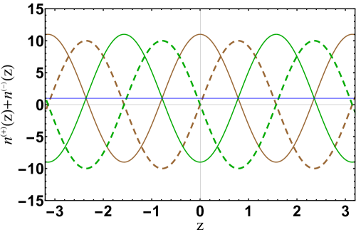
Figure 1: $n^{(+)}(z)+n^{(-)}(z)$ vs $z$ has been plotted. The brown lines show $n^{(+)}(z)$ and the green lines show $n^{(-)}(z)$. The solid lines represent the real part, and the dashed line represents the imaginary part. The blue line is the superposed profile of the two superpartner refractive indices. Here $v_{0}=10$ and $\beta=2$

Using (4.1) and (4.9), we thus arrive at the form

$$V^{(-)}=\gamma\Big{(}1-(cos{2\beta z}-\frac{2}{v_{0}}\cos{\beta z})\\ -i(\sin{2\beta z}-\frac{2}{v_{0}}\sin{\beta z})\Big{)}+\Lambda$$ (4.10)

where $\gamma=\frac{\beta^{2}v_{0}^{2}}{4}$, as a supersymmetric partner to $V^{(+)}$. The corresponding partner distribution of the refractive index reads $n^{(-)}(z)=n_{0}(1-v_{0}e^{i\beta z})$ in contrast to (27). An interesting off-shoot is that the supersymmetric partner indices add up to constant

$$n^{(+)}+n^{(-)}=2n_{0}$$ (4.11)

In [44], the relative permittivity distribution of the superpartner waveguide for a few profiles was identified. However, the basic analytical forms obtained in the present work for the partner potentials in the light of the complex splitting of the superpotential, along with the observation that the sum of the refractive indices corresponding to the supersymmetrically related distributions turning out to be a constant, are new. In the Figure 1 the individual variation of each refractive index is separately shown.

In Figure 2 we display a simple computation of the supersymmetric partner potentials. Specifically, we observe in Figure 2(a) that, while the real part of the original structure of $V^{(+)}$ depicts a repeated character of the multiple-well potential with narrow symmetrical drops, the shape of the imaginary part is also symmetrical in nature but passes through the origin. On the other hand, in Figure 2(b), for the plot of the partner $V^{(-)}$, the symmetrical nature of the multiple-well persists but, because of its mixed structure, there is a pronounced shift towards the positive $z$-axis in both the real part and the imaginary part.

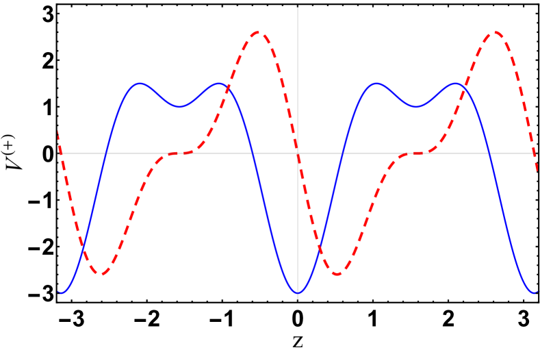
(a) $V^{(+)}$ vs $z$

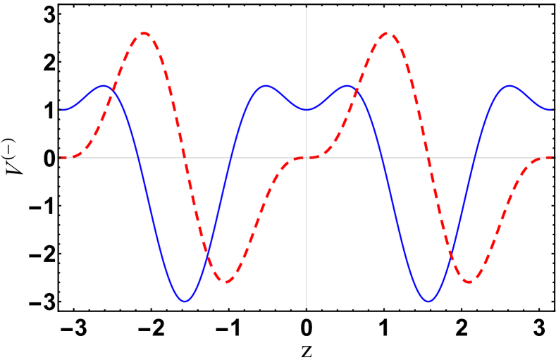
(b) $V^{(-)}$ vs $z$

Figure 2: Plots of $V^{\pm}$ vs $z$ where the solid blue line represents the real part of the potential and the dashed red line represents the respective imaginary part. Here $k=1$, $\Lambda=0$, and $v_{0}=1$.

4.2 The distribution $v(z)=\nu_{1}\cos 2\beta z+i\nu_{2}\sin 2\beta z$

This type of $v(z)$ follows from the $\mathcal{PT}$-symmetric periodic structure of the refractive index, $n^{(+)}(z)=\eta_{0}+\eta_{1}\cos{2\beta z}+i\eta_{2}\sin{2\beta z}$, where $\eta_{1}$ corresponds to the peak real index contrast and $\eta_{2}$ represents the gain and loss of the distribution. This form was recently advanced by Lin et al [36] to analyse the amplitudes of the forward and backward propagating waves outside of the grating domain and subsequently to acquire knowledge of the transmission and reflection coefficients. The purpose was to establish that $\mathcal{PT}$-symmetric periodic structures can act as unidirectional invisible media. Further, as a $\mathcal{PT}$-symmetric sinusoidal potential a similar form was studied in [58] as an acting potential to deal with the beam propagation in $\mathcal{PT}$-symmetric optical lattices while the phase transitions of the eigenvalues were earlier investigated in [59].

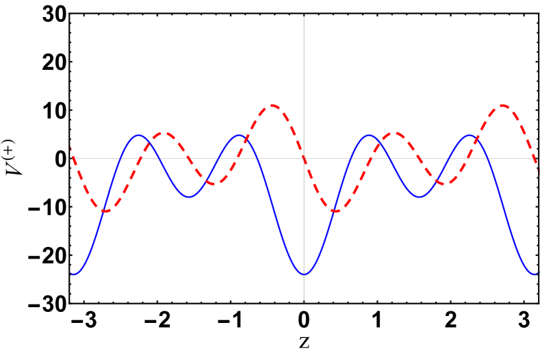
(a) $V^{(+)}$ vs $z$

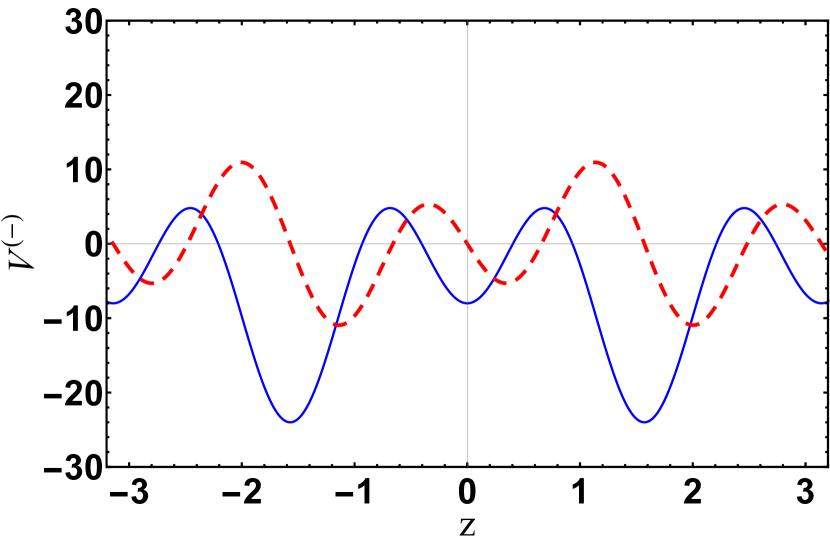
(b) $V^{(-)}$ vs $z$

Figure 3: Plots of $V^{\pm}$ vs $z$ where the solid blue line represents the real part of the potential and the dashed red line represents the respective imaginary part. Here $k=1$, $\Lambda=0$, $\nu_{1}=4$, and $\nu_{2}=2$.

Given the above distribution of the refractive index, we can utilize (4.2) to obtain

$$k^{2}\Big{(}1+\nu_{1}\cos{2\beta z}+i\nu_{2}\sin{2\beta z}\Big{)}^{2}=\varepsilon-\Lambda-(\mathcal{W}^{2}-\mathcal{W}^{\prime})$$ (4.12)

where $\nu_{1}=\frac{\eta_{1}}{\eta_{0}}$ and $\nu_{2}=\frac{\eta_{2}}{\eta_{0}}$. Then from (4.12) and (4.3), the corresponding real and imaginary part leads respectively to

$$k^{2}\Big{(}1+\nu_{1}^{2}\cos^{2}{2\beta z}-\nu_{2}^{2}\sin^{2}{2\beta z}\\ +2\nu_{1}\cos{2\beta z}\Big{)}=\varepsilon-f^{2}+g^{2}-f^{\prime}-\Lambda$$ (4.13a)

$$k^{2}\Big{(}2\nu_{1}\nu_{2}\cos{2\beta z}\sin{2\beta z}+2\nu_{2}\sin{2\beta z}\Big{)}=-2fg-g^{\prime}$$ (4.13b)

On inspection, the following set of solutions emerges

$$\beta=\pm k,\quad g=\nu_{2}\beta\cos{2\beta z},\quad f=-\nu_{1}\beta\sin{2\beta z}$$ (4.14)

along with

$$\varepsilon-\Lambda=k^{2}(1+\nu_{1}^{2}-\nu_{2}^{2})$$ (4.15)

and the superpartner wave-guide index acquires the form

$$n^{(-)}(z)=\eta_{0}\Big{(}1-\nu_{1}\cos{2\beta z}-i\nu_{2}\sin{2\beta z}\Big{)}$$ (4.16)

Here too the two index profiles satisfy the same constraint as in 4.11. The profiles of the corresponding $V^{(\pm)}$ are sketched in Figure 3. In contrast to the real part the imaginary part distinctly reveals a sinusoidal character with varying amplitudes.

5 Summary

In summary, we demonstrated that a modified uncertainty principle containing the Planck length $l_{P}$ and a dimensionless constant $\alpha$, when matched with the SHE, provides a lower bound for $\alpha$. We then subjected the SHE to a supersymmetric treatment within a $\mathcal{PT}$ optical structure in which the underlying refractive index distribution has a longitudinal variation. The superpartner of the index profile was analytically evaluated and closed form solutions of some typical distributions were obtained by solving a pair of coupled equation involving the real and imaginary components of the superpotential. The features of the index distribution corresponding to the supersymmetric partners were graphically illustrated.

6 Acknowledgements

Two of us (RG and SS) thank the Shiv Nadar IoE (deemed University) for financial assistance in the form of senior research fellowships.

References

- [1] A N Tawfik and A M Diab, Rep. Prog. Phys. 78, 126001 (2015)
- [2] D Gross and P Mende, Nucl.Phys. B303, 407 (1988)
- [3] D Amati, M Ciafaloni and G Veneziano, Phys. Lett. B216, 41 (1989)
- [4] L. Buoninfante, G. Gaetano Luciano and L. Petruzziello, Eur. Phys. J. C79, 663 (2019)
- [5] J.-L. Li and C.-F. Qiao, Ann. Phys. (Berlin) 533, 2000335 (2021)
- [6] P. Girdhar and A. C. Doherty, New J. Phys. 22, 093073 (2020)
- [7] B Bagchi and A Fring, Phys.Lett. A373, 4307 (2009)
- [8] M. Faizal and B. P. Mandal, Grav. and Cosm. 270 (2015)
- [9] S Hossenfelder, Living Rev.Rel. 16, 2 (2013)
- [10] M J Lake et al, Class. Quant. Grav. 36, 155012 (2019)
- [11] S. Das and E. C. Vagenas, Phys. Rev. Lett. 101, 221301 (2008)
- [12] P Bosso, S Das and R B. Mann, Phys. Lett. B 785, 498 (2018)
- [13] S Dey, Solvable Models on Noncommutative Spaces with Minimal Length Uncertainty Relations, PhD thesis, arXiv: 1410.3193 (hep-th)
- [14] L. M. Lawson, Sci Rep 12, 20650 (2022).
- [15] C Rovelli, Living Rev.Rel. 11, 5 (2008)
- [16] E. Witten, Phys. today 49, 24 (1996)
- [17] A. Kempf, Phys. Rev. Lett. 103, 231301 (2009)
- [18] M. Bojowald and A. Kempf, Phys. Rev. D86, 085017 (2012)
- [19] W. Heisenberg, Z. Phys. 43, 172 (1927)
- [20] E. H. Kennard, Z. Phys. 44, 326-52 (1927)
- [21] H. P. Robertson, Phys. Rev. 34, 163 (1929)
- [22] S. Kechrimparis and S. Weigert, Phys. Rev. A 90, 062118 (2014)
- [23] A Kempf, G Mangano and R B Mann, Phys.Rev. D52, 1108 (1995)
- [24] C Conti, Phys.Rev. A89, 061801 (2014)(R)
- [25] M. Maggiore, Phys. Rev. D 49, 5182 (1994)
- [26] R. J. Adler and D. I. Santiago, Mod. Phys. Lett. A 14, 1371 (1999)
- [27] R. J. Adler, P. Chen and D. I. Santiago, Gen. Rel. Grav. 33, 2101 (2001)
- [28] P. Chen and R. J. Adler, Nucl. Phys. Proc. Suppl. 124, 103 (2003)
- [29] R. J. Adler, Am. J. Phys. 78, 925 (2010)
- [30] F. Scardigli, Phys.Lett. B452, 39 (1999)
- [31] C. Bambi and F. R. Urban, Class. Quantum Gravity 25, 095006 (2008)
- [32] B. Carr, J. Mureika and P. Nicolini, JHEP 07, 052 (2015)
- [33] A A Zyablovsky, A P Vinogradov, A A Pukhov, A V Dorofeenko, A A Lisyansky, Physics - Uspekhi 57, 1063 (2014)
- [34] M C Braidotti, Z H Musslimani and C Conti, Physica D: Nonlinear Phenomena, 338, 34 (2017)
- [35] O. Steuernagel, Am. J. Phys. 73, 625 (2005)
- [36] Z. Lin, H. Ramezani, T. Eichelkraut, T. Kottos, H. Cao and D. N. Christodoulides, Phys. Rev. Let.. 106, 213901 (2011)
- [37] H. F. Jones, J. Phys. A: Math. Theor. 45, 135306 (2012)
- [38] H. F. Jones and M. Kulishov, J. Opt. 18, 055101 (2016)
- [39] Complex, transversely distributed refractive index which is inherently -symmetric and playing the role of an optical potential has been widely studied [40]. The corresponding electric-field envelope then obeys the paraxial equation of diffraction. For a study of the general class of index profiles see [41].
- [40] K. G. Makris, R. El-Ganainy and D. N. Christodoulides, Phys. Rev. Lett. 100, 103904 (2008).
- [41] A. Mostafazadeh, Phys. Rev. A92, 023831 (2015)
- [42] S. Longhi, J. Phys. (Math. Theor.), A44, 485302 (2011)
- [43] M.-A. Miri, M. Heinrich, R. El-Ganainy and D. N. Chritodoulides, Phys. Rev. Let. 110, 233902 (2013)
- [44] M.-A. Miri, Parity-time and supersymmetry in optics, PhD thesis (2014)
- [45] B. Mielnik and O. Rosas-Ortiz, J. Phys. (Math. Gen.) A37, 10007 (2004)
- [46] S.-H. Dong, Factorization method in quantum mechanics, Springer (Berlin), (2007)
- [47] A. A. Andrianov and M. V. Ioffe, J. Phys. (Math. Theor.), A45 503001 (2012)
- [48] D. Bermudez and D. J. Fernandez C., AIP Conf. Proc. 1575, 50 (2014)
- [49] G. Junker, Supersymmetric methods in quantum and statistical physics Springer, (Berlin) (1996)
- [50] B. Bagchi, Supersymmetry in quantum and classical mechanics (Chapman and Hall/CRC, Boca Raton) (2000)
- [51] F. Cooper, A. Khare and U. Sukhatme, Supersymmetry in quantum mechanics (World Scientific, Singapore) (2001)
- [52] A. Gangopadhyaya, J. Mallow and C. Rasinariu, Supersymmetric Quantum Mechanics: An Introduction (World Scientific, Singapore) (2017)
- [53] M.-L. Cai, Y.-K. Wu, Q.-X. Mei1, W.-D. Zhao, Y. Jiang, L. Yao1, L. He, Z.-C. Zhou and L.-M. Duan, Nature Comm. 13, 3412 (2022)
- [54] S M Chumakov, K B Wolf, Phys. Let. A193, 51 (1994)
- [55] A. A. Andrianov, M. V. Ioffe, F. Cannata and J.-P. Dedonder, Int. J. Mod. Phys. A14, 2675 (1999)
- [56] B Bagchi, S. Mallik and C. Quesne, Int. J. Mod. Phys. A 16, 2859 (2001)
- [57] M. Znojil, F. Cannata, B. Bagchi and R. Roychoudhury, Phys. Lett. B483, 284 (2000)
- [58] E.-M. Graefe and H. F. Jones, Phys. Rev. A 84, 013818 (2011)
- [59] B. Midya, B. Roy, and R. Roychoudhury, Phys. Lett. A 374, 2605 (2010)