Orthogonal separation of variables for spaces of constant curvature

Abstract

We construct all orthogonal separating coordinates in constant curvature spaces of arbitrary signature. Further, we construct explicit transformation between orthogonal separating and flat or generalised flat coordinates, as well as explicit formulas for the corresponding Killing tensors and Stäckel matrices.

MSC classes: 37J35, 70H20, 37J11, 37J06, 37J38, 70H15, 70S10, 37K06, 37K10, 37K25, 53B50, 53A20, 53B20, 53B30, 53B99

Key words: Separation of variables, finite-dimensional integrable systems, Hamilton-Jacobi equation, constant curvature spaces, Killing tensors, Stäckel matrix

1 Introduction

Physicists encounter separating variables at least in their first year at university. Indeed, a standard way of teaching physics is to suggest a mathematical model that may describe a physical phenomenon, find (partial, approximative) solutions to the model and compare them with known observations or experiments. The second step of this three-step procedure, finding and analysing mathematical solutions, often uses the separation of variables techniques, which in many cases allows one to reduce a multidimensional system of ODEs or PDEs describing the model to a system of uncoupled one-dimensional ODEs or even to algebraic or integro-algebraic equations and solve or analyse them effectively.

By (orthogonal) separation of variables on an $n$-dimensional pseudo-Riemannian manifold $(M,g)$ we understand the existence of a Killing tensor $K_{ij}$ such that the operator field $K^{i}_{j}$ has $n$ distinct eigenvalues and the Haantjes torsion of $K^{i}_{j}$ vanishes. These conditions imply the existence of local coordinates in which $K^{i}_{j}$, and hence $K_{ij}$ and $g_{ij}$, are all diagonal. These coordinates are called separating coordinates corresponding to $K$.

Recall that a symmetric $(0,2)$-tensor $K$ is a Killing tensor for $g$, if $\nabla_{(k}K_{ij)}=0$, where $\nabla$ is the Levi-Civita connection of $g$. Geometrically, this condition means that the function

$$I:TM\to\mathbb{R}\,,\ \ I(\xi)=K(\xi,\xi)$$

is constant along the orbits of the geodesic flow of $g$ (we refer to $I$ as the integral corresponding to $K$).

Our definition is equivalent to other definitions of orthogonal separation of variables used in the literature. Indeed, the existence of such a tensor $K_{ij}$ is equivalent to the (local) existence of $n$ Killing tensors $\overset{1}{K}_{ij}=g_{ij},\overset{2}{K}_{ij}=K_{ij},\overset{3}{K}_{ij},...,\overset{n}{K}_{ij}$ such that they are linearly independent and such that in the tangent space at almost every point there exists a basis in which all tensors $\overset{1}{K}_{ij},...,\overset{n}{K}_{ij}$ are diagonal, see e.g. [6, Proposition 2.2]. The integrals corresponding to these tensors Poisson commute. Moreover, in the separating coordinate system $(x^{1},...,x^{n})$, the tensors $\overset{1}{K}_{ij},...,\overset{n}{K}_{ij}$ have the so-called Stäckel form by [24]. In other words, there exists a nondegenerate $n\times n$ matrix $S=(S_{ij})$ with $S_{ij}$ being a function of the $i$-th variable $x^{i}$ only and such that the following condition holds:

$$SI=P,$$ (1)

where $I$ is an $n$-vector whose components are the integrals corresponding to $\overset{1}{K},...,\overset{n}{K}$, and $P=(p_{1}^{2},p_{2}^{2},...,p_{n}^{2})^{\top}$ is the $n$-vector of the squares of momenta. In this case, the Hamilton-Jacobi equation

$$\tfrac{1}{2}g^{ij}p_{i}p_{j}=c_{1}\,,\ p_{i}=\tfrac{\partial W}{\partial x^{i}}$$ (2)

admits (at a generic point) a general solution of the form

$$W(x,c)=\sum_{i=1}^{n}W_{i}(x^{i},c)\,,\ c=(c_{1},...,c_{n})\,,\ \det\left[\tfrac{\partial^{2}W}{\partial x^{i}\partial c_{j}}\right]\neq 0,$$

with $W_{i}(x^{i},c)=\pm\int^{x^{i}}\sqrt{\sum_{s}S_{is}(\xi)c_{s}}\operatorname{d}\xi$.

Having such a solution $W$, one can reduce integration of the geodesic flow to an algebraic problem: namely, in addition to the integrals $I_{1},...,I_{n}$, the functions $\tfrac{\partial W}{\partial c_{i}}$ with $i\neq 1$ are constant along any solution and, moreover, we have $t+\mathrm{const}=\tfrac{\partial W}{\partial c_{1}}$. Solving this system with respect to $x$ gives the general solution $x(t)$.

Note, however, that in many problems the primitives of $\pm\sqrt{\sum_{s}S_{is}c_{s}}$ cannot be obtained explicitly so that the relations $\tfrac{\partial W}{\partial c_{i}}=\mathrm{const}_{i},$ $t+\mathrm{const}=\tfrac{\partial W}{\partial c_{1}}$ form a system of integral-algebraic equations. In many cases one can still find exact solutions using special functions.

It is known that introducing potential energy does not pose essential difficulties: one simply replaces the vector $P=(p_{1}^{2},...,p_{n}^{2})^{\top}$ in (1) by $P+F=(p_{1}^{2}+f_{1}(x_{1}),...,p_{n}^{2}+f_{n}(x^{n}))^{\top}$ with arbitrary functions $f_{i}$. This gives an explicit formula $I=S^{-1}(P+F)=S^{-1}P+S^{-1}F$ for the commuting Hamiltonians. In particular, $H=I_{1}=\sum_{j}(S^{-1})_{1j}(p_{j}^{2})+\sum_{j}(S^{-1})_{1j}f_{j}$, where the latter term is a function on $M$ understood as a potential energy (such functions $U(x)=\sum_{j}(S^{-1})_{1j}f_{j}(x^{j})$ are called separable potentials).

In our paper, we will assume that $g$ has constant sectional curvature (and $M$ is connected). In this set-up, the above definition is equivalent to what is called multiplicative separation of variables in literature. Namely, by [18, 9], the second order differential operators

$$\overset{\alpha}{\mathcal{K}}:=\sum_{i,j}\nabla_{i}\overset{\alpha}{K}^{ij}\nabla_{j}$$

mutually commute and also commute with $\Delta_{g}=\overset{1}{\mathcal{K}}$. In the positive definite case and on compact manifolds (or under appropriate boundary assumptions), this implies that the Helmholtz partial differential equation $\Delta_{g}\phi=\lambda\phi$ and time independent Schrödinger equation $(\Delta_{g}+U(x))\phi=\lambda\phi$, where $U$ is a separable potential, can be reduced to a system of $n$ uncoupled ordinary differential equation by a multiplicative ansatz $\phi=\phi_{1}(x^{1})\phi_{2}(x^{2})\cdots\phi_{n}(x^{n})$.

Note that the condition that the sectional curvature of $g$ is constant appears naturally in physics, see e.g. [47]. Clearly, the flat metric is possibly the most important one for physical applications, and indeed, separation of variables for the flat metric was used in many physical problems, see e.g. [65, 66]. Metrics of nonzero sectional curvature are often used to describe phenomena near a point source (e.g., near an atomic nucleus or a star in the Universe, see e.g. [19, 23]).

An additional motivation comes from infinite dimensional integrable systems. It was observed [1, 10, 25, 64] that certain finite dimensional reductions of famous integrable PDE systems are equivalent (in the sense explained e.g. in [10]) to finite dimensional integrable systems coming from separation of variables for constant curvature metrics (of possibly indefinite signature). The relation to infinite dimensional integrable systems seems to be very deep and is far from being understood. As it will be clear from the discussion below, we came to this problem studying infinite dimensional compatible Poisson brackets [13, 15, 16]. Note also that separating coordinates are orthogonal and it is known, see e.g. [67], that orthogonal coordinates in flat spaces are closely related to infinite dimensional integrable systems. There also exists a clear relation between weakly nonlinear (=linearly degenerate) infinite dimensional integrable systems of hydrodinamic type and orthogonal separation of variables, see e.g. [17, 27, 35].

Because of their importance, (orthogonal) separating coordinates for metrics of constant curvature have been studied since at least the 19th century. In particular, it was known that in all dimensions and in all signatures, the ellipsoidal coordinates are separating for the pseudo-Riemannian spaces of constant curvature. It was also known that in low dimensions $n=2,3$ all separating coordinates can be constructed from ellipsoidal coordinates by passing to the limit, see [49, 50] and discussion in [34]. Note also that the orthogonality condition for separating coordinates can be weakened. However, as shown in [4] and [34], at least in the Riemannian signature, this more general case reduces naturally to a description of orthogonal separating coordinates.

In the series of fundamental works [31, 32, 33] E. Kalnins et al. suggested, in all dimensions and all signatures, a list of separating coordinates for metrics of constant sectional curvature. The list is parametrized by a combinatorial object which is a graph with some numerical labels. Moreover, in [31] it was claimed that this list contains all separating coordinates. The claim was not proved in [31], it was merely said that the proof is similar to that in the Riemannian case. The special case when the metric is Riemannian was indeed proved in [32, 33], see also [34]. To the best of our knowledge, a proof in the general case, when the metric has indefinite signature, did not appear in the literature. Although it was generally believed that the description in [31] is correct and complete. In particular, this is stated in [54, Theorem 1.3] but without proof. More precisely, [54, Theorem 1.3] consists of two statements. The first statement claims that for every separating coordinate system on a manifold of constant curvature, there exists a $(1,1)$-tensor $L$ which is diagonal in this coordinate system and which is geodesically compatible to the metric (see §3.1 for necessary definitions). This statement is proved. The existence of such a tensor allows one, in principle, to reduce the study of separating coordinate systems on $n$-dimensional manifold of constant curvature to low dimensional cases; applying this reduction recursively (see e.g. [55, 62, 63] for examples), one can construct all separating coordinate systems for spaces of constant curvature. However, neither comparison with the description of [31], nor explicit formulas for the metrics of constant curvature in separating coordinates are given in [53, 54, 55]. Note that the papers [62, 63] containing an explicit description assume $n=3$.

Our paper fills this gap and proves that the list from [31] is complete (see Theorem 1.1). Our description is visually different, but equivalent to the description in [31] and, we believe, has some advantages as compared to that used in [31] and further publications, e.g. [34, 53, 54, 55]; in particular, because it is given by explicit formulas rather than by a recursive algorithm.

We demonstrate the advantages of our approach with the following additional new results:

• We construct explicit formulas for flat and generalised flat coordinates as functions of separating coordinates, see Theorems 1.5, 1.6 and 1.7. Previously, only special cases were known, see e.g. [8, 31, 45].

• We prove the essential uniqueness of a $(1,1)$-tensor $L$ which is diagonal in the separating coordinate system and is geodesically compatible with the metric (see Theorem 3.1 and necessary definitions in §3.1). Such $(1,1)$-tensors play a key role in the algebraic approach to classification of separating coordinates for constant curvature spaces, see e.g. [56, 57, 58, 59], and also in the approach of [53, 54, 55, 62, 63]. We use the essential uniqueness of $L$ when discussing those cases where two sets of parameters describe equivalent separating coordinates, see Theorem 1.2.

• We construct Killing tensors and the corresponding Stäckel matrix (Theorems 1.3 and 1.4). These tasks were initiated in [31, p. 203] (but postponed for publication elsewhere).

In our proof, we show that the existence of separating coordinates can be reduced to a system of PDEs which was studied in our recent paper [15]. The motivation of [15] is very different from that of [31, 33]. The goal of [15] was to describe all compatible pencils of $\infty$-dimensional geometric Poisson structures of the form $\mathcal{P}_{3}+\mathcal{P}_{1}$ on the loop space, where $\mathcal{P}_{i}$ has order $i$ and $\mathcal{P}_{3}$ is Darboux-Poisson. We achieved this goal under natural nondegeneracy assumptions and obtained a full list of such structures; this list is also parametrized by a graph with labels. Then, we observed that our graph with labels and the description obtained in [31], although visually different, are actually combinatorially equivalent. This suggested that one could use the calculation and arguments of [15] to prove the claim of [31], and this is how we proceed in the current paper. First we explain how to reduce the system of PDEs describing the existence of separating coordinates to those equations which were studied and completely solved in [15]. Then we use this solution to prove the claim of [31]. Of course, a direct proof, without using [15] but repeating all the steps from [15], is also possible and we explain how it goes.

Let us emphasize that certain steps of the proof in the Riemannian case from [32, 33], in combination with [24] (or Appendix of [32]), resemble those from [15]. This makes us believe that E. Kalnins, W. Miller and G. Reid, the authors of [31], had the proof of their claim, but did not publish it due to its length and complexity. In fact, in the case of indefinite signature new phenomena appear and the proof becomes more complicated compared to the Riemannian case. Also note that the proof from [15] is quite long and complex.

Recall that by [28, 36], for a real-analytic metric and therefore for the metrics of constant curvature, any Killing tensor is also real-analytic. Therefore, a local existence of separating coordinates implies their existence near almost every point; moreover, separating coordinates can be chosen to be real-analytic.

Let us also note that we allow some coordinates to be complex-valued; the corresponding momenta are also complex-valued. We assume, of course, that along with a complex coordinate $z^{j}=x^{j}+ix^{j+1}$, its complex-conjugate $\bar{z}^{j}=x^{j}-ix^{j+1}$ is also a coordinate. Having formulas for the metric, Killing tensor, or separating ansatz in coordinates involving complex conjugate pairs $z^{j},\bar{z}^{j}$, it is straightforward to rewrite them in real-valued coordinates (see e.g. [21]).

1.1 Description of separating coordinates for metrics of constant curvature

We start with an explicit construction of a family of diagonal metrics in some coordinates. Our main result, Theorem 1.1, states that these coordinates are separating, the metrics have constant curvature, and any pair (metric of constant curvature, separating coordinate system) is contained in the family, modulo renumeration of coordinates and coordinate changes of the form $x_{\mathrm{\mathrm{new}}}^{i}=x_{\mathrm{\mathrm{new}}}^{i}(x_{\mathrm{\mathrm{old}}}^{i})$.

Each metric from the family is built based on the following data:

1. Natural number $B\leq n:=\dim M$  (=“number of blocks”).

2. Natural numbers $n_{1},...,n_{B}$ (=“dimensions of blocks”) with $\sum_{\alpha=1}^{B}n_{\alpha}=n$.

3. In-directed rooted forest $\mathsf{F}$ (with $B$ vertices which we denote by numbers $1,...,B$), that is, an oriented graph such that each of its connected component is a rooted tree and for any vertex there exists a necessarily unique oriented path towards a root. The edge of the graph connecting vertices $\beta$ and $\alpha$ and oriented towards $\alpha$ will be denoted by $\vec{\beta\alpha}$. An example of a rooted tree with $B=4$ vertices is on Figure 1.

   

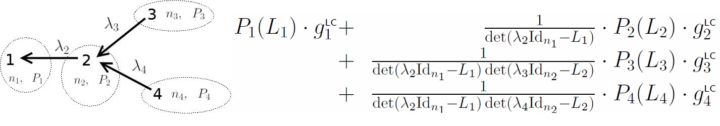
   Figure 1: An example of an in-tree, structure of its labels and the form of the corresponding metric (5).

4. Each edge $\vec{\beta\alpha}$ of $\mathsf{F}$ is labelled by a number $\lambda_{\beta}$.

5. Polynomials $P_{\alpha},$ $\alpha=1,...,B$ of degree at most $n_{\alpha}+1$, whose coefficients are denoted as follows:

   $$P_{\alpha}(t)=\overset{\alpha}{a}_{0}+\overset{\alpha}{a}_{1}t+...+\overset{\alpha}{a}_{n_{\alpha}+1}t^{n_{\alpha}+1}.$$

The structure of an in-directed forest defines a natural strict partial order (denoted by $\prec$) on the set $\{1,...,B\}$: for two numbers $\alpha\neq\beta\in\{1,...,B\}$ we set $\alpha\prec\beta$, if there exists an oriented path from $\beta$ to $\alpha$. For instance, for the graph shown on Figure 1, we have $1\prec 2\prec 3$, $1\prec 2\prec 4$. We say $\alpha=\operatorname{next}(\beta)$, if the graph contains the edge $\vec{\beta\alpha}$. In Figure 1, the root is $1$, the leaves are $3$ and $4$ and we have: $1=\textrm{next}(2)$, $2=\textrm{next}(3)$, $2=\textrm{next}(4)$.

Further, we assume that the polynomials $P_{\alpha}$ and numbers $\lambda_{\beta}$ satisfy the following restrictions:

• If $\mathsf{F}$ has more than one connected component and therefore more that one root, then for any root $\alpha$ we have $\overset{\alpha}{a}_{n_{\alpha}+1}=0$, i.e., $\deg P_{\alpha}\leq n_{\alpha}$.

• If $\alpha=\operatorname{next}(\beta)$, then $\lambda_{\beta}$ is a root of $P_{\alpha}$ and $\overset{\beta}{a}_{n_{\beta}+1}=P_{\alpha}^{\prime}(\lambda_{\beta})$, where $P^{\prime}(t)$ denotes the derivative of $P(t)$.

• If for at least two vertices $\beta\neq\gamma$ we have $\operatorname{next}(\beta)=\operatorname{next}(\gamma)=:\alpha$ with $\lambda_{\beta}=\lambda_{\gamma}=:\lambda$, then $\lambda$ is a double root of $P_{\alpha}$. Note that in view of (ii) this automatically implies $\overset{\beta}{a}_{n_{\alpha}+1}=\overset{\gamma}{a}_{n_{\gamma}+1}=0$.

Based on these data, we construct the following diagonal metric $g$. We first divide our diagonal coordinates into $B$ blocks of dimensions $n_{1},...,n_{B}$ with $n_{1}+...+n_{B}=n$:

$$(\underbrace{x_{1}^{1},...,x_{1}^{n_{1}}}_{X_{1}},...,\underbrace{x_{B}^{1},...,x_{B}^{n_{B}}}_{X_{B}}).$$ (3)

Next, for every $\alpha=1,...,B$ we consider the $n_{\alpha}$-dimensional contravariant metric $g^{\mbox{\tiny{\sf LC}}}_{\alpha}$ and $n_{\alpha}$-dimensional operator (= $(1,1)$-tensor) $L_{\alpha}$ given by:

$$g^{\mbox{\tiny{\sf LC}}}_{\alpha}=\sum_{s=1}^{n_{\alpha}}\left(\prod_{j\neq s}(x_{\alpha}^{s}-x_{\alpha}^{j})\right)^{-1}\left(\tfrac{\partial}{\partial x_{\alpha}^{s}}\right)^{2}\ \ ,\ \ L_{\alpha}=\textrm{diag}(x_{\alpha}^{1},...,x_{\alpha}^{n_{\alpha}}).$$ (4)

Finally, we introduce a diagonal metric

$$g=\operatorname{diag}(g_{1},\dots,g_{B})\quad\mbox{with }g_{\alpha}=f_{\alpha}\cdot P_{\alpha}(L_{\alpha})\cdot g^{\mbox{\tiny{\sf LC}}}_{\alpha},$$ (5)

and $f_{\alpha}$ given by

$$f_{\alpha}=\prod_{\begin{array}[]{c}s\stackrel{{\scriptstyle\prec}}{{=}}\alpha\\ \textrm{$s$ not a root}\end{array}}\frac{1}{\det(\lambda_{s}\cdot\operatorname{Id}_{n_{s}}-L_{\operatorname{next}(s)})},$$ (6)

where $s\stackrel{{\scriptstyle\prec}}{{=}}\alpha$ means that $s\prec\alpha$ or $s=\alpha$ and $\operatorname{Id}_{n_{s}}$ denotes the identity operator in dimension $n_{s}$. If $\alpha$ is a root, we set $f_{\alpha}=1$. We also use $P_{\alpha}(L_{\alpha})$ for the polynomial $P_{\alpha}$ applied to the operator $L_{\alpha}$. Since $L_{\alpha}=\operatorname{diag}(x_{\alpha}^{1},...,x_{\alpha}^{n_{\alpha}})$, we simply have $P_{\alpha}(L_{\alpha})=\operatorname{diag}\bigl{(}P_{\alpha}(x_{\alpha}^{1}),...,P_{\alpha}(x_{\alpha}^{n_{\alpha}})\bigr{)}$. Similarly, $P_{\alpha}(L_{\alpha})\cdot g^{\mbox{\tiny{\sf LC}}}_{\alpha}$ is the product of the diagonal matrices $P_{\alpha}(L_{\alpha})$ and $g^{\mbox{\tiny{\sf LC}}}_{\alpha}$. See Figure 1 for an example. See also [15, first formula for $g$ in Example 4.1] for an example with flat $g$ and $B=n_{1}=n_{2}=2$.

This completes the description of the family of (contravariant) metrics and we can state our main result.

Theorem 1.1.

The metrics (5) have constant sectional curvature and $x^{1},...,x^{n}$ are separating coordinates for them. Moreover, every pair (metric of constant curvature, separating coordinates for it) can be brought to this form by renumeration of coordinates and coordinate transformations of the form $x_{\mathrm{new}}^{i}=x_{\mathrm{new}}^{i}(x_{\mathrm{old}}^{i})$, $i=1,\dots,n$.

The curvature of the metric $g$ given by (5) is $-\tfrac{1}{4}\overset{\alpha}{a}_{n_{\alpha}+1}$, where $\alpha$ is a root of the forest $\mathsf{F}$. Note that if $\mathsf{F}$ has several connected components, then the curvature is zero by (i). In this case, $g$ is the direct product of the metrics corresponding to the connected components.

1.2 What parameters describe equivalent separating coordinates?

Let us now discuss when two different sets of parameters (in-directed rooted forest $\mathsf{F}$, numbers $B$, $n_{\alpha}$, $\lambda_{\beta}$, and polynomials $P_{\alpha}$ satisfying conditions (i)–(iii) from §1.1) describe the same separating coordinates (of a fixed metric of constant curvature) up to the following freedom: re-numeration of coordinates and coordinate changes of the form $x^{i}_{\mathrm{new}}=x^{i}_{\mathrm{new}}(x^{i}_{\mathrm{old}})$.

Clearly, if one set of data can be obtained from another by the operations described below, then the corresponding separating coordinates, in the above sense, coincide:

• For some $\alpha\in\{1,...,B\}$, we re-numerate (via a bijection from $\{1,...,n_{\alpha}\}$ to itself) the coordinates in the coordinate block $X_{\alpha}=(x_{\alpha}^{1},...,x_{\alpha}^{n_{\alpha}})$.

• For some $\alpha\in\{1,...,B\}$, in the coordinate block $X_{\alpha}=(x_{\alpha}^{1},...,x_{\alpha}^{n_{\alpha}})$, we change the variables by the formula ${\overset{\mathrm{new}}{x}}{}_{\alpha}^{i}=A{\overset{\mathrm{old}}{x}}{}_{\alpha}^{i}+C$ with constants $A\neq 0$ and $C$, and “compensate” this as follows:

  • Change the polynomial $P_{\alpha}(t)$ by the polynomial $A^{n_{\alpha}+1}P_{\alpha}\left(\tfrac{t-C}{A}\right)$.

  • For each $\beta$ such that $\operatorname{next}(\beta)=\alpha$, change the number $\lambda_{\beta}$ by $A\lambda_{\beta}+C$.

  • For each $\gamma$ such that the oriented path from $\gamma$ to the root passes through $\alpha$, multiply the polynomial $P_{\gamma}$ by $A^{n_{\alpha}}$.

• Rename the vertices in the in-directed forest (via a bijection from $\{1,...,B\}$ to itself).

• If $\alpha$ is a leaf (= no incoming edges) and $n_{\alpha}=1$, replace the polynomial $P_{\alpha}$ by any other polynomial $\tilde{P}_{\alpha}$ satisfying conditions (i)–(iii) such that the sign of $P_{\alpha}(x_{old})$ coincides with that of $\tilde{P}_{\alpha}(x_{new})$.

It is easy to check that the operations do not destroy conditions (i)–(iii) of §1.1. The next theorem says that these operations exhaust all possibilities.

Theorem 1.2.

Suppose two sets of admissible data $($in-directed rooted forest $\mathsf{F}$, numbers $B$, $n_{\alpha}$, $\lambda_{\beta}$, and polynomials $P_{\alpha}$ satisfying conditions (i)–(iii) from §1.1$)$ describe the same separating coordinates up to re-numeration of coordinates and transformations of the form $x^{i}_{\mathrm{new}}=x^{i}_{\mathrm{new}}(x^{i}_{\mathrm{old}})$. Then one of the sets of admissible data can be transformed into the other one using a finite number of operations (A), (B), (C), (D) described above.

Remark 1.1.

One can use operations (B) and (D) to reduce the number of parameters in the labelling of $\mathsf{F}$.

1.3 Killing tensors in separating coordinates and the corresponding Stäckel matrix

The existence of Killing tensors for metric (5) that are diagonal in the coordinates $(x^{1},...,x^{n})$ will be clear from the proof. The goal of this section is to give an explicit formula for these Killing tensors.

As a by-product (Theorem 1.4) we obtain an explicit formula for the Stäckel matrix. This result is important from the point of view of applications: indeed, as recalled in Introduction, the solution $W(x,c)$ of the Hamilton-Jacobi equation corresponding to separating coordinates involves the Stäckel matrix. Note also that in [31, p. 203] Kalnins et al. explicitly asked to construct the Stäckel matrices corresponding to separating variables on spaces of constant curvature.

Following [11, 40] (see also Facts 3.2, 3.3 from §3.1), we recall the construction of Killing tensors for the Levi-Civita metric (4). Consider the following family $\overset{\alpha}{S}_{\mbox{\tiny{\sf LC}}}(t_{\alpha})$ of $(1,1)$ tensors on the $\alpha$-block with coordinates $X_{\alpha}=(x_{\alpha}^{1},...,x_{\alpha}^{n_{\alpha}})$:

$$\overset{\alpha}{S}_{\mbox{\tiny{\sf LC}}}(t_{\alpha})=\left(t_{\alpha}\operatorname{Id}_{n_{\alpha}}-L_{\alpha}\right)^{-1}\det\left(t_{\alpha}\operatorname{Id}_{n_{\alpha}}-L_{\alpha}\right).$$ (7)

Note that $\overset{\alpha}{S}_{\mbox{\tiny{\sf LC}}}(t_{\alpha})$ is polynomial of degree $n_{\alpha}-1$ in $t_{\alpha}$. It is known, see e.g. [11], that for every $t_{\alpha}$ the $(0,2)$-tensor $\overset{\alpha}{K}{}^{\mbox{\tiny{\sf LC}}}_{ij}$ given, for any two tangent vectors $\xi,\eta$, by

$$\overset{\alpha}{K}{}^{\mbox{\tiny{\sf LC}}}(\xi,\eta)={g}^{\mbox{\tiny{\sf LC}}}_{\alpha}(\overset{\alpha}{S}_{\mbox{\tiny{\sf LC}}}(t_{\alpha})\xi,\eta)$$ (8)

is a Killing tensor for ${g}^{\mbox{\tiny{\sf LC}}}_{\alpha}$. Clearly, the number of linearly independent Killing tensors within the family (8) is $n_{\alpha}$ and generically they have $n_{\alpha}$ different eigenvalues.

Next, with the help of the family of Killing tensors $\overset{\alpha}{K}{}^{\mbox{\tiny{\sf LC}}}$ of the $n_{\alpha}$ dimensional metric $g_{\alpha}^{\mbox{\tiny{\sf LC}}}$, let us construct Killing tensors for the metric $g=\operatorname{diag}(g_{1},\dots,g_{B})$ given by (5). We first define the (1,1)-tensor $\overset{\alpha}{S}(t_{\alpha})$ to be block-diagonal in the coordinates $(x^{1},...,x^{n})=(X_{1},...,X_{B})$ with the following blocks:

• the $\alpha$-block ($\alpha\in\{1,\dots,B\}$) is $\overset{\alpha}{S}_{\mbox{\tiny{\sf LC}}}/f_{\alpha}$, where $\overset{\alpha}{S}_{\mbox{\tiny{\sf LC}}}$ is given by (7) and $f_{\alpha}$ by (6);

• every $\beta$-block with $\alpha\prec\beta$ is given by

  $$\overset{\alpha\beta}{\Phi}(t_{\alpha})\operatorname{Id}_{n_{\beta}},$$

  where $\overset{\alpha\beta}{\Phi}$ is the polynomial in $t_{\alpha}$ of degree $n_{\alpha}-1$ given by

  $$\overset{\alpha\beta}{\Phi}(t_{\alpha}):=\tfrac{1}{t_{\alpha}-\lambda_{\gamma}}\tfrac{1}{f_{\alpha}}\bigl{(}\det(t_{\alpha}\operatorname{Id}_{n_{\alpha}}-L_{\alpha})-\det(\lambda_{\gamma}\operatorname{Id}_{n_{\alpha}}-L_{\alpha})\bigr{)},$$ (9)

  where $\gamma$ is such that $\gamma\prec\beta$ or $\gamma=\beta$ and $\operatorname{next}(\gamma)=\alpha$ (these conditions determine $\gamma$ uniquely;

• for every other $\mu\in\{1,\dots,B\}$, the corresponding $\mu$-block is zero.

Theorem 1.3.

For every $\alpha$ and $t_{\alpha}$ the $(0,2)$-tensor $\overset{\alpha}{K}(t_{\alpha})$ given, for any two tangent vectors $\xi,\eta$, by

$$\overset{\alpha}{K}(t_{\alpha})(\xi,\eta)=g(\overset{\alpha}{S}(t_{\alpha})\xi,\eta)$$ (10)

is a Killing tensor for $g$. Moreover, for any $\alpha,\beta$ and any $t_{\alpha}$, $t_{\beta}$ the integrals corresponding to the Killing tensors $\overset{\alpha}{K}(t_{\alpha})$ and $\overset{\beta}{K}(t_{\beta})$ Poisson-commute.

Clearly, the space spanned by each individual family $\overset{\alpha}{K}(t_{\alpha})$ is $n_{\alpha}$-dimensional, and the spaces spanned by different families $\overset{\alpha_{i}}{K}(t_{\alpha_{i}})$ are mutually independent, so that they span a vector space of dimension $n_{1}+...+n_{B}=n$.

Let us now describe the integrals from Theorem 1.3 by a Stäckel matrix, that is, find an $n\times n$ matrix $S$ such that the integrals corresponding to the Killing tensors are given by the “Stäckel” formula

$$SI=P,$$ (11)

where $I=(I_{1},...,I_{n})^{\top}$ is the $n$-vector whose components are integrals corresponding to the Killing tensors and $P=(p_{1}^{2},...,p_{n}^{2})^{\top}$ is the vector of squares of momenta. Recall that the $(i,j)$-component $S_{ij}$ is a function of $x^{i}$ only and this property implies Poisson commutativity of the components of $I$.

As specific Killing tensors related to the integrals $I_{1},\dots,I_{n}$, we take the coefficients of the polynomials $\overset{\alpha}{K}(t_{\alpha})$. Namely, the first Killing tensor is the coefficient of $\overset{1}{K}(t_{1})$ at $t_{1}^{n_{1}-1}$, the second Killing tensor is the coefficient of $\overset{1}{K}(t_{1})$ at $t_{1}^{n_{1}-2}$, …, the $n_{1}$-th Killing tensor is the free term of $\overset{1}{K}(t_{1})$, the $(n_{1}+1)$-st Killing tensor is the coefficient of $\overset{2}{K}(t_{2})$ at $t_{2}^{n_{2}-2}$ and so on.

We will see that the part of the matrix $S$ which is relevant for the integrals coming from the family $\overset{\alpha}{K}(t_{\alpha})$ corresponds to the coordinate block $X_{\alpha}$, that is, contains the rows from $n_{1}+...+n_{\alpha-1}+1$ to $n_{1}+...+n_{\alpha}.$ This part of the matrix is naturally divided into $B$ blocks of dimensions $n_{1}\times n_{\alpha}$, $n_{2}\times n_{\alpha}$,…, $n_{B}\times n_{\alpha}$. The following theorem describes them.

Theorem 1.4.

The block number $\alpha$ is a square $n_{\alpha}\times n_{\alpha}$ matrix whose $(i,j)$ element is given by $\frac{1}{P_{\alpha}(x_{\alpha}^{i})}\left(x_{\alpha}^{i}\right)^{n_{\alpha}-j}$. The block number $\beta$ with $\beta\neq\alpha$ is given as follows:

• it is zero if $\beta\neq\operatorname{next}(\alpha)$;

• for $\beta=\operatorname{next}(\alpha)$ the $i$-th component of the first column of the block is $\frac{1}{P_{\beta}(x_{\beta}^{i})(x_{\beta}-\lambda_{\beta})}$ and all the other columns are zero.

For example, for ${\mathsf{F}}=\left(1\overset{\lambda_{2}}{\longleftarrow}2\right)$ with two blocks of dimensions $n_{1}=3$ and $n_{2}=2$, the matrix $S$ is the product of two matrices:

$$S=\left(\begin{array}[]{ccccc}P_{1}(x^{1})&0&0&0&0\\ 0&P_{1}(x^{2})&0&0&0\\ 0&0&P_{1}(x^{3})&0&0\\ 0&0&0&P_{2}(x^{4})&0\\ 0&0&0&0&P_{2}(x^{5})\end{array}\right)^{-1}\left(\begin{array}[]{ccccc}(x^{1})^{2}&x^{1}&1&\frac{1}{x^{1}-\lambda_{2}}&0\\ (x^{2})^{2}&x^{2}&1&\frac{1}{x^{2}-\lambda_{2}}&0\\ (x^{3})^{2}&x^{3}&1&\frac{1}{x^{3}-\lambda_{2}}&0\\ 0&0&0&x^{4}&1\\ 0&0&0&x^{5}&1\end{array}\right).$$

The proof of Theorem 1.4 is an exercise in linear algebra and is left to the reader: one needs to invert the matrix $S$ from Theorem 1.4 and check that the rows give coefficients of the Killing tensors from Theorem 1.3.

1.4 Transformation between separating and (generalised) flat coordinates

We consider a metric $g$ given by (5) in coordinates $x^{1},...,x^{n}$ and assume first that it is flat. Following terminology in [2], we say that local functions $Y^{1}(x^{1},...,x^{n}),...,Y^{n}(x^{1},...,x^{n})$ form a flat coordinate system for $g$, if they are linearly independent and for every $i$ we have $\nabla\nabla Y^{i}=0$, where $\nabla$ is the Levi-Civita connection of $g$.

In the case of a metric $g$ of constant nonzero curvature $K$, by generalised flat coordinates we understand $n+1$ linearly independent local functions $Y^{1},...,Y^{n+1}$ such that for every $i\in\{1,...,n+1\}$ we have

$$\nabla\nabla Y^{i}+KY^{i}g=0.$$ (12)

In order to explain this terminology, for a metric $g=g_{ij}$ on $M$ consider the cone $\widehat{M}:=\mathbb{R}_{>0}\times M$ with the (covariant) metric $\widehat{g}=\tfrac{1}{K}(\operatorname{d}r)^{2}+r^{2}\sum_{i,j=1}^{n}g_{ij}\operatorname{d}x^{i}\operatorname{d}x^{j}$, where $r$ is the coordinate on $\mathbb{R}_{>0}$. If $g$ has constant curvature $K$, then the metric $\widehat{g}$ is flat. It is known and easy to check that the function $Y$ on $M$ satisfies (12) if and only if the function $\widehat{Y}:=rY$ on $\widehat{M}$ satisfies $\widehat{\nabla}\widehat{\nabla}\widehat{Y}=0$. In other words, $n+1$ functions $Y^{1},...,Y^{n+1}$ on $(M,g)$ form generalised flat coordinates, if and only if the functions $\widehat{Y}^{1}:=rY^{1},...,\widehat{Y}^{n+1}:=rY^{n+1}$ form flat coordinates on $(\widehat{M},\widehat{g})$.

Remark 1.2.

Equivalently, (generalised) flat coordinates $Y^{1},Y^{2},...$ for a (contravariant) metric $g$ of curvature $K$ can be characterised by the condition

$$g^{*}(\operatorname{d}Y^{i},\operatorname{d}Y^{j})=G^{ij}-KY^{i}Y^{j},$$

where $G=\Bigl{(}G^{ij}\Bigr{)}$ is a constant non-degenerate matrix of size $n\times n$, if $g$ is flat, and $(n+1)\times(n+1)$, if $K\neq 0$. In the latter case, $G^{ij}=\widehat{g}^{ij}$, where $\widehat{g}$ is the cone metric in the coordinates $rY^{1},...,rY^{n+1}$.

The importance of flat and generalised flat coordinates is clear. In mathematical physics, most problem are initially given in a flat or generalised flat coordinate system. Separation of variables method is used to find solutions of the corresponding ODEs/PDEs which are naturally given in separating coordinates. In order to compare them with observations or an experiment, one typically should transform them to the initial (generalised) flat coordinate system.

Remark 1.3.

We will also use the existence of (generalised) flat coordinates in the proof of Theorem 1.1. Namely, the existence of flat or generalised flat coordinates implies that the metrics given by (5) have constant curvature which is the first statement of Theorem 1.1.

In this section we describe flat and generalised flat coordinate system for the metrics $g$ given by (5) together with the corresponding matrix $G^{ij}$ (see Remark 1.2). We start with the case when $\mathsf{F}$ contains only one vertex, so that the (contravariant) metric $g$ has the form $P(L)g_{\mathsf{\mathsf{LC}}}$ with a polynomial $P$ of degree at most $n+1$.

1.4.1 Flat and generalised flat coordinates for the metric $P(L)g_{\mathsf{LC}}$

We start with the flat case, when $P$ has degree at most $n$. In this case, $g=P(L)g_{\mathsf{LC}}$ is flat.

Theorem 1.5.

Assume $P(t)=-4\,c\,(t-\mu_{1})^{k_{1}}(t-\mu_{2})^{k_{2}}...(t-\mu_{m})^{k_{m}}$ with $d:=n-(k_{1}+...+k_{m})\geq 0$ and mutually different $\mu_{i}$. Then, for every $i\in\{1,...,m\}$ and $\alpha\in\{0,...,k_{i}-1\}$ the function

$$Y_{i}^{\alpha}:=\tfrac{1}{\alpha!}\tfrac{\operatorname{d}^{\alpha}}{\operatorname{d}t^{\alpha}}\sqrt{\det(t\cdot{\operatorname{Id}}-L)}_{|t=\mu_{i}}$$ (13)

has the property $\nabla\nabla X_{i}^{\alpha}=0$. Moreover, the functions

$$Y_{\infty}^{\alpha}:=\tfrac{1}{\alpha!}\tfrac{\operatorname{d}^{\alpha}}{\operatorname{d}t^{\alpha}}\sqrt{\det(\operatorname{Id}-t\cdot{L})}_{|t=0}-R^{(\alpha)}$$ (14)

with $\alpha=1,...,d$ also have the property $\nabla\nabla Y_{\infty}^{\alpha}=0$. The constants $R^{\alpha}$ are defined as follows

$$R^{(\alpha)}=\tfrac{1}{\alpha!}\tfrac{\operatorname{d}^{\alpha}}{\operatorname{d}t^{\alpha}}\prod_{i=1}^{m}(1-t\mu_{i})^{k_{i}}{}_{|t=0}.$$ (15)

These $n$ functions

$$Y^{1}:=Y_{1}^{0},...,Y^{k_{1}}:=Y_{1}^{k_{1}-1},Y^{k_{1}+1}:=Y_{2}^{0},...,Y^{k_{1}+k_{2}}:=Y_{2}^{k_{2}-1},...,Y^{n-d+1}:=Y_{\infty}^{1},...,Y^{n}:=Y_{\infty}^{d}$$

are linearly independent and form flat coordinates for the contravariant metric $g=P(L)g_{\mathsf{LC}}$.

According to our literature research, the following special cases of Theorem 1.5 were known. The classically known case is when the polynomial $P$ has only simple roots (see Example 1.1). The case $P(t)=t^{k}$, $k=0,...,n$ (see Example 1.2) is solved in [8]. A discussion of the general case from the viewpoint of the limit procedure can be found in [31] and in particular, the case when $P$ has one double root and other roots are simple is given there with explicit formulas.

Remark 1.4.

Calculations in the proof of Theorem 1.5 also give us the matrix of the contravariant metric $g=P(L)g_{\mathsf{LC}}$ in coordinates $Y^{1},...,Y^{n}$. It is blockdiagonal with $m+1$ blocks of dimensions $k_{1},...,k_{m},d$. The $i$-th block with $i=1,...,m$ is the product of $k_{i}\times k_{i}$ matrices $\widehat{P}_{i}(J+\mu_{i}\cdot\operatorname{Id})$ and $c\cdot A$, where $\widehat{P}_{i}(t)=\prod_{s\neq i}(t-\mu_{s})^{k_{s}}$, and the matrices $J$ (“Jordan block”) and $A$ (“antidiagonal matrix”) are given by

$$J=\begin{pmatrix}0&0&\cdots&\cdots&0\\ 1&0&0&\cdots&0\\ 0&1&\ddots&\ddots&\vdots\\ \vdots&\ddots&\ddots&\ddots&0\\ 0&0&\cdots&1&0\end{pmatrix}\ \ \textrm{and}\ \ A=\begin{pmatrix}0&\cdots&\cdots&0&1\\ 0&\cdots&0&1&0\\ \vdots&\mathinner{\mkern 1.0mu\raise 1.0pt\vbox{\kern 7.0pt\hbox{.}}\mkern 2.0mu\raise 4.0pt\hbox{.}\mkern 2.0mu\raise 7.0pt\hbox{.}\mkern 1.0mu}&\mathinner{\mkern 1.0mu\raise 1.0pt\vbox{\kern 7.0pt\hbox{.}}\mkern 2.0mu\raise 4.0pt\hbox{.}\mkern 2.0mu\raise 7.0pt\hbox{.}\mkern 1.0mu}&0&\vdots\\ 0&\mathinner{\mkern 1.0mu\raise 1.0pt\vbox{\kern 7.0pt\hbox{.}}\mkern 2.0mu\raise 4.0pt\hbox{.}\mkern 2.0mu\raise 7.0pt\hbox{.}\mkern 1.0mu}&\mathinner{\mkern 1.0mu\raise 1.0pt\vbox{\kern 7.0pt\hbox{.}}\mkern 2.0mu\raise 4.0pt\hbox{.}\mkern 2.0mu\raise 7.0pt\hbox{.}\mkern 1.0mu}&\vdots&0\\ 1&0&\cdots&0&0\end{pmatrix}.$$

The $(m+1)$-st block is the product of $d\times d$ matrices $-\widehat{P}_{\infty}(J)$ and $c\cdot A$, were $\widehat{P}_{\infty}(t)=\prod_{s}({1-t\mu_{s}})^{k_{s}}$.

Remark 1.5.

Some of the flat coordinates $Y^{k}$ can be complex-valued. This may be related to complex roots $\mu_{i}$, or can appear if $\mu_{i}$ is real but $\det(\mu_{i}\cdot\operatorname{Id}-L)<0$. In the first case, the real and the imaginary parts of the complex-valued coordinates contribute to real flat coordinates. In the second case, the square root and its derivatives are pure imaginary at the point $\mu_{i}$. The imaginary parts of them give real coordinates. Note that the matrix of $g^{ij}$ in the flat coordinates $Y^{k}$ from Remark 1.4 is calculated as the matrix of scalar products of the differentials $\operatorname{d}Y^{i}$ and $\operatorname{d}Y^{j}$, in particular if $Y^{i}$ and $Y^{j}$ are purely imaginary the $g$-scalar product of the corresponding differentials is minus the $g$-scalar product of the differentials of the corresponding imaginary parts. In other words, when we pass from the pure imaginary coordinates to their imaginary parts we should multiply the corresponding blocks of the matrix from Remark 1.4 by $-1$.

Let us recall two known examples: Example 1.1 is classical and Example 1.2 can be found in [8, 45].

Example 1.1.

Assume the polynomial $P=-4\prod_{i=1}^{n}(t-\mu_{i})$ has $n$ simple real roots $\mu_{1}<...<\mu_{n}$. Then,

$$Y^{i}=\sqrt{\det(\mu_{i}\operatorname{Id}-L)}=\sqrt{\prod_{s=1}^{n}(\mu_{i}-x^{s})}.$$

In these coordinates, the matrix of $g$ is diagonal: $g_{ij}=\operatorname{diag}\left(\prod_{s\neq 1}(\mu_{1}-\mu_{s}),\dots,\prod_{s\neq n}(\mu_{n}-\mu_{s})\right)$. After the cosmetic change of the form

$$Y_{\mathrm{new}}^{i}=\frac{Y_{\mathrm{old}}^{i}}{\sqrt{\prod_{s\neq i}(\mu_{i}-\mu_{s})}}\ \ \ \left(=\sqrt{\frac{\prod_{s=1}^{n}(\mu_{i}-x^{s})}{\prod_{s\neq i}(\mu_{i}-\mu_{s})}}\right)$$ (16)

the metric takes the form $g=\operatorname{diag}(\pm 1,\dots,\pm 1)$.

In particular, if the metric is Riemannian, the polynomial $P$ necessarily has $n$ or $n-1$ real simple root and the range of the coordinates is as follows: $\mu_{1}<x^{1}<\mu_{2}<\cdots<\mu_{n}<x^{n}$ (in the case of $n-1$ simple roots we think that $\mu_{1}=-\infty$). In this case, the coordinates $Y_{\mathrm{new}}^{i}$ are real-valued and the metric $g$ in these coordinates is the standard Euclidean metric. Formula (16), known since Jacobi [30] and Neumann [48], expresses Cartesian coordinates $Y^{i}$ in terms of ellipsoidal coordinates $x^{i}$ and is widely used in many physical applications.

Example 1.2.

If $P(t)=t^{n}$, the flat coordinates are coefficients of the characteristic polynomial of $L$:

$$\det(t\cdot\operatorname{Id}-L)=t^{n}+Y^{n}t^{n-1}+Y^{n-1}t^{n-2}+...+Y^{1}.$$ (17)

In the coordinates $Y^{i}$, the matrix of $g$ is the antidiagonal matrix $A$ from Remark 1.4.

Next, let us consider the case of metrics $P(L)g_{\mathsf{\mathsf{LC}}}$ of constant nonzero curvatures. In this case, $\deg P(L)=n+1$.

Theorem 1.6.

Assume $P(t)=-4{K}(t-\mu_{1})^{k_{1}}(t-\mu_{2})^{k_{2}}...(t-\mu_{m})^{k_{m}}$ with $k_{1}+...+k_{m}=n+1$. Then, the $n+1$ functions

$$Y_{i}^{\alpha}:=\tfrac{\operatorname{d}^{\alpha}}{\operatorname{d}t^{\alpha}}\sqrt{\det(t\cdot{\operatorname{Id}}-L)}_{|t=\mu_{i}}\mbox{ with $\alpha\in\{0,...,k_{i}-1\}$ \ {and} \ $i\in\{1,...,m\}$}$$ (18)

form generalised flat coordinates for the (contravariant) metric $g=P(L)g_{\mathsf{LC}}$.

Remark 1.6.

Calculations in the proof of Theorem 1.6 also give the matrix $G^{ij}$ from Remark 1.2. It is blockdiagonal with $m$ blocks of dimensions $k_{1},...,k_{m}$. The $i$-th block is given by the product of the $k_{i}\times k_{i}$ matrices $\widehat{P}(J+\mu_{i}\cdot\operatorname{Id})$ with $\widehat{P}=\prod_{s\neq i}(t-\mu_{s})^{k_{s}}$ and $K\cdot A$, where $J$ and $A$ are as in Remark 1.4.

Remark 1.7.

Some of the generalised flat coordinates from Theorem 1.6 may be complex-valued; one obtains real-valued generalised flat coordinates as explained in Remark 1.5.

1.4.2 (Generalised) flat coordinates for the metric with an arbitrary graph $\mathsf{F}$.

We are given an in-direct forest $\mathsf{F}$ endowed with the following additional data:

• the vertices of $\mathsf{F}$ are labelled by numbers $\alpha=1,\dots,B$;

• each edge $\vec{\beta\alpha}$ of $\mathsf{F}$ is assigned with a number $\lambda_{\beta}$;

• each vertex $\alpha$ is assigned with a natural number $n_{\alpha}$ (dimension of the $\alpha$-block), a diagonal (Nijenhuis, in the terminology of [14]) operator $L_{\alpha}$ and a polynomial $P_{\alpha}$ of degree $\leq n_{\alpha}+1$.

Moreover, depending on the roots $\mu_{1},\dots,\mu_{m}$ of $P_{\alpha}=c_{\alpha}\prod_{i=1}^{m}(t-\mu_{i})^{k_{i}}$ and their multiplicities $k_{1},\dots,k_{m}$, in the previous Section 1.4.1 we have constructed the functions

$$Y_{i}^{s}\quad i=1,\dots,m,\ \ s=0,\dots,k_{i}-1,\quad\mbox{and}\quad Y_{\infty}^{s}\quad s=1,\dots,d,$$

where $d=n_{\alpha}-\deg P_{\alpha}$ (the latter functions appears if $\deg P_{\alpha}<n_{\alpha}$).

According to Theorems 1.5 and 1.6, all these functions form a complete set of (generalised) flat coordinates for each one-block metric $\tilde{g}_{\alpha}=P_{\alpha}(L_{\alpha})g_{\alpha}^{\mathsf{\mathsf{LC}}}$. Notice that the number of such functions is $n_{\alpha}$ if $\tilde{g}_{\alpha}$ is flat, and is $n_{\alpha}+1$ if $\tilde{g}_{\alpha}$ has constant non-zero curvature $K_{\alpha}$.

For each $\alpha$-block the above collection of (generalised) flat coordinates is characterised by a constant matrix $G_{\alpha}$ (see Remark 1.2), which is explicitly described in Remarks 1.4 and 1.6 for the cases $K_{\alpha}=0$ and $K_{\alpha}\neq 0$ respectively.

Besides these functions, for each flat block, we also introduce an auxiliary function

$$\phi:=\tfrac{1}{c}\left(\tfrac{1}{(d+1)!}\tfrac{\operatorname{d}^{d+1}}{\operatorname{d}t^{d+1}}\sqrt{\det(\operatorname{Id}-t\cdot{L})}_{|t=0}\ -\,\tfrac{1}{2}R^{(d+1)}\right),$$ (19)

where $R^{(d+1)}$ is defined by (15). The formula reminds the definition of $Y_{\infty}^{s}$ for $s=d+1$ (cf. (14)). However, $\phi$ is not a flat coordinate but satisfies the following important relations (the proof will be given in Section 4.1):

$$g^{*}(\operatorname{d}Y^{i},\operatorname{d}\phi)=Y^{i}\quad\mbox{and}\quad g^{*}(\operatorname{d}\phi,\operatorname{d}\phi)=d\phi,$$

where $g=\tilde{g}_{\alpha}$ is a one-block metric.

Our goal is to construct a complete set of (generalised) flat coordinates for the multi-block metric

$$g=\operatorname{diag}(g_{1},\dots,g_{B})=\operatorname{diag}(f_{1}\tilde{g}_{1},\dots,f_{B}\tilde{g}_{B}),$$

defined by (5) from the above described coordinates on individual blocks and also to describe the corresponding matrix $G$ via the matrices $G_{1},\dots,G_{B}$.

The construction consists of three steps.

Step 1. Removing “redundant” coordinates from each block.

For each $\alpha$-block, consider all the incoming edges $\vec{\gamma_{i}\alpha}$ related to the $\gamma_{i}$-blocks of non-zero curvature $K_{\gamma_{i}}\neq 0$. According to our construction, these edges are endowed with numbers $\lambda_{\gamma_{i}}$’s each of which is a simple root of the polynomial $P_{\alpha}$ so that the collection of (generalised) flat coordinates for the $\alpha$-block contains the functions

$$Y_{\gamma_{1}}^{0}=\sqrt{\det(\gamma_{i}\cdot\operatorname{Id}-L_{\alpha})},\ \dots\ ,Y_{\gamma_{s}}^{0}=\sqrt{\det(\gamma_{s}\cdot\operatorname{Id}-L_{\alpha})}.$$

Notice that the corresponding matrix $G_{\alpha}$ has the following form (cf. Proposition 4.1 below)

$$G_{\alpha}=\operatorname{diag}(c_{1},\dots,c_{s},\widetilde{G}_{\alpha})$$

where $\widetilde{G}_{\alpha}$ is the matrix for the remaining flat coordinates and $c_{i}=(G_{\alpha})^{ii}$ is defined from the relation $g_{\alpha}^{*}(\operatorname{d}Y_{\gamma_{i}}^{0},\operatorname{d}Y_{\gamma_{i}}^{0})=c_{i}-K_{\alpha}(Y_{\gamma_{i}}^{0})^{2}$.

We remove the functions from the set of (generalised) flat coordinates on the $\alpha$-block and reduce the matrix $G_{\alpha}$ to $\widetilde{G}_{\alpha}$ respectively.

As we see, each incoming edge related to a neighbouring block of non-zero curvature leads to removing one of the previously constructed coordinates. Each incoming edges related to a flat block will result in a certain modification of one of these coordinates.

Step 2. Modifying some of coordinates on each block.

For each $\alpha$-block consider all the incoming edges $\vec{\beta_{j}\alpha}$ related to the neighbouring flat $\beta_{j}$-blocks. According to our construction, the corresponding numbers $\lambda_{\beta_{j}}$’s related to these edges are roots of $P_{\alpha}$ of multiplicity at least two. Some of these numbers may coincide so that the $\beta_{j}$ blocks can be naturally partitioned into groups related to equal labels. The modification procedure will be applied separately to each of these groups. W.l.o.g. assume that $\lambda_{\beta_{1}}=\lambda_{\beta_{2}}=\dots=\lambda_{\beta_{p}}=\lambda$. Then our list of (generalised) flat coordinates on the $\alpha$-block contains the functions

$$Y_{\lambda}^{i}=\tfrac{1}{i!}\tfrac{\operatorname{d}^{i}}{\operatorname{d}t^{i}}{}_{|\,t=\lambda}\sqrt{\det(t\cdot\operatorname{Id}-L_{\alpha})},\quad i=0,\dots,k-1,$$

where $k$ denotes the multiplicity of $\lambda$ (as a root of $P_{\alpha}$). Recall that for each flat $\beta_{j}$-block we have (uniquely) defined a function $\phi_{\beta_{j}}$. We now modify the function $Y_{\lambda}^{k-1}$ as follows (cf. Proposition 4.2 below):

$$Y_{\lambda}^{k-1}\mapsto\widetilde{Y}_{\lambda}^{k-1}=Y_{\lambda}^{k-1}-b\,Y_{\lambda}^{0}\cdot\sum_{j=1}^{p}\phi_{\beta_{j}}$$

where $b=\tilde{g}_{\alpha}^{*}(\operatorname{d}Y_{\lambda}^{0},\operatorname{d}Y_{\lambda}^{k-1})$ (notice that $b\neq 0$!).

To summarise, each incoming edge $\vec{\gamma\alpha}$ to the vertex $\alpha$ requires a certain modification of the (canonically chosen) set of (generalised) flat coordinates on the $\alpha$-block. This modification depends on whether the corresponding neighbouring $\gamma$-block is flat or not. Now each $\alpha$-block possesses a new (reduced and modified) set of functions which we denote by $u_{\alpha}^{1},\dots,u_{\alpha}^{\tilde{n}_{\alpha}}$ where

$$\tilde{n}_{\alpha}=\begin{cases}n_{\alpha}-s,&\mbox{if the $\alpha$-block is flat,}\\ n_{\alpha}+1-s,&\mbox{if the $\alpha$-block has non-zero constant curvature,}\\ \end{cases}$$

where $s$ is the number of incoming edges $\vec{\gamma\alpha}$ related to $\gamma$-blocks of non-zero curvature.

Step 3. To get a complete set of (generalised) flat coordinates for the metric

$$g=\operatorname{diag}(g_{1},\dots,g_{B}),\qquad g_{\alpha}=f_{\alpha}\tilde{g}_{\alpha}=f_{\alpha}P_{\alpha}(L_{\alpha})g_{\alpha}^{\mathsf{LC}},$$

we now replace the functions $u_{\alpha}^{i}$ by the following simple rule:

$$u_{\alpha}^{i}\mapsto\tilde{u}_{\alpha}^{i}=(f_{\alpha})^{-1/2}\cdot u_{\alpha}^{i},$$

where $f_{\alpha}$ is defined by (6) so that, in more detail, the “new” generalised flat coordinate is

$$\tilde{u}_{\alpha}^{i}=u_{\alpha}^{i}\cdot\!\!\!\prod_{\begin{array}[]{c}s\stackrel{{\scriptstyle\prec}}{{=}}\alpha\\ \textrm{$s$ not a root}\end{array}}\!\!\!\!\!\!\sqrt{\det(L_{\operatorname{next}(s)}-\lambda_{s}\cdot\operatorname{Id}_{n_{s}})}.$$ (20)

If $\alpha$ is a root, then $f_{\alpha}=1$ and $\tilde{u}_{\alpha}^{i}=u_{\alpha}^{i}$.

The final conclusion is as follows.

Theorem 1.7.

The above constructed functions $\tilde{u}_{\alpha}^{i}$ form a complete set of independent (generalised) flat coordinates for $g=\operatorname{diag}\left(g_{1},\dots,g_{B}\right)$ defined by (5). Moreover, the corresponding (constant) matrix $G$ is block-diagonal and has the form

$$G=\operatorname{diag}\left(\widetilde{G}_{1},\dots,\widetilde{G}_{B}\right)$$

where $\widetilde{G}_{\alpha}$ is the reduced matrix for the $\alpha$-block obtained by removing “redundant” coordinates (see Step 1).

2 Proof of Theorem 1.1

2.1 Equations corresponding to separating coordinates

We assume that

$$g=\sum_{i}\varepsilon_{i}\exp(g_{i})\ (\operatorname{d}x^{i})^{2},$$ (21)

where $g_{i}$ are functions of $x^{1},...,x^{n}$ and $\varepsilon_{i}\in\{1,-1\}$. Our goal is to find all functions $g_{i}$ such that the metric $g$ has constant curvature and $(x^{1},...,x^{n})$ are separating coordinates, and to show that they (up to the freedom described in Theorem 1.1) are as in (5). Note that the first statement of Theorem 1.1, namely that (5) has constant curvature, follows from the existence of (generalised) flat coordinates, see Remark 1.3.

Since the metric has constant curvature, for every $i\neq j\neq k\neq i$ we have $R^{k}_{\ jik}=0$, which is equivalent to

$${\frac{\partial^{2}}{\partial x^{j}\partial x^{i}}{g_{k}}}{}+\tfrac{1}{2}\left(\left(\frac{\partial}{\partial x^{i}}{g_{k}}\right)\left(\frac{\partial}{\partial x^{j}}{g_{k}}\right)-\left(\frac{\partial}{\partial x^{i}}{g_{j}}\right)\left(\frac{\partial}{\partial x^{j}}{g_{k}}\right)-{\left(\frac{\partial}{\partial x^{i}}{g_{k}}\right)\left(\frac{\partial}{\partial x^{j}}{g_{i}}\right)}\right)=0.$$ (22)

Next, we will use the condition that $x^{1},...,x^{n}$ are separating coordinates. Recall that by [38] (more recent references are e.g. [24, 34] or [6, Lemma 2.2]), the coordinates $x^{1},...,x^{n}$ are separating for $g$ given by (21) if and only if the ‘Hamiltonian’ function $H=\tfrac{1}{2}\sum_{i}\varepsilon_{i}\exp(-g_{i})p_{i}^{2}$ satisfies

$$\frac{\partial H}{\partial p_{i}}\frac{\partial H}{\partial p_{j}}\frac{\partial^{2}H}{\partial x^{i}\partial x^{j}}-\frac{\partial H}{\partial x^{i}}\frac{\partial H}{\partial p_{j}}\frac{\partial^{2}H}{\partial p_{i}\partial x^{j}}-\frac{\partial H}{\partial x^{j}}\frac{\partial H}{\partial p_{i}}\frac{\partial^{2}H}{\partial p_{j}\partial x^{i}}=0\quad\mbox{for all $i\neq j$}.$$ (23)

Condition (23) is polynomial in $p$ of degree $4$. Vanishing of the coefficient at $p_{k}^{2}p_{i}p_{j}$ with $i\neq j\neq k\neq i$, gives the following equation (known in the literature, see e.g. [6, Lemma 2.2] or [32, Corollary 1]):

$$\frac{\partial^{2}}{\partial x^{i}\partial x^{j}}{g_{k}}-\left(\left(\frac{\partial}{\partial x^{i}}{g_{k}}\right)\left(\frac{\partial}{\partial x^{j}}{g_{k}}\right)-\left(\frac{\partial}{\partial x^{i}}{g_{j}}\right)\left(\frac{\partial}{\partial x^{j}}{g_{k}}\right)-{\left(\frac{\partial}{\partial x^{i}}{g_{k}}\right)\left(\frac{\partial}{\partial x^{j}}{g_{i}}\right)}\right)=0.$$ (24)

Comparing (22) with (24), we see that for $i\neq j\neq k\neq i$ the following two conditions should hold:

$$0 = \frac{\partial^{2}}{\partial x^{i}\partial x^{j}}{g_{k}}$$ (25)

$$0 = \left(\frac{\partial}{\partial x^{j}}{g_{i}}\right)\left(\frac{\partial}{\partial x^{i}}{g_{k}}\right)+\left(\frac{\partial}{\partial x^{j}}{g_{k}}\right)\left(\frac{\partial}{\partial x^{i}}{g_{j}}\right)-\left(\frac{\partial}{\partial x^{j}}{g_{k}}\right)\left(\frac{\partial}{\partial x^{i}}{g_{k}}\right).$$ (26)

Next, vanishing of the coefficient of (23) at $p_{j}^{3}p_{i}$ (with $i\neq j$) gives

$$\frac{\partial^{2}}{\partial x^{i}\partial x^{j}}{g_{j}}=-\left(\frac{\partial}{\partial x^{j}}{g_{i}}\right)\left(\frac{\partial}{\partial x^{i}}{g_{j}}\right).$$ (27)

In our next step, we use equation (27) to construct one more second order equation on the functions $g_{i}$. Take $i\neq j$ and assume first $\frac{\partial}{\partial x^{i}}{g_{j}}\neq 0$. Then, make the (nonrestrictive) ansatz

$$\frac{\partial^{2}}{{\partial x^{i}}^{2}}{g_{j}}=-\left(\frac{\partial}{\partial x^{i}}{g_{j}}\right)^{2}+u_{ij}(x)\left(\frac{\partial}{\partial x^{i}}{g_{j}}\right)$$ (28)

for a certain function $u_{ij}(x)$. Next, differentiate (28) with respect to $x^{j}$ and subtract the derivative of (27) with respect to $x^{i}$. The left hand side becomes zero, and after substituting the second derivatives of $g_{i}$ and $g_{j}$ given by (27) and (28) into the right hand side, we get

$$0=-\left(\frac{\partial}{\partial x^{j}}u_{ij}\left(x\right)\right)\left(\frac{\partial}{\partial x^{i}}\mathit{g_{j}}\right).$$

By our assumption $\frac{\partial}{\partial x^{i}}{g_{j}}\neq 0$, so the function $u_{ij}$ does not depend on the coordinate $x^{j}$.

Next, consider the case $\frac{\partial}{\partial x^{i}}{g_{j}}\equiv 0$. In this case, (28) is trivially fulfilled with an arbitrary function $u_{ij}$. Thus, we may and will assume that the function $u_{ij}$ depends on $x^{i}$ only. That is,

$$\frac{\partial^{2}}{\partial{x^{i}}^{2}}{g_{j}}=-\left(\frac{\partial}{\partial x^{i}}{g_{j}}\right)^{2}+u_{ij}(x^{i})\left(\frac{\partial}{\partial x^{i}}{g_{j}}\right)$$ (29)

for certain functions $u_{ij}(x^{i})$.

2.2 Partial nonstrict order on the set of indices

We consider the metric (21) such that the diagonal components are analytic and (25), (26), (27) are fulfilled. Recall that they are fulfilled if the metric has constant curvature and the coordinates are separating. Next, by [36] the Killing tensors for real-analytic metrics are real-analytic which implies that we may assume without loss of generality that the separating coordinates are also analytic.

Let us define a relation $\preccurlyeq$ on the set $\{1,...,n\}$ of indices:

$$i\preccurlyeq j\ \textrm{if and only if }i=j\ \textrm{or}\ g_{j}\ \textrm{depends on $x^{i}$}.$$

We assume that the functions $g_{i}$ are analytic in the coordinates $x^{j}$, so the notion depends on $x^{i}$ is well defined.

Lemma 2.1.

The relation “$\preccurlyeq$” is a nonstrict partial order, that is,

if $$i\preccurlyeq j j\preccurlyeq k i\preccurlyeq k$$ and then . (30)

Moreover, for every $k$, the relation “$\preccurlyeq$” restricted to the set $\operatorname{Less}_{k}:=\{i\mid i\preccurlyeq k\}$ is a nonstrict order, that is, for every $i,j\in\operatorname{Less}_{k}$ we have $j\preccurlyeq i$ or $i\preccurlyeq j$ (or both).

Proof.

If two of the three indices $i,j,k$ are equal, there is nothing to prove. We assume that they are all different so that (26) holds. By the definition of $\preccurlyeq$, we have $\tfrac{\partial g_{j}}{\partial x^{i}}\neq 0\,,\tfrac{\partial g_{k}}{\partial x^{j}}\neq 0$. Assuming, by contradiction, that $\tfrac{\partial g_{k}}{\partial x^{i}}=0$ and plugging it in (26), we obtain

$$0=\left(\frac{\partial}{\partial x^{j}}{g_{i}}\right)\underbrace{\left(\frac{\partial}{\partial x^{i}}{g_{k}}\right)}_{=0}+\underbrace{\left(\frac{\partial}{\partial x^{j}}{g_{k}}\right)}_{\neq 0}\underbrace{\left(\frac{\partial}{\partial x^{i}}{g_{j}}\right)}_{\neq 0}-\left(\frac{\partial}{\partial x^{j}}{g_{k}}\right)\underbrace{\left(\frac{\partial}{\partial x^{i}}{g_{k}}\right)}_{=0},$$

which is impossible. Hence, $\tfrac{\partial g_{k}}{\partial x^{i}}\neq 0$, i.e. $i\preccurlyeq k$, as stated. Similarly, assuming $i,j\in\operatorname{Less}_{k}$ we see that $i\not\preccurlyeq j$ and $j\not\preccurlyeq i$ lead to a contradiction in view of

$$0=\underbrace{\left(\frac{\partial}{\partial x^{j}}{g_{i}}\right)}_{=0}\left(\frac{\partial}{\partial x^{i}}{g_{k}}\right)+\left(\frac{\partial}{\partial x^{j}}{g_{k}}\right)\underbrace{\left(\frac{\partial}{\partial x^{i}}{g_{j}}\right)}_{=0}-\underbrace{\left(\frac{\partial}{\partial x^{j}}{g_{k}}\right)}_{\neq 0}\underbrace{\left(\frac{\partial}{\partial x^{i}}{g_{k}}\right)}_{\neq 0}.$$

∎

Next, with the help of relation $\preccurlyeq$ we define the relation $\approx$ as follows:

$$i\approx j\ \Longleftrightarrow\ \bigl{(}\ i\preccurlyeq j\ \textrm{and}\ j\preccurlyeq i\bigr{)}.$$ (31)

It is clearly an equivalence relation. Reflexivity $i\approx i$ is fulfilled because $i\preccurlyeq i$ by the definition of $\preccurlyeq$. Symmetry is clear, since the definition (31) is symmetric with respect to $i\longleftrightarrow j$. Transitivity follows from (30).

We now consider equivalence classes with respect to the equivalence relation $\approx$. The nonstrict partial order $\preccurlyeq$ on $\{1,...,n\}$ defines a strict partial order $\prec$ on the set of equivalence classes by the standard procedure:

$$[i]\prec[j]\ \Longleftrightarrow\ \left(\ i\preccurlyeq j\ \textrm{and }\ [i]\neq[j]\ \right).$$

The partial order is well defined and in particular does not depend on the choice of the elements of the equivalence classes $[i]$ and $[j]$. Moreover, for every $[k]$ the set $\operatorname{Less}_{[k]}:=\{[i]\mid[i]\prec[k]\}$ is totally ordered.

Let $B$ be the number of equivalence classes. We denote different equivalent classes by different numbers $\alpha\in\{1,...,B\}$. The order $\prec$ gives us a partial order on the set $\{1,...,B\}$.

We will think without loss of generality that the coordinates are numerated in such a way that the first $n_{1}$ indices form the first equivalence class, the next $n_{2}$ indices form the second and so on. In other words, we assume that the coordinate system is

$$(x^{1},...,x^{n})=\left(\underbrace{x^{1}_{1},...x_{1}^{n_{1}}}_{X_{1}},...,\underbrace{x^{1}_{\alpha},...x_{\alpha}^{n_{\alpha}}}_{X_{\alpha}},...,\underbrace{x^{1}_{B},...x_{B}^{n_{B}}}_{X_{B}}\right).$$

The blocks $X_{\alpha}$’s correspond to equivalence classes of indices, so that for every $\alpha\in\{1,...,B\}$ and two indices $i\neq j$ with $i,j\leq n_{\alpha}$ we have $\tfrac{\partial g^{\alpha}_{i}}{\partial x_{\alpha}^{j}}\neq 0$ and $\tfrac{\partial g^{\alpha}_{j}}{\partial x_{\alpha}^{i}}\neq 0$. For every $\alpha\neq\beta$ and two indices $i\leq n_{\alpha}$ and $j\leq n_{\beta}$ we have $\tfrac{\partial g^{\beta}_{j}}{\partial x_{\alpha}^{i}}\neq 0$ if and only if $\alpha\prec\beta$. Here by $g^{\alpha}_{j}$ we denote the function $g_{j}$ corresponding to the coordinate $x_{\alpha}^{j}$.

Next, let us recall that partial orders such that for every $\alpha$ the subset $\operatorname{Less}_{\alpha}$ is totally ordered are closely related to in-directed rooted forests. More precisely, for such a partial order on a finite set $\{1,...,B\}$ one can canonically construct an in-directed rooted forest whose vertices are elements $\alpha\in\{1,...,B\}$. Namely, we connect two vertices $\alpha\neq\beta$ by an oriented edge $\vec{\beta\alpha}$ if and only if $\alpha\prec\beta$ and there is no $\gamma$ such that $\alpha\prec\gamma\prec\beta$. Conversely, an in-directed rooted forest defines a natural partial order on the set of vertices: vertices $\alpha$ and $\beta$ satisfy $\alpha\prec\beta$ if and only if there exists an oriented way from $\beta$ to $\alpha$. These two constructions are mutually inverse.

2.3 Proof of Theorem 1.1 for flat metrics under the additional assumption that $\mathsf{F}$ is a chain

Recall that for an in-directed forest $\mathsf{F}$ a chain is an oriented way from a leaf to a root. Equivalently, in terms of the strict partial order $\prec$, chain is a maximal totally ordered subset. We say that $\mathsf{F}$ is a chain, if it contains only one leaf and therefore only one chain. Therefore, the relation $\preccurlyeq$ is defined for any two indices $i\neq j$ (i.e., we always have $i\preccurlyeq j$ or/and $j\preccurlyeq i$. In other words, for any $i\neq j$ we have $\frac{\partial}{\partial x^{j}}{g_{i}}\neq 0$, or $\frac{\partial}{\partial x^{i}}{g_{j}}\neq 0$, or both.

In this section we assume that the metric $g$ is flat, has the form (21) in separating coordinates $x^{1},...,x^{n}$, and the in-directed forest $\mathsf{F}$ constructed by the metric in §2.2 is a chain. Without loss of generality we think that the coordinates $(x^{1},...,x^{n})$ are organized into blocks

$$(x^{1},...,x^{n})=\left(\underbrace{x^{1}_{1},...x_{1}^{n_{1}}}_{X_{1}},...,\underbrace{x^{1}_{\alpha},...x_{\alpha}^{n_{\alpha}}}_{X_{\alpha}},...,\underbrace{x^{1}_{B},...x_{B}^{n_{B}}}_{X_{B}}\right).$$

such that the order $\prec$ on $\{1,...,B\}$ is induced by the canonical order $<$ on the set of natural numbers.

Let us now show that in this setup the functions $u_{ij}(x^{i})$ from (29) are very special: namely $u_{ij}=u_{ik}$ for every $j\neq k$ (we assume that $\frac{\partial}{\partial x^{i}}{g_{j}}\neq 0$ and $\frac{\partial}{\partial x^{i}}{g_{k}}\neq 0$ because otherwise the corresponding function does not come into the equation (29)).

To that end, we differentiate (26) with respect to $x^{i}$ and substitute the second derivatives of $g_{j}$ and $g_{k}$ given by (25, 29). The result can be simplified using (26) and we obtain

$$\left(\frac{\partial}{\partial x^{i}}{g_{j}}\right)\left(\frac{\partial}{\partial x^{j}}{g_{k}}\right)(u_{ij}-u_{ik})=0.$$

Since $\left(\frac{\partial}{\partial x^{i}}{g_{j}}\right)\neq 0$ and $\left(\frac{\partial}{\partial x^{j}}{g_{k}}\right)\neq 0$, we obtain $u_{ij}=u_{ik}$, as claimed. Similarly, by replacing $j\longleftrightarrow k$, we obtain that $\left(\frac{\partial}{\partial x^{j}}{g_{k}}\right)\neq 0$ implies $u_{ik}=u_{ij}$. It remains to note that by our assumptions, since $\mathsf{F}$ is a chain, one of the conditions $\left(\frac{\partial}{\partial x^{j}}{g_{k}}\right)\neq 0$ and $\left(\frac{\partial}{\partial x^{k}}{g_{j}}\right)\neq 0$ must hold and we are done.

Finally, in our setup, the following equation should be fulfilled for all $i\neq j\neq k\neq i$ and for certain functions $u_{i}(x^{i})$ (denoted previously by $u_{ij}(x^{i})$):

$$\frac{\partial^{2}}{\partial{x^{i}}^{2}}{g_{j}}=-\left(\frac{\partial}{\partial x^{i}}{g_{j}}\right)^{2}+u_{i}(x^{i})\left(\frac{\partial}{\partial x^{i}}{g_{j}}\right).$$ (32)

Next, observe that the equations (25), (26), (27), (32) were the starting point of the proof of [15, Theorems 4 and 5]. The equations in [15] came from other assumptions than those in the present paper, but still they are precisely the same equations. Namely, (25) is [15, (51)], (26) is [15, (64)], (27) is [15, (54)], (32) is [15, (57)]. In [15] it was additionally assumed that $g$ is flat, i.e., has zero sectional curvature.

Under the following assumptions, it was shown that $g$ is given by (5) as in Theorem 1.1:

1. The metric $g$ is diagonal as in (21) and has zero sectional curvature.

2. Equations (25), (26), (27), (32) are fulfilled.

Let us point out and explain the main steps of the proof from [15]. Using solely the equations (25,27,32), in [15, §6.2] it was shown that the metric is given by [15, (62)] which is

$$g_{ii}=\varepsilon_{i}e^{g_{i}}=h_{i}(x^{i})\left(\prod_{s\neq i}\left(C_{is}U_{i}(x^{i})+C_{si}U_{s}(x^{s})+E_{is}\right)^{\alpha_{is}}\right)$$

for certain functions $U_{i}(x^{i})$, $h_{i}(x^{i})$ and constants $\alpha_{ij}\in\{0,1\}$, $C_{ij}$ and $E_{ij}$.

Next, heavily using (26), it was shown in [15, §6.3 and §7.1] that by a change of variables one can achieve $E_{ij}=0$ and make the matrix $C_{ij}$ such that it comes from an in-directed forest by a procedure described in [15, §4.1 and §7.1] (in [15, §4.1] it is explained how to construct the matrix $c_{ij}$ from the in-directed forest and in [15, §7.1] it is explained how the matrix $C_{ij}$ is related to $c_{ij}$). Finally, in [15, end of §7.1 and §7.2], it is explained that the condition that the curvature is zero implies that the “blocks” $g_{\alpha}$ of the metric and the “warping coefficients” $\sigma_{\alpha}$ are as Theorem 1.1, which completes the proof of Theorem 1.1 under the additional assumption that the curvature of $g$ is zero and that the corresponding in-directed forest is a chain.

2.4 Proof of Theorem 1.1 for flat metrics

We take our in-directed forest $\mathsf{F}$ constructed as in §2.2 and choose a chain in it. Let this chain have $B^{\prime}$ vertices and assume, without loss of generality, that they correspond to the first $B^{\prime}$ blocks, that is, $1\prec 2\prec\cdots\prec B^{\prime}$ and for any $\alpha\in\{1,...,B^{\prime}\}$ and $\beta\in\{B^{\prime}+1,B^{\prime}+2,...,B\}$ we have $\beta\not\prec\alpha$.

By construction, the components $g_{1},g_{2},....,g_{n_{1}+n_{2}+...+n_{B^{\prime}}}$ do not depend on the coordinates from the blocks $X_{B^{\prime}+1},...,X_{B}$.

Next, consider the $n_{1}+n_{2}+...+n_{B^{\prime}}$-affine subspace corresponding to the first $n_{1}+n_{2}+...+n_{B^{\prime}}$ coordinates (i.e., set the remaining coordinates to be constant). The restriction of the metric $g$ to this affine subspace is diagonal and its diagonal components are the first $n_{1}+n_{2}+...+n_{B^{\prime}}$ components of $g$. Since they do not depend on the remaining coordinates, the affine subspace is a totally geodesic submanifold. Then, it has constant curvature. Now, for a Killing tensor its restriction to a totally geodesic submanifold is a Killing tensor. If the Killing tensor is diagonal in coordinates $x^{1},...,x^{n}$ (with different eigenvalues of $K^{i}_{j}$), then the restriction is also diagonal with different eigenvalues. Then, the restriction of the metric satisfies the assumptions of the previous section, in particular the restriction of the metric to the affine subspace is constructed by the data (chain, admissible labels) as described in §1.1. Then, the metric $g$ is blockdiagonal with blocks of the form $f_{\alpha}P_{\alpha}(L)g_{\alpha}^{\mbox{\tiny{\sf LC}}}$ and the coefficients of $P_{\alpha}$ satisfy the conditions (ii), (iii) of §1.1.

If the graph $\mathsf{F}$ consists of more than one connected component, then by the construction the metric is the direct product of the metrics corresponding to the components. This implies that the curvature of the metric must be zero implying the condition (i) of §1.1. Theorem 1.1 is proved for flat metrics.

The case of constant nonzero curvature will be reduced to the case of curvature zero in the next section.

2.5 Proof of Theorem 1.1 for metrics of constant nonzero curvature

Assume that $g$ has constant nonzero curvature $K$ and $(x^{1},...,x^{n})$ are separating coordinates for it, in particular $g=\operatorname{diag}(g_{11},...,g_{nn})$. Our goal is to show that $g$ corresponds to the statement of Theorem 1.1. Without loss of generality we may and will assume that $K=1$, this can always be achieved by multiplying the metric by a constant.

Our plan is to reduce the problem to the already solved flat case. In order to do it, consider the cone over our manifolds; that is, consider $\widehat{M}=\mathbb{R}_{>0}\times M^{n}$ (the coordinate on $\mathbb{R}_{>0}$ will be denoted by $x^{0}$) equipped with the metric

$$\widehat{g}=(\operatorname{d}x^{0})^{2}+(x^{0})^{2}g.$$ (33)

It is well known, see e.g. [26, 42], that the metric is flat and that the Levi-Civita connection $\widehat{\nabla}=\{\widehat{\Gamma}^{{\tilde{\imath}}}_{{\tilde{\jmath}}{\tilde{k}}}\}$ corresponding to metric $\widehat{g}$ on $\widehat{M}$ is given by:

$$\widehat{\Gamma}^{0}_{00}=0,\ \widehat{\Gamma}^{i}_{00}=0,$$ (34)

$$\widehat{\Gamma}^{0}_{j0}=\widehat{\Gamma}^{0}_{0k}=0,$$ (35)

$$\widehat{\Gamma}^{i}_{j0}=\frac{1}{x^{0}}\,\delta^{i}_{j},\qquad\widehat{\Gamma}^{i}_{0k}=\frac{1}{x^{0}}\,\delta^{i}_{k},$$ (36)

$$\widehat{\Gamma}^{0}_{jk}={}-x^{0}\cdot g_{jk}(x),$$ (37)

$$\widehat{\Gamma}^{i}_{jk}=\Gamma^{i}_{jk}(x),$$ (38)

where $\Gamma^{i}_{jk}$ are Christoffel symbols of the Levi-Civita connection of $g$, and indices $i,j,k$ ran from $1$ to $n$.

Let $K_{ij}$ be a Killing tensor for $g$, which is diagonal in the coordinates $x^{1},...,x^{n}$ and such that the eigenvalues of $K^{i}_{j}$ are all different; without loss of generality we assume that non of the eigenvalues of $K^{i}_{j}$ is zero since one can achieve it by adding $\mathrm{const}\cdot g$ to $K_{ij}$. We consider the $(0,2)$ tensor field on $\widehat{M}$ given by $\widehat{K}=\operatorname{diag}(0,K_{11},...,K_{nn})$. By direct calculations using the above formulas for $\widehat{\Gamma}$, we see that $\widehat{K}$ is a Killing tensor for $\widehat{g}$. Its eigenvalues are clearly different. Therefore, the coordinates $x^{0},...,x^{n}$ are separating for $\widehat{g}$.

Next, by (33), the components $\widehat{g}_{11}$,…, $\widehat{g}_{nn}$ depend on the variable $x^{0}$, and the component $\widehat{g}_{00}$ does not depend on the coordinates $x^{1},...,x^{n}$. This implies that the graph of the separating coordinates $x^{0},...,x^{n}$ has only one root (so it is connected), the dimension $n_{\alpha}$ corresponding to the root is equal to one which implies that the root has degree one. The corresponding metric is $g_{\alpha}=(\operatorname{d}x^{0})^{2}$ and the only component of the corresponding $(1,1)$ tensor $L$ is $(x^{0})^{2}$.

By taking out the root and the incident edge, we obtain a labelled in-directed tree whose labels satisfy conditions (ii), (iii) of §1.1. If we denote by $\tilde{g}$ the metric constructed by this labelled tree, then $\widehat{g}=(\operatorname{d}x^{0})^{2}+(x^{0})^{2}\tilde{g}$. Comparing this with (33), we see that $g=\tilde{g}$ impliying that the metric $g$ is constructed by this labelled in-directed tree as we claimed. Theorem 1.1 is proved.

3 Proof of Theorems 1.2 and 1.3

The proofs are organised as follows. We first recall/explain how the metrics $g_{\alpha}$ given by (4) and $g$ given by (5) are related to geodesically equivalent metrics and warp product decompositions. Both relations will be used in the proof. The main result of §3.1 is Theorem 3.1. It is interesting on its own and provides additional new tools for the theory of separation of variables which will be used in our proofs of Theorems 1.2 and 1.3.

3.1 Geodesically equivalent metrics, their relation to separation of variables, and the essential uniqueness of $L$

Two metrics $g$ and $\bar{g}$ on $M^{n}$ are geodesically equivalent if their geodesics, viewed as unparameterised curves, coincide. Geodesically equivalent metrics is a classical topic in differential geometry and first nontrivial results were obtained by already E. Beltrami [3], U. Dini [22] and T. Levi-Civita [37]. We will use certain facts from the theory of geodesically equivalent metrics below. Let us recall the relation between geodesically equivalent metrics and Killing tensors of the second order.

We first re-formulate the condition “$g$ is geodesically equivalent to $\bar{g}$” as a system of PDE. Consider the following equation on a symmetric $(0,2)$ tensor $L_{ij}$ (on a manifold $(M,g)$)

$$\nabla_{k}L_{ij}=\ell_{i}g_{jk}+\ell_{j}g_{ik},$$ (39)

where $\ell_{i}$ is the differential of the function $\tfrac{1}{2}\sum_{j,k}g^{jk}L_{jk}$, $\ell_{i}=\tfrac{1}{2}\tfrac{\partial}{\partial x^{i}}\sum_{j,k}g^{jk}L_{jk}$.

The equation (39) appeared independently and was used in many branches of mathematics, in particular in the theory of geodesically equivalent metrics, see e.g. [11, 40, 41, 43, 60]), and in the theory of integrable systems, see e.g. [5, 6, 7, 20, 29, 44]. Later, e.g. in in §1.3, we will use the following statement:

Fact 3.1 (e.g., [11]).

Let $L=L^{i}_{j}$ be a $(1,1)$-tensor which is nondegenerate (i.e., $\det L\neq 0$), self-adjoint with respect to $g$ and such that $L_{ij}=g_{i\alpha}L^{\alpha}_{j}$ satisfies (39). Then the metric

$$\bar{g}(\xi,\eta):=\tfrac{1}{\det L}\,g\left(L^{-1}(\xi),\eta\right)$$ (40)

is geodesically equivalent to $g$. Conversely, if two metrics $g$ and $\bar{g}$ are geodesically equivalent, then the $(0,2)$-tensor

$$L_{ij}:=\left(\frac{|\det(g)|}{|\det(\bar{g})|}\right)^{\tfrac{1}{n+1}}\sum_{s,r}g_{is}\bar{g}^{sr}g_{rj}=\left(\frac{|\det(g)|}{|\det(\bar{g})|}\right)^{\tfrac{1}{n+1}}g\bar{g}^{-1}g$$ (41)

satisfies (39). (Note that (41) is obtained from (40) by resolving it w.r.t. $L$.)

Since the addition of $\mathrm{const}\cdot\operatorname{Id}$ to $L=L^{i}_{j}$ does not affect equation (39), we may assume that the symmetric tensor $L_{ij}$ is nondegenerate. This motivates the following definition, see e.g. [12]: we say that a $(1,1)$-tensor $L^{i}_{j}$ is geodesically compatible with $g$, if it is $g$-self-adjoint and $L_{ij}=\sum_{s}g_{is}L^{s}_{j}$ satisfies (39).

Next, let us recall the relation of geodesically equivalent metrics to separation of variables.

Fact 3.2.

Suppose $L=L^{i}_{j}$ is geodesically compatible with $g$. Consider the family of $(1,1)$-tensors, polynomially depending on $t$, given by

$$S_{t}=\left(t\cdot\operatorname{Id}_{n}-L\right)^{-1}\det\left(t\cdot\operatorname{Id}_{n}-L\right).$$ (42)

Then for any $t$, the symmetric $(0,2)$-tensor $K_{t}(\xi,\eta)=g\bigl{(}S_{t}(\xi),\eta\bigr{)}$ is a Killing tensor for $g$.

Note that by [11], geodesic compatibility with $g$ implies that the Nijenhuis torsion of $L=L^{i}_{j}$ vanishes. In particular, if $L$ has $n$ different eigenvalues, a generic Killing tensor from the family $K_{t}$ satisfies the assumption in our definition of separation of variables.

In the framework of geodesic equivalence, Fact 3.2 is due to [39, 61]; special cases of Fact 3.2 were known already to P. Painlevé [51] and T. Levi-Civita [37]. In the theory of integrable systems, Fact 3.2 (under additional nondegeneracy conditions) was discussed in e.g. [20, 44].

The relation between geodesically equivalent metrics, Killing tensors and separation of variables allows the methods and results of one topic to be used when studying another. Killing tensors and corresponding integrals were used in particular in [40, 39, 41, 61] as additional tools to handle global behaviour of geodesically equivalent metrics. In the present paper, we use this relationship in the other direction: we will apply the results and methods of the theory of geodesically equivalent metrics in the theory of separation of variables.

Let us show that geodesic compatibility naturally come in our description of separable coordinates: we show the existence of an (essentially unique) tensor $L$ which is compatible with the metric (5) and diagonal in the coordinates $x^{1},...,x^{n}$. First, we consider the case when $\mathsf{F}$ contains one vertex only; in this case, the metric is given by (4).

Fact 3.3.

Consider the metric $g=g_{\alpha}$ and the tensor $L=L_{\alpha}$ given by (4). Then, the tensor $L$ is geodesically compatible with $g$.

This fact follows directly from [37], where Levi-Civita has proved that (for any functions $f_{i}(x^{i})$ such that the formula below defines nondegenerate metrics) the metrics $g$ and $\bar{g}$ given by

$$g = \sum_{i}\left(\prod_{s\neq i}\left(f_{s}(x^{s})-f_{i}(x^{i})\right)\right)(dx^{i})^{2}$$

$$\bar{g} = \sum_{i}\left(\prod_{s\neq i}\left(\frac{f_{s}(x^{s})-f_{i}(x^{i})}{f_{i}(x^{i})\prod_{r}f_{r}(x^{r})}\right)\right)(dx^{i})^{2}$$

are geodesically equivalent. We see that, for these metrics, $L^{i}_{j}$ given by (41) is $\textrm{diag}(f_{1}(x^{1}),...,f_{n}(x^{n}))$. The formulas for $g$ and $L$ obtained by the coordinate change $x^{i}_{\rm{new}}=f_{i}(x^{i})$ include our formulas (4) for $g_{\alpha}$, $L_{\alpha}$ as a special case.

Now, let us describe the tensor $L$ satisfying (39) for the metric $g$ given by (5) with an arbitrary in-directed forest $\mathsf{F}$. We start with the case when $\mathsf{F}$ is connected.

Let $\alpha$ be the root of $\mathsf{F}$ and assume that $\alpha$ has precisely $m$ incoming edges $\vec{\gamma_{1}\alpha},...,\vec{\gamma_{m}\alpha}.$ Next, we consider the following $(1,1)$-tensor $L$. It is blockdiagonal, the $\alpha$-block is $L_{\alpha}$. For every $i$, the block corresponding to $\gamma_{i}$ is $\lambda_{\gamma_{i}}\operatorname{Id}_{n_{\gamma_{i}}}$. Next, for every $\beta$ with $\gamma_{i}\prec\beta$, the block corresponding to $\beta$ is $\lambda_{\gamma_{i}}\operatorname{Id}_{n_{\beta}}$.

Fact 3.4.

The $(1,1)$-tensor $L$ constructed above is geodesically compatible with $g$. Moreover, for any constants $A$ and $C$, the $(1,1)$-tensor $\tilde{L}=AL+C\cdot\operatorname{Id}$ is geodesically compatible with $g$.

This fact follows directly from [37]: certain examples of geodesically equivalent metrics in this paper will give such $L$.

Let us now comment on the case when $\mathsf{F}$ contains $m\geq 2$ connected components $\mathsf{F}_{1},...,\mathsf{F}_{m}$. The formula (5) immediately implies that the metric (5) is the direct product of metrics corresponding to its connected components. Indeed, if two vertices $\alpha\neq\beta$ satisfy neither $\alpha\prec\beta$ nor $\beta\prec\alpha$, then the components of $g_{\alpha}$ do not depend on the coordinates $X_{\beta}$ and the components of $g_{\beta}$ do not depend on the coordinates $X_{\alpha}$. Let us consider the $(1,1)$-tensor $L$ corresponding to this direct product. That is, the tensor $L$ is block-diagonal with $m$ blocks corresponding to the connected components of $\mathsf{F}$. Moreover, the block corresponding to the $i$th connected component of $\mathsf{F}$ is $C_{i}\operatorname{Id}$ with $C_{i}\in\mathbb{R}$ (we see that the space of such operators $L$ is $m$-dimensional, in contrast to the 2-dimensional space from Fact 3.4).

Fact 3.5.

The $(1,1)$-tensor $L$ constructed above is geodesically compatible with $g$.

Indeed, by construction it is self-adjoint and parallel with respect to $\nabla^{g}$ and (39) is fulfilled.

Theorem 3.1.

Assume a self-adjoint $(1,1)$-tensor $\tilde{L}$ is geodesically compatible with $g$ given by (5) and is diagonal in the coordinates $x^{1},...,x^{n}$.

Then, if the graph $\mathsf{F}$ is connected, then $\tilde{L}$ is given by $\tilde{L}=AL+C\cdot\operatorname{Id}$ for some $A,C\in\mathbb{R}$ and $L$ as in Fact 3.4.

If $\mathsf{F}$ contains $m\geq 2$ connected components, then $\tilde{L}=L$, where $L$ is as in Fact 3.5.

Note that in dimension $n=1$ Theorem is wrong since any tensor $L$ is geodesically compatible to $g$.

The importance of the tensor $L$ in the theory of orthogonal separation of variables was known before. It is the main ingredient of the approach of [53, 54, 55] and was significantly used in particular in [58, 59]. We expect that the essential uniqueness of this tensor will provide additional tools in the study of separation of variables by methods of algebraic geometry, and will also improve the description of separating coordinates suggested in [53]. We will also use it in the present paper.

3.2 Multiple warped product decomposition

Consider the metric $g$ given by (5). Assume that the in-directed forest $\mathsf{F}$ is connected and contains more than one vertex. Then $g$ has the structure of a warped product.

Indeed, for any vertex $\alpha$ of $\mathsf{F}$ which is not the root, the metric $g$ naturally decomposes into the warped product such that the fibre metric is the metric (5) constructed by the subgraph of $\mathsf{F}$ spanned over the vertex $\alpha$ and all vertices $\gamma$ with $\alpha\prec\gamma$. We denote this metric by $\tilde{g}_{\alpha}$. The labelled in-directed tree corresponding to the base metric is the part of the in-directed tree spanned over all other vertices. The warping function is $f_{\alpha}$ defined by (6) (or $1/f_{\alpha}$ if we consider covariant metrics).

Example 3.1.

For the graph $\mathsf{F}$ on Figure 1 and $\alpha=2$, the base metric is $P_{1}(L_{1})\cdot g^{\mbox{\tiny{\sf LC}}}_{1},$ the fibre metric is

$$P_{2}(L_{2})\cdot g^{\mbox{\tiny{\sf LC}}}_{2}+\tfrac{1}{\det(\lambda_{3}\operatorname{Id}_{n_{2}}-L_{2})}\cdot P_{3}(L_{3})\cdot g^{\mbox{\tiny{\sf LC}}}_{3}+\tfrac{1}{\det(\lambda_{4}\operatorname{Id}_{n_{2}}-L_{2})}P_{4}(L_{4})\cdot g^{\mbox{\tiny{\sf LC}}}_{4},$$

and the warping function is $\tfrac{1}{\det(\lambda_{2}\operatorname{Id}_{n_{1}}-L_{1})}.$

Example 3.2.

For the same graph $\mathsf{F}$ on Figure 1 and $\alpha=4$, the base metric is $P_{1}(L_{1})\cdot g^{\mbox{\tiny{\sf LC}}}_{1}+\tfrac{1}{\det(\lambda_{2}\operatorname{Id}_{n_{1}}-L_{1})}\cdot P_{2}(L_{2})\cdot g^{\mbox{\tiny{\sf LC}}}_{2}+\tfrac{1}{\det(\lambda_{2}\operatorname{Id}_{n_{1}}-L_{1})\det(\lambda_{3}\operatorname{Id}_{n_{2}}-L_{2})}\cdot P_{3}(L_{3})\cdot g^{\mbox{\tiny{\sf LC}}}_{3},$ the fibre metric is $P_{4}(L_{4})\cdot g^{\mbox{\tiny{\sf LC}}}_{4},$ and the warping function is $\tfrac{1}{\det(\lambda_{2}\operatorname{Id}_{n_{1}}-L_{1})\det(\lambda_{4}\operatorname{Id}_{n_{2}}-L_{2})}$.

Note that the base and fibre metrics have the form (5) and the corresponding labelled in-directed trees are obtained from the initial in-directed tree by deleting the edge $\overrightarrow{\alpha\operatorname{next}(\alpha)}$.

3.3 Proof of Theorem 3.1

We take the metric $g$ given by (5) and work in the separating coordinates $x^{1},...,x^{n}$. We will first consider the case when $\mathsf{F}$ is connected. Assume a diagonal tensor $\tilde{L}=\textrm{diag}(\tilde{L}^{1}_{1},\tilde{L}^{2}_{2},\dots,\tilde{L}^{n}_{n})$ is geodesically compatible with $g=\textrm{diag}(g^{11},g^{22},\dots,g^{nn})$. Our goal it to show that $\tilde{L}$ is as in the first claim of Theorem 3.1.

Consider the Hamiltonian $H=\tfrac{1}{2}\sum_{s}{p_{s}}^{2}g^{ss}$ of the geodesic flow of $g$ and the function $D:T^{*}M\to\mathbb{R}$ given by $D=\tfrac{1}{2}\sum_{s}{p_{s}}^{2}g^{ss}\tilde{L}^{s}_{s}$. From the theory of geodesically equivalent metrics (e.g., from the Levi-Civita Theorem) it follows that the component $\tilde{L}^{i}_{i}$ may depend on the variable $x^{i}$ only and if the components $\tilde{L}^{i}_{i}\equiv\tilde{L}^{j}_{j}$ (with $i\neq j$) then both of them are constant. Since the equation (39) is linear in $\tilde{L}$, we may assume without loss of generality that the restriction of $\tilde{L}$ to the block corresponding to the root has simple eigenvalues which are not constant and are different from any eigenvalue of the restriction of $\tilde{L}$ to any other block.

By [11], geodesic compatibility of such $\tilde{L}$ with $g$ is equivalent to the following (Ibort-Marmo-Magri) condition

$$\{H,D\}=H\ \sum_{s,r}g^{sr}p_{r}\frac{\partial}{\partial x^{s}}\operatorname{trace}(\tilde{L}).$$

This condition is a homogeneous polynomial of degree $3$ in the momenta $p_{i}$ whose coefficients depend on the position. Equating the $p_{i}^{2}p_{j}$-coefficients and using $\tfrac{\partial\tilde{L}^{i}_{i}}{\partial x^{j}}=0$ for $i\neq j$ gives us

$$\frac{\partial g^{jj}}{\partial x^{i}}(\tilde{L}^{i}_{i}-\tilde{L}^{j}_{j})=\frac{\partial\tilde{L}^{i}_{i}}{\partial x^{i}}g^{jj}.$$ (43)

Recall that in this formula the components $g^{ii}$ are known and given by (5) and our goal is to show that $\tilde{L}$ is as we claim in Theorem 3.1.

To this end, we take the coordinate $x^{j}$ from the block corresponding to the root and $x^{i}$ from any other block. Then, $\frac{\partial g^{jj}}{\partial x^{i}}=0$ and (43) implies that every component $\tilde{L}^{i}_{i}$ such that $x^{i}$ is not from the block corresponding to the root is constant.

Now, take a vertex $\gamma$ such that $\textrm{next}(\gamma)$ is the root and coordinates $x^{i}$, $x^{j}$ such that $x^{j}$ corresponds to the root block and and $x^{i}$ corresponds to the $\gamma$-block or to any $\beta$-block with $\gamma\prec\beta$. In this setup, the equation (43) implies

$$\tilde{L}^{j}_{j}-\tilde{L}^{i}_{i}=(x^{j}-\lambda_{\gamma})\frac{\partial\tilde{L}^{j}_{j}}{\partial x^{j}}.$$ (44)

We see that (44) determines uniquely $\tilde{L}^{i}_{i}$; in particular all $\tilde{L}^{i}_{i}$ such that $x^{i}$ corresponds to the $\gamma$-block or to any $\beta$-block with $\gamma\prec\beta$ are equal to each other (recall that we already know that they are constants). Moreover, (44) implies that $\frac{\partial\tilde{L}^{j}_{j}}{\partial x^{j}}=\mathrm{const}$ so (44) reads

$$\tilde{L}^{j}_{j}-\tilde{L}^{i}_{i}=(x^{j}-\lambda_{\gamma})\mathrm{const}$$ (45)

Note that the constant in (45) may a priori be different for different $j$; let us show that it is not the case. Take $i\neq j$ such that $x^{i}$ and $x^{j}$ both belong to the root block. Equation (43) implies

$$\tilde{L}^{j}_{j}-\tilde{L}^{i}_{i}=(x^{j}-x^{i})\frac{\partial\tilde{L}^{j}_{j}}{\partial x^{j}}\ \ \textrm{ and }\ \ \tilde{L}^{j}_{j}-\tilde{L}^{i}_{i}=(x^{j}-x^{i})\frac{\partial\tilde{L}^{i}_{i}}{\partial x^{i}}.$$ (46)

Since $\frac{\partial\tilde{L}^{j}_{j}}{\partial x^{j}}$ depends only on $x^{j}$, and $\frac{\partial\tilde{L}^{i}_{i}}{\partial x^{i}}$ depends only on $x^{i}$, we have $\frac{\partial\tilde{L}^{j}_{j}}{\partial x^{j}}=\frac{\partial\tilde{L}^{i}_{i}}{\partial x^{i}}$. Thus, for every coordinate $x^{i}$ from the root block, we get $\frac{\partial\tilde{L}^{i}_{i}}{\partial x^{i}}=\mathrm{const}$ and this constant is the same for all coordinates from the root block. By assumptions, it is different from zero. Without loss of generality we can assume that this constant is one, in this case $\tilde{L}^{j}_{j}=x^{j}+\mathrm{const}_{j}$ and the equation (44) reads $(x^{j}+\mathrm{const}_{j}-\tilde{L}^{i}_{i})=(x^{j}-\lambda_{\gamma})$. Then, the constants $\mathrm{const}_{j}$ are the same for all $x^{j}$ from the root block, under the additional assumption that the number of blocks is $\geq 2$. We may assume then $\mathrm{const}_{j}=0$ (otherwise we replace $L$ by $\tilde{L}-\mathrm{const}_{j}\cdot\operatorname{Id}$). Then, in the notation of (44), $\tilde{L}^{i}_{i}=\lambda_{\gamma}$ and $\tilde{L}$ is precisely as we claimed in Theorem 3.1.

It remains to consider the case when we have the root block only; it has dimension $\geq 2$. We already know that $\tilde{L}^{j}_{j}=x^{j}+\mathrm{const}_{j}$ and we need to show that all $\mathrm{const}_{j}$ are the same. The condition (46) reads $(x^{j}-x^{i}+\mathrm{const}_{j}-\mathrm{const}_{i})=(x^{j}-x^{i})$ implying the claim. Theorem 3.1 is proved for connected $\mathsf{F}$.

Now let us assume that $\mathsf{F}$ has $m\geq 2$ connected components. Then, $g$ is (locally isometric to) the direct product of the metrics $\tilde{g}_{1},...,\tilde{g}_{m}$, where $\tilde{g}_{i}$ is the metric (5) constructed by the $i$-th connected component. As we explain above, the components of $\tilde{L}^{i}_{j}$ may depend on its own coordinate only. Taking in account that the equation (39) can be equivalently rewritten as

$$\operatorname{trace}_{g}\operatorname{-free}\ \operatorname{part\ of\ }\tilde{L}_{ij,k}:=\tilde{L}_{ij,k}-\tfrac{1}{2}\sum_{s}\left(\tilde{L}^{s}_{s,i}g_{jk}+\tilde{L}^{s}_{s,j}g_{ik}\right)=0,$$

we obtain that the restriction of $\tilde{L}$ to any components of the direct product is well-defined and satisfies (39) with respect to the corresponding metric. Then, it is as in the first (already proved) claim of Theorem 3.1, that is, the restriction of $\tilde{L}$ to the $i$-th component of the direct product is given by $A_{i}\tilde{L}_{i}+C_{i}\cdot\operatorname{Id},$ where $\tilde{L}_{i}$ is as in Fact 3.4. Next, all $A_{i}=0$. Indeed, otherwise the right hand side of (39) has a nonzero components of the form $\tilde{\ell}_{i}g_{jj}$ with the coordinate $x^{j}$ belonging to another connected component of $\mathsf{F}$. The corresponding component of the right hand side of (39) is clearly zero, which gives us a contradiction and proves the second claim of Theorem 3.1.

3.4 Proof of Theorem 1.2

The proof is based on Theorem 3.1. The idea is as follows. The tensor $L$ satisfying (39) is a geometric object. By Theorem 3.1, it is essentially unique. If $\mathsf{F}$ is not connected, one can reconstruct the metrics corresponding to different connected components of $\mathsf{F}$ by $L$ since they correspond to different constant eigenvalues of $L$. If $\mathsf{F}$ is connected, $L$ gives us coordinates corresponding to the root of $\mathsf{F}$, since they are nonconstant eigenvalues of $L$.

The formal proof goes by induction in the dimension. The base of induction is $n=1$ and is clear. Let us assume that Theorem 1.2 is correct for dimensions $\leq n-1$ and prove it for dimension $n$. Suppose two sets of admissible data describe the same separating coordinates on $M^{n}$, we will indicate objects corresponding to the second set by “tilde”, e.g., the metric (5) constructed by the second set is $\tilde{g}$ and the coordinates are $\tilde{x}^{i}$. That is, there exists an isometry between $g$ and $\tilde{g}$ of the “diagonal” form $x^{i}=x^{i}\left(\tilde{x}^{b(i)}\right)$ where $b:\{1,...,n\}\to\{1,...,n\}$ is a bijection. Let us consider the pullback of $\tilde{L}$ with respect to this isometry. It is diagonal in coordinates $x^{i}$ and satisfies (39).

If $\tilde{\mathsf{F}}$ is not connected, by Theorem 3.1 the pullback of $\tilde{L}$ is parallel and has $m\geq 2$ eigenvalues $\tilde{C}_{i}$ which implies that the number of connected components of $\mathsf{F}$ and $\tilde{\mathsf{F}}$ coincide and that the isometry preserves the decomposition in the direct product. Clearly, the metrics of the components of the direct product are the metrics of the form (5) corresponding to the connected components of $\mathsf{F}$. Thus, we made the induction step by reducing the case to low-dimensional cases under the assumption that $\tilde{\mathsf{F}}$ is not connected.

Now, consider the case when $\mathsf{F}$ and $\tilde{\mathsf{F}}$ are connected. Then, the coordinates corresponding to the root are the eigenvalues of $L$ from Fact 3.4. Since the pullback of $\tilde{L}$ is $AL+C\cdot\operatorname{Id}$ by Theorem 3.1, for the coordinates $x^{i}$ corresponding to the root, the coordinates $\tilde{x}^{b(i)}$ also correspond to the root and the coordinate transformation for such coordinates is given by $A\tilde{x}^{b(i)}+C=x^{i}$. Moreover, by Fact 3.4 the labels $\lambda_{\gamma}$ staying on all incoming edges to the root are constant eigenvalues of $L$. These implies that the root coordinates and the labels are changed as in (B) of §1.2. Note also that the isometry sends the eigenspaces of $L$ corresponding to constant eigenvalues of $L$ to that of $\tilde{L}$.

Next, delete the root and all incoming edges of $\mathsf{F}$ and of $\tilde{\mathsf{F}}$. As explained in §3.2, each of the connected components of the obtained labelled in-directed forest gives a fibre metric of the form (5) of the corresponding warped product decomposition. This fibre metric “lives” on the integral submanifold of the corresponding constant eigenvalue of $L$, so diagonal isometry of the metric induces the diagonal isometry of the fibre metrics. This reduces the situation to that already discussed, i.e., to diagonal isometries of metrics of the form (5) living on a manifold of smaller dimension (and such that the corresponding in-directed forest is connected), which performs the induction step in this case and therby proves Theorem 1.2.

3.5 Proof of Theorem 1.3

We will use the relation to geodesic equivalence discussed in §3.1. Take a vertex $\alpha$ and assume it has $m$ incoming edges. Following §3.2, consider the corresponding warping decomposition of the metric $g$ given by (5). Combining Facts 3.4 and 3.2 we obtain a $n_{\alpha}+m$-dimensional space of Killing tensors for the fibre metric. Next, observe that any Killing tensor for fibre metric, viewed as (2,0)-tensor on $M$, is also a Killing tensor of the whole warped product metric. The fact is general and is true for any warped product and for Killing tensors of any degree; a “brute force” proof goes through calculation of the Christoffel symbols (as functions of the Christoffel symbols of the base and the fibre metrics and the derivatives of the warping function, see e.g. [52]) and inserting them in the Killing equation. In our case of constant curvature, a shorter proof is available: it is based on [46] where it was shown that in a constant curvature space, any Killing tensor viewed as tensor with upper indices is a polynomial in Killing vectors. Clearly, Killing vectors for the fibre metric can be lifted to Killing vectors of the whole space which also implies that Killing tensors can be lifted to the whole space.

Thus, any vertex $\alpha$ gives us an explicit $n_{\alpha}+m$-dimensional space of Killing tensors of $g$.

Finally, we observe that this family of Killing tensors contains an $n_{\alpha}$-dimensional subfamily generated by (10). This proves Theorem 1.3.

4 Proof of Theorems 1.5, 1.6 and 1.7

4.1 Proof of Theorems 1.5 and 1.6

To prove 1.5 and 1.6 we simply compute the components $g^{ij}$ of the metric $g=P(L)g_{\mathsf{LC}}$ in coordinates $Y^{j}$’s defined by (13) and (14) respectively. Namely, in the case of Theorem 1.5 we will show that the $n\times n$ matrix whose $(i,j)$-element is given by $g^{*}(\operatorname{d}Y^{i},\operatorname{d}Y^{j})$ has constant entries and is nondegenerate. Similarly, for Theorem 1.6 we will show that $g^{*}(\operatorname{d}Y^{i},\operatorname{d}Y^{j})=-KY^{i}Y^{j}+G^{ij}$ where $G^{ij}$ is constant and non-degenerate (see Remark 1.2).

Let us compute $g^{*}(\operatorname{d}Y^{\alpha}_{i},\operatorname{d}Y^{\beta}_{j})$ (including the case $i=\infty$ and/or $j=\infty$). We start with the case when $i$ and $j$ are finite. Below, we assume that $P(t)=a_{n+1}t^{n+1}+\dots$, where $a_{n+1}$ might be zero or not, which allows us to prove the both theorems simultaneously.

Since $\tfrac{\operatorname{d}}{\operatorname{d}t}$ and $\operatorname{d}=\operatorname{d}_{x}$ (differential in the variables $x$) commute, we have

$$g^{*}(\operatorname{d}Y^{\alpha}_{i},\operatorname{d}Y^{\beta}_{j})=\tfrac{1}{\alpha!}\tfrac{1}{\beta!}\tfrac{\operatorname{d}^{\alpha}}{\operatorname{d}s^{\alpha}}|_{s=\mu_{i}}\tfrac{\operatorname{d}^{\beta}}{\operatorname{d}t^{\beta}}|_{t=\mu_{j}}g^{*}\bigl{(}\operatorname{d}Y(s),\operatorname{d}Y(t)\bigr{)},$$ (47)

where $Y(t)=\sqrt{\det(t\cdot\operatorname{Id}-L)}$. It is easily seen that:

$$g^{*}\bigl{(}\operatorname{d}Y(s),\operatorname{d}Y(t)\bigr{)}=g^{*}\left(\operatorname{d}\sqrt{\det(s\cdot\operatorname{Id}-L)},\operatorname{d}\sqrt{\det(t\cdot\operatorname{Id}-L)}\right)=$$

$$\frac{1}{4}Y(s)Y(t)\sum_{i=1}^{n}\frac{P(x_{i})}{(x_{i}-s)(x_{i}-t)\prod_{j\neq i}(x_{i}-x_{j})}$$

If we think of $s$ and $t$ as two additional variables like $x_{n+1},x_{n+2}$, then adding two auxiliary terms $\frac{P(s)}{(s-t)\prod_{j}(s-x_{j})}$ and $\frac{P(t)}{(t-s)\prod_{j}(t-x_{j})}$ allows us to use the following famous algebraic identity:

$$\sum_{i=1}^{n+2}\frac{P(x_{i})}{\prod_{s\neq i}(x_{i}-x_{j})}=a_{n+1}$$

for any polynomial $P(t)=a_{n+1}t^{n+1}+\dots$ of degree $n+1$. Hence, the above expression becomes

$$\frac{1}{4}Y(s)Y(t)\left(a_{n+1}-\frac{P(t)}{(t-s)\prod_{j}(t-x_{j})}-\frac{P(s)}{(s-t)\prod_{j}(s-x_{j})}\right)=$$

$$\frac{1}{4}a_{n+1}Y(s)Y(t)-\frac{1}{4}\left(\frac{P(t)}{t-s}\cdot\frac{Y(s)}{Y(t)}+\frac{P(s)}{s-t}\cdot\frac{Y(t)}{Y(s)}\right)=$$

$$\frac{1}{4}a_{n+1}Y(s)Y(t)-\frac{1}{4}\left(\frac{P(t)-P(s)}{t-s}-\frac{Y(t)-Y(s)}{t-s}\left(\frac{P(t)}{Y(t)}+\frac{P(s)}{Y(s)}\right)\right)$$

Hence, in view of (47), we have

$$g^{*}(\operatorname{d}Y^{\alpha}_{i},\operatorname{d}Y^{\beta}_{j})=\tfrac{1}{\alpha!}\tfrac{1}{\beta!}\tfrac{\operatorname{d}^{\alpha}}{\operatorname{d}s^{\alpha}}|_{s=\mu_{i}}\tfrac{\operatorname{d}^{\beta}}{\operatorname{d}t^{\beta}}|_{t=\mu_{j}}\ \left(\tfrac{1}{4}a_{n+1}Y(s)Y(t)-\tfrac{1}{4}\left(\tfrac{P(t)-P(s)}{t-s}-\tfrac{Y(t)-Y(s)}{t-s}\left(\tfrac{P(t)}{Y(t)}+\tfrac{P(s)}{Y(s)}\right)\right)\right)=$$

$$\tfrac{1}{4}a_{n+1}Y_{i}^{\alpha}Y_{j}^{\beta}-\tfrac{1}{4}\tfrac{1}{\alpha!}\tfrac{1}{\beta!}\tfrac{\operatorname{d}^{\alpha}}{\operatorname{d}s^{\alpha}}|_{s=\mu_{i}}\tfrac{\operatorname{d}^{\beta}}{\operatorname{d}t^{\beta}}|_{t=\mu_{j}}\ \left(\tfrac{P(t)-P(s)}{t-s}-\tfrac{Y(t)-Y(s)}{t-s}\left(\tfrac{P(t)}{Y(t)}+\tfrac{P(s)}{Y(s)}\right)\right)$$

under the condition that $\mu_{i}$ and $\mu_{j}$ are zeros of $P$ of order at least $\alpha+1$ and $\beta+1$ respectively. Hence, the derivative of the last term is zero. Moreover, the derivative of $\tfrac{P(t)-P(s)}{t-s}$ equals zero also if $i\neq j$. Taking into account that the curvature of $g$ equals $K=-\frac{1}{4}a_{n+1}$ we get $g^{*}(\operatorname{d}Y^{\alpha}_{i},\operatorname{d}Y^{\beta}_{j})=-K\,Y_{i}^{\alpha}Y_{j}^{\beta}$ for $i\neq j$.

Now assume that $i=j$ and $\mu_{i}$ is a root of multiplicity $k_{i}$. W. l. o. g. we may assume that $\mu_{i}=0$. Then $0$ is a root of $P$ of some order $k_{i}$, $\alpha,\beta<k_{i}$, and we can write $P(t)=-4\,c\,t^{k_{i}}\widehat{P}_{i}(t)$ with $\widehat{P}_{i}=\prod_{s\neq i}(t-\mu_{s})^{k_{s}}=a_{0}+a_{1}t+a_{2}t^{2}+\dots$. Then we have:

$$-\tfrac{1}{4}\tfrac{1}{\alpha!}\tfrac{1}{\beta!}\tfrac{\operatorname{d}^{\alpha}}{\operatorname{d}s^{\alpha}}|_{s=\mu_{i}}\tfrac{\operatorname{d}^{\beta}}{\operatorname{d}t^{\beta}}|_{t=\mu_{j}}\ \left(\tfrac{P(t)-P(s)}{t-s}\right)=c\,\tfrac{1}{\alpha!}\tfrac{1}{\beta!}\ \tfrac{\operatorname{d}^{\alpha}}{\operatorname{d}s^{\alpha}}\tfrac{\operatorname{d}^{\beta}}{\operatorname{d}t^{\beta}}|_{t=0,s=0}\tfrac{t^{k_{i}}\widehat{P}_{i}(t)-s^{k_{i}}\widehat{P}_{i}(s)}{t-s}=$$

$$\tfrac{1}{\alpha!}\tfrac{1}{\beta!}\ \tfrac{\operatorname{d}^{\alpha}}{\operatorname{d}s^{\alpha}}\tfrac{\operatorname{d}^{\beta}}{\operatorname{d}t^{\beta}}|_{t=0,s=0}\left(a_{0}(t^{k_{i}-1}+t^{k_{i}-2}s+\dots+s^{k_{i}-1})+a_{1}(t^{k_{i}}+t^{k_{i}-1}s+\dots+s^{k_{i}})\right)=$$

$$=c\cdot a_{k}=c\cdot\tfrac{1}{k!}\tfrac{\operatorname{d}^{k}}{\operatorname{d}t^{k}}{}_{|\,t=\mu_{i}}\widehat{P}_{i}(t),\quad\mbox{where $k=\alpha+\beta-k_{i}+1$.}$$

Summarising, we obtain (recall that $\alpha<k_{i}$, $\beta<k_{j}$):

• $\deg P\leq n$:

  $$g^{*}(\operatorname{d}Y^{\alpha}_{i},\operatorname{d}Y_{j}^{\beta})=\begin{cases}0,&\mbox{\small if $i\neq j$}\\ c\cdot\widehat{P}_{i}^{(k)},&\mbox{\small if $i=j$ and $k=\alpha+\beta-k_{i}+1\geq 0$.}\\ \end{cases}$$ (48)

• $\deg P=n+1$:

  $$g^{*}(\operatorname{d}Y^{\alpha}_{i},\operatorname{d}Y_{j}^{\beta})=\begin{cases}-K\ Y^{\alpha}_{i}Y_{j}^{\beta},&\mbox{\small if $i\neq j$},\\ -K\left(Y^{\alpha}_{i}Y_{j}^{\beta}-\widehat{P}_{i}^{(k)}\right),&\mbox{\small if $i=j$ and $k=\alpha+\beta-k_{i}+1\geq 0$},\\ \end{cases}$$ (49)

where $\widehat{P}_{i}^{(k)}=\tfrac{1}{k!}\tfrac{\operatorname{d}^{k}}{\operatorname{d}t^{k}}{}_{|\,t=\mu_{i}}\widehat{P}_{i}(t)$, $\widehat{P}_{i}(t)=\prod_{s\neq i}{(t-\mu_{s})^{k_{s}}}$ and $K=c$ is the curvature of $g$.

In matrix form, this means that the block of $G$ that corresponds to the functions $Y^{0}_{i},\dots,Y^{k_{i}-1}_{i}$ takes the form

$$c\cdot\begin{pmatrix}0&\dots&0&0&\widehat{P}_{i}^{(0)}\\ \vdots&\iddots&\iddots&\widehat{P}_{i}^{(0)}&\widehat{P}_{i}^{(1)}\\ 0&0&\iddots&\iddots&\widehat{P}_{i}^{(2)}\\ 0&\widehat{P}_{i}^{(0)}&\widehat{P}_{i}^{(1)}&\iddots&\vdots\\ \widehat{P}_{i}^{(0)}&\widehat{P}_{i}^{(1)}&\widehat{P}_{i}^{(2)}&\dots&\widehat{P}_{i}^{(k_{i}-1)}\end{pmatrix},$$

which coincides with the description given in Remarks 1.4 and 1.6.

For the “infinite” root $\mu=\infty$, the proof is similar. Recall that in this case $\deg P\leq n$ and $Y^{\alpha}_{\infty}$ is defined by:

$$Y_{\infty}^{\alpha}:=\tfrac{1}{\alpha!}\tfrac{\operatorname{d}^{\alpha}}{\operatorname{d}t^{\alpha}}\sqrt{\det(\operatorname{Id}-t\cdot{L})}_{|t=0}-R^{(\alpha)},\quad\alpha=1,...,d=n-\deg P.$$

For our further purposes, we will also treat the case $\alpha=d+1$ with a slightly modified formula:

$$Y_{\infty}^{d+1}:=\tfrac{1}{\alpha!}\tfrac{\operatorname{d}^{d+1}}{\operatorname{d}t^{d+1}}\sqrt{\det(\operatorname{Id}-t\cdot{L})}_{|t=0}-\tfrac{1}{2}R^{(d+1)}.$$

The constants $R^{(\alpha)}$ are defined as follows $R^{(\alpha)}=\tfrac{1}{\alpha!}\tfrac{\operatorname{d}^{\alpha}}{\operatorname{d}t^{\alpha}}\prod_{i=1}^{m}(1-t\mu_{i})^{k_{i}}{}_{|t=0}$.

As above, we will compute $g^{*}(\operatorname{d}Y_{i}^{\alpha},\operatorname{d}Y^{\beta}_{\infty})$ and $g^{*}(\operatorname{d}Y_{\infty}^{\alpha},\operatorname{d}Y^{\beta}_{\infty})$ as the derivatives:

$$g^{*}(\operatorname{d}Y_{i}^{\alpha},\operatorname{d}Y^{\beta}_{\infty})=\tfrac{1}{\alpha!}\tfrac{1}{\beta!}\tfrac{\operatorname{d}^{\alpha}}{\operatorname{d}s^{\alpha}}{}_{|\,s=\mu_{i}}\tfrac{\operatorname{d}^{\beta}}{\operatorname{d}t^{\beta}}{}_{|\,t=0}\ g^{*}(Y(s),\widehat{Y}(t)),$$ (50)

and

$$g^{*}(\operatorname{d}Y_{\infty}^{\alpha},\operatorname{d}Y^{\beta}_{\infty})=\tfrac{1}{\alpha!}\tfrac{1}{\beta!}\tfrac{\operatorname{d}^{\alpha}}{\operatorname{d}s^{\alpha}}{}_{|\,s=0}\tfrac{\operatorname{d}^{\beta}}{\operatorname{d}t^{\beta}}{}_{|\,t=0}\ g^{*}(\widehat{Y}(s),\widehat{Y}(t)),$$ (51)

where $Y(s)=\sqrt{\det(s\cdot\operatorname{Id}-L)}$ and $\widehat{Y}(t)=\sqrt{\det(\operatorname{Id}-t\cdot L)}$. Since all the computations are quite similar to the case of finite roots $\mu_{i}$, we only indicate the most essential steps:

$$g^{*}(\operatorname{d}Y(s),\operatorname{d}\widehat{Y}(t))=\frac{1}{4}Y(s)\widehat{Y}(t)\sum_{i=1}^{n}\frac{P(x_{i})}{(s-x_{i})(t^{-1}-x_{i})\prod_{i\neq j}(x_{i}-x_{j})}=$$

$$-\frac{1}{4}Y(s)\widehat{Y}(t)\left(\frac{P(s)}{(s-t^{-1})\prod_{j}(s-x_{j})}+\frac{P(t^{-1})}{(t^{-1}-s)\prod_{j}(t^{-1}-x_{j})}\right)=$$

$$-\frac{1}{4}\left(\frac{t\widehat{Y}(t)}{(st-1)}\cdot\frac{P(s)}{Y(s)}+\frac{t^{n+1}P(t^{-1})}{(1-st)}\frac{Y(s)}{\widehat{Y}(t)}\right).$$

Computing the derivative (50) gives:

$$g^{*}(\operatorname{d}Y_{i}^{\alpha},\operatorname{d}Y^{\beta}_{\infty})=\begin{cases}0,&\mbox{if $\beta\leq d$,}\\ c\cdot Y^{\alpha}_{i},&\mbox{if $\beta=d+1$,}\end{cases}$$ (52)

Similarly,

$$g^{*}(\operatorname{d}\widehat{Y}(s),\operatorname{d}\widehat{Y}(t))=\frac{1}{4}\widehat{Y}(t)\widehat{Y}(s)\sum_{i=1}^{n}\frac{P(x_{i})}{(t^{-1}-x_{i})(s^{-1}-x_{i})\prod_{i\neq j}(x_{i}-x_{j})}=$$

$$-\frac{1}{4}\widehat{Y}(t)\widehat{Y}(s)\left(\frac{P(t^{-1})}{(t^{-1}-s^{-1})\prod_{j}(t^{-1}-x_{j})}+\frac{P(s^{-1})}{(s^{-1}-t^{-1})\prod_{j}(s^{-1}-x_{j})}\right)=$$

$$c\cdot st\left(\frac{t^{d}\,\widehat{P}_{\infty}(t)-s^{d}\,\widehat{P}_{\infty}(s)}{s-t}+\left(\frac{t^{d}\,\widehat{P}_{\infty}(t)}{\widehat{Y}(t)}+\frac{s^{d}\,\widehat{P}_{\infty}(s)}{\widehat{Y}(s)}\right)\cdot\frac{\widehat{Y}(s)-\widehat{Y}(t)}{s-t}\right),$$

where $\widehat{P}_{\infty}(t)=\prod_{i=1}^{m}(1-t\mu_{i})^{m_{i}}$.

Computing the derivative (51) gives (notice that for the l.h.s of the below relation the constant term $R^{(\alpha)}$ in the definition of $Y^{\alpha}_{\infty}$ does not play any role, but for the r.h.s. it does!):

$$g^{*}(\operatorname{d}Y^{\alpha}_{\infty},\operatorname{d}Y_{\infty}^{\beta})=\begin{cases}-c\cdot R^{(k)},&\mbox{\small if $\alpha,\beta<d+1$ and $k=\alpha+\beta-(d+1)$},\\ \phantom{-}c\cdot Y_{\infty}^{\beta}\,,&\mbox{\small if $\alpha=d+1,\beta<d+1$},\\ \ 2c\cdot Y^{d+1}_{\infty},&\mbox{\small if $\alpha=\beta=d+1$}.\\ \end{cases}$$ (53)

Summarising the relations from (48), (49), (52), (53) we obtain the statements of Theorems 1.5 and 1.6. More precisely, Theorem 1.6 follows immediately from (49), whereas Theorem 1.5 follows from (48), the first case of (52) and the first case of (53). These formulas also imply that the constant matrix $G$ related to our (generalised) flat coordinates (see Remark 1.2) is block-diagonal. The $i$-th block of $G$ corresponds to the $i$-th root $\mu_{i}$ of $P(t)$ (or, equivalently, to the functions $Y_{i}^{0},\dots,Y_{i}^{k_{i}-1}$). If $d=n-\deg P>0$, then there is one more block related to the functions $Y_{\infty}^{1},\dots,Y_{\infty}^{d}$ (and corresponding to the ‘infinite’ root). The structure of these blocks is as described in Remarks 1.4 and 1.6.

For our further purposes we will introduce the function $\phi=\frac{1}{c}Y^{(d+1)}_{\infty}$ (cf. formula (19)). It follows from (52) and (53) that $\phi$ satisfies the following relations:

$$g^{*}(\operatorname{d}\phi,\operatorname{d}Y_{i}^{\alpha})=Y_{i}^{\alpha}\quad\mbox{(including $i=\infty$)\quad and}\quad g^{*}(\operatorname{d}\phi,\operatorname{d}\phi)=2\phi,$$

which will be used essentially in the next section.

4.2 Proof of Theorem 1.7

We start with the case of a warp product (contravariant) metric

$$g(u,v)=g_{1}(u)+\tfrac{1}{f^{2}(u)}\,g_{2}(v),$$

where $g_{1}$ and $g_{2}$ are constant curvature metrics (with curvatures $K_{1}$ and $K_{2}$ respectively). Our first goal is to construct (generalised) flat coordinates for $g$ “from” (generalised) flat coordinates $u=(u^{1},u^{2},\dots)$ and $v=(v^{1},v^{2},\dots)$ on the $g_{1}$- and $g_{2}$-blocks. Recall that (generalised) flat coordinates are characterised by the relation

$$g_{1}(\operatorname{d}u^{i},\operatorname{d}u^{j})=(G_{1})^{ij}-K_{1}u^{i}u^{j},\quad\mbox{and similarly}\quad g_{2}(\operatorname{d}v^{k},\operatorname{d}v^{m})=(G_{2})^{km}-K_{2}v^{k}v^{m}$$

where $G_{1}$ and $G_{2}$ are constant matrices. It is a well-known fact that in order for $g$ to have constant curvature, the function $f$ must satisfy the following two conditions: (1) $f=f(u)$ is a (generalised) flat coordinate for $g_{1}$ and (2) $g_{1}^{*}(\operatorname{d}f,\operatorname{d}f)=K_{2}-K_{1}f^{2}$. We will use these conditions in our computations below. In the context of Theorem 1.7, they are fulfilled by construction.

First assume that $K_{2}\neq 0$. Let $u^{1},\dots,u^{p}$ and $v^{1},\dots,v^{n_{2}+1}$ be (generalised) flat coordinates of the first and second blocks respectively (here $p$ is either $n_{1}$ or $n_{1}+1$ depending on whether $g_{1}$ is flat or not). W.l.o.g. we assume that $f=u^{1}$ and $u^{2},\dots,u^{p}$ span the orthogonal complement of $f=u^{1}$. In other words,

$$G_{1}=\begin{pmatrix}c&0\\ 0&\tilde{G}_{1}\end{pmatrix}\quad\mbox{with $c\neq 0$}.$$

Proposition 4.1.

The functions $u^{2},\dots,u^{p},fv^{1},\dots fv^{n_{2}+1}$ are generalised flat coordinates for $g$. The corresponding matrix $G$ w.r.t. these coordinates takes the following form

$$G=\begin{pmatrix}\tilde{G}_{1}&0\\ 0&G_{2}\end{pmatrix}.$$

Proof.

We need to verify three relations:

$$\mathrm{(i1)}: g^{*}(\operatorname{d}u^{i},\operatorname{d}u^{j})=(\tilde{G}_{1})_{ij}-K_{1}u^{i}u^{j},\quad i,j\geq 2;$$

$$\mathrm{(i2)}: g^{*}(\operatorname{d}u^{i},\operatorname{d}(fv^{k}))=-K_{1}u^{i}(fv^{k}),\quad i\geq 2;$$

$$\mathrm{(i3)}: g^{*}(\operatorname{d}(fv^{k}),\operatorname{d}(fv^{m}))=(G_{2})_{km}-K_{2}(fv^{k})(fv^{m}).$$

Relation (i1) is obvious as $g^{*}(\operatorname{d}u^{i},\operatorname{d}u^{j})=g_{1}^{*}(\operatorname{d}u^{i},\operatorname{d}u^{j})$. Next we have

$$g^{*}(\operatorname{d}u^{i},\operatorname{d}(fv^{k}))=g^{*}(\operatorname{d}u^{i},v^{k}\operatorname{d}f+f\operatorname{d}v^{k})=g_{1}^{*}(\operatorname{d}u^{i},\operatorname{d}f)v^{k}=g_{1}^{*}(\operatorname{d}u^{i},\operatorname{d}u^{1})v^{k}=(0-K_{1}u^{i}f)v^{k},$$

as needed. Finally, we compute (using the additional condition $g_{1}^{*}(\operatorname{d}f,\operatorname{d}f)=K_{2}-K_{1}f^{2}$):

$$g^{*}(\operatorname{d}(fv^{k}),\operatorname{d}(fv^{m}))=g^{*}(v^{k}\operatorname{d}f{+}f\operatorname{d}v^{k},v^{m}\operatorname{d}f{+}f\operatorname{d}v^{m})=g_{1}^{*}(\operatorname{d}f,\operatorname{d}f)v^{k}v^{m}+\tfrac{1}{f^{2}}g^{*}_{2}(f\operatorname{d}v^{k},f\operatorname{d}v^{m})=$$

$$(K_{2}-K_{1}f^{2})v^{k}v^{m}+\left((G_{2})_{ij}-K_{2}v^{k}v^{m}\right)=(G_{2})_{ij}-K_{1}(fv^{k})(fv^{m}),$$

as required. ∎

Next, we assume $K_{2}=0$. In this case, $G_{2}$ is of size $n_{2}\times n_{2}$. W.l.o.g. we assume that the ‘orthogonal complement’ to $f=u^{1}$ (in the sense of $G_{1}$) is spanned by $u^{1},\dots,u^{p-1}$ and $g_{1}^{*}(\operatorname{d}f,\operatorname{d}u^{p})=b\neq 0$ so that $(G_{1})^{1j}=0$ for all $j\neq p$.

In addition to the flat coordinates $v^{1},\dots,v^{n_{2}}$ and (generalised) flat coordinates $u^{1},\dots,u^{p}$, we consider a function $\phi$ on the second block such that $g_{2}^{*}(\mathrm{d}\phi,\mathrm{d}v^{i})=v^{i}$ and $g_{2}^{*}(\mathrm{d}\phi,\mathrm{d}\phi)=2\phi$.

Proposition 4.2.

The functions

$$u^{1},\dots,u^{p-1},\ \tilde{u}^{p}=u^{p}-b\cdot f\phi,\ fv^{1},\dots,fv^{n_{2}}$$ (54)

form a collection of independent (generalised) flat coordinates for $g$.

The corresponding matrix $G$ w.r.t. these coordinates takes the form

$$G=\begin{pmatrix}G_{1}&0\\ 0&G_{2}\end{pmatrix}.$$

Proof.

The components of $G$ related to the “new” flat coordinates are all as expected (the proof is literally the same as in previous proposition), except perhaps for those related to the new function $\tilde{u}^{p}=u^{p}-f\phi$. Below we compute the inner product of $\operatorname{d}\tilde{u}^{p}$ with the differentials of each of the functions (54).

We first compute $g^{*}(\operatorname{d}\tilde{u}^{p},\operatorname{d}u^{i})$, $i\neq p$:

$$g^{*}(\operatorname{d}\tilde{u}^{p},\operatorname{d}u^{i})=g^{*}(\operatorname{d}u^{p}-b\phi\operatorname{d}f-bf\operatorname{d}\phi,\operatorname{d}u^{i})=g_{1}^{*}(\operatorname{d}u^{p},\operatorname{d}u^{i})-b\phi\ g_{1}^{*}(\operatorname{d}f,\operatorname{d}u^{i})=$$

$$(G_{1})_{pi}-K_{1}u^{p}u^{i}+b\phi\cdot K_{1}fu^{i}=(G_{1})_{pi}-K_{1}\tilde{u}^{p}u^{i},$$

as needed. Next we have

$$g^{*}\left(\operatorname{d}\tilde{u}^{p},\operatorname{d}(fv^{j})\right)=g^{*}\left(\operatorname{d}u^{p}-b\phi\operatorname{d}f-bf\operatorname{d}\phi),f\operatorname{d}v^{j}+v^{j}\operatorname{d}f\right)=$$

$$g_{1}^{*}(\operatorname{d}u^{p},v^{j}\operatorname{d}f)-g_{1}^{*}(b\phi\operatorname{d}f,v^{j}\operatorname{d}f)-bg_{2}^{*}(\operatorname{d}\phi,\operatorname{d}v^{j})=$$

$$v^{j}\,g_{1}^{*}(\operatorname{d}u^{p},\operatorname{d}f)+K_{1}b\phi v^{j}f^{2}-bg_{2}^{*}(\operatorname{d}\phi,\operatorname{d}v^{j})=$$

$$v^{j}(b-K_{1}u^{p}f)+K_{1}b\phi v^{j}f^{2}-bv^{j}=-K_{1}fv^{j}(u^{p}-bf\phi)=-K_{1}\tilde{u}^{p}(fv^{j}),$$

as needed. Finally,

$$g^{*}\left(\operatorname{d}\tilde{u}^{p},\operatorname{d}\tilde{u}^{p}\right)=g^{*}(\operatorname{d}u^{p}-b\phi\operatorname{d}f-bf\operatorname{d}\phi,\operatorname{d}u^{p}-b\phi\operatorname{d}f-bf\operatorname{d}\phi)=$$

$$g_{1}^{*}(\operatorname{d}u^{p}-b\phi\operatorname{d}f,\operatorname{d}u^{p}-b\phi\operatorname{d}f)+b^{2}g_{2}^{*}(\operatorname{d}\phi,\operatorname{d}\phi)=$$

$$(G_{1})_{pp}-K_{1}(u^{p}-b\phi f)^{2}-2\phi bg_{1}^{*}(\operatorname{d}u^{p},\operatorname{d}f)+2b^{2}\phi=(G_{1})_{pp}-K_{1}\tilde{(}u^{p})^{2},$$

as stated. ∎

To prove Theorem 1.7, we will proceed by induction. In particular, we will use $g=g_{1}+\tfrac{1}{f^{2}}g_{2}$ as a new metric $g_{2}$. For this purpose, we will need an analog of the function $\phi$ for $g$. Assume that $K_{1}=0$, then $g$ is flat and there exists a (unique) function $\phi_{g}$ such that for each flat coordinate $w$ from Proposition 4.2 we have

$$g^{*}(\operatorname{d}\phi_{g},\operatorname{d}w)=w\quad\mbox{and}\quad g^{*}(\operatorname{d}\phi_{g},\operatorname{d}\phi_{g})=2\phi_{g}.$$

Proposition 4.3.

Let $\phi_{g_{1}}$ be the function on the first block with above properties w.r.t. $g_{1}$. Then this function will still satisfy these properties w.r.t. $g$, that is, $\phi_{g}=\phi_{g_{1}}$.

Proof.

These properties are obviously satisfied for $w=u^{i}$, $i=1,\dots,p-1$. We also have $g^{*}(\operatorname{d}\psi,\operatorname{d}\psi)=g_{1}^{*}(\operatorname{d}\psi,\operatorname{d}\psi)=2\psi$.

So we only need to compute $g^{*}(\operatorname{d}\psi,\operatorname{d}(fv^{i}))$ and $g^{*}(\operatorname{d}\psi,\operatorname{d}\tilde{u}^{p})$. We have

$$g^{*}(\operatorname{d}\phi_{g_{1}},\operatorname{d}(fv^{i}))=g^{*}(\operatorname{d}\phi_{g_{1}},v^{j}\operatorname{d}f+f\operatorname{d}v^{j})=v^{j}g^{*}(\operatorname{d}\phi_{g_{1}},\operatorname{d}f)=fv^{j}.$$

Similarly,

$$g^{*}(\operatorname{d}\phi_{g_{1}},\operatorname{d}\tilde{u}^{p})=g^{*}(\operatorname{d}\phi_{g_{1}},\operatorname{d}u^{p}-bf\operatorname{d}\phi-b\phi\operatorname{d}f) =$$

$$g^{*}(\operatorname{d}\phi_{g_{1}},\operatorname{d}u^{p})-b\phi g^{*}(\operatorname{d}\phi_{g_{1}},\operatorname{d}f) =u^{p}-b\phi f=\tilde{u}^{p},$$

as required. ∎

Thus, we have proved everything we need in the case of two blocks. One can easily see that in the case when $\mathsf{F}$ contains only two vertices with one edge between them, the (generalised) flat coordinates for $g$ given by Propositions 4.1 and 4.1 coincides with those from Theorem 1.7. The general case can now be obtained by applying the above Propositions to an arbitrary graph $\mathsf{F}$.

Indeed Propositions 4.1, 4.2 and 4.3 allow us to reconstruct flat coordinates for $g$ by adding blocks step-by-step. Notice that at each step, flat coordinates for every “intermediate” metric related to any connected subgraph of $\mathsf{F}$ will be defined via the same procedure. The three steps from Section 1.4.2 can be understood as adaptation of Propositions 4.1 and 4.2 to our more specific situation. This step-by-step reconstruction procedure leads to the conclusion of Theorem 1.7.

Acknowledgements and Data Availability Statement. We thank Ernie Kalnins, Ray Mclenaghan and the anonimous referee for their valuable comments. The research of V.M. was supported by DFG, grants number 455806247 and 529233771, and by ARC Discovery Programme, grant DP210100951. All data generated or analysed during this study are included in this published article.

References

- [1] S. I. Alber, On stationary problems for equations of Korteweg-de Vries type. Comm. Pure Appl. Math. 34(2)(1981), 259–272.
- [2] S. Bandyopadhyay, B. Dacorogna, V. S. Matveev, M. Troyanov, Bernhard Riemann 1861 revisited: existence of flat coordinates for an arbitrary bilinear form. Math. Zeit. 305(1)(2023), 12.
- [3] E. Beltrami, Risoluzione del problema: riportare i punti di una superficie sopra un piano in modo che le linee geodetiche vengano rappresentate da linee rette. Ann. Mat. 1(7)(1865), 185–204.
- [4] S. Benenti, Separability structures on Riemannian manifolds. Differential geometrical methods in mathematical physics (Proc. Conf., Aix-en-Provence/Salamanca, 1979), pp. 512–538, Lecture Notes in Math., 836, Springer, Berlin, (1980).
- [5] S. Benenti, Inertia tensors and Stäckel systems in the Euclidean spaces. Rend. Semin. Matem. Univ. Polit. Torino, 50(1992), 315–341.
- [6] S. Benenti, Orthogonal separable dynamical systems. Differential geometry and its applications (Opava, 1992), 163–184, Math. Publ., 1, Silesian Univ. Opava, Opava, 1993. http://www.sergiobenenti.it/cp/56.pdf
- [7] S. Benenti, Special symmetric two-tensors, equivalent dynamical systems, cofactor and bi-cofactor systems. Acta Applicandae Mathematicae 87(2005), 33–91.
- [8] M. Blaszak, A. Sergyeyev, Natural coordinates for a class of Benenti systems. Phys. Lett. A 365(1-2)(2007), 28–33.
- [9] M. Blaszak, Quantum versus classical mechanics and integrability problems — towards a unification of approaches and tools. Springer, Cham, 2019. xiii+460 pp.
- [10] M. Blaszak, B. Szablikowski, K. Marciniak, Stäckel representations of stationary KdV systems. Reports on Mathematical Physics 92(3)(2023), 323–346.
- [11] A. V. Bolsinov, V. S. Matveev, Geometrical interpretation of Benenti systems. J. Geom. Phys., 44(2003), 489–506.
- [12] A. Bolsinov, V. S. Matveev, Splitting and gluing lemmas for geodesically equivalent pseudo-Riemannian metrics. Trans. Amer. Math. Soc. 363(8)(2011), 4081–4107.
- [13] A. V. Bolsinov, A. Yu. Konyaev, V. S. Matveev, Applications of Nijenhuis geometry II: maximal pencils of multi-Hamiltonian structures of hydrodynamic type. Nonlinearity, 34(8)(2021), 5136–5162.
- [14] A. V. Bolsinov, A. Yu. Konyaev, V. S. Matveev, Nijenhuis geometry. Advances in Mathematics, 394(22)(2022), 108001.
- [15] A. V. Bolsinov, A. Yu. Konyaev, V. S. Matveev, Applications of Nijenhuis geometry III: Frobenius pencils and compatible non-homogeneous Poisson structures. J. Geom. Anal. 33(6)(2023), 193.
- [16] A. V. Bolsinov, A. Yu. Konyaev, V. S. Matveev, Applications of Nijenhuis Geometry IV: multicomponent KdV and Camassa-Holm equations. Dyn. Part. Diff. Eq., 20(1)(2023), 73–98.
- [17] A. V. Bolsinov, A. Yu. Konyaev, V. S. Matveev, Applications of Nijenhuis Geometry V: geodesically equivalent metrics and finite-dimensional reductions of certain integrable quasilinear systems. To appear in Journal of Nonlinear Science, arXiv:2306.13238.
- [18] B. Carter, Killing tensor quantum numbers and conserved currents in curved space. Phys. Rev. D 16(1977), 3395–3414.
- [19] I. Chiscop, H. R. Dullin, K. Efstathiou, H. Waalkens, A Lagrangian fibration of the isotropic 3-dimensional harmonic oscillator with monodromy. J. Math. Phys. 60(3)(2019), 032103, 15 pp.
- [20] M. Crampin, W. Sarlet, G. Thompson, Bi-differential calculi, bi-Hamiltonian systems and conformal Killing tensors. J. Phys. A 33(48)(2000), 8755–8770.
- [21] L. Degiovanni and G. Rastelli, Complex variables for separation of the Hamilton-Jacobi equation on real pseudo-Riemannian manifolds. J. Math. Phys. 48(2007), 073519.
- [22] U. Dini, Sopra un problema che si presenta nella teoria generale delle rappresentazioni geografice di una superficie su un’altra. Ann. di Math., ser. 2, 3(1869), 269–293.
- [23] H. R. Dullin, H. Waalkens, Defect in the Joint Spectrum of Hydrogen due to Monodromy. Phys. Rev. Lett. 120(2018), 020507, 5 pp.
- [24] L. P. Eisenhart, Separable Systems of Stäckel. Annals of Mathematics 35(2)(1934), 284–305.
- [25] G. Falqui, F. Magri, M., Pedroni, J. P. Zubelli, A bi-Hamiltonian theory for stationary KdV flows and their separability. Regul. Chaotic Dyn. 5(2000), 33–52.
- [26] A. Fedorova, V. S. Matveev, Degree of mobility for metrics of lorentzian signature and parallel -tensor fields on cone manifolds. Proceedings of the LMS 108(2014) 1277–1312.
- [27] E. V. Ferapontov, Integration of weakly nonlinear hydrodynamic systems in Riemann invariants. Phys. Lett. A 158(1991), no. 3–4, 112–118.
- [28] M. Hammerl, P. Somberg, V. Soucek, J. Silhan, Invariant prolongation of overdetermined PDEs in projective, conformal, and Grassmannian geometry. Ann. Global Anal. Geom. 42(1)(2012), 121–145.
- [29] A. Ibort, F. Magri, G. Marmo, Bihamiltonian structures and Stäckel separability. J. Geom. Phys. 33(2000), 210–228.
- [30] C. G. J. Jacobi, Vorlesungen über Dynamik. Ed. by A. Clebsch, Georg Reimer, Berlin, 1866.
- [31] E. G. Kalnins, W. Miller, G. J. Reid, Separation of variables for complex Riemannian spaces of constant curvature. I. Orthogonal separable coordinates for and . Proc. Roy. Soc. London Ser. A 394(1984), no. 1806, 183–206.
- [32] E. G. Kalnins, Separation of variables for Riemannian spaces of constant curvature. Pitman Monographs and Surveys in Pure and Applied Mathematics, 28. Longman Scientific & Technical, Harlow; John Wiley & Sons, Inc., New York, 1986. viii+172 pp.
- [33] E. G. Kalnins, W. Miller, Separation of variables on n-dimensional Riemannian manifolds. I. The n-sphere and Euclidean n-space . J. Math. Phys. 27(7)(1986), 1721–1736.
- [34] E. G. Kalnins, J. M. Kress and W. Miller, Separation of Variables and Superintegrability. The symmetry of solvable systems. IOP Expanding Physics. IOP Publishing, Bristol, 2018. xv+approximately 300 pp. https://iopscience.iop.org/book/978-0-7503-1314-8.
- [35] A. Yu. Konyaev, J. M. Kress, V. S. Matveev, When a (1,1)-tensor generates separation of variables of a certain metric. J. Geom. Phys. 195(2024), 105031.
- [36] B. Kruglikov, V. S. Matveev, The geodesic flow of a generic metric does not admit nontrivial integrals polynomial in momenta. Nonlinearity 29(2016), 1755–1768.
- [37] T. Levi-Civita, Sulle trasformazioni delle equazioni dinamiche. Ann. di Mat., serie , 24(1896), 255–300.
- [38] T. Levi-Civita, Sulla integrazione della equazione di Hamilton-acobi per separazione di variabili. Mathematische Annalen, 59(1904), 383–397.
- [39] V. S. Matveev, P. J. Topalov, Trajectory equivalence and corresponding integrals. Regular and Chaotic Dynamics, 3(1998), 30–45.
- [40] V. S. Matveev, Hyperbolic manifolds are geodesically rigid. Invent. math. 151(2003), 579–609.
- [41] V. S. Matveev, Proof of Projective Lichnerowicz-Obata Conjecture. J. of Differential Geometry, 75(2007), 459–502.
- [42] V. S. Matveev, P. Mounoud, Gallot-Tanno Theorem for closed incomplete pseudo-Riemannian manifolds and applications. Global. Anal. Geom., 38(3)(2010), 259–271.
- [43] V. S. Matveev, Projectively invariant objects and the index of the group of affine transformations in the group of projective transformations. Bull. Iran. Math. Soc. 44(2018), 341–375.
- [44] K. Marciniak, S. Rauch-Wojciechowski, Two families of nonstandard Poisson structures for Newton equations. J. Math. Phys. 39(10)(1998), 5292–5306.
- [45] K. Marciniak, M. Blaszak, Flat coordinates of flat Stäckel systems. Appl. Math. Comput. 268(2015), 706–716.
- [46] R. G. Mclenaghan, R. Milson, R. G. Smirnov, Killing tensors as irreducible representations of the general linear group. Comptes Rendus Mathematique 339(9)(2004), 621–624.
- [47] P. Moon, D. E. Spencer, Field theory handbook. Including coordinate systems, differential equations and their solutions. Second edition. Springer-Verlag, Berlin, 1988. viii+236 pp.
- [48] C. Neumann, De problemate quodam mechanico, quod ad primam integralium ultraellipticorum classem revocatur. J. reine und angew. math. 56(1859), 46–63.
- [49] M. N. Olevskii, Sur une généralisation d’un problème de Lamé-Darboux.(in French) C. R. (Doklady) Acad. Sci. URSS (N.S.) 55(1947), 685–688.
- [50] M. N. Olevskii, Triorthogonal systems in spaces of constant curvature in which the equation allows a complete separation of variables. (in Russian) Mat. Sb., 27(69)(1950), 379–426.
- [51] P. Painlevé, Sur les intégrale quadratiques des équations de la Dynamique. Compt. Rend., 124(1897), 221–224.
- [52] M. Prvanovic, On warped product manifolds. Filomat 9(2)(1995), 169–185. Available from http://elib.mi.sanu.ac.rs/
- [53] K. Rajaratnam, R. G. McLenaghan, Killing tensors, warped products and the orthogonal separation of the Hamilton-Jacobi equation. J. Math. Phys. 55(1)(2014), 013505, 27 pp.
- [54] K. Rajaratnam, R. G. McLenaghan, Classification of Hamilton-Jacobi separation in orthogonal coordinates with diagonal curvature. J. Math. Phys. 55(8)(2014), 083521, 16 pp.
- [55] K. Rajaratnam, R. G. McLenaghan, C. Valero, Orthogonal separation of the Hamilton-Jacobi equation on spaces of constant curvature. SIGMA Symmetry Integrability Geom. Methods Appl. 12(2016), 117, 30 pp.
- [56] K. Schöbel, The variety of integrable Killing tensors on the 3-sphere. SIGMA Symmetry Integrability Geom. Methods Appl. 10(2014), 080, 48 pp.
- [57] K. Schöbel, An algebraic geometric approach to separation of variables. Dissertation, Friedrich-Schiller-Universität, Jena, 2014. Springer Spektrum, Wiesbaden, 2015. xii+138.
- [58] K. Schöbel, A. P. Veselov, Separation coordinates, moduli spaces and Stasheff polytopes. Comm. Math. Phys. 337(3)(2015), 1255–1274.
- [59] K. Schöbel, Are orthogonal separable coordinates really classified? SIGMA Symmetry Integrability Geom. Methods Appl. 12(2016), 041, 16 pp.
- [60] N. S. Sinjukov, Geodesic mappings of Riemannian spaces. “Nauka”, Moscow, 1979, 256 pp.
- [61] P. J. Topalov, V. S. Matveev, Geodesic equivalence via integrability. Geometriae Dedicata 96(2003), 91–115.
- [62] C. Valero, R. McLenaghan, Classification of the orthogonal separable webs for the Hamilton-Jacobi and Laplace-Beltrami equations on 3-dimensional hyperbolic and de Sitter spaces. J. Math. Phys. 60(3)(2019), 033501, 30 pp.
- [63] C. Valero, R. McLenaghan, Classification of the orthogonal separable webs for the Hamilton-Jacobi and Klein-Gordon equations on 3-dimensional Minkowski space. SIGMA Symmetry Integrability Geom. Methods Appl. 18(2022), 019, 28 pp.
- [64] A. P. Veselov, Finite-zone potentials and integrable systems on a sphere with quadratic potential. Funktsional. Anal. i Prilozhen. 14(1)(1980), 48–50.
- [65] H. Waalkens, H. R. Dullin, J. Wiersig, Elliptic quantum billiard. Ann. Physics 260(1)(1997), 50–90.
- [66] H. Waalkens, H. R. Dullin, P. H. Richter, The problem of two fixed centers: bifurcations, actions, monodromy. Phys. D 196(3-4)(2004), 265–310.
- [67] V. E. Zakharov, Description of the -orthogonal curvilinear coordinate systems and Hamiltonian integrable systems of hydrodynamic type. I. Integration of the Lamé equations. Duke Math. J. 94(1)(1998), 103–139.