Make RepVGG Greater Again: A Quantization-aware Approach
Abstract
The tradeoff between performance and inference speed is critical for practical applications. Architecture reparameterization obtains better tradeoffs and it is becoming an increasingly popular ingredient in modern convolutional neural networks. Nonetheless, its quantization performance is usually too poor to deploy (more than 20% top-1 accuracy drop on ImageNet) when INT8 inference is desired. In this paper, we dive into the underlying mechanism of this failure, where the original design inevitably enlarges quantization error. We propose a simple, robust, and effective remedy to have a quantization-friendly structure that also enjoys reparameterization benefits. Our method greatly bridges the gap between INT8 and FP32 accuracy for RepVGG. Without bells and whistles, the top-1 accuracy drop on ImageNet is reduced within 2% by standard post-training quantization. Moreover, our method also achieves similar FP32 performance as RepVGG. Extensive experiments on detection and semantic segmentation tasks verify its generalization.
Introduction
Albeit the great success of deep neural networks in vision (He et al. 2016, 2017; Chen et al. 2017; Redmon et al. 2016; Dosovitskiy et al. 2020), language (Vaswani et al. 2017; Devlin et al. 2019) and speech (Graves, Mohamed, and Hinton 2013), model compression has become more than necessary, especially considering the paramount growth of power consumption in data centers, and the voluminous distribution of resource-constrained edge devices worldwide. Network quantization (Gupta et al. 2015; Gysel et al. 2018) is one the most proficient approaches because of the lower memory cost and inherent integer computing advantage.
Still, quantization awareness in neural architectural design has not been the priority and has thus been largely neglected. However, it may become detrimental where quantization is a mandatory operation for final deployment. For example, many well-known architectures have quantization collapse issues like MobileNet (Howard et al. 2017; Sandler et al. 2018; Howard et al. 2019) and EfficientNet (Tan and Le 2019), which calls for remedy designs or advanced quantization schemes like (Sheng et al. 2018; Yun and Wong 2021) and (Bhalgat et al. 2020; Habi et al. 2021) respectively.
Lately, one of the most influential directions in neural architecture design has been reparameterization (Zagoruyko and Komodakis 2017; Ding et al. 2019, 2021). Among them, RepVGG (Ding et al. 2021) refashions the standard Conv-BN-ReLU into its identical multi-branch counterpart during training, which brings powerful performance improvement while adding no extra cost at inference. For its simplicity and inference advantage, it is favored by many recent vision tasks (Ding et al. 2022; Xu et al. 2022; Li et al. 2022; Wang, Bochkovskiy, and Liao 2022; Vasu et al. 2022; Hu et al. 2022). However, reparameterization-based models face a well-known quantization difficulty which is an intrinsic defect that stalls industry application. It turns out to be non-trivial to make this structure comfortably quantized. A standard post-training quantization scheme tremendously degrades the accuracy of RepVGG-A0 from 72.4% to 52.2%. Meantime, it is not straightforward to apply quantization-aware training (Ding et al. 2023).
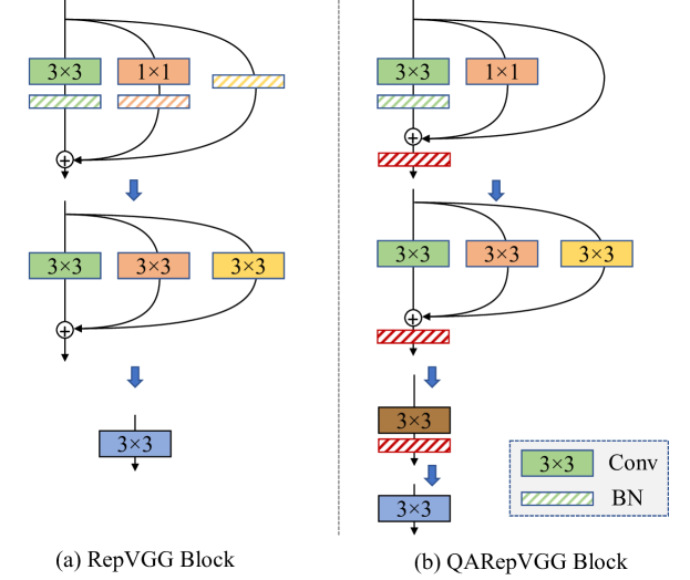
Here, we particularly focus on the quantization difficulty of RepVGG (Ding et al. 2021). To resolve this problem, we explore the fundamental quantization principles that guide us through in-depth analysis of the typical reparameterization-based architecture. That is, for a network to have better quantization performance, the distribution of weights as well as the processed data of an arbitrary distribution shall be quantization friendly. Both are crucial to ensure better quantization performance. More importantly, these principles lead us to a brand new design which we call QARepVGG (short for Quantization-Aware RepVGG) that doesn’t suffer from substantial quantization collapse, whose building block is shown in Fig. 1 and its quantized performance has been largely improved.
Our contributions are threefold,
-
•
Unveiling the root cause of performance collapse in the quantization of the reparameterization-based architecture like RepVGG.
-
•
Contriving a quantization-friendly replacement (i.e. QARepVGG) of RepVGG which holds fundamental differences in terms of weight and activation distribution, meanwhile preserving the very advantage of outstanding speed and performance trade-off.
-
•
Our proposed method generalizes well at different model scales and on various vision tasks, achieving outstanding post-quantization performance that is ready to deploy. Besides, our method has comparable FP32 accuracy as RepVGG and exactly the same fast inference speed under the deploy setting. Therefore, it is a very competitive alternative to RepVGG.
Expectedly, our approach will greatly boost the quantized performance with no extra cost at inference, bridging the gap of the last kilometer during the deployment of reparamenterized networks. We will release the code to facilitate reproduction and future research.
Related Work
Reparameterization Architecture Design. RepVGG (Ding et al. 2021) leverages an over-parameterized network in the form of multiple branches at the training stage and identically fuses branches into one during inference, which is known as reparameterization. This design is becoming wildly used as a basic component in many scenarios, such as edge device application (Vasu et al. 2022; Zhou et al. 2023; Wu, Lee, and Ma 2022; Huang et al. 2022b) , high performance convnet (Ding et al. 2022; Huang et al. 2022a), covering both low-level and high-level vision tasks. Recent popular object detection methods like YOLOv6 (Li et al. 2022) and YOLOv7 (Wang, Bochkovskiy, and Liao 2022) are both built based on such basic component. OREPA (Hu et al. 2022) is a structural improvement on RepVGG, which aims to reduce the huge training overhead by squeezing the complex training-time block into a single convolution. However, almost all these researches make use of the high FP32 performance of reparameterization and fast inference under the deploy setting.
Quantization. Network Quantization is an effective model compression method that maps the network weights and input data into lower precisions (typically 8-bit) for fast calculations, which greatly reduces the model size and computation cost. Without compromising much performance, quantization is mostly adopted to boost speed before deployment, serving as a de facto standard in industrial production. Post-Training Quantization (PTQ) is the most common scheme as it only needs a few batches of images to calibrate the quantization parameters and it comes with no extra training. Quantization-Aware Training (QAT) methods have also been proposed to improve the quantized accuracy, such as integer-arithmetic-only quantization (Jacob et al. 2018), data-free quantization (Nagel et al. 2019), hardware-aware quantization (Wang et al. 2019), mixed precision quantization (Wu et al. 2018), zero-shot quantization (Cai et al. 2020). As QAT typically involves intrusion into the training code and requires extra cost, it is only used when the training code is at hand and PTQ can’t produce a satisfactory result. To best showcase the proposed quantization-aware architecture, we mainly evaluate the quantized accuracy using PTQ. Meanwhile, we include experiments to demonstrate it is also beneficial for QAT.
Quantization for Reparameterization Network. It is known that reparameterization-based architectures have quantization difficulty due to the increased dynamic numerical range due to its intrinsic multi-branch design (Ding et al. 2023). The accuracy degradation of reparameterization models via PTQ is unacceptable. The most related work to ours is RepOpt-VGG, which makes an attempt to address this quantization issue by crafting a two-stage optimization pipeline. However, it requires very careful hyper-parameter tuning to work and more computations. In contrast, our method is neat, robust and computation cheap.
Make Reparameterization Quantization Friendly
This section is organized as follows. First, we disclose that the popular reparameterization design of RepVGG models severely suffers from quantization. Then we make detailed analysis of the root causes for the failure and reveal that two factors incurs this issue: the loss design enlarges the variance of activation and the structural design of RepVGG is prone to producing uncontrolled outlier weights. Lastly, we greatly alleviate the quantization issue by revisiting loss and network design.
Quantization Failure of RepVGG
We first evaluate the performance of several RepVGG models with its officially released code. As shown in Table 1, RepVGG-A0 serevely suffers from large accuracy drop (from 20% to 77% top-1 accuracy) on ImageNet validation data-set after standard PTQ.
A quantization operation for a tensor is generally represented as , where rounds float values to integers using ceiling rounding and truncates those exceed the ranges of the quantized domain. is a scale factor used to map the tensor into a given range, defined as . Where and are a pair of boundary values selected to better represent values distribution of . As shown in (Dehner et al. 2016) and (Sheng et al. 2018), the variance of the quantization error is calculated as . Thus the problem becomes how to reduce the range between and . In practice, they are selected in various ways. Sometimes the maximum and minimum values are used directly, such as weight quantization, and sometimes they are selected by optimizing the MSE or entropy of the quantization error, which is often used to quantify the activation value. The quality of the selection depends on many factors, such as the variance of the tensor, whether there are some outliers, etc.
As for a neural network, there are two main components, weight and activation, that require quantization and may lead to accuracy degradation. Activation also serves as the input of the next layer, so the errors are accumulated and incremented layer by layer. Therefore, good quantization performance for neural networks requires mainly two fundamental conditions:
-
C1
weight distribution is quantization friendly with feasible range,
-
C2
activation distribution (i.e. how the model responds to input features) is also friendly for quantization.
Empirically, we define a distribution of weights or activations as quantization friendly if it has a small variance and few outliers. Violating either one of above conditions will lead to inferior quantization performance.
We use RepVGG-A0 as an example to study why the quantization of the reparameterization-based structure is difficult. We first reproduce the performance of RepVGG with its officially released code, shown in Table 1. Based on this, we can further strictly control the experiment settings. We quantize RepVGG-A0 with a standard setting of PTQ and evaluate the INT8 accuracy, which is dropped from 72.2% to 50.3. Note that we use the deployed model after fusing multi-branches, because the unfused one would incur extra quantization errors. This trick is widely used in popular quantization frameworks.
| Variants | FP32 Acc | INT8 Acc |
|---|---|---|
| (%) | (%) | |
| RepVGG-A0 (w/ custom )⋆ | 72.4 | 52.2 (20.2) |
| RepVGG-A0 (w/ custom )† | 72.2 | 50.3 (21.9) |
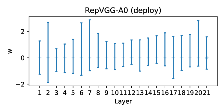
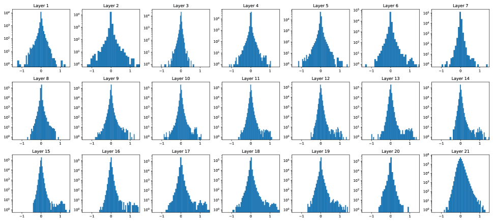
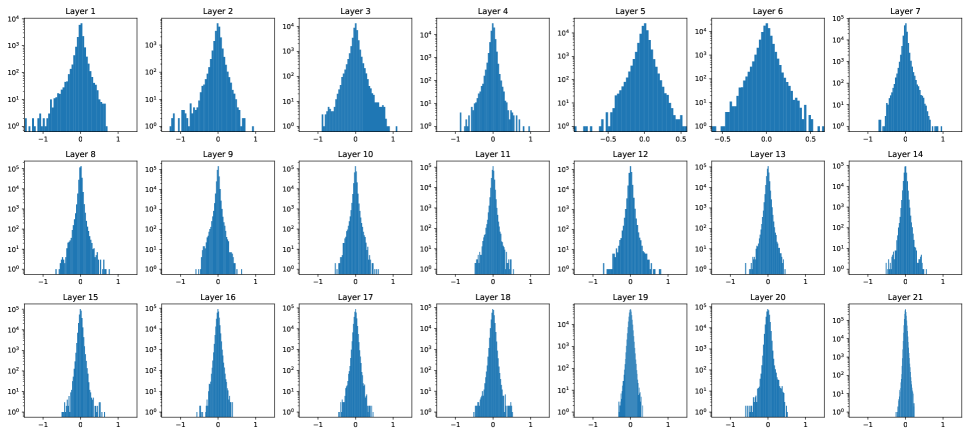
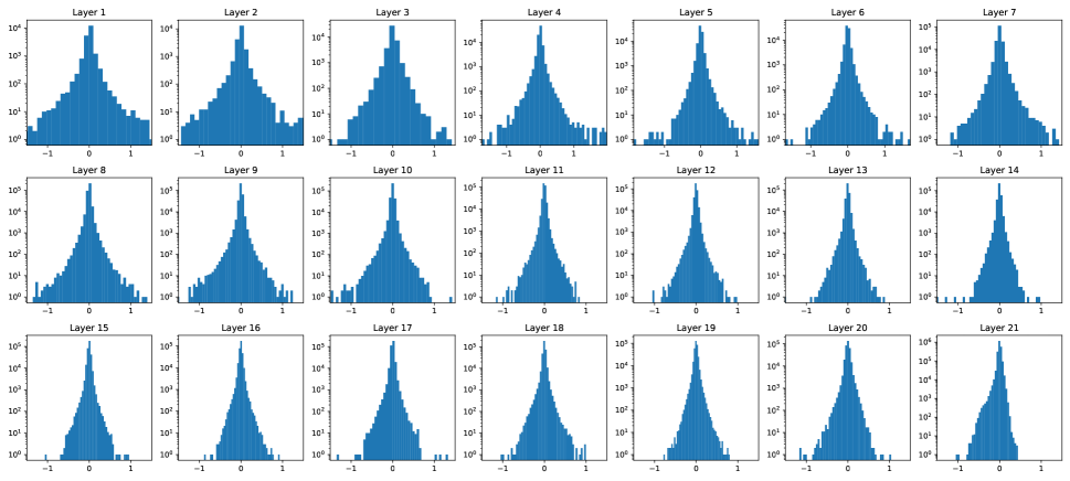
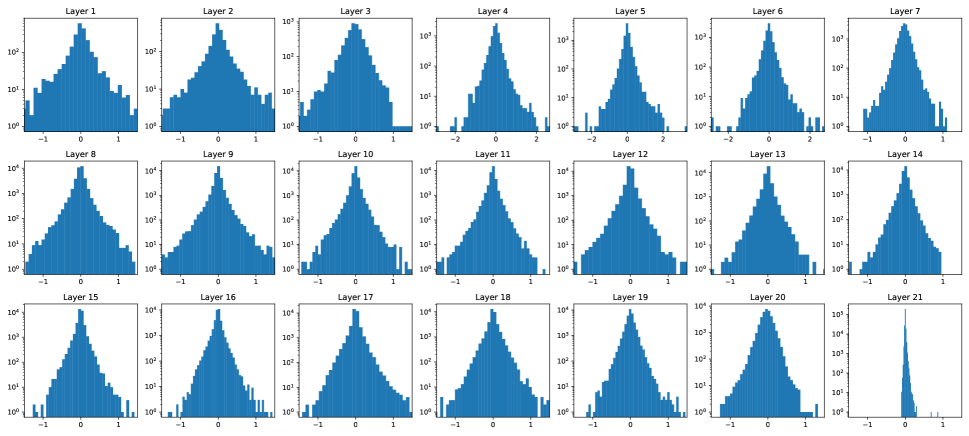
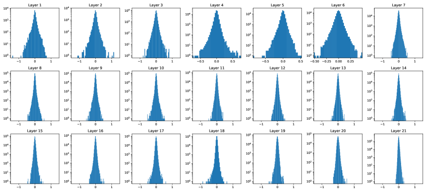
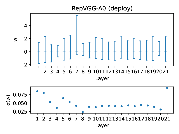
We illustrate the weight distribution of our reproduced model RepVGG-A0 in Fig. 2 and Fig. 13(a) (appendix). Observing that the weights are well distributed around zero and no particular outlier exists, it satisfies C1. This leads us to verify C2 if it is the activation that greatly deteriorates the quantization. Unfortunately, the activation is input-dependent and coupled with the learned weights. We hereby don’t impose any assumptions on the distribution of weight or activation and analyze the deviation of each branch.
Regularized loss enlarges the activation variance
Before we proceed, we formulate the computation operations in a typical RepVGG block. We keep the same naming convention as (Ding et al. 2021) to be better understood. Specifically, we use to denote the kernel of a convolution, where and are the number of input and output channels respectively. Note that for RepVGG. As for the batch normalization (BN) layer after convolution, we use as the mean, standard deviation, scaling factor and the bias. For the BN in the identity branch, we use . Let , be the input and output respectively, and ‘’ be the convolution operator. Let Y,Y and Y be the output of the Identity, 11 and 33 branch. Without loss of generality, we suppose . Then we can write the output as,
| (1) | ||||
The batch normalization operation for the 33 branch can be written as,
| (2) |
where is element-wise multiplication and a small value (10-5 by default) for numerical stability. This means BN plays a role of changing the statistic (mean and variance) of its input. Note that the change of doesn’t affect the quantization error. However, the changed variance directly affects the quantization accuracy. From the probability perspective, given a random variable X, and a scalar , the variance of , i.e. X) equals to (X). Let , then we have
| (3) |
The value of controls shrinking or expanding the variance of , which in turn leads to better or worse quantization performance respectively. For 11 and Identity, we can draw similar conclusions.
Based on the above analysis, we dive into the detail of RepVGG. There is a critical but easily neglected component, which is a special design for the weight decay called custom . It is stated that this component improves the accuracy and facilitates quantization (Ding et al. 2021). The detailed implementation is shown in Algorithm 1 (appendix). This particular design regularizes the multi-branch weights as if it regularizes its equivalently fused kernel. It is likely to make the fused weights enjoy a quantization-friendly distribution111It can be verified by Fig. 13(a) (appendix). . We illustrate the weight distribution of our reproduced model RepVGG-A0 in Fig. 2 and Fig. 13(a) (appendix) and observe that the weights are well distributed around zero and no particular outlier exists.
This loss l2_loss_eq_kernel is essentially,
| (4) |
Notably, the optimizer are encouraged to enlarge the denominator to minimize this loss, which magnifies the variance of activation and brings quantization difficulty. This indicates that custom helps to make learned weights quantization-friendly at the cost of activation quantization-unfriendly. However, we will show that the model have troubles in quantizing learned weights without such regularized loss in the next section and this issue is inevitable because of the structural design.
To address the variance enlarging issue, a simple and straight forward approach is removing the denominator from Eq 4 and we have
| (5) |
We report the result in Table 2. Without the denominator item, the FP32 accuracy is 71.5%, which is 0.7% lower than the baseline. However, it’s surprising to see that the quantization performance is greatly improved to 61.2%. However, this approach still requires inconvenient equivalent conversion.
Another promising approach is applying normal directly. Regarding, previous multi-branch networks like Inception series no longer require special treatment for weight decay, this motivates us to apply normal loss. The result is show in Table 2. Except for simplicity, achieves slightly better result than Eq 5. Therefore, we choose this approach as our default implementation (M1).
| Variants | FP32 Acc | INT8 Acc |
| (%) | (%) | |
| RepVGG-A0 (w/ custom )† | 72.2 | 50.3 (21.9) |
| RepVGG-A0 (Eq 5) | 71.5 | 61.2 (10.3) |
| RepVGG-A0 (w/ normal ) | 71.7 | 61.6 (10.1) |
| QARepVGG-A0 | 72.2 | 70.4 (1.8) |
Structural design of RepVGG is prone to producing uncontrolled outlier weights
While the FP32 accuracy is 0.5% lower than the baseline, its INT8 accuracy is 11.3% higher than the baseline. However, this design doesn’t meet the application requirements either. Given that there are no explicit regularizers to enlarge the activation variance, it is straightforward to check the distribution of weights. Firstly we can give the fused weight as,
| (6) |
where is applied to match shape of the 33 kernel. In this architecture, and are trainable parameters, while is a fixed unit matrix that is not subject to decay during training. The scalars and depend on the outputs of the convolution layers of 33 and 11 branches, respectively. However, directly depends on the output of the last layer. It is worth noting that the Identity branch is special because activations pass through a ReLU layer before entering a BatchNorm layer. This operation can be dangerous since if a single channel is completely unactivated (i.e., contains only zeros), which generate a very small and a singular values of . This issue is common in networks that use ReLU widely. If this case occurs, the singular values will dominate the distribution of the fused kernels and significantly affect their quantization preference.
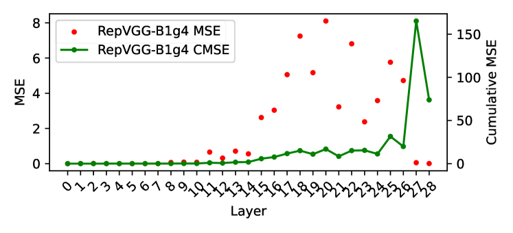
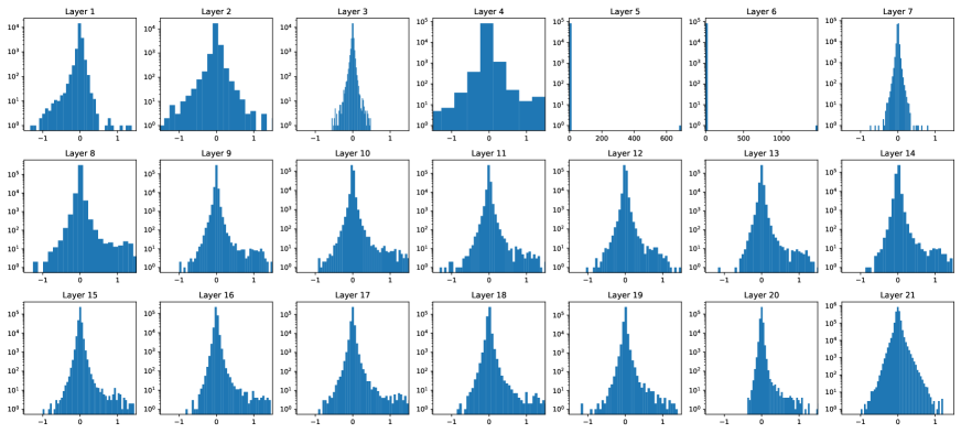
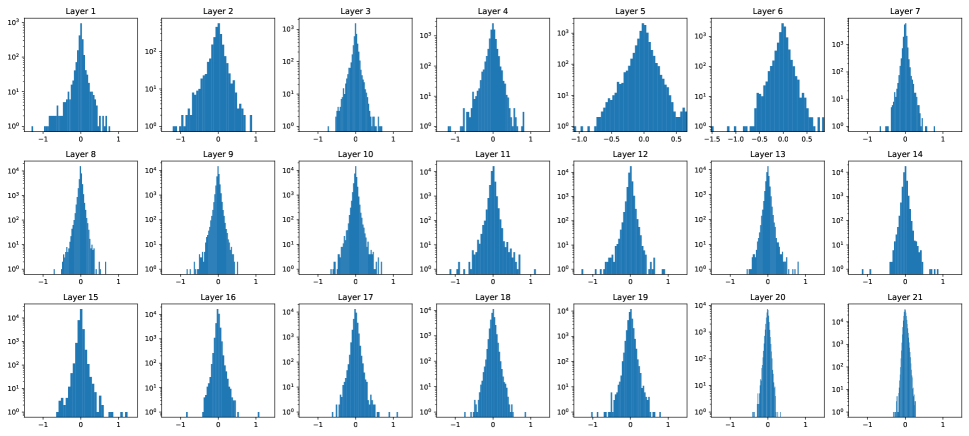
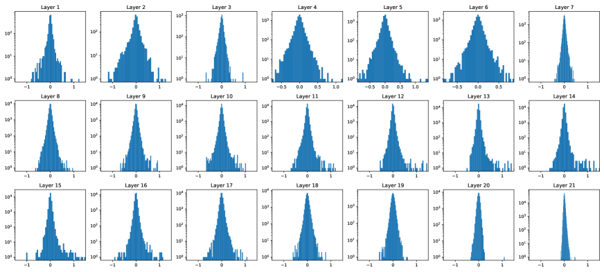
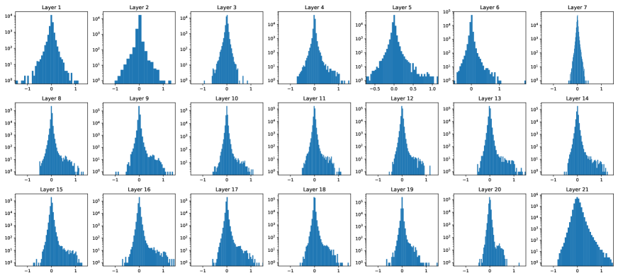
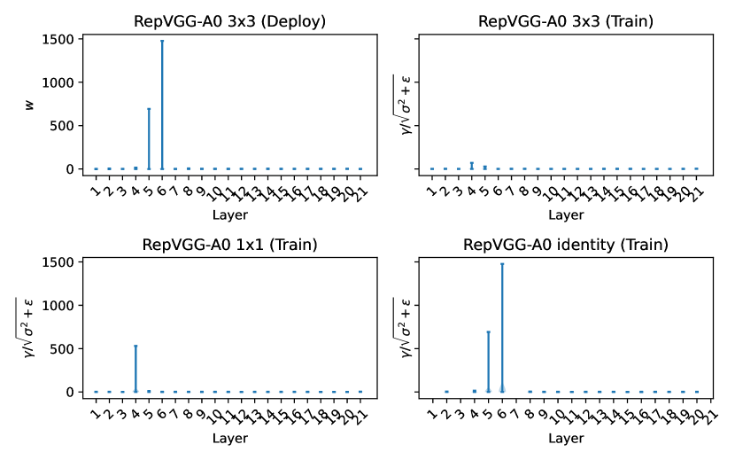
To verify our hypothesis, it is straightforward to check the distribution of weights, which is shown in Fig. 5 (appendix) and Fig. 12 (appendix). The fused weights distribution in both Layer 5 and 6 have large standard variances (2.4 and 5.1 respectively), which are about two orders of magnitude larger than other layers. Specifically, the maximal values of fusedw eights from Layer 5 and 6 are 692.1107 and 1477.3740. This explains why the quantization performance is not good, violating C1 causes unrepairable error. We further illustrate the of three branches in Fig. 5. The maximal values of from the identity branch on Layer 5 and 6 are 692.1107 and 1477.3732. It’s interesting to see that the weights from the 33 and 1 branches from Layer 4 also have some large values but their fused weights no longer contain such values.
We repeat the experiments thrice, and this phenomenon recurs. Note that the maximal values randomly occurs in different layers for different experiments. And simply skip those layers could not solve the quantization problems. Partial quantization results of RepVGG-A0 (w/ custom ) in Table 2 is only 51.3%, after setting Layer 5 and 6 float. According to our analysis, the quantization error for RepVGG is cumulated by all layers, so partial solution won’t mitigate the collapse. This motivates us to address this issue by designing quantization-friendly reparameterization structures.

Quantization-friendly Reparameterization
Based on the normal loss, we solve the above issue by changing the reparameterization structure. Specifically, we remove BN from the identity and 1 branch plus appending an extra BN after the addition of three branches. We name the network based on this basic reparameterization structure QARepVGG. The result is shown in the bottom of Table 2. As for A0 model, QARepVGG-A0 achieves 72.2 top-1 FP32 accuracy and 70.4 INT8 accuracy, which improves RepVGG by a large margin (+20.1%). Next, we elaborate the birth of this design and what role each component plays.
Removing BN from Identity branch (M2) eliminates outlier uncontrolled weights to meet C1.
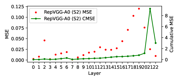
We name this setting S2 and show the result in the third row of Table 3. The error analysis on weight quantization (see Fig. 8 in the appendix) indicates this design indeed meets the requirements of C1 and outlier uncontrolled weight no longer exists. This model delivers a lower FP32 accuracy and INT8 accuracy , which is still infeasible.
The error analysis on weight quantization (see Fig. 8 in the appendix) indicates this design indeed meets the requirements of C1. This model delivers a lower FP32 accuracy and INT8 accuracy , which is still infeasible. This motivates us to verify if it violates C2.
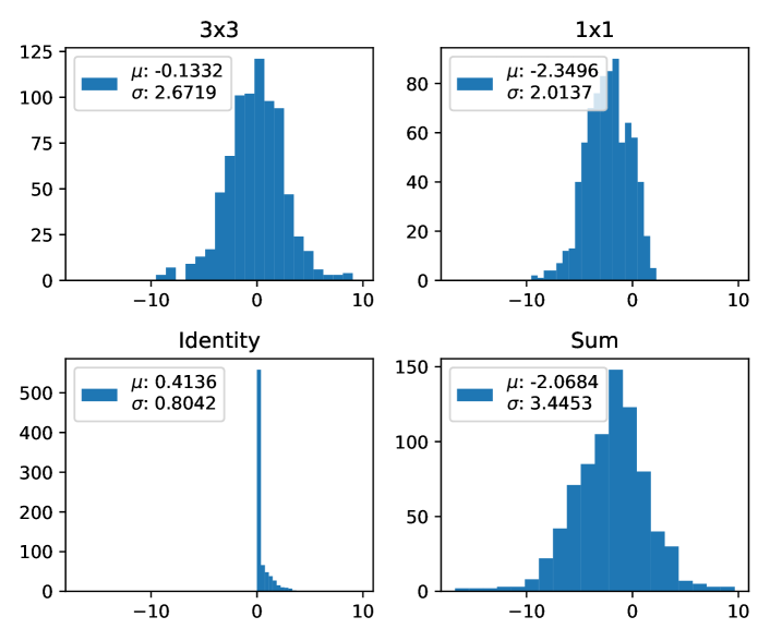
Violating the same mean across several branches shrinks variance of summation to meet C2.
If the and 11 branch have the same mean, their summation is prone to enlarging the variance. This phenomenon occurs frequently under the design of RepVGG. Specifically, ReLU (Nair and Hinton 2010) is the activation function in RepVGG. On one hand, it’s harmful if most inputs are below zero (dead ReLU) (Maas et al. 2013). On the other hand, it’s also not favored if all inputs are above zero because of losing non-linearity. Empirically, many modern high-performance CNN models with BN often have zero means before ReLU. If we take this assumption, we would let . If the and 11 branch have the same mean, we reach . Note , adding three branches often enlarges the variance (Fig. 4). Next, we prove that the original design of RepVGG inevitably falls into this issue as in Lemma 0.1.
| Settings | FP32 Acc (%) | INT8 Acc(%) | |
|---|---|---|---|
| S0 | RepVGG-A0 | 72.2 | 50.3 |
| S1 | +M1 | 71.7 | 61.6 |
| S2 | +M1+M2 | 70.7 | 62.5 |
| S3 | +M1+M2+M3 | 70.1 | 69.5 |
| S4 | +M1+M2+M3+M4 | 72.2 | 70.4 |
| - | +M2 | 70.2 | 62.5 |
| - | +M3 | 70.4 | 69.5 |
| - | +M4 | 72.1 | 57.0 |
We write the expectation of the statistics in three branches as,
| (7) |
Lemma 0.1.
Training a neural network using setting S2 across iterations using loss function , for any given layer, .
The proof is given in the supplementary PDF.
To better control the variance, several simple approaches have potentials, which are shown in Table 4. We choose this design: removing the BN in 11 branch (M3) because it has the best performance. We name this setting S3 and show the result in Table 3. This design achieves 70.1% top-1 FP32 and INT 8 accuracy on ImageNet, which greatly improves the quantization performance. However, its FP32 accuracy is still low.
| Variants | FP32 Acc | INT8 Acc | |
|---|---|---|---|
| (%) | (%) | ||
| 11 wo BN | 70.1 | 69.5 | |
| 33 wo BN | 0.1 | - | |
| 33 wo BN, 11 wo BN | 0.1 | - | |
| 11 with BN (affline=False) | 70.1 | 65.5 |
Extra BN address the co-variate shift issue.
S4 (Post BN on S3)
Since the addition of three branches introduces the covariate shift issue (Ioffe and Szegedy 2015), we append an extra batch normalization after the addition of three branches (M4) to stabilize the training process and name this setting S4 (Fig. 1 right). The post BN doesn’t affect the equivalent kernel fusion for deployment. This further boosts the FP32 accuracy of our A0 model from to on ImageNet. Moreover, its INT8 accuracy is enhanced to .
To summarize, combining the above four modifications together (from M1 to M4) forms our QARepVGG, whose FP32 accuracy is comparable to RepVGG and INT8 performance outperforms RepVGG by a large margin.
Experiment
We mainly focus our experiments on ImageNet dataset (Deng et al. 2009). And we verify the generalization of our method based on a recent popular detector YOLOv6 (Li et al. 2022), which extensively adopts the reparameterization design and semantic segmentation. As for PTQ, we use the Pytorch-Quantization toolkit (NVIDIA 2018), which is widely used in deployment on NVIDIA GPUs. Weights, inputs to convolution layers and full connection layers are all quantized into 8-bit, including the first and last layer. Following the default setting of Pytorch-Quantization toolkit, the quantization scheme is set to symmetric uniform. We use the same settings and the calibration dataset for all the quantization results, except those officially reported ones.
ImageNet Classification
To make fair comparisons, we strictly control the training settings as (Ding et al. 2021). The detailed setting is shown in the appendix. The results are shown in Table 5. Our models achieve comparable FP32 accuracy as RepVGG. Notably, RepVGG severely suffers from quantization, where its INT8 accuracy largely lags behind its FP32 counterpart. For example, the top-1 accuracy of RepVGG-B0 is dropped to 40.2% from 75.1%. In contrast, our method exhibits strong INT8 performance, where the accuracy drops are within 2%.
| Model | FP32 | INT8 | FPS | Params | FLOPs |
| (%) | (%) | (M) | (B) | ||
| RepVGG-A0‡ | 72.4 | 52.2 | 3256 | 8.30 | 1.4 |
| RepVGG-A0† | 72.2 | 50.3 | 3256 | 8.30 | 1.4 |
| QARepVGG-A0 | 72.2 | 70.4 | 3256 | 8.30 | 1.4 |
| RepVGG-B0‡ | 75.1 | 40.2 | 1817 | 14.33 | 3.1 |
| QARepVGG-B0 | 74.8 | 72.9 | 1817 | 14.33 | 3.1 |
| RepVGG-B1g4‡ | 77.6 | 0.55 | 868 | 36.12 | 7.3 |
| QARepVGG-B1g4 | 77.4 | 76.5 | 868 | 36.12 | 7.3 |
| RepVGG-B1g2‡ | 77.8 | 14.5 | 792 | 41.36 | 8.8 |
| QARepVGG-B1g2 | 77.7 | 77.0 | 792 | 41.36 | 8.8 |
| RepVGG-B1‡ | 78.4 | 3.4 | 685 | 51.82 | 11.8 |
| QARepVGG-B1 | 78.0 | 76.4 | 685 | 51.82 | 11.8 |
| RepVGG-B2g4‡ | 78.5 | 13.7 | 581 | 55.77 | 11.3 |
| QARepVGG-B2g4 | 78.4 | 77.7 | 581 | 55.77 | 11.3 |
| RepVGG-B2‡ | 78.8 | 51.3 | 460 | 80.31 | 18.4 |
| QARepVGG-B2 | 79.0 | 77.7 | 460 | 80.31 | 18.4 |
We observe that RepVGG with group convolutions behaves much worse. The accuracy of RepVGG-B2g4 is dropped from 78.5% to 13.7% after PTQ (64.8%). Whereas, our QARepVGG-B2g4 only loses 0.7% accuracy, indicating its robustness to other scales and variants.
Comparison with RepOpt-VGG.
RepOpt-VGG uses gradient reparameterization and it contains two stages: searching the scales and training with the scales obtained. Quantization accuracy can be very sensitive depending on the search quality of scales (Ding et al. 2023).
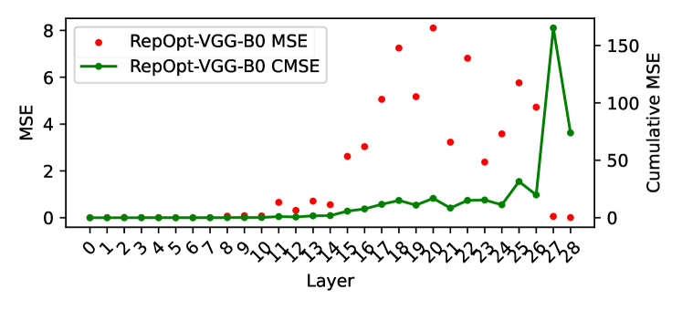
As only a few pre-trained models are released, we retrain RepOpt-VGG-A0/B0 models following (Ding et al. 2023). Namely, we run a hyper-parameter searching for 240 epochs on CIFAR-100 and train for a complete 120 epochs on ImageNet. We can reproduce the result of RepOpt-VGG-B1 with the officially released scales. However, it was hard to find out good scales for A0/B0 to have comparable performance. As shown in Table 6, RepOpt-VGG-A0 achieves 70.3% on ImageNet, which is 2.1% lower than RepVGG. Although being much better than RepVGG, their PTQ accuracies are still too low222 See error analysis for RepOpt-VGG-B0 in Fig. 9 (appendix).. In contrast, our method outperforms RepOpt with clear margins. Besides, we don’t have sensitive hyper-parameters or extra training costs.
| Model | FP32 acc | INT8 acc | Epochs |
|---|---|---|---|
| (%) | (%) | ||
| RepOpt-VGG-A0 | 70.3 | 64.8 (5.5) | 240‡+120 |
| QARepVGG-A0 | 72.2 | 70.4 (1.8) | 120 |
| RepOpt-VGG-B0 | 73.8 | 62.6 (11.2) | 240‡+120 |
| QARepVGG-B0 | 74.8 | 72.9 (1.9) | 120 |
| RepOpt-VGG-B1⋆ | 78.5 | 75.9 (2.6) | 240‡+120 |
| RepOpt-VGG-B1† | 78.3 | 75.9 (2.4) | 240‡+120 |
| QARepVGG-B1 | 78.0 | 76.4 () | 120 |
Comparison using QAT.
We apply QAT from the NVIDIA quantization toolkit on RepVGG, which is de facto standard in practice. The result is shown in Table 7. While QAT significantly boosts the quantization performance of RepVGG, it still struggles to deliver ideal performances because QAT accuracy usually matches FP32. When equipped with QAT, QARepVGG still outperforms RepVGG+QAT by a clear margin. As for QAT comparisons, 1% is recognized as significant improvement. All models are trained for 10 epochs (the first three ones for warm-up) with an initial learning rate of 0.01.
| Model | FP32 (%) | PTQ (%) | QAT (%) |
|---|---|---|---|
| RepVGG-A0 | 72.2 | 50.3 | 66.3 |
| QARepVGG-A0 | 72.2 | 70.4 | 71.9 (5.6) |
| RepVGG-B1g2 | 77.8 | 14.5 | 76.4 |
| QARepVGG-B1g2 | 77.7 | 77.0 | 77.4 (1.0) |
| RepVGG-B2 | 78.8 | 51.3 | 77.4 |
| QARepVGG-B2 | 79.0 | 77.7 | 78.7 (1.3) |
Ablation study on component analysis.
We study the contribution to quantization performance from four modifications and show the results in Table 3. Note that when BN is entirely removed, the model fails to converge. Our design, putting these four components together, is deduced by meeting both C1 and C2 requirements. Single component analysis helps to evaluate which role it plays more quantitatively. It’s interesting that the M3 setting is very near to the VGG-BN-A0 setting (the second row of Table 10), which has lower FP32 and relative higher INT8 accuracy. However, our fully equipped QARepVGG achieves the best FP32 and INT8 accuracy simultaneously.
Object Detection
To further verify the generalization of QARepVGG, we test it on object detectors like YOLOv6 (Li et al. 2022). It extensively makes use of RepVGG blocks and severely suffers from the quantization issue. Although YOLOv6 alleviates this issue by resorting to RepOpt-VGG, the approach is unstable and requires very careful hyperparameter tuning.
We take ‘tiny’ and ‘small’ model variants as comparison benchmarks. We train and evaluate QARepVGG-fashioned YOLOv6 on the COCO 2017 dataset (Lin et al. 2014) and exactly follow its official settings (Li et al. 2022). The results are shown in Table 8. RepVGG and QARepVGG versions are trained for 300 epochs on 8 Tesla-V100 GPUs. RepOpt requires extra 300 epochs to search for scales.
Noticeably, YOLOv6s-RepVGG suffers a huge quantization degradation for about 7.4% mAP via PTQ. YOLOv6t-RepVGG is slightly better, but the reduction of 3% mAP is again unacceptable in practical deployment. Contrarily, YOLOv6s/t-QARepVGG have similar FP32 accuracies to their RepVGG counterpart, while INT8 accuracy drops are restricted within 1.3% mAP. YOLOv6-RepOpt-VGG could give better PTQ accuracy than YOLOv6-RepVGG as well. However, it requires a doubled cost. We also find that the final accuracy of RepOpt-VGG is quite sensitive to the searched hyper-parameters which cannot be robustly obtained.
| Model | FP32 mAP | INT8 mAP | Epochs |
| (%) | (%) | ||
| YOLOv6t-RepVGG | 40.8 | 37.8 (3.0) | 300 |
| YOLOv6t-RepOpt | 40.7 | 39.1 (1.6) | 300+300 |
| YOLOv6t-QARepVGG | 40.7 | 39.5 (1.2) | 300 |
| YOLOv6s-RepVGG⋆ | 42.4 | 35.0 (7.4) | 300 |
| YOLOv6s-RepOpt⋆ | 42.4 | 40.9 (1.5) | 300+300 |
| YOLOv6s-QARepVGG | 42.3 | 41.0 (1.3) | 300 |
Semantic Segmentation
We further evaluate our method on the semantic segmentation task. Specifically, we use two representative frameworks FCN and DeepLabV3+ (Chen et al. 2018) The detailed setting is shown in the supplementary. The results are shown in Table 9. Under the FCN framework, the mIoU is reduced from 72.5% (fp32) to 67.1% (int8) using RepVGG-B1g4. In contrast, mIoU is reduced from 72.6% (fp32) to 71.4% (int8) on top of QARepVGG-B1g4. Under the DeepLabv3+ framework, RepVGG-B1g4 severely suffers from the quantization with 5.3% mIoU drop. Whereas, QARepVGG-B1g4 only drops 1.2%.
| Model | mIoU | mIoU |
|---|---|---|
| FP32(%) | INT8(%) | |
| FCN(RepVGG-B1g4) | 72.5 | 67.1 |
| FCN(QARepVGG-B1g4) | 72.6 | 71.4 |
| DeepLabV3+(RepVGG-B1g4) | 78.4 | 73.1 |
| DeepLabV3+(QARepVGG-B1g4) | 78.4 | 77.2 |
Conclusion
Through theoretical and quantitative analysis, we dissect the well-known quantization failure of the notable reparameterization-based structure RepVGG. Its structural defect inevitably magnifies the quantization error and cumulatively produces inferior results. We refashion its design to have QARepVGG, which generates the weight and activation distributions that are advantageous for quantization. While keeping the good FP32 performance of RepVGG, QARepVGG greatly eases the quantization process for final deployment. We emphasize that quantization awareness in architectural design shall be drawn more attention.
Acknowledgements: This work was supported by National Key R&D Program of China (No. 2022ZD0118700).
References
- Bhalgat et al. (2020) Bhalgat, Y.; Lee, J.; Nagel, M.; Blankevoort, T.; and Kwak, N. 2020. Lsq+: Improving low-bit quantization through learnable offsets and better initialization. In Proceedings of the IEEE/CVF Conference on Computer Vision and Pattern Recognition Workshops, 696–697.
- Cai et al. (2020) Cai, Y.; Yao, Z.; Dong, Z.; Gholami, A.; Mahoney, M. W.; and Keutzer, K. 2020. Zeroq: A novel zero shot quantization framework. In Proceedings of the IEEE/CVF Conference on Computer Vision and Pattern Recognition, 13169–13178.
- Chen et al. (2017) Chen, L.-C.; Papandreou, G.; Kokkinos, I.; Murphy, K.; and Yuille, A. L. 2017. Deeplab: Semantic image segmentation with deep convolutional nets, atrous convolution, and fully connected crfs. IEEE transactions on pattern analysis and machine intelligence, 40(4): 834–848.
- Chen et al. (2018) Chen, L.-C.; Zhu, Y.; Papandreou, G.; Schroff, F.; and Adam, H. 2018. Encoder-Decoder with Atrous Separable Convolution for Semantic Image Segmentation. In ECCV.
- Cordts et al. (2016) Cordts, M.; Omran, M.; Ramos, S.; Rehfeld, T.; Enzweiler, M.; Benenson, R.; Franke, U.; Roth, S.; and Schiele, B. 2016. The cityscapes dataset for semantic urban scene understanding. In Proceedings of the IEEE conference on computer vision and pattern recognition, 3213–3223.
- Dehner et al. (2016) Dehner, G.; Dehner, I.; Rabenstein, R.; Schäfer, M.; and Strobl, C. 2016. Analysis of the quantization error in digital multipliers with small wordlength. In 2016 24th European Signal Processing Conference (EUSIPCO), 1848–1852. IEEE.
- Deng et al. (2009) Deng, J.; Dong, W.; Socher, R.; Li, L.-J.; Li, K.; and Fei-Fei, L. 2009. Imagenet: A large-scale hierarchical image database. In 2009 IEEE conference on computer vision and pattern recognition, 248–255. Ieee.
- Devlin et al. (2019) Devlin, J.; Chang, M.-W.; Lee, K.; and Toutanova, K. 2019. BERT: Pre-training of Deep Bidirectional Transformers for Language Understanding. In Proceedings of the 2019 Conference of the North American Chapter of the Association for Computational Linguistics: Human Language Technologies, Volume 1 (Long and Short Papers), 4171–4186.
- Ding et al. (2023) Ding, X.; Chen, H.; Zhang, X.; Huang, K.; Han, J.; and Ding, G. 2023. Re-parameterizing Your Optimizers rather than Architectures. In The Eleventh International Conference on Learning Representations.
- Ding et al. (2019) Ding, X.; Guo, Y.; Ding, G.; and Han, J. 2019. Acnet: Strengthening the kernel skeletons for powerful cnn via asymmetric convolution blocks. In Proceedings of the IEEE/CVF international conference on computer vision, 1911–1920.
- Ding et al. (2022) Ding, X.; Zhang, X.; Han, J.; and Ding, G. 2022. Scaling up your kernels to 31x31: Revisiting large kernel design in cnns. In Proceedings of the IEEE/CVF Conference on Computer Vision and Pattern Recognition, 11963–11975.
- Ding et al. (2021) Ding, X.; Zhang, X.; Ma, N.; Han, J.; Ding, G.; and Sun, J. 2021. Repvgg: Making vgg-style convnets great again. In Proceedings of the IEEE/CVF Conference on Computer Vision and Pattern Recognition, 13733–13742. https://github.com/DingXiaoH/RepVGG.git, hashtag: 5c2e359a144726b9d14cba1e455bf540eaa54afc.
- Dosovitskiy et al. (2020) Dosovitskiy, A.; Beyer, L.; Kolesnikov, A.; Weissenborn, D.; Zhai, X.; Unterthiner, T.; Dehghani, M.; Minderer, M.; Heigold, G.; Gelly, S.; et al. 2020. An Image is Worth 16x16 Words: Transformers for Image Recognition at Scale. In International Conference on Learning Representations.
- Graves, Mohamed, and Hinton (2013) Graves, A.; Mohamed, A.-r.; and Hinton, G. 2013. Speech recognition with deep recurrent neural networks. In 2013 IEEE international conference on acoustics, speech and signal processing, 6645–6649. Ieee.
- Gupta et al. (2015) Gupta, S.; Agrawal, A.; Gopalakrishnan, K.; and Narayanan, P. 2015. Deep learning with limited numerical precision. In International conference on machine learning, 1737–1746. PMLR.
- Gysel et al. (2018) Gysel, P.; Pimentel, J.; Motamedi, M.; and Ghiasi, S. 2018. Ristretto: A framework for empirical study of resource-efficient inference in convolutional neural networks. IEEE transactions on neural networks and learning systems, 29(11): 5784–5789.
- Habi et al. (2021) Habi, H. V.; Peretz, R.; Cohen, E.; Dikstein, L.; Dror, O.; Diamant, I.; Jennings, R. H.; and Netzer, A. 2021. HPTQ: Hardware-Friendly Post Training Quantization. arXiv preprint arXiv:2109.09113.
- He et al. (2017) He, K.; Gkioxari, G.; Dollár, P.; and Girshick, R. 2017. Mask r-cnn. In Proceedings of the IEEE international conference on computer vision, 2961–2969.
- He et al. (2016) He, K.; Zhang, X.; Ren, S.; and Sun, J. 2016. Deep residual learning for image recognition. In Proceedings of the IEEE conference on computer vision and pattern recognition, 770–778.
- Howard et al. (2019) Howard, A.; Sandler, M.; Chu, G.; Chen, L.-C.; Chen, B.; Tan, M.; Wang, W.; Zhu, Y.; Pang, R.; Vasudevan, V.; et al. 2019. Searching for mobilenetv3. In Proceedings of the IEEE/CVF international conference on computer vision, 1314–1324.
- Howard et al. (2017) Howard, A. G.; Zhu, M.; Chen, B.; Kalenichenko, D.; Wang, W.; Weyand, T.; Andreetto, M.; and Adam, H. 2017. Mobilenets: Efficient convolutional neural networks for mobile vision applications. arXiv preprint arXiv:1704.04861.
- Hu et al. (2022) Hu, M.; Feng, J.; Hua, J.; Lai, B.; Huang, J.; Gong, X.; and Hua, X.-S. 2022. Online Convolutional Re-parameterization. In Proceedings of the IEEE/CVF Conference on Computer Vision and Pattern Recognition, 568–577.
- Huang et al. (2022a) Huang, T.; You, S.; Zhang, B.; Du, Y.; Wang, F.; Qian, C.; and Xu, C. 2022a. DyRep: Bootstrapping Training with Dynamic Re-parameterization. In Proceedings of the IEEE/CVF Conference on Computer Vision and Pattern Recognition, 588–597.
- Huang et al. (2022b) Huang, Z.; Zhang, T.; Heng, W.; Shi, B.; and Zhou, S. 2022b. Real-Time Intermediate Flow Estimation for Video Frame Interpolation. In Proceedings of the European Conference on Computer Vision (ECCV).
- Ignatov et al. (2023) Ignatov, A.; Timofte, R.; Denna, M.; Younes, A.; Gankhuyag, G.; Huh, J.; Kim, M. K.; Yoon, K.; Moon, H.-C.; Lee, S.; et al. 2023. Efficient and accurate quantized image super-resolution on mobile NPUs, mobile AI & AIM 2022 challenge: report. In Computer Vision–ECCV 2022 Workshops: Tel Aviv, Israel, October 23–27, 2022, Proceedings, Part III, 92–129. Springer.
- Ioffe and Szegedy (2015) Ioffe, S.; and Szegedy, C. 2015. Batch normalization: Accelerating deep network training by reducing internal covariate shift. In International conference on machine learning, 448–456. PMLR.
- Jacob et al. (2018) Jacob, B.; Kligys, S.; Chen, B.; Zhu, M.; Tang, M.; Howard, A.; Adam, H.; and Kalenichenko, D. 2018. Quantization and training of neural networks for efficient integer-arithmetic-only inference. In Proceedings of the IEEE conference on computer vision and pattern recognition, 2704–2713.
- Krishnamoorthi (2018) Krishnamoorthi, R. 2018. Quantizing deep convolutional networks for efficient inference: A whitepaper. arXiv preprint arXiv:1806.08342.
- Krizhevsky, Hinton et al. (2009) Krizhevsky, A.; Hinton, G.; et al. 2009. Learning multiple layers of features from tiny images.
- Li et al. (2022) Li, C.; Li, L.; Jiang, H.; Weng, K.; Geng, Y.; Li, L.; Ke, Z.; Li, Q.; Cheng, M.; Nie, W.; Li, Y.; Zhang, B.; Liang, Y.; Zhou, L.; Xu, X.; Chu, X.; Wei, X.; and Wei, X. 2022. YOLOv6: a single-stage object detection framework for industrial applications. arXiv preprint arXiv:2209.02976. https://github.com/meituan/YOLOv6.git, hashtag: 05da1477671017ac2edbb709e09c75854a7b4eb1.
- Lin et al. (2014) Lin, T.-Y.; Maire, M.; Belongie, S.; Hays, J.; Perona, P.; Ramanan, D.; Dollár, P.; and Zitnick, C. L. 2014. Microsoft coco: Common objects in context. In European conference on computer vision, 740–755. Springer.
- Long, Shelhamer, and Darrell (2015) Long, J.; Shelhamer, E.; and Darrell, T. 2015. Fully convolutional networks for semantic segmentation. In Proceedings of the IEEE conference on computer vision and pattern recognition, 3431–3440.
- Maas et al. (2013) Maas, A. L.; Hannun, A. Y.; Ng, A. Y.; et al. 2013. Rectifier nonlinearities improve neural network acoustic models. In ICML, volume 30, 3. Atlanta, Georgia, USA.
- Nagel et al. (2019) Nagel, M.; Baalen, M. v.; Blankevoort, T.; and Welling, M. 2019. Data-free quantization through weight equalization and bias correction. In Proceedings of the IEEE/CVF International Conference on Computer Vision, 1325–1334.
- Nair and Hinton (2010) Nair, V.; and Hinton, G. E. 2010. Rectified linear units improve restricted boltzmann machines. In ICML.
- NVIDIA (2018) NVIDIA. 2018. TensorRT. https://developer.nvidia.com/tensorrt.
- Redmon et al. (2016) Redmon, J.; Divvala, S.; Girshick, R.; and Farhadi, A. 2016. You only look once: Unified, real-time object detection. In Proceedings of the IEEE conference on computer vision and pattern recognition, 779–788.
- Sandler et al. (2018) Sandler, M.; Howard, A.; Zhu, M.; Zhmoginov, A.; and Chen, L.-C. 2018. Mobilenetv2: Inverted residuals and linear bottlenecks. In Proceedings of the IEEE conference on computer vision and pattern recognition, 4510–4520.
- Sheng et al. (2018) Sheng, T.; Feng, C.; Zhuo, S.; Zhang, X.; Shen, L.; and Aleksic, M. 2018. A quantization-friendly separable convolution for mobilenets. In 2018 1st Workshop on Energy Efficient Machine Learning and Cognitive Computing for Embedded Applications (EMC2), 14–18. IEEE.
- Tan and Le (2019) Tan, M.; and Le, Q. 2019. Efficientnet: Rethinking model scaling for convolutional neural networks. In International Conference on Machine Learning, 6105–6114. PMLR.
- Vasu et al. (2022) Vasu, P. K. A.; Gabriel, J.; Zhu, J.; Tuzel, O.; and Ranjan, A. 2022. An Improved One millisecond Mobile Backbone. arXiv preprint arXiv:2206.04040.
- Vaswani et al. (2017) Vaswani, A.; Shazeer, N.; Parmar, N.; Uszkoreit, J.; Jones, L.; Gomez, A. N.; Kaiser, Ł.; and Polosukhin, I. 2017. Attention is all you need. Advances in neural information processing systems, 30.
- Wang, Bochkovskiy, and Liao (2022) Wang, C.-Y.; Bochkovskiy, A.; and Liao, H.-Y. M. 2022. YOLOv7: Trainable bag-of-freebies sets new state-of-the-art for real-time object detectors. arXiv preprint arXiv:2207.02696.
- Wang et al. (2019) Wang, K.; Liu, Z.; Lin, Y.; Lin, J.; and Han, S. 2019. Haq: Hardware-aware automated quantization with mixed precision. In Proceedings of the IEEE/CVF Conference on Computer Vision and Pattern Recognition, 8612–8620.
- Wu et al. (2018) Wu, B.; Wang, Y.; Zhang, P.; Tian, Y.; Vajda, P.; and Keutzer, K. 2018. Mixed precision quantization of convnets via differentiable neural architecture search. arXiv preprint arXiv:1812.00090.
- Wu, Lee, and Ma (2022) Wu, K.; Lee, C.-K.; and Ma, K. 2022. MemSR: Training Memory-efficient Lightweight Model for Image Super-Resolution. In Chaudhuri, K.; Jegelka, S.; Song, L.; Szepesvari, C.; Niu, G.; and Sabato, S., eds., Proceedings of the 39th International Conference on Machine Learning, volume 162 of Proceedings of Machine Learning Research, 24076–24092. PMLR.
- Xu et al. (2022) Xu, S.; Wang, X.; Lv, W.; Chang, Q.; Cui, C.; Deng, K.; Wang, G.; Dang, Q.; Wei, S.; Du, Y.; et al. 2022. PP-YOLOE: An evolved version of YOLO. arXiv preprint arXiv:2203.16250.
- Yun and Wong (2021) Yun, S.; and Wong, A. 2021. Do All MobileNets Quantize Poorly? Gaining Insights into the Effect of Quantization on Depthwise Separable Convolutional Networks Through the Eyes of Multi-scale Distributional Dynamics. In Proceedings of the IEEE/CVF Conference on Computer Vision and Pattern Recognition, 2447–2456.
- Zagoruyko and Komodakis (2017) Zagoruyko, S.; and Komodakis, N. 2017. Diracnets: Training very deep neural networks without skip-connections. arXiv preprint arXiv:1706.00388.
- Zhang, Zeng, and Zhang (2021) Zhang, X.; Zeng, H.; and Zhang, L. 2021. Edge-oriented Convolution Block for Real-time Super Resolution on Mobile Devices. In Proceedings of the 29th ACM International Conference on Multimedia, 4034–4043.
- Zhou et al. (2023) Zhou, S.; Tian, Z.; Chu, X.; Zhang, X.; Zhang, B.; Lu, X.; Feng, C.; Jie, Z.; Chiang, P. Y.; and Ma, L. 2023. FastPillars: A Deployment-friendly Pillar-based 3D Detector. arXiv preprint arXiv:2302.02367.
Appendix A Algorithm
We give the custom implementation in Alg. 1.
Appendix B More Related Work
Quantization-aware architecture design. A quantization-friendly replacement of separable convolution is proposed in (Sheng et al. 2018), where a metric called signal-to-quantization-noise ratio (SQNR) is defined to diagnose the quantization loss of each component of the network. It is also argued that weights shall obey a uniform distribution to facilitate quantization (Sheng et al. 2018). Swish-like activations are known to have quantization collapse which either requires a delicate learnable quantization scheme to recover (Bhalgat et al. 2020), or to be replaced by RELU6 as in EfficientNet-Lite (liu2020higher). BatchQuant (bai2021batchquant) utilizes one-shot neural architecture search for robust mixed-precision models without retraining.
Appendix C Training Setting
ImageNet classfication.
As for model specification, we use the same configuration as (Ding et al. 2021) except for the quantization-friendly reparameterization design, which includes the A and B series. This naturally generates the same deploy model for inference. All models are trained for 120 epochs with a global batch size of 256. We use SGD optimizer with a momentum of 0.9 and a weight decay of . The learning rate is initialized as 0.1 and decayed to zero following a cosine strategy. We also follow the simple data augmentations as (Ding et al. 2021). All experiments are done on 8 Tesla-V100 GPUs.
Semantic segmentation.
We utilize the mmsegmentation (mmseg2020) framework. The hyper-parameters follows the default setting in mmsegmentation. We use SGD with 0.9 momentum and a global batch size of 16. The initial learning rate is 0.1 and decayed to 0.0001 following the polynomial strategy. We use 40k and 80k iterations for FCN and DeepLabv3+ respectively.
Appendix D Discussion
Our method is a structural cure to RepVGG’s quantization difficulty that both works for PTQ and QAT. Though QAT generally delivers better performance, we primarily focus on PTQ since it is more widely used and there is no extra training cost, for this reason we recommended it as the default quantization method. We emphasize that QAT methods can only be applied for RepVGG in deploy mode (single-branch), otherwise directly quantizing multi-branch modules makes them difficult to be fused for higher throughput, where each branch usually has different input ranges and activation distributions. This fact largely limits the feasible QAT performance of RepVGG.
Appendix E More experiments
Error Analysis.
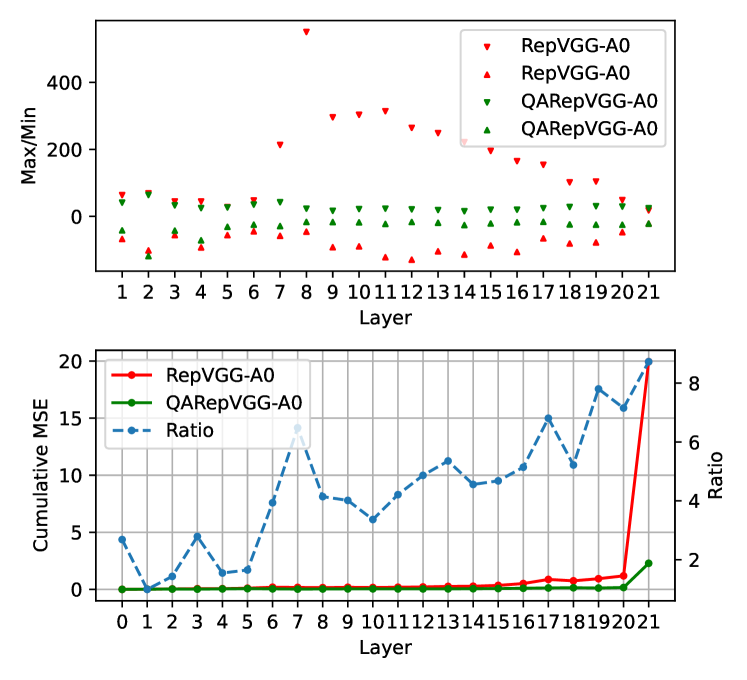
Given that RepVGG-A0 satisfies C1, we sample a batch of images to depict the difference between the two regarding C2 in Fig. 6. Our method produces a better activation distribution of smaller standard variances and min/max values, hence ensuring better quantization performance.
Comparison with VGG (simonyan2015a).
We also product a comparative experiment of vanilla VGG models with the same depth and width. Thus they have the same deployment models. The result is shown in Table 10. QARepVGG outperforms VGG in view of both FP32 and INT8 accuracy.
| Model | FP32(%) | INT8 (%) |
|---|---|---|
| RepVGG-A0 | 72.2 | 50.3 |
| VGG-BN-A0 | 70.4 | 70.1 |
| QARepVGG-A0 | 72.2 | 70.4 |
Comparison with OREPA.
OREPA (Hu et al. 2022) is also a structural improvement on RepVGG. To reduce the training memory, they introduce linear scaling layers to replace the training-time non-linear norm layers, which could maintain optimization diversity and enhance representational capacity. We evaluate the official released models to obtain its PTQ performance, including OREPA-RepVGG-A0, A1 and A2. As shown in Table 11, OREPA could achieve an enjoyable FP32 accuracy, while its PTQ results is far from satisfaction. Particularly, OREPA-RepVGG-A2 suffers an accuracy drop of 13.5% via PTQ. Therefore, such design cannot address the quantization issue of RepVGG.
| Variants | FP32 Acc | INT8 Acc |
|---|---|---|
| (%) | (%) | |
| OREPA-RepVGG-A0 | 73.04 | 63.24 (9.80) |
| OREPA-RepVGG-A1 | 74.85 | 66.35 (8.50) |
| OREPA-RepVGG-A2 | 76.72 | 63.21 (13.51) |
Appendix F Proof
Proof.
We use mathematical induction. Without loss of generality, we use the SGD optimizer. It’s not difficult to check the validity of using other optimizers such as Adam (kingma2014adam).
If , then holds, since they both are initialized by .
Suppose , holds.
When , there is no weight decay for .
| (8) |
Q.E.D. ∎
Appendix G Figures
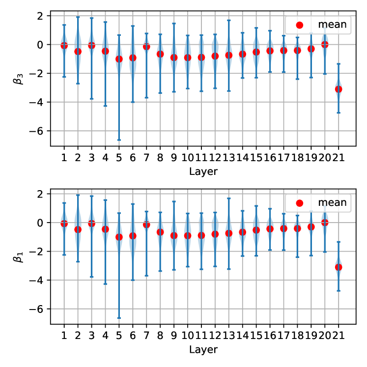
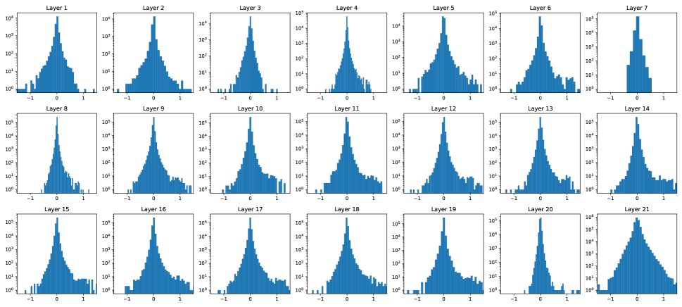
Weight Distribution
Due to built-in weight normalization, either custom L2 or vanilla L2, the convolutional weights generally center around 0 and span unbiasedly for RepVGG-A0, see Figure 13. We also show the violin plot of RepVGG-A0 trained removing the coefficient in in Figure 7. These figures show one of the priors is satisfied to be quantization-friendly.