Multi-resolution Monocular Depth Map Fusion by Self-supervised
Gradient-based Composition

Abstract

Monocular depth estimation is a challenging problem on which deep neural networks have demonstrated great potential. However, depth maps predicted by existing deep models usually lack fine-grained details due to the convolution operations and the down-samplings in networks. We find that increasing input resolution is helpful to preserve more local details while the estimation at low resolution is more accurate globally. Therefore, we propose a novel depth map fusion module to combine the advantages of estimations with multi-resolution inputs. Instead of merging the low- and high-resolution estimations equally, we adopt the core idea of Poisson fusion, trying to implant the gradient domain of high-resolution depth into the low-resolution depth. While classic Poisson fusion requires a fusion mask as supervision, we propose a self-supervised framework based on guided image filtering. We demonstrate that this gradient-based composition performs much better at noisy immunity, compared with the state-of-the-art depth map fusion method. Our lightweight depth fusion is one-shot and runs in real-time, making our method 80X faster than a state-of-the-art depth fusion method. Quantitative evaluations demonstrate that the proposed method can be integrated into many fully convolutional monocular depth estimation backbones with a significant performance boost, leading to state-of-the-art results of detail enhancement on depth maps. Codes are released at https://github.com/yuinsky/gradient-based-depth-map-fusion.

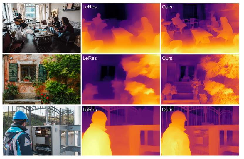
Figure 1: We propose a multi-resolution depth map fusion method to recover high-resolution depth maps. Compared with the single-resolution depth estimation network, the proposed method recovers wide levels of details.

1 Introduction

Depth is an essential information in a wide range of 3D vision applications, bridging 2D images to 3D world. Prior methods of image-based depth estimation rely on multi-view geometry or other scene priors and constraints. In real-life scenarios, multi-view images or additional inputs are not always accessible and monocular depth estimation (depth from a single image) is the most common case. Estimating depth from a single image is a challenging and ill-posed problem, where deep learning demonstrated great potential, by which priors are automatically learnt from training data.

As many other vision tasks based on deep-learning, the predictions of networks are more blurry than the input images, as shown in the second column “$448$” (denotes resolution of $448\times 448$) in Fig. 2. Details are losing due to the down-sampling, max-pooling or convolution operations in the network. Furthermore, although fully convolutional networks take images at arbitrary resolutions as inputs, the networks are overfitted to the fixed resolution of training images. With a testing image at the training resolution, the estimated depth map is more accurate in values. Considering the memory and training time, networks for monocular depth estimation are usually trained in a relatively low resolution. In two most recent monocular depth estimation methods SGR (Xian et al. 2020) and LeRes (Yin et al. 2021), training images are at the resolution of $448\times 448$. Testing images at training low-resolution lead to more accurate depth predictions than those at different resolutions, as demonstrated in Fig. 2. Testing images at original high-resolutions lead to inaccurate predictions of depth values, but keep much more local details. It motivates our explorations in multi-resolution depth map fusion, to combine the depth values and details predicted at different resolutions. It is studied that visual perceptions in natural images include various visual “levels” (Hubel and Wiesel 1962), while different visual “levels” should be considered at the same time to get an overall plausible result.

Instead of treating low- and high-resolution depth predictions equally by symmetry feature encoders, we adopt the core idea of Poisson fusion and propose a novel gradient-based composition network, fusing the gradient domain at high resolution into the depth map at low resolution.

Poisson fusion is not fully differentiable and requires an additional manually labeled mask as input. In order to achieve an end-to-end automatic and differentiable pipeline, we propose a network conceptually inspired by Poisson fusion, without requiring a fusion mask. Based on the observation of higher value accuracy of low-resolution depth, and better texture details of high-resolution depth, we fuse the values of low-resolution depth and gradients of higher-resolution depth by guided filter (He, Sun, and Tang 2010), which is a gradient-preserving filter, to get rid of the requirement of fusion masks. In guided filters, there are two parameters, the window size $r$ is set to adjust the receptive field, along with an edge threshold $\epsilon$.

Here, we fix both parameters for the whole dataset and select high quality data as training set to get a reasonable guided filtered depth map. This depth map is used as the supervision of the gradient domain. By adopting the guided filter in the training phase, our model learn to preserve the detail automatically without the help of guided filters while testing.

In details, the self-supervision is constrained by two separate losses, an image level normalized regression loss (ILNR loss) at the depth domain between the low-resolution depth map and the network prediction, and a novel ranking loss at the gradient domain between guided filtered depth map and the network prediction, as illustrated in Fig. 3. By this self-supervised framework, no labeled data is needed in training.

With most fully convolutional monocular depth estimation methods as backbone, our method effectively enhances their depth maps as in Fig. 1. Details are very well recovered, with the original depth accuracy preserved. Our detailed pipeline is described in Fig. 3. In the depth map fusion network (the gradient-based composition module in Fig. 3), we firstly use a 1-layer convolution to get the approximate gradient map of the depth of higher resolution, then the depth map of lower resolution and the approximated gradient map of high-resolution input are fused in each layer of the 10-layer network to reconstruct the fused depth map. The network structure is designed specifically for a gradient-based composition inspired by Poisson fusion.

Miangoleh et al. (Miangoleh et al. 2021) describe similar observations and adopt GAN to merge low- and high-resolution depth maps of selected patches. Their method (BMD) effectively enhance the details in final depth maps but image noises would confuse their method to decide the high- and low-frequency patches. BMD is also time-consuming with the iterative fashion. Our solutions for multi-resolution depth fusion has a good robustness to image noises, runs in real-time, and fully self-supervised in training. In Sec. 4, we demonstrated that the performance of our method is more stable for different levels of noises, while the state-of-the-art depth map fusion method BMD (Miangoleh et al. 2021) degenerates when the noise variance is high. Our method benefits from the one-shot depth fusion by the lightweight network design, running at 5.4 fps while BMD (Miangoleh et al. 2021) running at 0.07 fps in the same environment. Comprehensive evaluations and a large amount of ablations are conducted, proving the effectiveness of every critical modules in the proposed method.

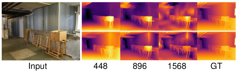
Figure 2: Different input sizes lead to different depth predictions. Low-resolution inputs recover more accurate depth values while higher-resolution inputs lead to more details in depth maps. The numbers denote the actual input sizes to the network after resizing. GT denotes ground truth depth maps. The top row shows depth maps predicted by SGR (Xian et al. 2020) and the bottom row shows depth maps predicted by LeRes (Yin et al. 2021).

Our contributions are summarized as follows:

• A portable network module is proposed to improve fully convolutional monocular depth estimation networks through a multi-resolution gradient-based fusion approach. Our method take advantages of the depth predictions of different resolution inputs, preserving the details while maintaining the overall accuracy.

• A self-supervised framework is introduced to find the optimal fused depth prediction. No labeled data is required.

• The method has good robustness to various image noises, and runs in real-time, while state-of-the-art depth map fusion method degenerates significantly with noises increasing, and takes seconds for each data.

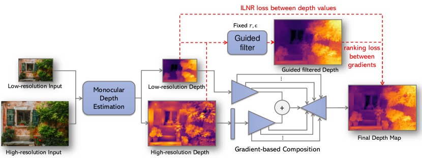
Figure 3: Pipeline of the self-supervised multi-resolution depth map fusion method. With input images at low- and high-resolution, depth maps in two resolutions are predicted by the backbone monocular depth estimation network. The proposed gradient-based composition fuses two depth maps into a plausible one, training in a self-supervised fashion by a ILNR loss in the depth domain and a ranking loss in the gradients domain, supervised by the low-resolution depth map and the guided filtered depth map respectively. The end-to-end pipeline can be integrated with most fully convolutional backbone networks. Red dashed lines denote the procedures included in training phase only.

2 Related work

Monocular depth estimation is an essential step for many 3D vision applications, such as autonomous driving, simultaneous localization and mapping (SLAM (Bailey and Durrant-Whyte 2006)) systems. Estimating depth from one single image is a challenging ill-posed problem, while traditional methods usually require multiple images to explore depth cues. For example, structure from motion (Levinson et al. 2011) is based on the feature correspondences among multi-view images. With only one image, it is infeasible to solve the ambiguities.

For ill-posed problems, deep neural networks show a good superiority. Deep-learning based methods can be categorized by supervision styles. A most straight-forward solution is supervised learning. Eigen et al. (Eigen, Puhrsch, and Fergus 2014) proposes the first supervised work to solve monocular depth estimation, by defining Euclidean losses between predictions and ground truths to train a two-component network (global and local network). Mayer et al. (Mayer et al. 2016) solves scene flow in a supervised manner. Monocular depth estimation, along with optical flow estimation, are working as sub-problems of scene flow estimation. Recently, pretrained layers in ResNet (He et al. 2016) are widely used in monocular depth estimation networks (Xian et al. 2018; Ranftl et al. 2019; Yin et al. 2021) to speed up the training. Semi-supervised methods (Smolyanskiy, Kamenev, and Birchfield 2018; Kuznietsov, Stuckler, and Leibe 2017; Amiri, Loo, and Zhang 2019) training from stereo pairs are proposed to soften the requirement of direct supervision. They estimate disparity between two stereo images, and define a consistency between one input image, and the re-rendered image by estimated inverse depth, disparity, camera pose and the other input. Kuznietsov et al. (Kuznietsov, Stuckler, and Leibe 2017) use sparse supervision from LIDAR data and incorporate with berHu norm (Zwald and Lambert-Lacroix 2012). Following works based on LIDAR data (He et al. 2018; Wu et al. 2019) propose similar semi-supervised training pipelines. Unsupervised methods (Godard et al. 2019; Casser et al. 2019; Bozorgtabar et al. 2019; Zhu et al. 2018) are mostly relying on the constraint of re-projections between neighboring frames in their training image sequences. By getting rid of supervisions, these methods suffer from many problems such as scale ambiguities and scale inconsistencies. Other than different supervisions, different losses or constraints are adopted to better constrain the problem. Methods based on Berhu loss (Heise et al. 2013; Zhang et al. 2018), conditional random fields (Li et al. 2015; Liu et al. 2015; Wang et al. 2015) or generative adversarial networks (GAN) (Feng and Gu 2019; Jung et al. 2017; Gwn Lore et al. 2018) are proposed.

A common issue of deep-learning methods is that many depth details are lost in network outputs. Depth maps are usually blurry with inaccurate details such as planes and object boundaries. This issue exists in many vision problems, such as image segmentation and edge detection. Deep-learning methods generate results much more blurry than non-CNN methods. Although replacing input images of higher resolutions generate predictions with higher resolutions, it leads to inaccurate depth values, as shown in Figure 2. It motivates our work to fuse the depth maps of different resolutions to get an overall plausible one. Traditional image fusion methods such as Poisson fusion (Pérez, Gangnet, and Blake 2003), Alpha blending (Porter and Duff 1984) require additional inputs such as alpha weights or masks, which usually require manual labeling. The proposed method automatically decides which regions from two-resolution depth maps have to be fused and how to fuse them. A recent depth map fusion method (Miangoleh et al. 2021) uses GAN to fuse the low- and high-resolution depths. Our method solves two-resolution depth fusion by self-supervised gradient-domain composition, achieving better robustness on image noises and real-time performance.

3 Method

3.1 Overview

Our key observation for monocular depth map fusion is that the local details can be preserved in the gradient domain of depth estimation from a high-resolution input, while the global value accuracy is better estimated with low-resolution input. In other words, a convolutional neural network (CNN) can focus on different levels of details when dealing with input images of different resolutions. Therefore, fusing the predictions of multi-resolution inputs is a straightforward choice to enhance the depth estimation. The goal of our method is finding the optimal fusion operation $\oplus$ for $d_{\text{high}}$ and $d_{\text{low}}$, which are depth predictions of the input image $I$ at high- and low-resolutions:

$$f=d_{\text{high}}\oplus d_{\text{low}},$$ (1)

where $f$ is the fused depth estimation with enhanced details.

Inspired by the Poisson fusion, the fusion operation $\oplus$ should transplant the gradient domain of $d_{\text{high}}$ to $d_{\text{low}}$ for detail-preserving. Thus, we formulate the optimization of depth fusion as below,

$$\min_{\oplus}\iint_{\Omega}|\triangledown f-\triangledown d_{\text{high}}|\partial\Omega+\iint_{I-\Omega}|f-d_{\text{low}}|\partial\Omega,$$ (2)

where $\triangledown$ denotes the gradients of an image. Note that the optimization of $\oplus$ only focus on the gradient domain within $\Omega$ and value domain among other areas $I-\Omega$, where $\Omega$ is the area $d_{\text{high}}$ has better details than $d_{\text{low}}$. We propose a self-supervised neural network to find the fusion operation $\oplus$ based on Eq. 2.

Note that the classic Poisson fusion is not differentiable while calculating the fused gradient around boundaries of fusion area $\Omega$. We first introduce a multi-level gradient-based fusion network module to approximate the Poisson fusion, which is described in Sec. 3.2. Since we have no supervision of $\Omega$ to train this fusion module, we propose a self-supervised framework based on the supervision of guided filtering with a novel training loss, and details are in Sec. 3.3. Therefore, the fusion module in our pipeline is fully differentiable and capable of preserving gradient details of proper fusion area $\Omega$ while maintaining overall consistency and the training is fully self-supervised. Implementation details are provided in Sec. A.2. At last, the evaluations Sec. 4 demonstrates the superiority of the method on depth estimation accuracy and detail preservation over the state-of-the-art alternatives with better efficiency, and robustness to image noises and complicated textures.

3.2 Multi-level gradient-based depth fusion

Monocular depth estimation. Our multi-level gradient-based depth fusion module requires monocular depth estimation with different resolutions as inputs. LeRes(Yin et al. 2021) is a novel and state-of-the-art monocular depth estimation network that can provide good depth initials. However, it also lacks the capacity of providing clear depth details. We adopt LeRes(Yin et al. 2021) as the backbone to produce the depth initialization with different resolutions for depth fusion. As shown in Fig. 2, the prediction of images with higher resolution contains more details while the lower resolution image can achieve higher overall accuracy. For each input $I$, we adopt two different resolutions $I_{\text{low}},I_{\text{high}}$ for the fusion operation, the corresponding predictions are $d_{\text{low}},d_{\text{high}}$ respectively.

Note that our method can also work with other monocular depth estimation backbones. The evaluations with other three monocular single-resolution methods (Xian et al. 2020; Yuan et al. 2022; Ranftl, Bochkovskiy, and Koltun 2021) as backbone methods are provided in Sec. 4.

Differentiable gradient-domain composition. Poisson fusion could be a good candidate for constructing the depth fusion module since it takes the gradient consistency into optimization. To ensure that the whole framework of our method can be trained in an end-to-end manner, we need to find a differentiable approximation to deal with the truncation of gradient backward around the merging boundaries.

To avoid the gradient truncation, we adopt an encoder-decoder framework to formulate the fusion module which can utilize $\Omega$ implicitly in the latent space. Then we can rewrite Eq. 1 as below:

$$f=\mathcal{D}(\mathcal{E}_{l}(d_{\text{low}})+\mathcal{E}_{h}(d_{\text{high}}),\Omega)$$ (3)

where $\mathcal{D}$ is the decoder module, and $\mathcal{E}_{l}$, $\mathcal{E}_{h}$ are the encoder modules for low- and high-resolution depth estimations.

However, this formulation has two problems in implementation. First, $\Omega$ requires supervision but there are no such datasets. Thus, a self-supervised framework is proposed to solve this problem in Sec. 3.3. Second, training an encoder-decoder framework is highly inefficient if $\mathcal{E}_{l}$ and $\mathcal{E}_{h}$ do not share hyperparameters, however, sharing all hyperparameters will degrade the performance. Since we want to extract gradient information from $d_{\text{high}}$ and the depth values from $d_{\text{low}}$, it is natural to formulate $\mathcal{E}_{h}$ based on $\mathcal{E}_{l}$ with an additional one-level convolution layer $\mathcal{E}_{g}$ to extract gradients.

$$\mathcal{E}_{h}(\cdot)=\mathcal{E}_{l}(\mathcal{E}_{g}(\cdot))$$ (4)

$\mathcal{E}_{g}(d_{\text{high}})$ can be considered as a varied approximation with tunable parameters of $\triangledown d_{high}$. Therefore, Eq. 3 can be rewritten as,

$$f=\mathcal{D}(\mathcal{E}_{l}(d_{\text{low}})+\mathcal{E}_{l}(\mathcal{E}_{g}(d_{\text{high}})),\Omega)$$ (5)

This solution is simple yet effective. Sharing most hyperparameters between $\mathcal{E}_{l}$ and $\mathcal{E}_{h}$ is highly efficient in the training stage. Our evaluation also demonstrates that the fusion performance will drop significantly if $\mathcal{E}_{g}$ is absent in the Eq. 5, which means this design is critical and essential. A visual comparison upon $\mathcal{E}_{g}$ is presented in Fig. 4 which support our claimant as well.

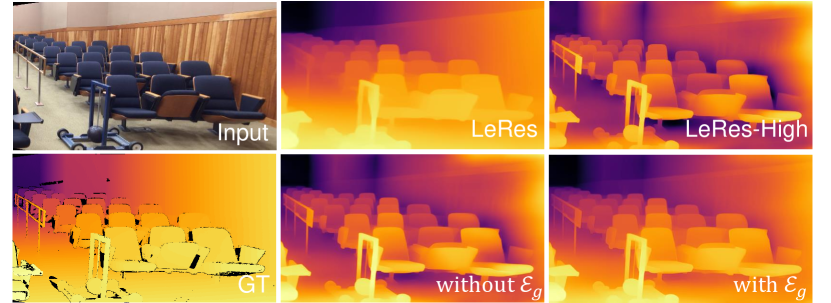
Figure 4: Visual comparison upon $\mathcal{E}_{g}$. LeRes and LeRes-High are depth estimation results given by LeRes(Yin et al. 2021) with low- and high resolution inputs.

Multi-level fusion framework. To fully utilize $d_{\text{low}}$ and $d_{\text{high}}$ with neural networks, a simple one-step fusion with Eq. 5 is not enough. A pyramid-style framework is introduced to fuse depth at different resolutions. We formulate Eq. 5 with the multi-level encoder $\mathcal{E}^{2^{i}}_{l}$ as below:

$$f=\mathcal{D}(\sum_{i=2}^{11}\mathcal{E}^{2^{i}}_{l}(d_{\text{low}})+\mathcal{E}^{2^{i}}_{l}(\mathcal{E}_{g}(d_{\text{high}})),\Omega)$$ (6)

where $\mathcal{E}^{2^{i}}_{l}$ is multi-layer fully convolution module with resolution $2^{i}$. For implementation of Eq. 6, we take $d_{\text{low}}$ and $\mathcal{E}_{g}(d_{\text{high}})$ into a multi-level convolution-based encoder individually. The convoluted outputs of $d_{\text{low}}$ and $\mathcal{E}_{g}(d_{\text{high}})$ from each level are then skip connected and be supplied as input for layered upsampling and convolution modules to reconstruct the final depth map.

3.3 Self-supervised framework of depth fusion

Self-supervision with guided filtering. Image fusion based on Poisson equations introduces us to an interesting idea to fuse predictions of different resolution images. However, the classic Poissons-based fusion requires the manual labeling of the fusion area $\Omega$. To get rid of the manual steps we still need a proper $\Omega$ for depth fusion, training under the supervision of existing datasets is the most straightforward way. Unfortunately, no datasets are available for providing such information. We introduce a self-supervision mechanism driven by guided filtering to deal with this problem.

The guided filtering is an edge-preserving filtering, it has the gradient smoothing property. This filter fuses $d_{\text{low}}$ and $d_{\text{high}}$ together while keeping the gradient details of $d_{\text{high}}$ without manual mask labels like $\Omega$. This character makes it a perfect supervision for training our network. However, the guided filtering requires additional parameters to control fusion quality, and the tunable parameters are data dependent. Fortunately, we find that in the gradient domain of the fused image, a preset parameter works for the training set. Therefore, we can rewrite Eq. 2 as below,

$$\min_{\oplus}\iint|\triangledown f-\triangledown d_{\text{gf}}|+|f-d_{\text{low}}|\partial\Omega,$$ (7)

where $d_{\text{gf}}$ is the fused result of $d_{\text{low}}$ and $d_{\text{high}}$ through guided filtering with a set of fixed parameters. The ablations in Section 4 demonstrate that $d_{\text{gf}}$ provide effective supervision for training $\oplus$. Our fused module outperforms guided filtering as well in evaluations.

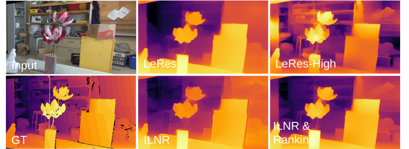
Figure 5: Visual comparison upon $l_{\text{mILNR}}$ and $l_{\text{rank}}$. LeRes and LeRes-High are depth results by LeRes(Yin et al. 2021) with low- and high-resolution inputs. ILNR is the fused result training only by $l_{\text{mILNR}}$ while ours adopts both.

Self-supervised loss. The training objective Eq. 7 is then optimized through the self-supervised loss $l_{\text{fusion}}$ as below,

$$l_{\text{fusion}}(f,d_{\text{gf}},d_{\text{low}})=l_{\text{mILNR}}(f,d_{\text{low}})+l_{\text{rank}}(f,d_{\text{gf}}),$$ (8)

where $l_{\text{mILNR}}=\sum_{r}l_{\text{ILNR}}(f^{r},d^{r}_{\text{low}})$ is multi-resolution image-level normalized regression (ILNR) loss (Yin et al. 2021) which constrains the value domain of fused result $f$ to be similar as $d_{\text{low}}$ at every resolution $r$ levels. Another term $l_{\text{rank}}$ is a novel ranking loss inspired by (Xian et al. 2020) which constrains the gradient domain of $f$ being close to $d_{\text{gf}}$. Given a pair of points $i,j$, ${p^{i}_{f}\in f,p^{i}_{\text{gf}}\in d_{\text{gf}}}$ are pixels on $f$ and $d_{\text{gf}}$ respectively. $l_{\text{rank}}=\frac{1}{N}\sum_{i,j}E(p^{i}_{f},p^{j}_{f},p^{i}_{\text{gf}},p^{j}_{\text{gf}})$ is formulated based on these sampled pixel pairs, and $N$ is the number of pixel pairs. Point pair $i,j$ are sampled based on edge areas $M$ extracted from $\triangledown d_{\text{gf}}$ and $\triangledown d_{\text{high}}$ by Canny detection.

where $z_{ij}$ is an indicator, $z_{ij}=1$ means pixel $i,j$ are located on different sides of an edge of $M$ while $z_{ij}=0$ means they located on the same side. $\sigma$ is a regular term for robust compuatation. A visual comparison upon our loss terms $l_{\text{mILNR}}$ and $l_{\text{rank}}$ is presented in Fig. 5, which demonstrate the our design of losses is effective.

4 Experiments

Methods	Multiscopic					Middlebury2021					Hypersim
	SqRel$\downarrow$	rms$\downarrow$	log10$\downarrow$	$\delta_{1}\uparrow$	$\delta_{2}\uparrow$	SqRel$\downarrow$	rms$\downarrow$	log10$\downarrow$	$\delta_{1}\uparrow$	$\delta_{2}\uparrow$	SqRel$\downarrow$	rms$\downarrow$	log10$\downarrow$	$\delta_{1}\uparrow$	$\delta_{2}\uparrow$
SGR	9.161	14.031	0.086	0.745	0.904	0.846	3.948	0.067	0.773	0.94	0.593	1.536	0.102	0.612	0.854
NeWCRFs	11.031	14.658	0.088	0.749	0.899	0.829	3.724	0.058	0.830	0.952	0.513	1.322	0.088	0.694	0.881
DPT	4.021	9.781	0.059	0.841	0.904	0.700	3.698	0.060	0.827	0.956	0.327	1.145	0.083	0.734	0.914
LeRes	9.168	13.12	0.082	0.776	0.909	0.464	3.042	0.052	0.847	0.969	0.319	1.011	0.071	0.768	0.924
SGR-GF	9.314	14.107	0.087	0.743	0.903	0.844	3.9	0.067	0.773	0.94	0.600	1.539	0.103	0.612	0.854
NeWCRFs-GF	10.601	14.407	0.087	0.751	0.901	0.796	3.549	0.058	0.832	0.953	0.518	1.320	0.088	0.694	0.881
DPT-GF	4.142	10.060	0.060	0.835	0.935	0.685	3.653	0.060	0.825	0.956	0.332	1.149	0.083	0.733	0.914
LeRes-GF	9.01	13.063	0.082	0.776	0.91	0.457	2.976	0.052	0.849	0.968	0.324	1.011	0.072	0.769	0.922
3DK	9.379	14.879	0.077	0.73	0.895	0.911	4.18	0.069	0.745	0.945	0.718	1.521	0.108	0.610	0.840
LeRes-BMD	9.259	13.101	0.083	0.773	0.91	0.487	3.014	0.055	0.844	0.96	0.312	0.993	0.072	0.769	0.922
SGR-Ours	9.144	14.0	0.086	0.746	0.905	0.816	3.858	0.067	0.776	0.942	0.605	1.549	0.103	0.609	0.851
NeWCRFs-Ours	10.405	14.299	0.087	0.752	0.902	0.786	3.587	0.057	0.832	0.953	0.520	1.324	0.089	0.687	0.880
DPT-Ours	3.998	9.759	0.058	0.841	0.938	0.647	3.533	0.059	0.832	0.958	0.311	1.109	0.081	0.745	0.915
LeRes-Ours	8.833	12.921	0.081	0.781	0.911	0.444	2.963	0.051	0.853	0.969	0.315	0.999	0.071	0.77	0.923

Table 1: The quantitative evaluations on three benchmark datasets. Bold numbers denote the best result while underlined numbers are second best. Depth map fusion methods on monocular depth estimation backbones are presented as “backbone-fusion method”. Our method achieve the best performance on $13/15$ metrics in these 3 datasets.

In Sec. 4.1, we introduce the benchmark datasets used in evaluations. In Sec. 4.2, we compare the proposed method with several state-of-the-art monocular depth estimation methods and depth refinement methods in aspects of several error metrics, robustness to noises, and running time. Lastly, in Sec. 4.3, we conduct several ablations to study the effectiveness of several critical design in the proposed pipeline.

4.1 Benchmark datasets and evaluation metrics

To evaluate the depth estimation ability of our method, we adopt several commonly used zero-shot datasets, which are Multiscopic (Yuan et al. 2021), Middlebury2021 (Scharstein et al. 2014) and Hypersim (Roberts et al. 2021). All benchmark datasets are unseen during training.

In evaluations, we test on the whole set of Middlebury2021 (Scharstein et al. 2014), including 24 real scenes. For Multiscopic (Yuan et al. 2021) dataset, we evaluate on synthetic test data, containing 100 high resolution indoor scenes. For Hypersim (Roberts et al. 2021), we evaluate on three subsets of 286 tone-mapped images generated by the released codes. On these datasets, we evaluate several error metrics. $SqRel$ and $rms$ denote two common metrics, which are the square relative error and the root mean square error, respectively. The mean absolute logarithmic error $log_{10}$ is defined as $log_{10}=\frac{1}{N}\sum{\left\|log(d_{i}^{*})-log(d_{i})\right\|}$. The error metric $delta$ describes the percentage of pixels satisfying $\delta=max(\frac{d_{i}^{*}}{d_{i}},\frac{d_{i}}{d_{i}^{*}})<1.25^{k}$ (i.e. $\delta_{1.25}^{k}$), $k=1,2$ are adopted to evaluate our performance, which are $\delta_{1},\delta_{2}$ in the tables. $D^{3}R$ metric measures the detected edge error, which is introduced in (Miangoleh et al. 2021). In all metrics $d_{i}^{*}$ is the ground truth depth value and $d_{i}$ denote the predict value at pixel $i$. Due to the scale ambiguity in monocular depth estimation, we follow Ranftl et al. (2019) to align the scale and shift using the least squares before computing errors.

4.2 Comparisons to state-of-the-arts

Quantitative Evaluation. We compare our method with two state-of-the-art fusion based monocular depth estimation alternatives, BMD (Miangoleh et al. 2021), and 3DK (Niklaus et al. 2019), in Tab. 1. To demonstrate that our self-supervised framework is effective, we also present the performance of monocular depth estimation methods applying with guided filter (He, Sun, and Tang 2010) as a baseline. In the comparison, we adopt the trained models released by the authors and evaluate with their default configuration.

Tab. 1 demonstrate that our method outperform all the other fusion based depth estimation alternatives on most benchmarks and error metrics. Our method also produce better fusion results than guided filtering which is our training supervision. It means that our network takes advantages of both the low-resolution input and the guided filtered fusion result but not strictly constrained. It should be noticed that our method was trained with the monocular depth estimation backbone LeRes (Yin et al. 2021). The trained fusion module can be directly integrated with other fully convolutional monocular depth estimation networks such as SGR (Xian et al. 2020), NeWCRFs (Yuan et al. 2022) and DPT (Ranftl, Bochkovskiy, and Koltun 2021), without any fine-tuning. The proposed method is portable and can be easily incorporated into many state-of-the-art depth estimation models.

We also evaluate the details recovered by our method. We present the comparison between our method and two backbone methods with $D^{3}R$ metric in Tab. 2, which measure the edge correctness of the estimation depth details.

Method	Multiscopic	Middlebury2021
SGR	0.576	0.735
DPT	0.594	0.613
NeWCRFs	0.767	0.737
LeRes	0.570	0.719
Ours	0.542	0.589

Table 2: Evaluation of our fusion module on edge correctness of depth by $D^{3}R$ metric, where lower values are better.

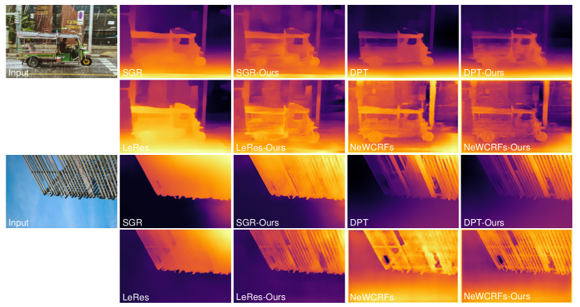
Figure 6: Qualitative comparisons on unseen natural images from the Internet. Our method successfully boosts the performances of the backbone monocular depth estimation methods, and recovers the details in depth maps.

Visual Comparisons. The qualitative evaluations are presented in Fig. 6. As discussed earlier, most monocular depth estimation methods suffer from blurry predictions. The improvement of detail-preserving by our multi-resolution depth map fusion is significant. Most details missing in the backbone methods are successfully recovered, while keeping the original depth values correct. Additional examples are shown in Fig. 17-20, our fusion method can significantly improve performance of SGR (Xian et al. 2020) and LeRes (Yin et al. 2021).

Anti-noise Evaluation. One of the main advantages of our method over the state-of-the-art depth fusion method BMD (Miangoleh et al. 2021) is the noise robustness enabled by our gradient-based fusion. Since BMD determines fusion areas explicitly by edge detection, its performance will drop significantly while the input images include noises. We compare the anti-noise ability of our methods with BMD. For evaluation, we add Gaussian noises or Pepper noises to the input image. The mean value of Gaussian noises is 0, the variances changes from 0.001 to 0.009 for Gaussian noises, and the signal-noise ratio changes from $100\%$ to $95\%$ for Pepper noises. Fig. 8 shows the variety of $\delta_{1}$ value when adopting different variance levels of Gaussian (left) or Pepper noises (right). Fig. 15 also presents visual examples of our method comparing with BMD, on input images with two types of noises.

Fusion based methods such as BMD can also be easily influenced by the complicated textures. We split Middlebury2021 benchmark into two sub-sets based on the edge number detected in the ground truth depth images. Less edges on depth maps means more depth independent textures exist. The plot at the left of Fig. 7 demonstrates that our method outperforms BMD more significantly on the difficult sub-set. At the right of Fig. 7, a visual comparison on a difficult example is shown, where BMD suffers from the complicated textures and extract many texture details into the depth map (e.g. paintings on the whiteboard).

Running time. Our fusion module is one-shot and requires no additional complex processing, it is highly efficient and only takes $68\%$ processing time comparing with LeRes for depth estimation of high resolution input. The fusion processing of our method is 10X faster than guided filter while present better performance. The whole pipeline of our method, including the depth estimation time of low- and high-resolution inputs, is more than 80X faster than BMD. Detailed time and computational statistics can be found in Tab. 7.

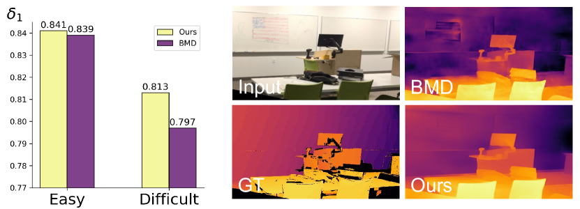
Figure 7: Left: Quantitative evaluation between our method and BMD on easy and difficult datasets regarding to texture complexities. Ours outperform BMD more significantly on the difficult subset. Right: Visual comparisons between our method and BMD.

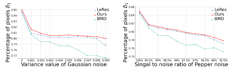
Figure 8: Quantitative evaluation of anti-noise ability of LeRes, BMD and ours. The vertical axis denotes the value of $\delta_{1.25}$, which is the higher the better.

4.3 Ablation studies

	Loss function				Result
	ILNR	Gradient	SGR Ranking	Ours Ranking	error
Setting A	Low-res depth	High-res depth	$\times$	$\times$	0.734
Setting B	Low-res depth	$\times$	High-res depth	$\times$	0.722
Setting C	Low-res depth	$\times$	$\times$	High-res depth	0.688
Setting D	Guided depth	Guided depth	$\times$	$\times$	0.723
Setting E	Guided depth	$\times$	Guided depth	$\times$	0.714
Setting F	Guided depth	$\times$	$\times$	Guided depth	0.711
Ours	Low-res depth	$\times$	$\times$	Guided depth	0.684

Table 3: Ablation study on different training loss settings.

We evaluate the effectiveness of critical designs in our method. All ablation alternatives are trained for 30 epochs, under identical training configurations.

We first investigate the effects on model performance of different type of loss functions, including ILNR loss, gradient loss (Li and Snavely 2018) and ranking loss. We construct the ablation study with 7 different setting of training losses as shown in Tab. 3 on Middlebury2021. We adopt ILNR loss to supervise the value domain in our fusion network comparing with low resolution result and guided fused result, and adopt gradient loss(Li and Snavely 2018), original ranking loss (Xian et al. 2020) or the proposed ranking loss to supervise the gradient domain comparing with high resolution depth and guided fused result. Tab. 3 shows that our configuration outperform other alternatives on $D^{3}R$ metric. We also evaluate the validation of our differential gradient-domain composition design. We compare the depth estimation performance with and without $\mathcal{E}_{g}$. The results in Tab. 4 demonstrate that this simple design is critical and can significantly improve the detail preserving performance. The visual comparison is presented in Fig. 4.

Method	SqRel$\downarrow$	rms$\downarrow$	log10$\downarrow$	$\delta_{1}\uparrow$	$\delta_{2}\uparrow$
w/	0.468	2.977	0.051	0.833	0.952
w/o	0.791	3.811	0.062	0.799	0.952

Table 4: Comparison of our architecture with and without the first convolution layer of high-resolution depth.

4.4 Limitations

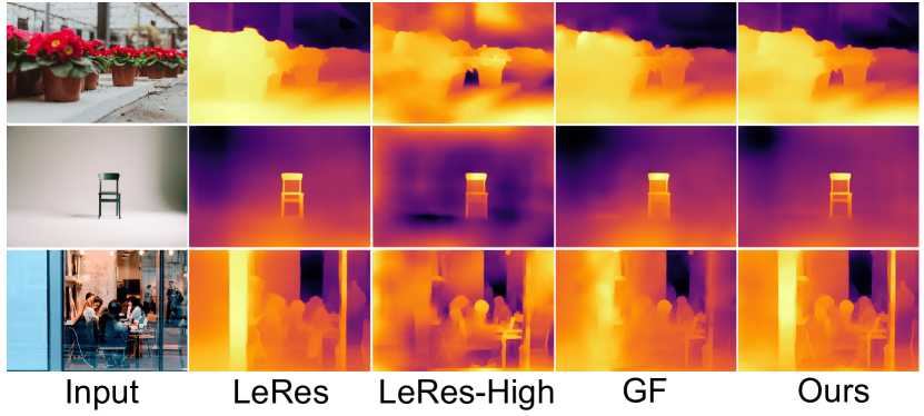
Figure 9: Three types of challenging cases, which are out-of-focus images, featureless regions, and transparent surfaces.

Our method benefits from details in high-resolution images. If the original resolution of input images are low, the improvements by our multi-resolution depth fusion are minor. Furthermore, there are other challenging cases for our method. As demonstrated in Fig. 9, the first scenario is out-of-focus images (the $1^{st}$ row). Since the out-of-focus regions are blurred, the details cannot be recovered by high resolution depth map. The second type is the featureless images. As shown in $2^{nd}$ row, the white floor and wall are featureless, and monocular depth estimation backbones cannot predict the accurate depth. The $3^{rd}$ case is transparent or reflective materials such as water and glasses. Since there is a glass wall in front of the scene, the depth enhancement results contain many artifacts.

5 Conclusion

We introduce a multi-resolution gradient-based depth map fusion pipeline to enhance the depth maps by backbone monocular depth estimation methods. Depth maps with a wide level of details are recovered by our method, which are helpful for many following and highly-related tasks such as image segmentation or 3D scene reconstruction. Comparing with prior works in depth map fusion, the proposed method has a great robustness to image noises, and runs in real time. The self-supervised training scheme also enables training on unlabeled images. Comprehensive evaluations and a large amount of ablations are conducted, proving the effectiveness of every critical modules in the proposed method.

Appendix A Supplementary material

A.1 Discussions on the multi-resolution theory

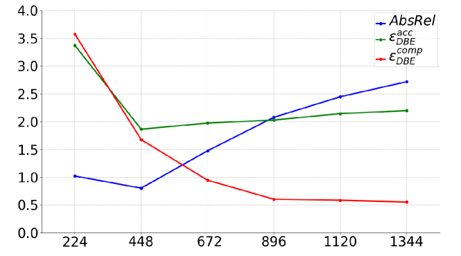
Figure 10: Evaluations of LeRes predictions on different input resolutions. X-axis denotes input resolutions, and y-axis denotes values of error metrics after scaling into the same range.

Our work is based on the observation that for fully convolutional monocular depth estimation networks, input images at training resolutions produce the highest accuracy in depth values, while high-resolution inputs lead to more details with inaccurate depth values. In order to test this multi-resolution theory, we adopt input images at 6 different resolutions to predict corresponding depth maps at different resolutions. We evaluate these predicted depth maps by several metrics. The evaluation is conducted on Ibims-1 (Koch et al. 2018) dataset, which provides images at the resolution of $640\times 480$. We utilize down-sampling and linear interpolation to change the resolutions from $224\times 224$ to $1344\times 1344$. We evaluate three metrics $AbsRel$, $\mathcal{E}^{acc}_{DBE}$ and $\varepsilon^{comp}_{DBE}$ provided by Ibims-1. While $AbsRel$ evaluate the global accuracy of the depth map, $\varepsilon^{acc}_{DBE}$ and $\mathcal{E}^{comp}_{DBE}$ evaluate the depth boundary accuracy error and the depth boundary completeness error, respectively. The three metrics are the lower the better. We test the depth prediction of LeRes at 6 different resolutions, the error values are plotted in Figure 10 with qualitative results demonstrated in Figure 11. The training resolution of LeRes is $448\times 448$, this resolution at Figure 10 achieves the lowest $AbsRel$ proving the correctness of our method to fuse depth values from training resolutions (low-resolution in our method). Inputs smaller than $448\times 448$ are incorrect in both accuracy and details (high in all three metrics), and inputs larger than $448\times 448$ lead to good details (low in $\varepsilon^{comp}_{DBE}$) with inaccurate depth values (high in $AbsRel$). Since some boundaries are missing in the ground truths depth map, the boundary accuracy $\varepsilon_{DBE}^{acc}$ (Koch et al. 2018) increases a little bit. It is a common observation of fully convolutional neural networks. As long as two depth maps at training resolution and higher resolution are given, our fusion network can successfully fuse them into an overall plausible one by keeping both value accuracy and details, without any finetuning on backbone networks. It is why our depth fusion pipeline has a great generalization ability while changing backbones, no additional finetuning is needed.

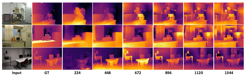
Figure 11: Visualizations of depth estimations at different input resolutions by LeRes (Yin et al. 2021).

A.2 Technical and implementation details

Implementation details

While incorporating on the backbone of LeRes (Yin et al. 2021), here we provide more details. Bilinear interpolation is adopted to generate the high-resolution input for our fusion framework from the original input. The training loss $l_{\text{mILNR}}$ and $l_{\text{rank}}$ is constructed with three levels of resolution, which are 512, 1024 and 2048.

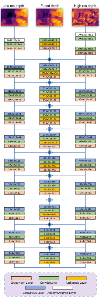
Figure 16: The network structure of our gradient-based composition module (the fusion network).

The detailed network structure of our fusion network is provided in Figure 16. Our network is end-to-end optimized using the AdamW (Loshchilov and Hutter 2017) optimizer with the batch size of 2, using HR-WSI (Xian et al. 2020) dataset as the training set. The initial learning rate is 0.0001, and 2 epochs of training on the whole 36 training sets are processed. For ablation study we trained on one training set for 30 epochs. The Cosine Annealing (Loshchilov and Hutter 2016) is adopted as the learning rate scheduler, and the decay rate is fixed as 0.99 every 100 steps. We implement our method on the Ubuntu22 system with one NVIDIA TITAN V GPU and a 16G RAM. The CUDA version is 11.1 and the Python version is 3.8. We use the depth prediction architecture proposed in LeRes (Yin et al. 2021) as monocular depth estimation backbone, consisting of two versions of encoders (ResNet50 (He et al. 2016) or ResNeXt101 (Xie et al. 2017)) and a decoder. We adopt ResNet50 as our encoder backbone through the whole evaluation process. To preprocess the HR-WSI dataset, the low-resolution inputs are resized to $448\times 448$, which is the default resolution of LeRes. High-resolution inputs are resized to $1344\times 1344$ to predict missing details. For radius and regularization parameters in guided filter, we fixed them as $\frac{W}{12}$ and $10^{-12}$ ($W$ denote the width of the input image). We find that radius larger than this value would cause blurry and regularization larger than this value would lose details. We use canny edge detection to select 7200 high quality guided filter results as our training set. The regular term $\sigma$ of ranking loss is fixed as 0.1, after testing values between $[0,1]$.

While LeRes and NeWCRFs predict inverse depth values, SGR, MiDas and DPT directly predict depth values. Thus, while using our fusion network trained with LeRes backbone, We transform the depth values predicted by SGR, MiDas and DPT to inverse depth by $D_{inverse}=D_{max}-D$ ($D_{max}$ is the maximum depth value in the whole depth map) before sending to the fusion network. The low resolution depth predictions of SGR, MiDas, DPT and NeWCRFs are set to $448\times 448$, $392\times 392$, $384\times 384$ and $640\times 480$ respectively, which are the same as their training resolution. For high resolution depth predictions, we set the resolution as $1344\times 1344$, $1176\times 1176$, $1152\times 1152$ and $1920\times 1440$ respectively. Changing the backbone from LeRes to others does not require any additional finetuning. All experimental results are got by testing for one time.

Details of training strategies

For robust training, we apply several training strategy to improve generalize ability of the model. Before fusion depth, we first scale the depth value by $D_{scaled}=MinMax(D_{pred})\times 2-1$ ($MinMax(D)=(D-D_{min})/(D_{max}-D_{min})$).We adopt data augmentation of random flipping of x,y axes and random transforming to inverse depth by $D_{input}=-D_{scaled}$ ($D_{scaled}$ is the depth value scaled to range $[-1,1]$.). Although the fusion network is trained to fuse both depth maps and inverse depth maps, while testing we feed inverse depth maps for all backbones for a fair comparison.

Besides, we adopt a multi-scale training strategy to supervise the intermediate results of the proposed fusion network. We adopt the same structure of our last decoding block but with different input channel number, to predict two additional fused depth maps at lower resolutions ($1024\times 1024$ and $512\times 512$). In our training process, the three fused depth maps at different resolutions are used to calculate the losses $l_{\text{mILNR}}$ and $l_{\text{rank}}$.

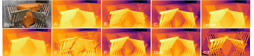
Figure 12: Visual comparison of different loss function settings. Our loss function design recovers the details correctly, while using ILNR loss (C and F) to learn the guided filter result leads to incorrect artifacts near the wall and desk.

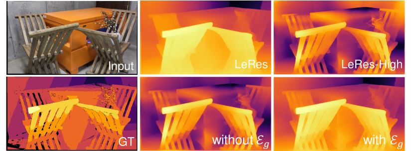
Figure 13: Visual comparisons of results with and without $\mathcal{E}_{g}$. Result without $\mathcal{E}_{g}$ contains many wrong depth relations from high resolution depth.

Sampling strategy of our ranking loss

Ranking loss is a widely used loss function for many metric learning tasks. It is constructed based on sampled pairs of pixels. However, previous ranking loss only focus on keeping the order while the value error is essential in our method for supervising the training of the gradient domain. We introduce a novel ranking loss which can constrain the value error as well as the order. Sample strategy of our method are presented below.

For monocular depth estimation task, DIW (Chen et al. 2016) adopt the pair-wise ranking loss to improve the prediction accuracy with a random sample strategy. SGR (Xian et al. 2020) propose the structure guided ranking loss by sampling points around instance boundaries. We follow the edge-guided sampling strategy of SGR (Xian et al. 2020), sample point-pairs near the depth boundaries. The depth boundaries are generated follow the pipeline of canny edge detection without denoise, and change the non-maximum suppression to threshold. We firstly utilize the Sobel operator to calculate the gradient maps of a depth map generated by guided filter we mentioned in our paper. After we get the gradient maps $G_{x}$, $G_{y}$ and gradient magnitude map $G$, we compute the depth boundaries map $E_{d}$ by thresholding the gradient magnitude map use the function as follow: $E_{d}=\mathbb{I}[G\geq(1-\alpha)\cdot\max(G)]$.

Here $\alpha$ is a threshold parameter to control the density of depth boundaries map. For each point $e=(x,y)$ in $E_{d}$, we sample four points $[e_{k}=(x_{k},y_{k}),k=a,b,c,d]$ alongside the gradient direction at point $e$ by equations as follow:

$$\left\{\begin{array}[]{lr}x_{k}=x+\delta_{k}G_{x}(e)/G(e)\\ y_{k}=y+\delta_{k}G_{y}(e)/G(e)\end{array}\right.$$ (10)

The parameters $\delta_{k}$ are generated randomly while make sure the sampled points are near the depth boundaries point $e$, and they are ordered as $\delta_{a}\textless\delta_{b}\textless 0\textless\delta_{c}\textless\delta_{d}$. To avoid sampled too far, we limit that $\left\|\delta_{k}\right\|\leq\beta$. We finally add $(e_{a},e_{b}),(e_{b},e_{c})and(e_{c},e_{d})$ into the point-pair set to calculate our novel ranking loss. We also apply the same sample strategy to $D_{high}$ and combine the point-pair set together. The calculation weights of point-pair set from $D_{gf}$ and $D_{high}$ are set as 12 and 8.

We use a indicator $Z_{ij}$ to define the relation of the point-pair $(e_{i},e_{j})$ which is

$$\left\{\begin{array}[]{ll}z_{ij}=1,&\frac{p_{gf}^{i}}{p_{gf}^{j}}\geq 1+\tau\;or\;\frac{p_{gf}^{i}}{p_{gf}^{j}}\leq\frac{1}{1+\tau}\\ z_{ij}=0,&otherwise\end{array}\right.$$ (11)

$\tau$ is the tolerance threshold of depth boundary which we set to 0.001. In our training process, we set $\alpha$ and $\beta$ as 0.15 and 60 respectively. For lower fused depth ($1024\times 1024$ and $512\times 512$) we set $\beta$ as 30 and 15. Other parameters are introduced in Section 3.3 of the main paper. Figure 14 gives out some visualization example of sampled points, which in input image are colored as green (left) while in depth map are colored as beige (right).

A.3 Detailed information of benchmarks

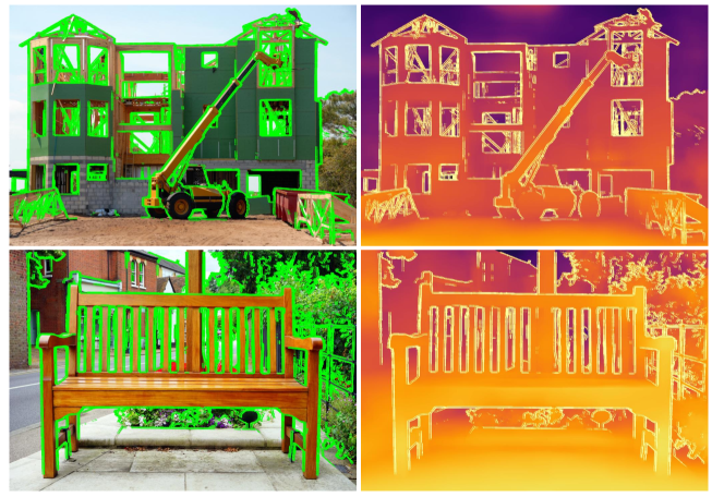
Figure 14: Visualizations of sample points. Here we set $\beta$ to 10 which makes the sample points being close to edges where gradients change most rapidly for better illustration.

Here we introduce several widely-used image datasets with depth ground truths.

Multiscopic (Yuan et al. 2021) dataset is an indoor dataset including real data collected by multi-lens cameras and synthetic data generated by renderers. The dataset contains 1100 scenes of synthetic data for training, 100 scenes of synthetic data for testing and 100 scenes of real data for other tasks. For each synthetic scene, Multiscopic (Yuan et al. 2021) provide 5 different views of RGB image and disparities, at a resolution of $1280\times 1080$. For each real scene, 3 different views of RGB images and disparities are provided.

Middlebury2021 (Scharstein et al. 2014) is a high quality stereo dataset collected by a structured light acquisition system. This dataset provides images and disparities for different indoor scenes at a resolution of $1920\times 1080$. The dataset contains 24 testing scenes with their calibration files respectively. At test time, we transform the disparity value $d$ to depth value $z$ by $z=baseline*f/(d+d_{offs})$, where the values of $baseline$, the focal length $f$ and the displacement of principal points $d_{offs}$ are provided in the dataset.

Hypersim (Roberts et al. 2021) is a photorealistic synthetic dataset for holistic indoor scene understanding. It contains 77400 images of 461 indoor scenes with per-pixel labels and corresponding ground truth geometry. Due to the large size of the whole dataset, we test on three subsets containing 286 tone-mapped images generated from their released codes.

NYUv2 (Nathan Silberman and Fergus 2012) dataset is a wildly-used indoor dataset that provides real data at the resolution of $640\times 480$. Data in the NYUv2 are captured by RGB and Depth cameras in the Microsoft Kinect. It includes 120K training images and 654 testing images. In evaluation, we use their official test split.

KITTI (Uhrig et al. 2017) is a outdoor stereo depth map dataset, providing thousands of raw LiDar scans and their corresponding RGB images. The stereo images and 3D laser scans of street scenes are captured by a moving vehicle. Images are at the resolution of $1216\times 352$. While the aspect ratio of these data is about 4:1, the depth maps collected by laser equipment exist a large amount of missing points. We test on its testing subset of 652 images.

For evaluation metrics mentioned in the main paper, the square relative error $SqRel$ is defined as $SqRel=\frac{1}{N}\sum(\frac{d_{i}^{*}-d_{i}}{d_{i}^{*}})^{2}$. The root mean square error $rms$ is defined as $rms=\sqrt{\frac{1}{N}\sum{\left\|d_{i}^{*}-d_{i}\right\|}^{2}}$.

A.4 Additional experiments and results

Evaluation on the backbone of Midas

In the paper, we provide the quantitative evaluation of our method on four monocular backbones, comparing with other fusion methods. Here We also provide the quantitative evaluation of our method on the backbone of MiDas to show the performance boost by our method. Quantitative results are in the Table  5. Besides the evaluation metrics mentioned in the paper, we also evaluate our method on MiDas using $ORD$ (Xian et al. 2020) and $D^{3}R$ (Miangoleh et al. 2021), which using the same evaluation function but with different sample strategy. The evaluation function of $D^{3}R$ is as follow: $D^{3}R=\frac{\sum_{k}w_{k}\mathbb{I}(Z_{ij}\neq Z^{*}_{ij})}{\sum_{k}w_{k}}$ , where $w_{k}$ is a weight set to 1 and $Z_{ij}$ denote the sampled pair-points relation of $e_{i}$ and $e_{j}$.

Methods	Multiscopic
	SqRel$\downarrow$	rms$\downarrow$	log10$\downarrow$	$\delta_{1}\uparrow$	$\delta_{2}\uparrow$	ORD$\downarrow$	$D^{3}R\downarrow$
MiDas	6.118	11.684	0.070	0.800	0.924	0.192	0.557
MiDas-GF	6.204	11.694	0.070	0.800	0.924	0.194	0.549
MiDas-Ours	6.034	11.602	0.070	0.801	0.925	0.190	0.536
Methods	Middlebury2021
	SqRel$\downarrow$	rms$\downarrow$	log10$\downarrow$	$\delta_{1}\uparrow$	$\delta_{2}\uparrow$	ORD$\downarrow$	$D^{3}R\downarrow$
MiDas	0.750	3.766	0.063	0.811	0.947	0.249	0.713
MiDas-GF	0.737	3.722	0.062	0.810	0.948	0.247	0.712
MiDas-Ours	0.72	3.67	0.062	0.816	0.949	0.244	0.703
Methods	Hypersim
	SqRel$\downarrow$	rms$\downarrow$	log10$\downarrow$	$\delta_{1}\uparrow$	$\delta_{2}\uparrow$	ORD$\downarrow$	$D^{3}R\downarrow$
MiDas	0.445	1.298	0.091	0.69	0.893	0.216	0.452
MiDas-GF	0.444	1.298	0.092	0.689	0.893	0.219	0.424
MiDas-Ours	0.428	1.275	0.09	0.694	0.895	0.212	0.396

Table 5: The quantitative evaluations on three benchmark datasets, comparing to a monocular depth estimation network MiDas (Ranftl et al. 2019), guided filter (“GF” in the table) and our method on the backbone of MiDas. Bold numbers denote the best performance of each metric. Our method achieve the best performance in these three benchmarks.

Visual comparisons

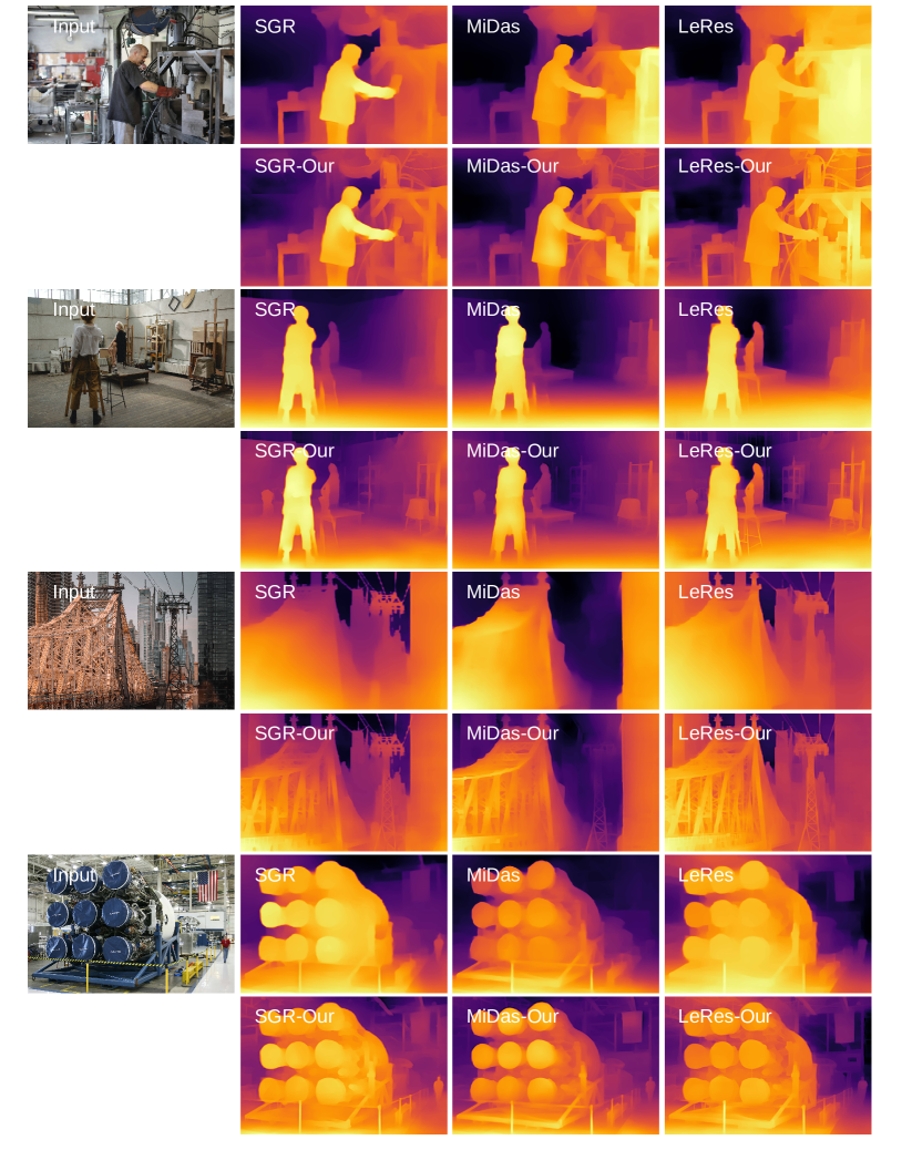
Figure 19: Visual results on Internet images.

Visualizations of depth enhancements on three backbones are in Figure 17 (for Middburry dataset) and Figure 18 (for Hypersim dataset). We also provide depth fusion results of our methods on three backbones on many Internet images in Figure 19-21. We can see from the figures that since images in Middburry dataset are at the resolution of $1920\times 1080$, the visual improvements by depth fusion are more obvious than low resolution images of $1024\times 768$ in Hypersim dataset. From the Internet images, the improvements are even better, since Internet images are at higher resolutions from $2590\times 1680$ to $8192\times 5462$. Therefore, our method produces more depth improvements on high resolution inputs, which is also the target scenario of the proposed method.

We also test our method on several Internet videos (see the videos shown on https://github.com/yuinsky/gradient-based-depth-map-fusion), by performing the proposed single-image pipeline frame by frame. Since each frame is processed separately, there are some inconsistencies among frames.

As introduced in ablation studies in the main paper, We also visualize results of different loss function settings (details about loss settings A to F are mentioned in Section 4.3 in the main paper) in Figure  12. We can see from the visualization results that using $l_{\text{mILNR}}$ to learn guided filter result leads to incorrect artifacts. We also visualize the depth fusion results with and without $\mathcal{E}_{g}$ in Figure 13, from which we found that the fused depth would not follow the depth values of low resolution depth while not using $\mathcal{E}_{g}$.

Noise robustness

As described in Section 4.2 of the main paper, we evaluate the anti-noise ability by testing on images with synthetic Gaussian or Pepper noises. Gaussian noises often exist when the field of view of the image sensor is not bright enough or the brightness is not uniform enough when shooting. The image sensor works for a long time and the temperature of the sensor is too high may also cause such noises. Salt and pepper noises, also known as impulse noises, are often caused by image clipping, randomly changes some pixel values to black or white. Such spot noise may also be generated by strong interference on the signal of image sensors and errors occurred in transmission or decoding process, etc.

Other than the error curves in Figure 8 of the main paper, here we provide two visual examples for better illustration. As in Figure 15, BMD (Miangoleh et al. 2021) suffers from image noises, while our method produce on-par results with and without noises.

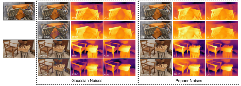
Figure 15: Illustrations of our results with different levels of Gaussian or Pepper noises, compared with a depth fusion alternative BMD (Miangoleh et al. 2021).

Methods	NYU
	SqRel$\downarrow$	rms$\downarrow$	log10$\downarrow$	$\delta_{1}\uparrow$	$\delta_{2}\uparrow$
LeRes	0.134	0.067	0.085	0.783	0.899
LeRes-GF	0.128	0.068	0.087	0.7756	0.896
LeRes-BMD	0.148	0.083	0.108	0.701	0.864
LeRes-Ours	0.122	0.073	0.094	0.748	0.885
Methods	KITTI
	SqRel$\downarrow$	rms$\downarrow$	log10$\downarrow$	$\delta_{1}\uparrow$	$\delta_{2}\uparrow$
LeRes	0.042	0.094	0.143	0.462	0.718
LeRes-GF	0.043	0.095	0.145	0.454	0.715
LeRes-BMD	0.045	0.098	0.149	0.450	0.704
LeRes-Ours	0.045	0.096	0.154	0.465	0.691

Table 6: Quantitative results on two low-resolution datasets NYU and KITTI.

Method	Task	Time per frame	GFLOPs
LeRes	pred low-res depth	0.0240s	95.88092G
	pred high-res depth	0.0958s	862.92825G
SGR	pred low-res depth	0.0282s	95.88092G
	pred high-res depth	0.0981s	862.92825G
3DK	pred refinement depth	0.0141s	118.02850G
BMD	pred refinement depth	14.614s	14834.4784G
Guided Filter	fuse low-res and high-res	0.7025s	-
Ours	fuse low-res and high-res	0.0653s	17.68863G

Table 7: Running time statistics. GFLOPs denotes G floating point operations, for evaluating the computational efficiency.

Evaluations on KITTI and NYUv2

Several depth fusion method including guided filter, BMD and ours are also tested on NYU and KITTI.

State-of-the-arts in monocular depth estimation such as LeRes and SGR, will downsample the high-resolution images to a lower training resolution, which for LeRes is $448\times 448$. Based on the observation that some information at original resolution would be lost in down-sampling, depth fusion method including guided filter, BMD and ours utilize such lost information to recover a detailed depth map from depth predictions at high resolutions. It means the original resolution of images should not be too low. If the original resolution in dataset is low, we cannot interpolate them to get more details.

The low-resolution input size of our model is $448\times 448$, and high-resolution input size is set as $1344\times 1344$. However, the original resolution of NYU is $640\times 480$, which is almost the same as our low-resolution resolution. The original resolution of KITTI is $1216\times 352$, which is also two low in height.

When tested on these datasets, the high-resolution input is obtained by interpolation operation, that means the high-resolution inputs do not contain much extra information compared with low-resolution inputs. The interpolation operations would even cause additional errors on predictions. Thus, depth fusion method are not effective on low-resolution datasets, and the test results also show our performance on NYU and KITTI is not better than monocular backbones.

Running time

Detailed running time and computational statistics of monocular depth backbones and depth fusion methods are in Table 7.

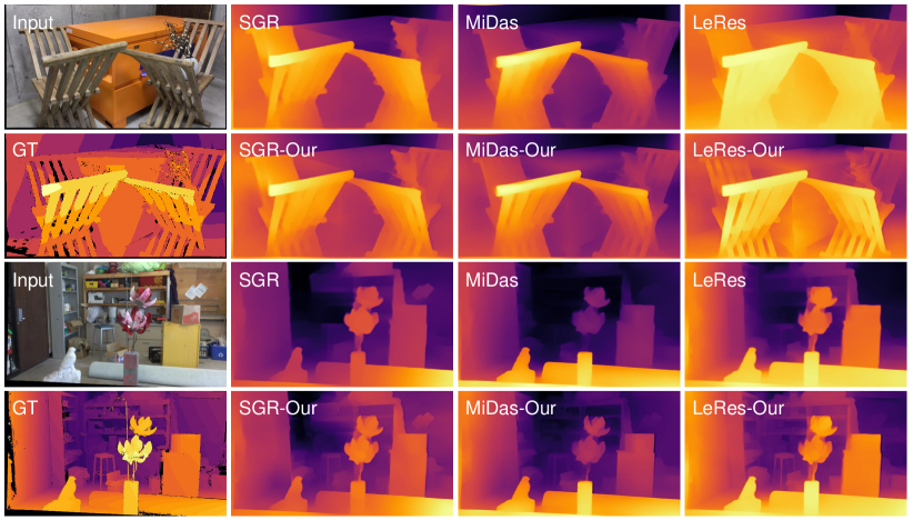
Figure 17: Visual results of data from Middlebury2021 dataset.

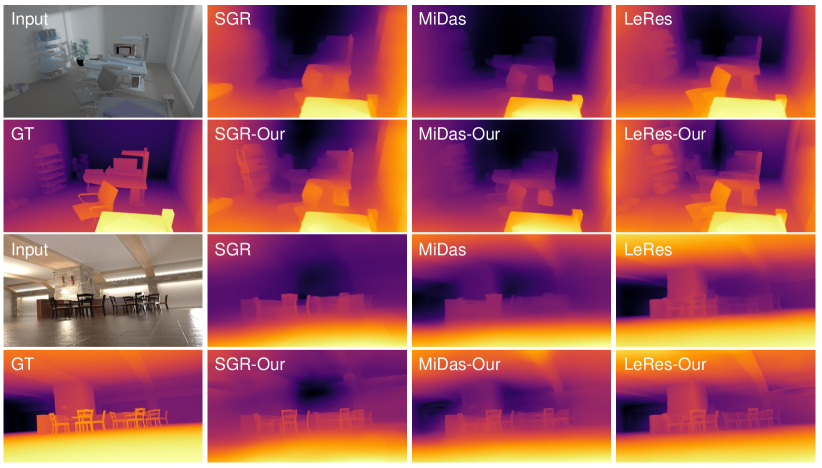
Figure 18: Visual results of data from Hypersim dataset.

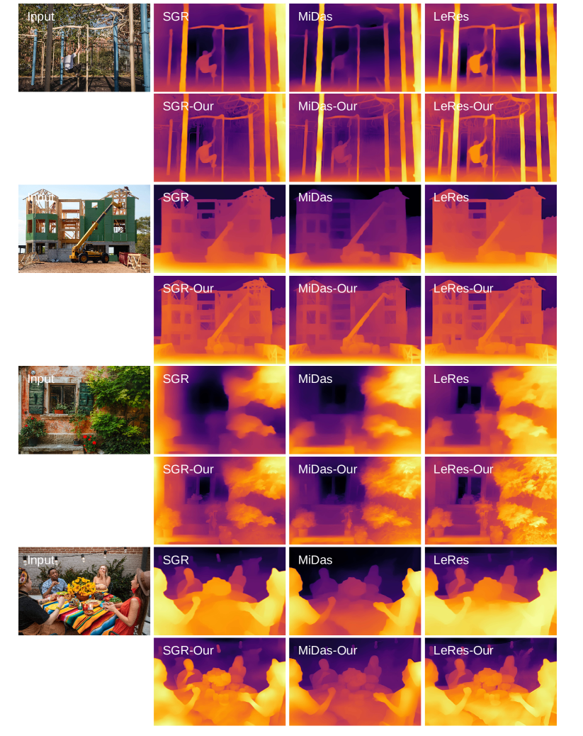
Figure 20: Visual results on Internet images.

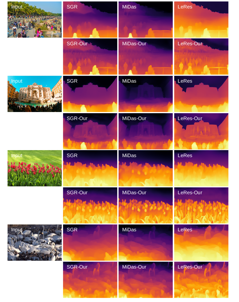
Figure 21: Visual results on Internet images.

References

- Amiri, Loo, and Zhang (2019) Amiri, A. J.; Loo, S. Y.; and Zhang, H. 2019. Semi-supervised monocular depth estimation with left-right consistency using deep neural network. In 2019 IEEE International Conference on Robotics and Biomimetics (ROBIO), 602–607. IEEE.
- Bailey and Durrant-Whyte (2006) Bailey, T.; and Durrant-Whyte, H. 2006. Simultaneous localization and mapping (SLAM): Part II. IEEE robotics & automation magazine, 13(3): 108–117.
- Bozorgtabar et al. (2019) Bozorgtabar, B.; Rad, M. S.; Mahapatra, D.; and Thiran, J.-P. 2019. Syndemo: Synergistic deep feature alignment for joint learning of depth and ego-motion. In Proceedings of the IEEE/CVF International Conference on Computer Vision, 4210–4219.
- Casser et al. (2019) Casser, V.; Pirk, S.; Mahjourian, R.; and Angelova, A. 2019. Depth prediction without the sensors: Leveraging structure for unsupervised learning from monocular videos. In Proceedings of the AAAI conference on artificial intelligence, volume 33, 8001–8008.
- Chen et al. (2016) Chen, W.; Fu, Z.; Yang, D.; and Deng, J. 2016. Single-image depth perception in the wild. Advances in neural information processing systems, 29: 730–738.
- Eigen, Puhrsch, and Fergus (2014) Eigen, D.; Puhrsch, C.; and Fergus, R. 2014. Depth map prediction from a single image using a multi-scale deep network. arXiv preprint arXiv:1406.2283.
- Feng and Gu (2019) Feng, T.; and Gu, D. 2019. Sganvo: Unsupervised deep visual odometry and depth estimation with stacked generative adversarial networks. IEEE Robotics and Automation Letters, 4(4): 4431–4437.
- Godard et al. (2019) Godard, C.; Mac Aodha, O.; Firman, M.; and Brostow, G. J. 2019. Digging into self-supervised monocular depth estimation. In Proceedings of the IEEE/CVF International Conference on Computer Vision, 3828–3838.
- Gwn Lore et al. (2018) Gwn Lore, K.; Reddy, K.; Giering, M.; and Bernal, E. A. 2018. Generative adversarial networks for depth map estimation from RGB video. In Proceedings of the IEEE Conference on Computer Vision and Pattern Recognition Workshops, 1177–1185.
- He, Sun, and Tang (2010) He, K.; Sun, J.; and Tang, X. 2010. Guided image filtering. In European conference on computer vision, 1–14. Springer.
- He et al. (2016) He, K.; Zhang, X.; Ren, S.; and Sun, J. 2016. Deep residual learning for image recognition. In Proceedings of the IEEE conference on computer vision and pattern recognition, 770–778.
- He et al. (2018) He, L.; Chen, C.; Zhang, T.; Zhu, H.; and Wan, S. 2018. Wearable depth camera: Monocular depth estimation via sparse optimization under weak supervision. IEEE Access, 6: 41337–41345.
- Heise et al. (2013) Heise, P.; Klose, S.; Jensen, B.; and Knoll, A. 2013. Pm-huber: Patchmatch with huber regularization for stereo matching. In Proceedings of the IEEE International Conference on Computer Vision, 2360–2367.
- Hubel and Wiesel (1962) Hubel, D. H.; and Wiesel, T. N. 1962. Receptive fields, binocular interaction and functional architecture in the cat’s visual cortex. The Journal of physiology, 160(1): 106–154.
- Jung et al. (2017) Jung, H.; Kim, Y.; Min, D.; Oh, C.; and Sohn, K. 2017. Depth prediction from a single image with conditional adversarial networks. In 2017 IEEE International Conference on Image Processing (ICIP), 1717–1721. IEEE.
- Koch et al. (2018) Koch, T.; Liebel, L.; Fraundorfer, F.; and Korner, M. 2018. Evaluation of cnn-based single-image depth estimation methods. In Proceedings of the European Conference on Computer Vision (ECCV) Workshops, 0–0.
- Kuznietsov, Stuckler, and Leibe (2017) Kuznietsov, Y.; Stuckler, J.; and Leibe, B. 2017. Semi-supervised deep learning for monocular depth map prediction. In Proceedings of the IEEE conference on computer vision and pattern recognition, 6647–6655.
- Levinson et al. (2011) Levinson, J.; Askeland, J.; Becker, J.; Dolson, J.; Held, D.; Kammel, S.; Kolter, J. Z.; Langer, D.; Pink, O.; Pratt, V.; et al. 2011. Towards fully autonomous driving: Systems and algorithms. In 2011 IEEE intelligent vehicles symposium (IV), 163–168. IEEE.
- Li et al. (2015) Li, B.; Shen, C.; Dai, Y.; Van Den Hengel, A.; and He, M. 2015. Depth and surface normal estimation from monocular images using regression on deep features and hierarchical crfs. In Proceedings of the IEEE conference on computer vision and pattern recognition, 1119–1127.
- Li and Snavely (2018) Li, Z.; and Snavely, N. 2018. Megadepth: Learning single-view depth prediction from internet photos. In Proceedings of the IEEE Conference on Computer Vision and Pattern Recognition, 2041–2050.
- Liu et al. (2015) Liu, F.; Shen, C.; Lin, G.; and Reid, I. 2015. Learning depth from single monocular images using deep convolutional neural fields. IEEE transactions on pattern analysis and machine intelligence, 38(10): 2024–2039.
- Loshchilov and Hutter (2016) Loshchilov, I.; and Hutter, F. 2016. Sgdr: Stochastic gradient descent with warm restarts. arXiv preprint arXiv:1608.03983.
- Loshchilov and Hutter (2017) Loshchilov, I.; and Hutter, F. 2017. Decoupled weight decay regularization. arXiv preprint arXiv:1711.05101.
- Mayer et al. (2016) Mayer, N.; Ilg, E.; Hausser, P.; Fischer, P.; Cremers, D.; Dosovitskiy, A.; and Brox, T. 2016. A large dataset to train convolutional networks for disparity, optical flow, and scene flow estimation. In Proceedings of the IEEE conference on computer vision and pattern recognition, 4040–4048.
- Miangoleh et al. (2021) Miangoleh, S. M. H.; Dille, S.; Mai, L.; Paris, S.; and Aksoy, Y. 2021. Boosting Monocular Depth Estimation Models to High-Resolution via Content-Adaptive Multi-Resolution Merging. In Proceedings of the IEEE/CVF Conference on Computer Vision and Pattern Recognition, 9685–9694.
- Nathan Silberman and Fergus (2012) Nathan Silberman, P. K., Derek Hoiem; and Fergus, R. 2012. Indoor Segmentation and Support Inference from RGBD Images. In ECCV.
- Niklaus et al. (2019) Niklaus, S.; Mai, L.; Yang, J.; and Liu, F. 2019. 3d ken burns effect from a single image. ACM Transactions on Graphics (TOG), 38(6): 1–15.
- Pérez, Gangnet, and Blake (2003) Pérez, P.; Gangnet, M.; and Blake, A. 2003. Poisson image editing. In ACM SIGGRAPH 2003 Papers, 313–318.
- Porter and Duff (1984) Porter, T.; and Duff, T. 1984. Compositing digital images. In Proceedings of the 11th annual conference on Computer graphics and interactive techniques, 253–259.
- Ranftl, Bochkovskiy, and Koltun (2021) Ranftl, R.; Bochkovskiy, A.; and Koltun, V. 2021. Vision transformers for dense prediction. In Proceedings of the IEEE/CVF International Conference on Computer Vision, 12179–12188.
- Ranftl et al. (2019) Ranftl, R.; Lasinger, K.; Hafner, D.; Schindler, K.; and Koltun, V. 2019. Towards robust monocular depth estimation: Mixing datasets for zero-shot cross-dataset transfer. arXiv preprint arXiv:1907.01341.
- Roberts et al. (2021) Roberts, M.; Ramapuram, J.; Ranjan, A.; Kumar, A.; Bautista, M. A.; Paczan, N.; Webb, R.; and Susskind, J. M. 2021. Hypersim: A Photorealistic Synthetic Dataset for Holistic Indoor Scene Understanding. In International Conference on Computer Vision (ICCV) 2021.
- Scharstein et al. (2014) Scharstein, D.; Hirschmüller, H.; Kitajima, Y.; Krathwohl, G.; Nešić, N.; Wang, X.; and Westling, P. 2014. High-resolution stereo datasets with subpixel-accurate ground truth. In German conference on pattern recognition, 31–42. Springer.
- Smolyanskiy, Kamenev, and Birchfield (2018) Smolyanskiy, N.; Kamenev, A.; and Birchfield, S. 2018. On the importance of stereo for accurate depth estimation: An efficient semi-supervised deep neural network approach. In Proceedings of the IEEE Conference on Computer Vision and Pattern Recognition Workshops, 1007–1015.
- Uhrig et al. (2017) Uhrig, J.; Schneider, N.; Schneider, L.; Franke, U.; Brox, T.; and Geiger, A. 2017. Sparsity Invariant CNNs. In International Conference on 3D Vision (3DV).
- Wang et al. (2015) Wang, P.; Shen, X.; Lin, Z.; Cohen, S.; Price, B.; and Yuille, A. L. 2015. Towards unified depth and semantic prediction from a single image. In Proceedings of the IEEE conference on computer vision and pattern recognition, 2800–2809.
- Wu et al. (2019) Wu, Z.; Wu, X.; Zhang, X.; Wang, S.; and Ju, L. 2019. Spatial correspondence with generative adversarial network: Learning depth from monocular videos. In Proceedings of the IEEE/CVF International Conference on Computer Vision, 7494–7504.
- Xian et al. (2018) Xian, K.; Shen, C.; Cao, Z.; Lu, H.; Xiao, Y.; Li, R.; and Luo, Z. 2018. Monocular relative depth perception with web stereo data supervision. In Proceedings of the IEEE Conference on Computer Vision and Pattern Recognition, 311–320.
- Xian et al. (2020) Xian, K.; Zhang, J.; Wang, O.; Mai, L.; Lin, Z.; and Cao, Z. 2020. Structure-guided ranking loss for single image depth prediction. In Proceedings of the IEEE/CVF Conference on Computer Vision and Pattern Recognition, 611–620.
- Xie et al. (2017) Xie, S.; Girshick, R.; Dollár, P.; Tu, Z.; and He, K. 2017. Aggregated residual transformations for deep neural networks. In Proceedings of the IEEE conference on computer vision and pattern recognition, 1492–1500.
- Yin et al. (2021) Yin, W.; Zhang, J.; Wang, O.; Niklaus, S.; Mai, L.; Chen, S.; and Shen, C. 2021. Learning to recover 3d scene shape from a single image. In Proceedings of the IEEE/CVF Conference on Computer Vision and Pattern Recognition, 204–213.
- Yuan et al. (2022) Yuan, W.; Gu, X.; Dai, Z.; Zhu, S.; and Tan, P. 2022. NeWCRFs: Neural Window Fully-connected CRFs for Monocular Depth Estimation. In Proceedings of the IEEE Conference on Computer Vision and Pattern Recognition.
- Yuan et al. (2021) Yuan, W.; Zhang, Y.; Wu, B.; Zhu, S.; Tan, P.; Wang, M. Y.; and Chen, Q. 2021. Stereo Matching by Self-supervision of Multiscopic Vision. In 2021 IEEE/RSJ International Conference on Intelligent Robots and Systems (IROS), 5702–5709. IEEE.
- Zhang et al. (2018) Zhang, Z.; Cui, Z.; Xu, C.; Jie, Z.; Li, X.; and Yang, J. 2018. Joint task-recursive learning for semantic segmentation and depth estimation. In Proceedings of the European Conference on Computer Vision (ECCV), 235–251.
- Zhu et al. (2018) Zhu, C.; Xu, K.; Chaudhuri, S.; Yi, R.; and Zhang, H. 2018. SCORES: Shape composition with recursive substructure priors. ACM Transactions on Graphics (TOG), 37(6): 1–14.
- Zwald and Lambert-Lacroix (2012) Zwald, L.; and Lambert-Lacroix, S. 2012. The berhu penalty and the grouped effect. arXiv preprint arXiv:1207.6868.