Polaron with Quadratic Electron-phonon Interaction

Abstract

We present the first numerically exact study of a polaron with quadratic coupling to the oscillator displacement, using two alternative methodological developments. Our results cover both anti-adiabatic and adiabatic regimes and the entire range of electron-phonon coupling $g_{2}$, from the system’s stability threshold at attractive $g_{2}=-1$ to arbitrary strong repulsion at $g_{2}\gg 1$. Key properties of quadratic polarons prove dramatically different from their linear counterparts. They (i) are insensitive even to large quadratic coupling except in the anti-adiabatic limit near the threshold of instability at attraction; (ii) depend only on the adiabatic ratio but are insensitive to the electron dispersion and dimension of space; (iii) feature weak lattice deformations even at the instability point. Our results are of direct relevance to properties of electrons at low densities in polar materials, including recent proposals for their superconducting states.

The first results on polarons with quadratic coupling to phonons were reported in Refs. [1, 2], which explored properties of large-radius solitons in the adiabatic limit at strong coupling. Indications that nonlinear coupling to atomic displacements is important were found in several materials such as doped manganites [3], halide perovskites [4], and quantum paraelectrics [5]. Most notable is the unusual $T^{2}$ dependence of resistivity at high temperature, which was explained by considering electron-phonon interactions (EPI) with quadratic dependence on the phonon coordinates [5, 6]. The soft vibrational modes in these materials are transverse optical (TO) phonons for which the linear EPI is suppressed in the long-wave limit. However, local electron density changes the potential acting on nearby atoms and this change may increase or decrease the local spring constants. Early suggestions that bi-phonon exchange could be an important pairing mechanism at low doping [7] were recently revisited by quantifying and employing them for explaining the superconducting properties of SrTiO₃ [8, 9, 10]. While the treatment of the problem was perturbative, the dimensionless coupling constant was estimated to be of order unity, raising the question of consistency.

In the low-density limit—when the polaron physics is most relevant [11]—the key assumption on which the Migdal-Eliashberg theory is based (irrelevance of vertex corrections at strong coupling), namely $E_{F}\gg\Omega$, where $E_{F}$ is the Fermi energy and $\Omega$ is the characteristic phonon frequency, fails. Thus, any quantitative study of strong EPI effects in this limit should start from precise calculations of basic polaron properties such as its energy, $E$, effective mass, $m_{*}$, and the quasiparticle residue, $Z$. We are aware of only few theoretical attempts to account for quadratic EPI beyond perturbation theory. The original work [1, 2] was based on a variational approach for large-radius soliton-type solutions. A nonperturbative momentum average approximation [12] was used to study the interplay between linear (Holstein model [13]) and non-linear EPI at zero temperature in Refs. [14, 15]. Effects of non-linear EPI on the formation of charge density waves, superconductivity, and quasi-particle properties were investigated in a series of papers [16, 17, 18]. These determinant Monte Carlo [19] studies considered finite clusters (up to $N=8\times 8$ sites) in two dimensions at high electron density and finite temperature. More recently, the interplay between linear and quadratic EPI in the Fröhlich model of continuous space polarons was studied at zero temperature in Ref. [20] using variational Feynman’s path integral method [21].

All studies find that quadratic interaction with positive/negative coupling constant decreases/increases the effective strength of the linear EPI. However, none of the previous work was able to treat effects of strong quadratic coupling in the thermodynamic limit without approximations, or was investigating polaron properties for purely quadratic interaction. Meanwhile, as was mentioned above, there exist important cases when coupling to soft transverse phonons has no linear terms in the long-wave limit, e.g. quantum paraelectrics [5] and optically pumped systems [22, 23].

In this Letter, we employ two complementary numerically exact methods to solve the polaron model with quadratic coupling to atomic displacements, or $X^{2}$-polarons, at zero temperature. The first one is based on Feynman diagrams and is best suited for studying dispersive phonons in the regimes of weak and intermediate coupling. The second method—performing best at strong coupling and becoming particularly simple in the dispersionless regime —works with the path-integral representation for both the electron and atomic displacements. The two methods are new methodological advances that go well beyond previous developments. We explore both adiabatic and non-adiabatic limits and find that $X^{2}$-polarons remain well-defined all the way to the instability threshold and possess the remarkable ability (especially in the adiabatic case) to resist renormalization even in the extreme strong coupling limit.

Model. The key difference between our Hamiltonian and the well-studied Holstein model [13] is the quadratic, instead of linear, coupling to the local oscillator coordinates, $X_{i}=[b_{i}^{\dagger}+b_{i}^{\,}]/\sqrt{2M\Omega}\equiv x_{i}/\sqrt{2M\Omega}$, where $M$ and $\Omega$ are the oscillator mass and frequency, respectively (we use standard notation for on-site creation/annihilation operators for harmonic modes and electrons):

$$H=-t\sum_{<ij>}a_{j}^{\dagger}a_{i}^{\,}+\Omega\sum_{i}b_{i}^{\dagger}b_{i}^{\,}+\frac{\Omega}{4}g_{2}\sum_{i}n_{i}[b_{i}^{\dagger}+b_{i}^{\,}]^{2}\,.$$ (1)

Here $n_{i}=a_{i}^{\dagger}a_{i}^{\,}$ is the electron occupation number. The first two terms describe the electron hopping between nearest neighbor sites on the simple cubic lattice (in what follows we take $t$ as the unit of energy) and the local vibration modes, respectively. We count oscillator energies from their ground states, and use the dimensionless constant $g_{2}$ to parameterize the coupling. By writing the local potential energy for $n_{i}=1$ as $M\Omega^{2}[1+g_{2}]X_{i}^{2}/2$, we observe that (i) the model becomes unstable at $g_{2}\leq-1$, implying that the radius of convergence for a perturbative treatment in powers of $g_{2}$ is unity, (ii) the oscillator frequency is renormalized to

$$\tilde{\Omega}=r\Omega,\qquad r=\sqrt{1+g_{2}}\,,$$ (2)

and (iii) its ground state energy shifts to $\Omega(r-1)/2$.

Momentum-space representation (see also Supplemental material [24]). The first scheme is based on the Diagrammatic Monte Carlo (DiagMC) technique introduced in Ref. [25] and further developed in Ref. [26]. The imaginary-time Green’s function, $G(\mathbf{k},\tau)$, for momentum state $\mathbf{k}$ is sampled stochastically from the series expansion in powers of $g_{2}$ expressed as Feynman diagrams in terms of bare electron and phonon propagators. The difference between linear and quadratic coupling is a more complex set of diagram topologies consisting of a set of $n$-phonon loops because now each interaction vertex involves two phonons (instead of one) being emitted or absorbed (see Eq. (1)).

Figure 1 shows typical low-order diagrams. The simplest self-energy diagram is given by the 1-loop; its series, see Fig. 2, is absorbed into the “bare” electronic propagator, $G_{0}\to\tilde{G}_{0}$, by shifting the tight-binding dispersion $\epsilon_{\mathbf{k}}\to\tilde{\epsilon}_{\mathbf{k}}=\epsilon_{\mathbf{k}}+g_{2}\Omega/4$:

$$\tilde{G}_{0}(\mathbf{k},\tau)=e^{-\tilde{\epsilon}_{\mathbf{k}}\tau},\qquad D_{0}(\mathbf{q},\tau)=e^{-\Omega\tau}\,.$$ (3)

The remaining high-order loops display a wide variety of topologies that increase dramatically with the order of the diagram. In addition, there exist multiple Wick pairings that are topologically equivalent and result in the same contribution, meaning that each diagram comes with the combinatorial factor $2^{N_{\text{V}}-N_{2}}$, where $N_{\text{V}}$ is the total number of vertices and $N_{2}$ is the number of 2-phonon loops, i.e. loops consisting of two phonon propagators. The sign of the diagram is given by $(-g_{2})^{N_{\text{V}}}$, meaning that the expansion is sign-positive for $g_{2}<0$.

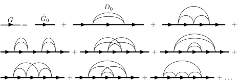
Figure 1: Momentum-space diagrams for the Green’s function up to fourth order in the quadratic coupling.

Figure 2: The geometric series of the 1-loop diagrams defines the “Hartree” renormalized electron propagator.

An ergodic sampling scheme includes the following updates:
Add/remove 2-loop: Seed time, $\tau_{1}$ and $\tau_{2}$, and momentum, $\mathbf{q}_{1}$ and $\mathbf{q}_{2}$, variables for new vertices to be added to the diagram and balance this proposal by suggesting to remove any of the existing 2-loops.
Add/remove 3-loop: This update is a straightforward generalization of the previous one, but for 3-loops. It is required for the generation of odd-order diagrams.
Relink: Pick any two phonon propagators across the whole diagram at random such that they do not share vertices, i.e. they start and end on four different vertices. Propose a new diagram topology by connecting the four vertices with the two phonon propagators randomly.
Additional updates, such as changing time and/or momentum variables of the diagram, are introduced to improve the autocorrelation time.

Following Ref. [26], the simulation is extended to the $N$-phonon Green’s function, which allows one to collect information about the structure of the phonon cloud. We employ standard procedures to extract the ground state energy, $E$, quasiparticle weight, $Z$, average number of phonons, $\langle N_{\rm ph}\rangle$, and effective mass, $m_{*}$, of the polaron.

Figure 3: Polaron properties (energy, effective mass, and $Z$-factor) in the adiabatic regime $\Omega/W=1/48$ (bandwidth $W=12t$ in 3D) as functions of EPI coupling.

X-representation approach. As discussed in Ref. [27], see also the Supplemental Material [24], any non-linear coupling to local vibration modes can be dealt with exactly and efficiently by specifying dimensionless atomic coordinates $x_{i}$ for all sites connected by the electron hopping transitions. The only new ingredient required for adapting the scheme of Ref. [27] to the model in Eq. (1) is the imaginary-time oscillator propagator in the presence of the electron

$$\tilde{U}(y,x,\tau)=e^{(1/2)\Omega\tau-\tilde{Q}(y,x,\tau)}\sqrt{\frac{r}{4\pi\sinh(\tilde{\Omega}\tau)}}\,\,,$$

$$\tilde{Q}(y,x,\tau)\,=\,\frac{r[\cosh(\tilde{\Omega}\tau)(x^{2}+y^{2})-2xy]}{4\sinh(\tilde{\Omega}\tau)}\,.$$ (4)

For empty sites, the “bare” propagator $U(y,x,\tau)$ has the same functional form as $\tilde{U}(y,x,\tau)$ but with $r=1$ and $\tilde{\Omega}=\Omega$. Thus, for any electron’s lattice path and any set of atomic displacements on sites connected by hopping transitions, one has an exact sign-positive expression for the system’s evolution operator subject to stochastic sampling without a bias.

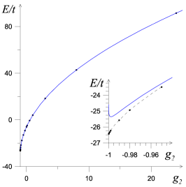
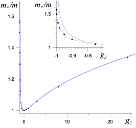
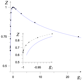
Figure 4: Polaron properties (energy, effective mass, and $Z$-factor) in the anti-adiabatic regime $\Omega/W=4$ in 3D as functions of EPI coupling. Solid lines are the analytic predictions based on the atomic limit (6)–(10); dashed lines connecting data points are used to guide an eye.

In the so-called atomic limit (AL), $t=0$, the solution for the Green’s function immediately follows from the Gaussian integral $G_{A}(\tau)=\int dxdyU(x)\tilde{U}(x,y,\tau)U(y)$ leading to

$$G_{A}(\tau)=Z_{A}e^{-E_{A}\tau}\left[1-\left(\frac{1-r}{1+r}\right)^{2}e^{-2\tilde{\Omega}\tau}\right]^{-1/2}\,,$$ (5)

where

$$Z_{A}=\frac{2\sqrt{r}}{1+r}\,,\qquad E_{A}=\frac{\Omega}{2}(r-1)\,.$$ (6)

The spectral density, defined by $G_{A}(\tau)=\int_{0}^{\infty}d\omega A_{A}(\omega)e^{-\omega\tau}$, is readily obtained by Taylor expanding $G_{A}(\tau)$ in powers of $e^{-2\tilde{\Omega}\tau}$:

$$A_{A}(\omega)=\sum_{k=0}^{\infty}Z_{2k}\delta(\omega-E_{2k})\;.$$ (7)

It is a set of $\delta$-functions at frequencies $E_{2k}=E_{A}+2k\tilde{\Omega}$ with $Z_{2k}$-factors equal to

$$Z_{2k}=Z_{A}\frac{(2k-1)!!}{2k!!}\left[\frac{1-r}{1+r}\right]^{2k}\;.$$ (8)

Finally, the atomic limit admits an exact solution for the average number of phonons in the polaron cloud defined as in Ref. [26]

$$\langle N_{\rm ph}\rangle=\sum_{k=0}^{\infty}(2k)Z_{2k}=\frac{(1-r)^{2}}{4r}\;.$$ (9)

If both $\tilde{\Omega}$ and $\Omega$ are much larger than $t$ (meaning that to the leading approximation the oscillators always remain in the ground state as the electron moves), then the finite-$t$ effects can be fully characterized by the overlap integral squared between the bare and renormalized ground states equal to $Z_{A}$:

$$E=-6Z_{A}t+E_{A}\,,\qquad m_{*}/m=Z_{A}^{-1}\;.$$ (10)

Results. In sharp contrast to conventional polarons, properties of $X^{2}$-polarons strongly depend on the sign of $g_{2}$, see Figs. 3 and 4. The effective mass (quasiparticle weight) goes through a minimum (maximum) at $g_{2}=0$, while the energy is an increasing function of $g_{2}$. The asymmetry is especially notable in the anti-adiabatic case $\Omega/W=4$, see Fig. 4, and is directly linked to the fact that at $g_{2}\to-1$ the local phonon frequency undergoes a dramatic change and ultimately softens to zero. Correspondingly, as long as the condition $\tilde{\Omega}>W$ is satisfied, the atomic-limit expressions featuring square-root singularities, see Eqs. (5)–(10), provide an accurate description of the polaron properties. However, on approach to the stability threshold, this condition ultimately gets violated and the singularity is removed because an electron moves away before the slow phonon mode has a chance to adjust to its interacting ground state. This explains the remarkable fact, that all polaron properties remain well defined and regular in the $g_{2}\to-1$ limit for any finite value of $t$, see Figs. 4 and 5.

For positive $g_{2}$, all properties change gradually even at $g_{2}\gg 1$. Moreover, in the adiabatic limit $\Omega/W=1/48$, see Fig. 3, both $Z$ and $m_{*}/m$ remain close to unity with sub percent accuracy for any $|g_{2}|\leq 1$. One way to interpret the data is to make a connection with the linear problem where the crossover from weak to strong coupling takes place when the dimensionless coupling $\lambda$, defined as the ratio between the coupling strength squared and the product of $W/2$ and $\Omega$, is of the order of unity. Introducing a similar parameter for model (1) we get $\lambda=2(g_{2}\Omega/4)^{2}/(W\Omega)=(g_{2}^{2}\Omega)/(8W)$. Its value for $|g_{2}|=1$ is $\lambda=1/384$ for the adiabatic case shown in Fig. 3 and $\lambda=1/2$ for the anti-adiabatic case shown in Fig. 4.

Another stark difference between linear and quadratic couplings is found in the structure of the lattice distortion dragged along by polarons. It is quantified through probabilities $Z_{n}$ of having $n$ virtual phonons in the ground state [for AL it is given by Eq. (8)]. In the linear case, the peak in $Z_{n}$ shifts from $n=0$ at weak coupling to large finite values of $n$ at strong coupling [26, 28]. In contrast, $Z_{n}$ for $X^{2}$-polarons is peaked at $n=0$ and decreases exponentially at large $n$ (Fig. 5b) for any value of negative $g_{2}$, including the close vicinity of the instability point $(1+g_{2})<10^{-3}$ when the average phonon number of phonons $\langle N_{\rm ph}\rangle$ is already large (Fig. 5a). Somewhat counter-intuitively, $Z_{n=0}$ for the moving particle ($t>0$) is larger than for the localized particle in the AL ($t=0$), whereas for large $n$ the opposite is true, see inset in Fig. 5a. Only for large $g_{2}$ in the deep adiabatic limit $\Omega/t\ll 1$ it is possible that $Z_{n}$ has a peak at finite $n$ due to formation of the soliton state [1].

We also find that properties of quadratic polarons mostly depend on the particle bandwidth, and are rather insensitive to the form of the dispersion relation and even the dimension of space, e.g., $E$, $Z$, $\langle N_{\rm ph}\rangle$, and $m_{*}$ are practically indistinguishable between the 3D and 1D cases provided the bandwidth is the same (see Supplemental material [24]).

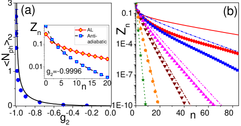
Figure 5: Phonon cloud in the anti-adiabatic limit in 3D at $\Omega/W=4$. (a) Average number of phonons $\langle N_{\rm\scriptsize ph}\rangle$ (blue circles) and the AL prediction (line), Eq. (9), for negative coupling constant. (b) Phonon distributions $Z_{n}$ in the polaron cloud (symbols) and the AL prediction (lines, Eq. (8)), $g_{2}=$: $-0.25$ (stars, dotted line), $-0.75$ (circles, dashed line), $-0.95$ (triangles down, dash-dot line), $-0.98$ (triangles up, dash-dot-dot line), $-0.998$ (squares, short-dash-dot line), and $-0.9996$ (diamonds, solid line). Inset in panel (a) shows the phonon distribution (squares) and Eq. (8) (diamonds) for $g_{2}=-0.9996$ on a smaller scale.

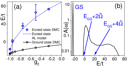
Figure 6: Anti-adiabatic limit in 3D at $\Omega/W=4$. (a) Ground state energy (circles connected by the black line) and that of the first excited state (blue diamonds). Blue dashed line is the first excited state energy in the AL. Vertical line at $g_{2}=-0.95$ corresponds to the coupling for which the spectral function $A(\omega)$ in panel (b) is shown. (b) Spectral function $A(\omega)$ at $g_{2}=-0.95$ for which Eq. (2) predicts $\widetilde{\Omega}\approx 10.7$. Arrows show energies of 2-phonon $2\tilde{\Omega}$ and 4-phonon $4\tilde{\Omega}$ thresholds above the ground state energy.

To complete the picture, we performed analytic continuation of the Green’s function spectral density, $A(\omega)$, in the anti-adiabatic limit by the Stochastic Optimization with Consistent Constraints method [26, 29]. In Figure 5b, we show the extracted positions of excited states and how they compare with the AL predictions (Fig. 5a). One can see in Fig. 5b that the onsets of high energy peaks are well described by energies $E_{2k}$ in Eq. (7).

Conclusions. We find that properties of $X^{2}$-polarons are dramatically different from those based on the intuition gained during a long history of Holstein polaron studies. In the adiabatic regime, $X^{2}$-polarons are nearly indistinguishable from bare particles for any coupling with $|g_{2}|\sim 1$. In the anti-adiabatic regime, particle properties are renormalized more strongly (but saturate to finite values) when approaching the instability threshold at $g_{2}=-1$, but remain small for positive $g_{2}$ except in the limit of large coupling. Perhaps the most unexpected result is that the lattice deformation around the $X^{2}$-polaron remains weak even at the threshold. This outcome explains the success of recent work on superconductivity in SrTiO₃ [8, 9, 10] which treated electrons as bare particles.

We established that the adiabatic ratio $\Omega/W$ is the key parameter to pay attention to for this problem, while other microscopic details and even the system dimension are less relevant. This fact can be used for the development of approximate schemes, such as momentum average [12], dynamical mean field theory [30], or many body approach [31] in the low density limit, that can then be validated against our numerically exact results.

The soliton-type solutions [1] cannot form for model parameters simulated in this work. The minimal requirement is to have $m_{*}/m\gg 1$ at $\Omega\ll\tilde{\Omega}\leq t$, which is not satisfied even for the ($\Omega/t=0.1$, $\tilde{\Omega}=30\Omega$) parameter set, for which we find $m_{*}/m\approx 3$. Future work should address the soliton problem under the assumption that the crystal is in close proximity to the quantum critical point when $\Omega\to 0$ and the electron contribution to the local vibrational energy is finite when $\tilde{\Omega}\to$ const.

NP, BS, AK, and ZZ acknowledge support from the National Science Foundation under grants DMR-2032136 and DMR-2032077. NN and ASM are supported by JST CREST Grant No. JPMJCR1874, Japan. MH, SK, and JT acknowledge funding by the Research Foundation - Flanders, projects GOH1122N, G061820N, G060820N, and by the University Research Fund (BOF) of the University of Antwerp. CF, SR, TH, and SK acknowledge support from the Austrian Science Fund (FWF) projects I 4506 (FWO-FWF joint project). The computational results presented have been achieved in part using the Vienna Scientific Cluster (VSC).

References

- [1] A. B. Kuklov, Phys. Lett. A 139, 270 (1989).
- [2] A. O. Gogolin and A. S. Ioselevich, Pis’ma Zh. Eksp. Teor. Fiz. 53(9), 456 (1991) [JETP Lett. 53, 479 (1991)].
- [3] V. Esposito, M. Fechner, R. Mankowsky, Phys. Rev. Lett. 118, 247601 (2017).
- [4] M. J. Schilcher, P. J. Robinson, D. J. Abramovitch et. al., ACS Energy Lett. 6, 2162 (2021).
- [5] A. Kumar, V. I. Yudson, and D. L. Maslov, Phys. Rev. Lett. 126, 076601 (2021).
- [6] K. G. Nazaryan and M. V. Feigel’man, Phys. Rev. B 104, 115201 (2021).
- [7] K. L. Ngai, Phys. Rev. Lett. 32, 215 (1974).
- [8] D. van der Marel, F. Barantani, and C. W. Rischau, Phys. Rev. Research 1, 013003 (2019).
- [9] P. A. Volkov, P. Chandra, and P. Coleman, Nature Comm. 13, 4599 (2022).
- [10] D. Kiseliov and M. Feigel’man, Phys. Rev. B 104, L220506 (2021).
- [11] A. S. Mishchenko, I. S. Tupitsyn, N. Nagaosa, and N. Prokof’ev, Scientific Reports 11, 9699 (2021).
- [12] M. Berciu, Phys. Rev. Lett. 97, 036402 (2006).
- [13] T. Holstein, Ann. Phys. 8, 325 (1959).
- [14] C. P. J. Adolphs and M. Berciu, EPL 102, 47003 (2013).
- [15] C. P. J. Adolphs and M. Berciu, Phys. Rev. B 89, 035122 (2014).
- [16] S. Li and S. Johnston, EPL 109, 27007 (2015).
- [17] S. Li, E. A. Nowadnick, and S. Johnston, Phys. Rev. B 92, 064301 (2015).
- [18] P. M. Dee, J. Coulter, K. G. Kleiner and S. Johnston, Commun. Phys. 3:145 (2020).
- [19] S. Johnston, E. A. Nowadnick, Y. F. Kung, B. Moritz, R. T. Scalettar, and T. P. Devereaux, Phys. Rev. B 87, 235133 (2013).
- [20] M. Houtput and J. Tempere, Phys. Rev. B 103, 184306 (2021).
- [21] R. P. Feynman, Phys. Rev. 97, 660 (1955).
- [22] D. M. Kennes, E. Y. Wilner, D. R. Reichman, and A. J. Millis, Nat. Phys. 13, 479 (2017).
- [23] J. Sous, B. Kloss, D. M. Kennes, D. R. Reichman, and A. J. Millis, Nat. Commun. 12, 5803 (2021).
- [24] See Supplemental Material.
- [25] N. V. Prokof’ev and B. V. Svistunov, Phys. Rev. Lett. 81, 2514 (1998).
- [26] A. S. Mishchenko, N. V. Prokof’ev, A. Sakamoto, and B. V. Svistunov, Phys. Rev. B 62, 6317 (2000).
- [27] N. Prokof’ev and B. Svistunov, Phys. Rev. B 106, L041117 (2022).
- [28] T. Hahn, N. Nagaosa, C. Franchini, and A. S. Mishchenko, Phys. Rev. B 104, L161111 (2021).
- [29] O. Goulko, A. S. Mishchenko, L. Pollet, N. Prokof’ev, and B. Svistunov, Phys. Rev. B 95, 014102 (2017).
- [30] P. Mitrić, V. Janković, N. Vukmirović, and D. Tanasković, Phys. Rev. Lett. 129, 096401 (2022).
- [31] A. S. Mishchenko, N. Nagaosa, and N. Prokof’ev, Phys. Rev. Lett. 113, 166402 (2014).