Signal enhancement for two-dimensional cryo-EM data processing

Abstract

Different tasks in the computational pipeline of single-particle cryo-electron microscopy (cryo-EM) require enhancing the quality of the highly noisy raw images. To this end, we develop an efficient algorithm for signal enhancement of cryo-EM images. The enhanced images can be used for a variety of downstream tasks, such as 2-D classification, removing uninformative images, constructing ab initio models, generating templates for particle picking, providing a quick assessment of the data set, dimensionality reduction, and symmetry detection. The algorithm includes built-in quality measures to assess its performance and alleviate the risk of model bias. We demonstrate the effectiveness of the proposed algorithm on several experimental data sets. In particular, we show that the quality of the resulting images is high enough to produce ab initio models of $\sim 10$ Å resolution. The algorithm is accompanied by a publicly available, documented and easy-to-use code.

1 Introduction

In the past few years, single-particle cryo-electron microscopy (cryo-EM) has become the state-of-the-art method for resolving the atomic structure and dynamics of biological molecules [12, 17, 2, 21, 22]. A cryo-EM experiment results in a large set of images, each corresponding to a noisy tomographic projection of the molecule of interest, taken from an unknown viewing direction. In addition, the electron doses transmitted by the microscope must be kept low to prevent damage to the radiation-sensitive biological molecules, inducing signal-to-noise ratio (SNR) levels that might be as low as -20dB (i.e., the power of the noise is 100 times greater than the signal) [4]. The low SNR level is one of the main challenges in processing cryo-EM data sets. In particular, different tasks in the computational pipeline of cryo-EM require enhancing the quality of the highly noisy raw images. Specifically, the high-quality enhanced images can be used as 2-D class averages, to remove uninformative images (e.g., pure noise images, contamination), to construct ab initio models based on the common-lines property [29, 13], as templates for particle picking, to provide a quick assessment of the particles, for dimensionality reduction, and for symmetry detection [4, 30].

In this paper, we propose a new signal enhancement algorithm that quickly produces multiple enhanced images that represent different viewing directions of the molecule of interest. The algorithm begins by performing steerable principal component analysis (sPCA) that reduces the dimensionality of the data and allows rotating (steering) the images easily [33]. Next, we randomly choose a subset of images and find their nearest neighbors based on (approximately) rotationally invariant operations. Hereafter, we refer to each image and its neighbors as a class. Then, we apply two stages for refining the classes. We first remove low-quality classes, and then also remove individual images which are inconsistent with their classes. These stages are based on inspecting the spectra of designed matrices, called synchronization matrices. The spectra of these matrices (that is, the distribution of their eigenvalues) provide a built-in quality measure to assess the consistency of each class. This is essential to mitigate the risk in downstream tasks, such as ab initio modeling. Finally, we run an expectation-maximization (EM) algorithm for each class independently. This step aligns and averages the remaining images in each class, producing high SNR, enhanced images. The different steps of the algorithm are elaborated in Section 2.

Our algorithm is inspired by and builds on the general scheme of [34]. In particular, the authors of [34] suggest finding the rotationally-invariant nearest neighbors of each image based on the bispectrum: a third-order rotationally-invariant feature [5]. Then, a high-quality image is produced by aligning all neighbors and averaging. While this method works quite well in many cases, the bispectrum inflates the dimensionality of the problem, boosts the noise level (which is already high in typical data sets) and does not offer a systematic way to assess the performance of the algorithm. Section 2 elaborates on the differences between  [34] and our proposed algorithm.

Our work also shares similarities with 2-D classification algorithms, which cluster the particle images and average them to produce high SNR images, dubbed class averages. 2-D classification is a standard routine in all contemporary cryo-EM computational pipelines and is mostly used to remove uninformative images that are associated with low-quality class averages and to provide a quick assessment of the particles; our algorithm can be used for those tasks as well. A popular solution to the 2-D classification task, implemented in the software RELION, is based on maximizing the posterior distribution of the classes, while marginalizing over the rotations and translations, using an EM algorithm [26]; we describe this methodology in more detail in Section 2.5. A large number of class averages leads, however, to high computational complexity and to low-quality results because only a few images are assigned to each class. In addition, EM tends to suffer from the “rich get richer” phenomenon: most experimental images would correlate well with, and thus be assigned to, the class averages that enjoy higher SNR. As a result, EM tends to output only a few, informative classes [31]. We circumvent this phenomenon since we apply the EM to each class separately.

Another related research thread considers denoising at the image or at the micrograph level. One example of the former is denoising based on Wiener filtering [9]. A popular micrograph denoising technique is TOPAZ [8], which is based on deep learning methods; see also [24, 20]. However, these techniques do not harness the similarity between particle images to suppress the noise, and thus their denoising quality is limited. For example, we use the enhanced images (the outputs of our algorithm) to directly construct molecular structures at an acceptable resolution. As far as we know, this has not been done using the said methods.

The paper is organized as follows. Section 2 outlines our method. In Section 3 we present results on four experimental data sets. We attain high-quality images that can be used to construct ab initio models with resolution between $\sim 10$ Å to $\sim 20$ Å. Section 4 concludes the paper and delineates future work to improve the algorithm.

2 Method

This section describes the main steps of the proposed algorithm. A documented Python code is available at https://github.com/TamirBendory/CryoEMSignalEnhancement.

2.1 Preprocessing

The algorithm begins with a few standard preprocessing steps: we apply phase-flipping to approximately correct the effect of the CTF, down-sample the images to a size of $89\times 89$ pixels, and whiten the noise in the images. Then, we further reduce the dimension of the images using sPCA, which learns a steerable, data-driven basis for the data set [33]. Under this basis, the $i$-th image can be approximated by a finite expansion

$$I_{i}(\xi,\theta)\approx\sum_{k=-k_{max}}^{k_{max}}\sum_{q=1}^{q_{k}}a^{i}_{k,q}\psi_{c}^{k,q}(\xi,\theta),\quad i=1,\ldots,N,$$ (2.1)

where $N$ is the number of images in the data set, $(\xi,\theta)$ are polar coordinate, $\psi_{c}^{k,q}$ are the sPCA eigenfunctions, $a^{i}_{k,q}$ are the corresponding coefficients, $c=1/2$ is the bandlimit of $I$, and $k_{max}$ and $q_{k}$ are determined as described in [33]. Remarkably, under this representation, an in-plane rotation translates into a phase shift in the expansion coefficients

$$I_{i}(\xi,\theta-\alpha)\approx\sum_{k=-k_{max}}^{k_{max}}\sum_{q=1}^{q_{k}}a^{i}_{k,q}e^{-\imath k\alpha}\psi_{c}^{k,q}(\xi,\theta),$$ (2.2)

where $\imath=\sqrt{-1}$, and, for real-valued images, a reflection translates into conjugation

$$I_{i}(\xi,\pi-\theta)\approx\sum_{k=-k_{max}}^{k_{max}}\sum_{q=1}^{q_{k}}\overline{a^{i}_{k,q}}\psi_{c}^{k,q}(\xi,\theta).$$ (2.3)

The sPCA dramatically reduces the dimensionality of the images. We use 500 sPCA coefficients to represent the images. Henceforth, with a slight abuse of notation, we refer to the vector of sPCA coefficients of the $i$-th image $\mathbf{a}_{i}:=\left\{a^{i}_{k,q}\right\}_{k,q}$ as the image.

2.2 Nearest neighbor search

Next, we randomly choose $N_{c}$ images $I_{r_{1}},\ldots,I_{r_{N_{c}}}$ from the data set. Then, we find the $K$ nearest neighbors of each image. The underlying assumption is that the nearest neighbors arise from similar viewing directions. We refer to an image and its $K$ neighbors as a class.

The nearest neighbor search is based on a correlation measure which is approximately invariant under in-plane rotations and reflection. Let $\Theta$ be a predefined set of $N_{\theta}$ angles; we typically use $\Theta=\frac{i}{36\pi},i=0,\ldots,71$ so that $N_{\theta}=72.$ We define the approximately invariant correlation, between two images $\mathbf{a}_{i}$ and $\mathbf{a}_{j}$, by

$$\max_{\theta\in\Theta}[\max(\mathrm{corr}(e^{\imath\boldsymbol{k}\theta}\cdot\boldsymbol{a_{i}},\boldsymbol{a_{j}}),\mathrm{corr}(e^{\imath\boldsymbol{k}\theta}\cdot\boldsymbol{a_{i}},\overline{\boldsymbol{a_{j}}})],$$ (2.4)

where

$$\mathrm{corr}(\boldsymbol{u},\boldsymbol{v}):=\frac{(\boldsymbol{u}-\overline{\boldsymbol{u}})^{*}(\boldsymbol{v}-\overline{\boldsymbol{v}})}{\sigma_{\boldsymbol{u}}\sigma_{\boldsymbol{v}}},$$ (2.5)

and where $\boldsymbol{k}$ is a radial frequency vector, $\cdot$ denotes element-wise product, and $\sigma_{\boldsymbol{a}}$ is the standard deviation of a vector $\boldsymbol{a}$. The nearest neighbors of the $i$-th image are chosen as the $K$ images with the highest correlation (2.4).

The nearest neighbor search requires computing $N$ correlations for each of the $N_{c}$ selected images, resulting in a total of $N_{c}N$ correlations. For each image, the correlations can be computed using a couple of matrix multiplications using established linear algebra libraries. The computational complexity of this stage is governed by multiplication of matrices of size $N_{\theta}\times N_{\text{co}}$ and $N_{\text{co}}\times N$. For the experiments in Section 3, this stage took less than a minute.

Two comments are in order. First, the approximately invariant correlation can be, in principle, replaced with invariant polynomials called the bispectra: analytical rotationally invariant features [34, 5], or approximately rotationally and translationally invariant features [7]. However, the dimension of the bispectrum far exceeds the dimension of the image, and thus we preferred to use the more direct expression of (2.4). Second, we choose the $N_{c}$ images at random in order to cover different viewing directions. In future work, we hope to replace this random strategy with a deterministic technique that finds a set of images having close neighbors while covering all viewing directions.

We next describe a method to rank and remove low-quality classes resulting from our random sampling strategy. This provides a built-in measure of the quality of the classes, and thus of the enhanced images.

2.3 Sorting the classes

Until now, we have randomly chosen a set of images $I_{i},i=1,\ldots.N_{c}$, and found $K$ nearest neighbors per class. However, since the classes were chosen randomly, it is plausible that some of them will be uninformative in the sense that they will not have close neighbors. To this end, we aim to rank the classes according to their quality.

We define a good class as a class where all of its members were taken from a similar viewing direction, up to an in-plane rotation and, possibly, a reflection. For each pair of images in the class, we compute the most likely relative in-plane rotation and reflection; this is a by-product of computing the correlations in (2.4) so no additional computations are required. We denote the estimated relative rotation angle between the $i$-th and $j$-th members of the $k$-th class by $\theta_{i,j}^{(k)}$. If no reflection is involved, the relative rotation can be represented by a $2\times 2$ rotation matrix

$$\boldsymbol{R_{i,j}^{(k)}}=\begin{bmatrix}\cos{\theta_{i,j}^{(k)}}&-\sin{\theta_{i,j}^{(k)}}\\[6.0pt] \sin{\theta_{i,j}^{(k)}}&\cos{\theta_{i,j}^{(k)}}\end{bmatrix}.$$ (2.6)

If the pair of images are also reflected, then

$$\boldsymbol{R_{i,j}^{(k)}}=\begin{bmatrix}\cos{\theta_{i,j}^{(k)}}&-\sin{\theta_{i,j}^{(k)}}\\[6.0pt] -\sin{\theta_{i,j}^{(k)}}&-\cos{\theta_{i,j}^{(k)}}\end{bmatrix}.$$ (2.7)

We then construct a Hermitian block matrix of size $\boldsymbol{R^{(k)}}$$\in\mathbb{R}^{2K\times 2K}$

$$\boldsymbol{R^{(k)}}=\begin{bmatrix}\boldsymbol{R_{1,1}^{(k)}}&\boldsymbol{R_{1,2}^{(k)}}&\cdots&\boldsymbol{R_{1,K}^{(k)}}\\[6.0pt] \boldsymbol{R_{2,1}^{(k)}}&\boldsymbol{R_{2,2}^{(k)}}&\cdots&\boldsymbol{R_{2,K}^{(k)}}\\[6.0pt] \vdots&\vdots&\ddots&\vdots\\[6.0pt] \boldsymbol{R_{K,1}^{(k)}}&\boldsymbol{R_{K,2}^{(k)}}&\cdots&\boldsymbol{R_{K,K}^{(k)}}\end{bmatrix}.$$ (2.8)

The matrix $\boldsymbol{R^{(k)}}$ is a synchronization matrix over the dihedral group [6]. If indeed all $K$ class members are the same image up to an in-plane rotation and, possibly, a reflection (namely, an element of the dihedral group), then $\boldsymbol{R^{(k)}}$ is of rank two. In other words, only the first two largest eigenvalues $\lambda_{1}^{(k)},\lambda_{2}^{(k)}$ of $\boldsymbol{R^{(k)}}$ are non-zero. In practice, since the images were not taken precisely from the same viewing direction, and because of the noise, the matrix is not of rank two. Therefore, as a measure of the quality of this class, it is only natural to compute how “close” is $\boldsymbol{R^{(k)}}$ to a rank two matrix, namely,

$$G^{(k)}=\frac{\lambda_{1}^{(k)}+\lambda_{2}^{(k)}}{2K},$$ (2.9)

where we note that $\sum_{i}\lambda_{i}^{(k)}=\mathrm{Tr}(\boldsymbol{R^{(k)}})=2K$. We refer to $G^{(k)}\in[0,1]$ as the grade of the $k$-th class. We repeat this procedure for each class, and remove the classes with the lowest grades. In practice, we found that removing half of the classes yields good results. Since we need to extract the two leading eigenvalues of $N_{c}$ synchronization matrices, the typical computational complexity of this stage is $O(K^{2}N_{c})$, and the worst-case complexity is $O(K^{3}N_{c})$ [11].

The empirical distributions of the eigenvalues, or the grades $G^{(k)}$, provide a measure to assess the performance of the algorithm from the data. This is important since the output of the signal enhancement algorithm can be used in downstream procedures, for example, to construct ab initio models, Thus, producing deceptive output may bias the entire computational pipeline with unpredictable consequences [14].

2.4 Sorting images within classes

After removing classes of low quality, we wish to improve each of the remaining classes by removing inconsistent images. We follow the same strategy as before, and look for, within each class, a subset of images that are consistent with each other, namely, that form an approximately rank-two synchronization matrix (2.8).

Let $\hat{\mathbf{R}}^{(k)}=\mathbf{V}^{(k)}(\mathbf{V}^{(k)})^{*}$ be the best rank-two approximation of $\mathbf{R}^{(k)}$, where the columns of $\mathbf{V}^{(k)}\in\mathbb{R}^{2K\times 2}$ are the eigenvectors of $\mathbf{R}^{(k)}$ associated with the two leading eigenvalues. Let $\hat{\mathbf{R}}^{(k)}[i,j]$ and $\mathbf{R}^{(k)}[i,j]$ be the $(i,j)$-th entries of $\hat{\mathbf{R}}^{(k)}$ and $\mathbf{R}^{(k)}$, respectively. To determine whether the $i$-th class member is consistent with its other class members, we compute the average distance between $\hat{\mathbf{R}}^{(k)}[i,j]$ and $\mathbf{R}^{(k)}[i,j]$ for all $j=1,\ldots,K$. Namely, the grade of each class member is defined by

$$g_{i}^{(k)}=-\frac{1}{K}\sum_{j=1}^{K}\left\|\hat{\mathbf{R}}^{(k)}[i,j]-\mathbf{R}^{(k)}[i,j]\right\|_{2},$$ (2.10)

where $g_{i}^{(k)}$ is the grade of the $i$-th member of the $k$-th class. We found that producing classes with 300 images, and removing 150 images with the lowest score $g_{i}^{k}$ (per class) yields good results.

2.5 Expectation-maximization

After pruning out low-quality classes, and inconsistent images within each class, we are ready for the last stage of our algorithm: aligning the images within each class and averaging them to produce a high SNR output image. To this end, we apply the expectation-maximization (EM) algorithm that aims to maximize the likelihood function of the observed images. The EM is applied to the raw images of each class separately (before down-sampling, phase-flipping, etc.)

The EM algorithm assumes that all observed images are rotated, translated, and noisy versions of a single image; this image is denoted by $X$ and presents the high SNR image we wish to estimate. The generative model of the images within a specific class is given by

$$I_{i}=L_{t_{i}}X+\varepsilon_{i},\quad i=1,\ldots,K,$$ (2.11)

where $t_{i}$ encodes the unknown rotation and translation of the $i$-th image, $L_{t}$ is a linear rotation and translation operator (may also include the CTF), and $\varepsilon_{i}$ is an i.i.d. Gaussian measurement noise with variance $\sigma^{2}$. Our goal is to maximize the marginalized log likelihood, which is equal, up to a constant, to

$$\log p(I_{1},\ldots,I_{K};X)=\sum_{i=1}^{K}\log\sum_{t_{\ell}\in\mathcal{T}}p(t_{\ell})e^{-\frac{1}{2\sigma^{2}}\|I_{i}-L_{t_{\ell}}X\|},$$ (2.12)

where $\mathcal{T}$ denotes the set of possible rotations and translations. While optimizing (2.12) is a challenging non-convex problem, EM has been proven to be an effective technique for cryo-EM images [27, 4]. In particular, we used the implementation of RELION [26]. This implementation does not correct for reflections, and thus we correct for reflections before running the EM based on solving the synchronization problem in (2.8) using the standard spectral algorithm [28, 6].

As mentioned in the introduction, a popular solution to the 2-D classification task (which shares similarities with the signal enhancement problem) is to run EM on the observed images, before clustering the images. In this case, the generative model reads

$$I_{i}=L_{t_{i}}X_{m_{i}}+\varepsilon_{i},\quad i=1,\ldots,N,$$ (2.13)

where $X_{1},\ldots,X_{N_{c}}$ are the class averages to be estimated. While the implementation of the EM for (2.13) follows the same lines as the EM we use, it tends to output only a few informative classes because of the “rich get richer” phenomenon [31]. We evade this pitfall by first finding the nearest neighbors of the chosen images, and running EM on each class separately to optimize (2.12).

We mention that the EM can be replaced by alternative computational strategies such as stochastic gradient descent or rotationally and translationally aligning the images, and then averaging them. The latter strategy, used by [34], is much faster than EM, and thus will significantly accelerate the algorithm, at the cost of image quality.

3 Experimental results

In the following experiments, we produced 3000 classes and kept the best $N_{c}=1500$ classes according to the method explained in Section 2.3. Each class consists of 300 images, from which only the best $K=150$ images were used to estimate the class average, as explained in Section 2.4. We used the EM implementation of RELION [26] with 7 iterations. Based on the class averages, we reconstructed ab initio models using the common-lines method implemented in the ASPIRE package [1]. All data sets were processed using an Intel(R) Xeon(R) Gold 6252 CPU @ 2.10GHz containing 24 cores, and a GeForce RTX 2080 Ti GPU. The run times of all stages in the process are provided in Table 1. The resolution was computed based on the Fourier Shell Correlation (FSC) criterion with cut-off of 0.5, where the reference volume was downloaded from EMDB [18].

3.1 EMPIAR 10028

We begin with a data set of the Plasmodium falciparum 80S ribosome bound to the anti-protozoan drug emetine, available as the 10028 entry in EMPIAR [15] (the corresponding entry in EMDB is EMD-2660) [32]. This data set contains 105247 images of size $360\times 360$.

Figure 1 shows examples of raw data images, the corresponding class averages, and a 3-D structure reconstructed using the class averages; the resolution of the reconstructed structure is 10.41 Å. The nearest neighbor stage took 2.5 minutes, and the overall process took around 75 minutes.

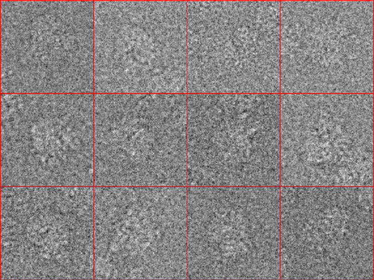
(a) Example of experimental images

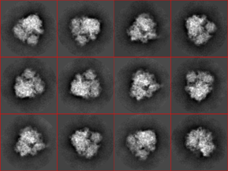
(b) Corresponding enhanced images

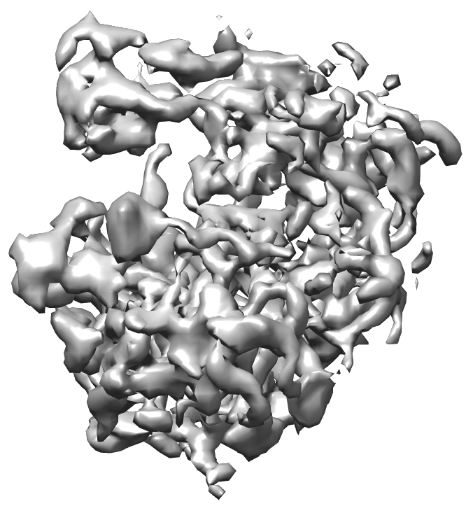
(c) Reconstructed volume

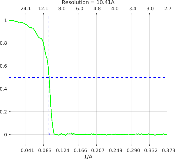
(d) FSC curve of the structure of panel (c)

Figure 1: EMPIAR 10028. The resolution of the reconstructed structure is 10.41Å

3.2 EMPIAR 10073

This data set of the yeast spliceosomal U4/U6.U5 tri-snRNP is available as the 10073 entry of EMPIAR (the corresponding entry in EMDB is EMD-8012) [23]. This data set contains 138840 images of size $380\times 380$. The nearest neighbor search took 2.5 minutes and producing 1500 class averages took roughly 100 minutes. The results are presented in Figure 2. The resolution of the reconstructed structure is 19.58 Å.

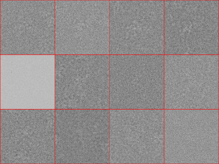
(a) Example of experimental images

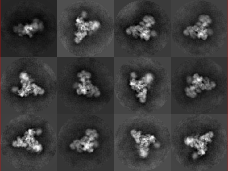
(b) Corresponding enhanced images

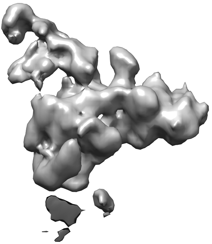
(c) Reconstructed volume

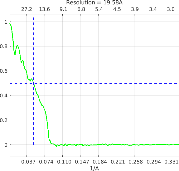
(d) FSC curve of the structure of panel (c)

Figure 2: EMPIAR 10073. The resolution of the reconstructed structure is 19.58Å

3.3 EMPIAR 10081

This data set of the human HCN1 hyperpolarization-activated cyclic nucleotide-gated ion channel is available as the 10081 entry of EMPIAR (the corresponding entry in EMDB is EMD-8511) [19]. This data set contains 55870 images of size $256\times 256$. The nearest neighbor search took less than 3 minutes and producing 1500 high-quality images took roughly 1 hour. Figure 3 shows the results. The resolution of the reconstructed structure is 11.25 Å.

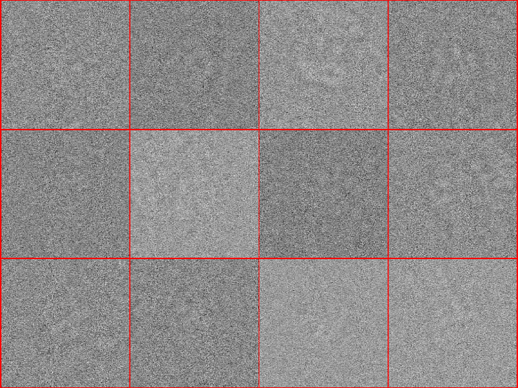
(a) Example of experimental images

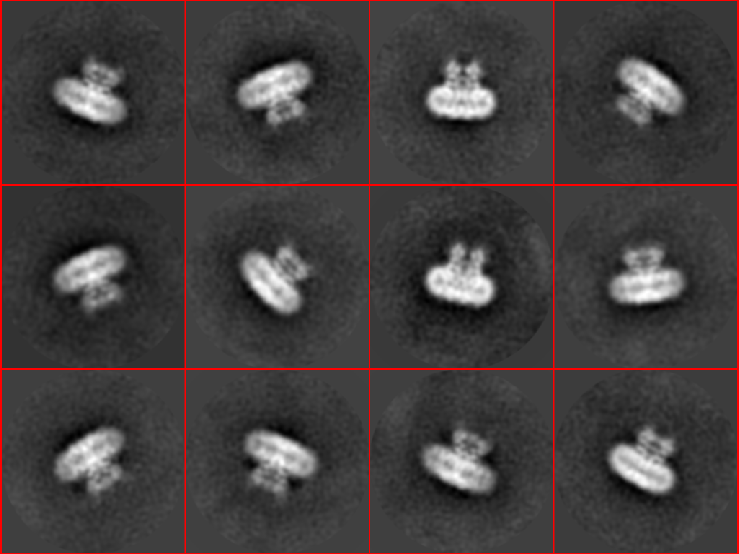
(b) Corresponding enhanced images

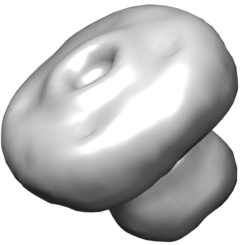
(c) Reconstructed volume

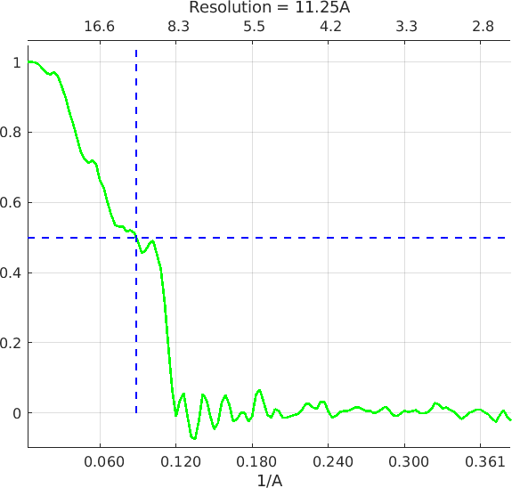
(d) FSC curve of the structure of panel (c)

Figure 3: EMPIAR 10081. The resolution of the reconstructed structure is 11.25Å

3.4 EMPIAR 10061

The next data set represents the structure of beta-galactosidase in complex with a cell-permeant inhibitor, available as the 10061 entry of EMPIAR (the corresponding entry in EMDB is EMD-2984) [3]. This data set contains 41123 images of size $768\times 768$ pixels. Figure 4 shows examples of raw data images, the corresponding enhanced images, and a 3-D structure reconstructed from the enhanced images using the spectral algorithm implemented in ASPIRE [25]. Although the class averages look of good quality, the resolution of the reconstructed structure is only 22.63 Å. The nearest neighbor search took less than 3 minutes and producing 1500 class averages took roughly 2.5 hours.

(a) Example of experimental images

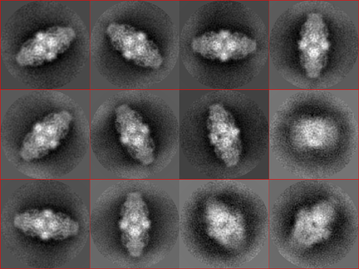
(b) Corresponding enhanced images

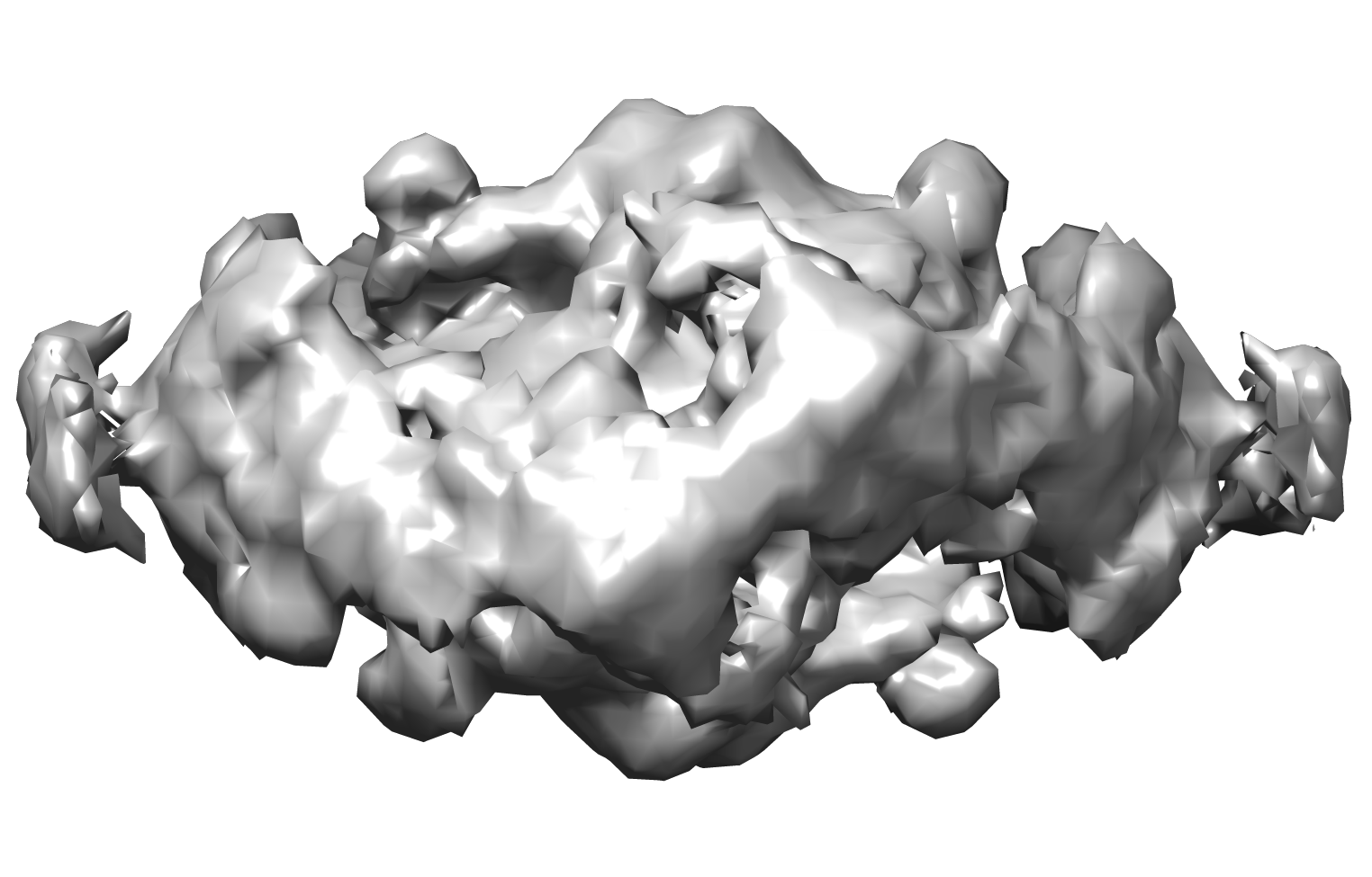
(c) Reconstructed volume

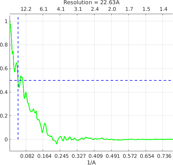
(d) FSC curve of the structure of panel (c)

Figure 4: EMPIAR 10061. The resolution of the reconstructed structure is 22.63Å

Table 1: Runtime

EMPIAR entry	# images	Dimensions	Preprocessing [sec]	sPCA [sec]	Nearest neighbor search [sec]	EM [sec]	Total [sec]
10028	105247	360x360	1032	1036	131	2299	4508
10073	138840	380x380	1735	1397	155	2735	6037
10081	55870	256x256	1405	698	170	1149	3427
10061	41123	768x768	2405	540	184	5261	8413

4 Discussion

In this paper, we have presented a new algorithm to enhance the quality of cryo-EM images, which can be used for various tasks in the computational pipeline of cryo-EM. The algorithm is based on [34], but extends it in several ways, which are crucial to improve its performance and to design built-in quality measures. The algorithm is computationally efficient and can be executed on large experimental data sets.

For larger data sets, the brute-force nearest neighbor search can be replaced by efficient randomized algorithms [16] with better asymptotic computational complexity. However, for contemporary data sets, the running time of both approaches is comparable. Our classification is approximately invariant under in-plane rotations and reflections; see also [10] for a related approach. While it can be extended to translation invariance by explicitly considering different translations, it will significantly increase the running time. A possible alternative approach would be to employ polynomials that are approximately invariant under the group of in-plain rotations and translations (namely, the group of rigid motions SE(2)) [7].

To improve the quality of the nearest neighbor search, the classes are refined by analyzing the spectrum of synchronization matrices. This provides a validation measure that can be computed directly from the data, which is crucial to mitigate the risk of model bias in downstream tasks, such as ab initio modeling. We have demonstrated that the enhanced images are of high quality so that they can be used to construct ab initio models. To cover all viewing angles, we randomly sample the data set. This is clearly not optimal, and we intend to study different deterministic strategies to sample the data.

References

- [1] ASPIRE: Algorithms for single particle reconstruction software package. http://spr.math.princeton.edu/.
- [2] Xiao-Chen Bai, Greg McMullan, and Sjors HW Scheres. How cryo-EM is revolutionizing structural biology. Trends in biochemical sciences, 40(1):49–57, 2015.
- [3] Alberto Bartesaghi, Alan Merk, Soojay Banerjee, Doreen Matthies, Xiongwu Wu, Jacqueline LS Milne, and Sriram Subramaniam. 2.2 Å resolution cryo-EM structure of -galactosidase in complex with a cell-permeant inhibitor. Science, 348(6239):1147–1151, 2015.
- [4] Tamir Bendory, Alberto Bartesaghi, and Amit Singer. Single-particle cryo-electron microscopy: Mathematical theory, computational challenges, and opportunities. IEEE signal processing magazine, 37(2):58–76, 2020.
- [5] Tamir Bendory, Nicolas Boumal, Chao Ma, Zhizhen Zhao, and Amit Singer. Bispectrum inversion with application to multireference alignment. IEEE Transactions on signal processing, 66(4):1037–1050, 2017.
- [6] Tamir Bendory, Dan Edidin, William Leeb, and Nir Sharon. Dihedral multi-reference alignment. IEEE Transactions on Information Theory, 68(5):3489–3499, 2022.
- [7] Tamir Bendory, Ido Hadi, and Nir Sharon. Compactification of the rigid motions group in image processing. SIAM Journal on Imaging Sciences, 15(3):1041–1078, 2022.
- [8] Tristan Bepler, Kotaro Kelley, Alex J Noble, and Bonnie Berger. Topaz-denoise: general deep denoising models for cryoEM and cryoET. Nature communications, 11(1):1–12, 2020.
- [9] Tejal Bhamre, Teng Zhang, and Amit Singer. Denoising and covariance estimation of single particle cryo-EM images. Journal of structural biology, 195(1):72–81, 2016.
- [10] Jameson Cahill, Joseph W Iverson, Dustin G Mixon, and Daniel Packer. Group-invariant max filtering. arXiv preprint arXiv:2205.14039, 2022.
- [11] Hongwei Cheng, Zydrunas Gimbutas, Per-Gunnar Martinsson, and Vladimir Rokhlin. On the compression of low rank matrices. SIAM Journal on Scientific Computing, 26(4):1389–1404, 2005.
- [12] Joachim Frank. Three-dimensional electron microscopy of macromolecular assemblies: visualization of biological molecules in their native state. Oxford university press, 2006.
- [13] Ido Greenberg and Yoel Shkolnisky. Common lines modeling for reference free ab-initio reconstruction in cryo-EM. Journal of structural biology, 200(2):106–117, 2017.
- [14] Richard Henderson. Avoiding the pitfalls of single particle cryo-electron microscopy: Einstein from noise. Proceedings of the National Academy of Sciences, 110(45):18037–18041, 2013.
- [15] Andrii Iudin, Paul K Korir, José Salavert-Torres, Gerard J Kleywegt, and Ardan Patwardhan. EMPIAR: a public archive for raw electron microscopy image data. Nature methods, 13(5):387–388, 2016.
- [16] Peter Wilcox Jones, Andrei Osipov, and Vladimir Rokhlin. Randomized approximate nearest neighbors algorithm. Proceedings of the National Academy of Sciences, 108(38):15679–15686, 2011.
- [17] Werner Kühlbrandt. The resolution revolution. Science, 343(6178):1443–1444, 2014.
- [18] Catherine L Lawson, Ardan Patwardhan, Matthew L Baker, Corey Hryc, Eduardo Sanz Garcia, Brian P Hudson, Ingvar Lagerstedt, Steven J Ludtke, Grigore Pintilie, Raul Sala, et al. EMDataBank unified data resource for 3DEM. Nucleic acids research, 44(D1):D396–D403, 2016.
- [19] Chia-Hsueh Lee and Roderick MacKinnon. Structures of the human HCN1 hyperpolarization-activated channel. Cell, 168(1-2):111–120, 2017.
- [20] Hongjia Li, Hui Zhang, Xiaohua Wan, Zhidong Yang, Chengmin Li, Jintao Li, Renmin Han, Ping Zhu, and Fa Zhang. Noise-Transfer2Clean: denoising cryo-EM images based on noise modeling and transfer. Bioinformatics, 38(7):2022–2029, 2022.
- [21] Dmitry Lyumkis. Challenges and opportunities in cryo-EM single-particle analysis. Journal of Biological Chemistry, 294(13):5181–5197, 2019.
- [22] Kazuyoshi Murata and Matthias Wolf. Cryo-electron microscopy for structural analysis of dynamic biological macromolecules. Biochimica et Biophysica Acta (BBA)-General Subjects, 1862(2):324–334, 2018.
- [23] Thi Hoang Duong Nguyen, Wojciech P Galej, Xiao-chen Bai, Chris Oubridge, Andrew J Newman, Sjors HW Scheres, and Kiyoshi Nagai. Cryo-EM structure of the yeast U4/U6. U5 tri-snRNP at 3.7 Å resolution. Nature, 530(7590):298–302, 2016.
- [24] Eugene Palovcak, Daniel Asarnow, Melody G Campbell, Zanlin Yu, and Yifan Cheng. Enhancing the signal-to-noise ratio and generating contrast for cryo-EM images with convolutional neural networks. IUCrJ, 7(6):1142–1150, 2020.
- [25] Eitan Rosen and Yoel Shkolnisky. Common lines ab initio reconstruction of D_2-symmetric molecules in cryo-electron microscopy. SIAM Journal on Imaging Sciences, 13(4):1898–1944, 2020.
- [26] Sjors HW Scheres. RELION: implementation of a Bayesian approach to cryo-EM structure determination. Journal of structural biology, 180(3):519–530, 2012.
- [27] Fred J Sigworth. A maximum-likelihood approach to single-particle image refinement. Journal of structural biology, 122(3):328–339, 1998.
- [28] Amit Singer. Angular synchronization by eigenvectors and semidefinite programming. Applied and computational harmonic analysis, 30(1):20–36, 2011.
- [29] Amit Singer and Yoel Shkolnisky. Three-dimensional structure determination from common lines in cryo-EM by eigenvectors and semidefinite programming. SIAM journal on imaging sciences, 4(2):543–572, 2011.
- [30] Amit Singer and Fred J Sigworth. Computational methods for single-particle electron cryomicroscopy. Annual Review of Biomedical Data Science, 3:163, 2020.
- [31] Carlos Oscar S Sorzano, JR Bilbao-Castro, Y Shkolnisky, M Alcorlo, R Melero, G Caffarena-Fernández, M Li, G Xu, R Marabini, and JM Carazo. A clustering approach to multireference alignment of single-particle projections in electron microscopy. Journal of structural biology, 171(2):197–206, 2010.
- [32] Wilson Wong, Xiao-chen Bai, Alan Brown, Israel S Fernandez, Eric Hanssen, Melanie Condron, Yan Hong Tan, Jake Baum, and Sjors HW Scheres. Cryo-EM structure of the plasmodium falciparum 80S ribosome bound to the anti-protozoan drug emetine. Elife, 3:e03080, 2014.
- [33] Zhizhen Zhao, Yoel Shkolnisky, and Amit Singer. Fast steerable principal component analysis. IEEE Transactions on Computational Imaging, 2(1):1–12, 2016.
- [34] Zhizhen Zhao and Amit Singer. Rotationally invariant image representation for viewing direction classification in cryo-EM. Journal of structural biology, 186(1):153–166, 2014.