Polarized Maser Emission with In-Source Faraday Rotation
Abstract
We discuss studies of polarization in astrophysical masers with particular emphasis on the case where the Zeeman splitting is small compared to the Doppler profile, resulting in a blend of the transitions between magnetic substates. A semi-classical theory of the molecular response is derived, and coupled to radiative transfer solutions for 1 and 2-beam linear masers, resulting in a set of non-linear, algebraic equations for elements of the molecular density matrix. The new code, PRISM, implements numerical methods to compute these solutions. Using PRISM, we demonstrate a smooth transfer between this case and that of wider splitting. For a J=1-0 system, with parameters based on the transition of SiO, we investigate the behaviour of linear and circular polarization as a function of the angle between the propagation axis and the magnetic field, and with the optical depth, or saturation state, of the model. We demonstrate how solutions are modified by the presence of Faraday rotation, generated by various abundances of free electrons, and that strong Faraday rotation leads to additional angles where Stokes-Q changes sign. We compare our results to a number of previous models, from the analytical limits derived by Goldreich, Keeley and Kwan in 1973, through computational results by W. Watson and co-authors, to the recent work by Lankhaar and Vlemmings in 2019. We find that our results are generally consistent with those of other authors given the differences of approach and the approximations made.
1 Introduction
Polarization in astrophysical masers has been one of the most controversial themes in the field, owing to a number of rival theories and further obfuscation due to different conventions regarding the definitions of right and left-handed polarized radiation, and the Stokes parameters that are widely used to describe intensity-like quantities. The early paper by Goldreich et al. (1973) (GKK) is still regarded as the seminal work in maser polarization theory, at least where this is based on Zeeman splitting of molecular transitions. It separates possible masers into a number of cases, based on the strength of the magnetic field and the degree of saturation, for example. Perhaps the most important limit, with regard to the present work, is the case where the magnetic field is strong enough to define a good quantization axis, but is adequate only to split the transition by a frequency much smaller than the Doppler width. It is in this case, where the Zeeman-split transitions form an overlapping group, that most controversy has arisen. GKK analysed this case in the limit of ultimate saturation, where the differentials of the Stokes parameters in the maser propagation equations tend to zero, and were able to obtain a set of analytical expressions for the Stokes parameters.
What GKK did not do was to analyse the overlapping group in the intermediate saturation regime. To do this, the differential equations describing maser amplification and saturation must be solved in a consistent manner all the way from negligible saturation to very high degrees of saturation. Numerical solutions covering the required range of saturation were computed in a series of papers involving the late W.D. Watson, beginning with Western & Watson (1984), which included models with two counter-propagating beams and both and Zeeman systems. An important result was that the GKK limits for strong saturation were approached rather slowly, and are the same for and groups. The model was later extended to include the effects of velocity gradients (Deguchi et al., 1986) and applied specifically to the 22-GHz maser transition of H2O (Deguchi & Watson, 1986). Further investigations found that a high polarization regime, originally investigated by GKK, where the stimulated emission rate, R, exceeds the Zeeman splitting, , but is vastly less than the square of the splitting divided by the loss rate, (i.e. ), applies only to the system. The usual restriction on the stimulated emission rate to be smaller than the Zeeman splitting was lifted (Nedoluha & Watson, 1990) by including off-diagonal elements of the density matrix that couple Zeeman substates of levels with the same value of : we will refer to these later as type 2 elements.
The early Watson models had boxcar line profiles and no spectral information, and could therefore not address the generation of circular polarization in the overlapping Zeeman case: Stokes is zero at line center, and antisymmetric about the center, so that a value of zero also results from a line profile average. Circular polarization and a spectral response were added in improved models that computed Stokes (Nedoluha & Watson, 1992, 1994). Anisotropic pumping, a feature of many numerical models since Western & Watson (1984) was favoured over Faraday depolarization for selective loss of Stokes and (Wallin & Watson, 1997). Maser polarization from unsaturated amplification through a turbulent velocity field driven by the rotation of an accretion disc was studied in Watson & Wiebe (2001). The work from this series on which we base most of our comparisons is Watson & Wyld (2001), which is based on the Nedoluha & Watson (1992) model, but includes calculations at many more angles of the magnetic field with respect to the radiation propagation axis, and a wider range of saturation levels. We note here that although the fundamental equations that we use are the same as those used in the Watson series, there are substantial differences in the methods of solution, so a primary purpose of the current work is to demonstrate that very similar results arise from these different methods. One important difference is that models in the Watson series are solved via a time-domain molecular polarization (for example eq.(11) of Nedoluha & Watson (1990)), followed presumably by a steady-state approximation to their eq.(4), whilst our method involves a formal Fourier transform to the frequency domain, where the combined density matrix and radiative transfer equations are solved: a spectral distribution is therefore fundamental to our model. Our method therefore has more in common with the methods used by Menegozzi & Lamb (1978) (no polarization) and Dinh-v-Trung (2009a) than with Watson and his co-workers. A second important difference is in the way in which the radiation transfer itself is treated: while the calculations in the Watson series are based on the solution of coupled ODEs, we make formal solutions of the transfer equations, reducing the problem to a set of non-linear algebraic equations in the inversions (see Section 3).
Another problem that bedevils polarisation work in general is that authors, over the years, have adopted several different conventions regarding definitions of left and right-handed waves, the definition of Stokes and the labeling of the helical transitions within the Zeeman pattern. Although most work is internally self-consistent, it is often confusing to relate it to the theoretical work of others, and to observational data. These problems are discussed in Green et al. (2014), where maser polarisation conventions are discussed in relation to observations of polarization in the 21-cm hydrogen line. We specify our conventions in Section 2.
1.1 Application to Observations
With regard to observational data, strong polarization is one of the characteristics of astrophysical masers, detected during the earliest work in the field (Weinreb et al., 1965). A good summary is Surcis et al. (2018). A distinction should be drawn between the paramagnetic molecules, for example OH, CH, in which much information can be gleaned directly from observations, and the closed shell species (for example H2O, SiO and CH3OH) in which more sophisticated analysis, including numerical modeling, is generally needed. In the former case, the magnitude of the magnetic field can typically be determined from the Zeeman splitting of lines, rather than their polarization, and the sense of the magnetic field (towards or away from the observer) can be determined from the handedness of elliptical polarization found in the lower-frequency member of a pair, for example Green et al. (2014). If linear polarization is present, the orientation of the magnetic field in the plane of the sky can be deduced, providing that a spectral component can be identified as a sigma or pi transition. Radiative transfer analysis is only required for a full 3D reconstruction of the vector magnetic field.
In the case of closed-shell molecules, the Zeeman splitting is much smaller than the Doppler line width, and numerical modeling is required to extract any useful information at all from polarization-sensitive observations. For example, direct observables, like the Stokes-I and Stokes-V spectral profiles need model fitting to recover the line-of-sight component of the magnetic field and further modeling to recover the full field strength, since the relation that the fractional circular polarization is proportional to breaks down for saturated masers (for example Vlemmings et al. 2006). The derived angle , between the magnetic field and the maser propagation direction, and the fractional linear polarization, may then be used to derive the level of saturation of the maser. Knowledge of can also be used to break the EVPA (electric vector position angle) degeneracy, determining the field as either parallel or perpendicular to the EVPA (Vlemmings et al., 2006). Small-scale (of order tens to hundreds of AU) variations in field structure can be traced if the field direction can be followed along imaged maser features. Examples of this include preferential alignment of the magnetic field with outflow axes in massive star-forming regions (Surcis et al., 2015), and the change in field orientation over a timescale of 7 yr in the VLA2 sub-source of W75N (Surcis et al., 2014).
Observations of SiO masers towards asymptotic giant branch (AGB) stars have revealed cases where the EVPA of linear polarization rotates through approximately within the apparent confines of a single maser object or cloud (Kemball et al., 2011; Assaf et al., 2013). Modeling of such EVPA rotations offers the possibility of distinguishing between the Zeeman interpretation of maser polarization and a number of competing theories (Tobin et al., 2019). The phenomenon may also be related to pulsation shocks emanating from the star and/or to the overall magnetic field structure of the circumstellar envelope that can be tested through additional models, for example Pascoli & Lahoche (2010); Pascoli (2020).
2 Saturation model
Our model is derived through the following key stages: First, the time-dependent Schrödinger equation is solved via an expansion of the wavefunction in a basis set of the eigenfunctions (the energy levels) of the corresponding time-independent equation. Products of the coefficients of this expansion, averaged over a volume of order , where is a typical maser wavelength, become elements of the density matrix (DM). This solution is facilitated by a separation of the Hamiltonian operator into a time-independent component and a time-dependent interaction component that is a function of the electric field that drives transitions between the energy levels. If this interaction operator is further split into a coherence-preserving component, based on the electric field of the maser, and another component containing all other (‘kinetic’) processes, then the solution of the original Schrödinger equation reduces to solving a pair of differential equations for elements of the DM: one for diagonal elements, where the energy-level indices of the element are equal, and one for off-diagonal elements, where they are not. With a little more work, diagonal elements may be paired, resulting in equations for the inversion between pairs of levels. The resulting ‘optical Bloch equations’ may be written,
| (1) |
for the off-diagonal DM element, , representing coherence between levels and , and
| (2) |
for the population inversion, , between these levels. All DM elements are functions of time, , position, and Doppler velocity, . The index runs over the energy levels in the model, and angular frequencies of the transitions between them are written . The maser part of the interaction hamiltonian, linking levels and , is represented as . As matrices, both the interaction hamiltonian and the DM are hermitian. The symbol denotes taking the imaginary part. Coherence between levels is lost at the rate , which encompasses all elastic and inelastic collisions, and radiative processes that are not stimulated emission across the maser levels. is the loss rate to the inversion, and so represents a subset of those processes contributing to , since elastic processes are excluded. A phenomenological pump rate per unit volume, , is included to support the inversion. The pumping term contains the normalised gaussian function with width parameter,
| (3) |
where is Boltzmann’s constant, is the kinetic temperature in the maser zone and is the molecular mass of the maser species. We assume negligible velocity redistribution (NVR), so that population is not exchanged between different velocity subgroups of the DM. This approximation also implies that .
The maser part of the interaction hamiltonian is defined as
| (4) |
where is the molecular dipole operator for the transition, and is the electric field of the maser radiation. In the case of Zeeman-based maser polarization, we do not assign the electric field to a particular transition, since the response of several transitions may overlap in frequency. The electric field is the real part of the complex analytic signal . From this point, we consider propagation only along the -axis, so that the analytic signal appears as
| (5) |
for propagation in the positive direction, where and are the and components, respectively, of the time-domain complex amplitude of the field. We consider a broad-band electric field, and this may be written decomposed into its Fourier components of width , where is a finite sampling time. In the Fourier representation,
| (6) |
where is the angular frequency of the th Fourier component and and are the components of the field amplitude at that frequency.
Our conventions regarding the electric field are the following: we adopt the IEEE definition of a right-handed wave (IEEE-STD-145 of 1993) and the IAU axis system, in which the axis points towards the observer, the axis towards North and the axis, East (Hamaker & Bregman, 1996; van Straten et al., 2010). We also use the IAU definition of Stokes as the right-handed intensity minus the left-handed intensity. We use the naming convention of Garcia-Barreto et al. (1988) for Zeeman-split transitions, so that, for a molecule that has Landé factors with the same sign as OH, the transition has the lowest frequency in a triplet, and changes magnetic quantum number by in emission.
The second key stage is the application of a rotating wave approximation that eliminates all terms oscillating at frequencies corresponding to the band-centre frequency of the radiation. To this end, the Fourier frequencies in eq.(6) are expanded as , where is the band-center frequency and is a local frequency, measured from , and is never larger than a few Doppler widths.
The third stage is to apply a time-to-(angular) frequency Fourier transform of the time-domain DM equations (Menegozzi & Lamb, 1978; Dinh-v-Trung, 2009a). The result is a set of non-linear algebraic equations in the Fourier components of the inversions and of the slow part of the off-diagonal DM equations. These equations also contain Fourier components of the electric field complex amplitudes.
At this point, we restrict our analysis to the case where there is just one transition of each helical type, which requires both unsplit maser levels to have the same Landé splitting factor. We do this because the numerical calculations in the present work apply to the Zeeman-split transition of SiO. More general cases have Zeeman energy shifts that are different in the upper and lower unsplit states, for example eq.(9.1) of Gray (2012). In this case there can be several transitions of each helical type when the external magnetic field is applied, and these have different line strengths in general. The formalism of a single transition each of , and type can be restored by employing the averaged Landé splitting factor for one group of transitions (by symmetry the average for the transitions is zero). See, for example Landi Degl’Innocenti & Landolfi (2004).
Dipole operators that are pure right- or left-handed for the respective and Zeeman transitions, or lie along the -axis for transitions in a frame where the magnetic field is , have been rotated into a frame where the radiation propagates along the axis. To allow for Faraday rotation, the axis is constrained to lie in the plane, but may be offset by an angle from the axis. The angle is the offset between the and axes.
The slow off-diagonal DM elements are then either
| (7) |
for transitions, where superscripts denote the transition type, and subscripts , or combinations thereof, label the Fourier components. The electric field amplitudes in eq.(7) are in the circular polarization basis, with denoting right and left-handed polarization, respectively. The symbol denotes a complex lorentzian function. For transitions, identified by the zero superscript,
| (8) |
The inversions, and are now also labeled by Fourier component, or population pulsation, , in the and transitions. We note that the inversion in the central Fourier component, is real, but the other pulsations are complex in general. Fourier components of the inversion are given by the diagonal DM equations,
| (9) |
for the transitions, where , is the Kronecker delta and
| (10) |
for transitions.
Further operations carried out on eq.(9) and eq.(10), and the definitions of the complex lorentzian functions, and are deferred to Appendix A. The results of these operations are the key equations for the molecular response as a function of angular frequency,
| (11) |
for the transitions and
| (12) |
for the transition, noting that molecular responses are now saturated by Stokes parameters at specified frequencies. The index denotes a shift in frequency bins corresponding to the Zeeman splitting. We derive expressions in the following section that allow us to eliminate the Stokes parameters from eq.(11) and eq.(12).
3 Radiative transfer solution
At this point, our treatment departs significantly from most earlier work on maser polarization: instead of solving a set of differential radiative transfer equations in the Stokes parameters, we generate instead a formal solution of the transfer equation and eliminate the Stokes parameters, to leave only a set of algebraic equations in the elements of the DM.
In scalar radiative transfer problems, the elimination of the radiation intensity is one of the oldest methods of solving the combined radiative transfer and non-LTE statistical balance problem, for example Chandrasekhar (1950); King & Florance (1964), and is useful because it reduces the problem to a set of non-linear algebraic equations in the molecular populations or inversions only, obviating the need to compute any radiation integrals. The method was introduced in a modern context for the classic slab geometry by Elitzur & Asensio Ramos (2006), and has been used successfully for masers in a 3D finite-element model of maser clouds (Gray et al., 2018, 2019, 2020).
The additional problem, in the context of the present work, is that the standard method of writing a formal solution of the radiative transfer equation via the integrating factor method is not obviously applicable to the vector-matrix radiative transfer equation,
| (13) |
required to propagate polarized radiation along ray .
To obtain a formal solution of eq.(13) with the Stokes vector, , as the subject, we have adopted the operator method proposed by Landi Degl’Innocenti (1987). Following this method, the solution of eq.(13) is
| (14) |
for moving from ray position to position , where the evolution operator is the matrix,
| (15) |
where is the identity matrix. Note that the operator in eq.(15) differs from a standard exponential because of the presence of , the ‘chronological’ operator, that specifies the order in which the various gain matrices, the , must be multiplied.
The gain matrices used in the present work are the sum of a continuum version, containing only the Faraday rotation elements, and a line version, containing all the others. The combined gain matrix is
| (20) |
where the individual elements are defined as (Landi Degl’Innocenti, 1976; Landolfi & Landi Degl’Innocenti, 1982; Rees, 1987)
| (21) | ||||
| (22) | ||||
| (23) | ||||
| (24) | ||||
| (25) |
In the Faraday term, eq. (25), is the number density of free electrons, is the electron rest mass and is the band-center frequency of the maser radiation. We neglect continuum processes that would convert between linear and circular polarization.
We now note that if the evolution operator is eliminated from eq.(14), with the aid of eq.(15), a formal solution of the form,
| (26) |
is obtained, where the right-hand side is independent of the Stokes parameters except for background values where radiation enters the maser zone. For the case of an unpolarized background, , where is a background specific intensity. Furthermore, from the expressions in eq.(21)-eq.(24), we see that elimination of the Stokes parameters from eq.(11) and eq.(12) leads to a set of integral equations in the molecular responses at a particular position in the maser column. When the integrals are replaced by finite sums for numerical work, these equations become sets of non-linear algebraic equations involving molecular responses at, in principal, all positions, but no variable radiation intensities.
In order to make the non-linear algebraic equations suitable for numerical solution, eq.(11) and eq.(12) were reduced to the respective dimensionless forms,
| (27) |
and
| (28) |
where is the Doppler width ( in velocity units) converted to angular frequency. The lower case Stokes parameters are scaled to the saturation intensity, assumed here to be the same for all three helical transitions, and equal to,
| (29) |
where is the loss rate and and are the rest wavelength and Einstein A-value of the -transition. The dimensionless Stokes parameters are eliminated from eq.(11) and eq.(12) with the help of scaled versions of eq.(26) in which distances are scaled to an optical depth , defined as
| (30) |
Molecular responses have been scaled according to
| (31) |
in the process of converting eq.(11) (eq.(12)) to eq.(27) (eq.(28)). Other dimensionless parameters appearing in eq.(27) and eq.(28) are the relative pump rates in and transitions, and , the corresponding relative line strengths. When applied to eq.(21)-eq.(24) the scalings in eq.(29)-eq(31) result in the gain matrix elements
| (32) | ||||
| (33) | ||||
| (34) | ||||
| (35) |
The Faraday term behaves differently because it is a continuum, rather than a line, effect, and the dimensionless form of eq.(25) is
| (36) |
Finally, we note here that we opt not to convert the angular frequencies, and , to dimensionless values, to allow more direct control over selected angular frequency resolution, Doppler, and Zeeman widths in the numerical solver described below.
4 The numerical solver
We now discuss the numerical implementation of the one-dimensional formalism derived in the previous section. Functionally, the formalism comprised of eq.(27)-(28) and (32)-(36) forms a closed system of equations that is solved iteratively to calculate the Stokes parameters and corresponding population inversion for a given set of conditions.
In practice, according to eq.(26), the solution at any position along a line of sight through the cloud depends on the solution at every other point through which the ray has already traveled. In addition, the unitless inversions (eq.(27) and (28)) at any given frequency also depend on the solutions at frequencies . Therefore, the system of equations must be solved simultaneously at each frequency and optical depth through the masing material. However, they are fully separable along other parameters.
The one-dimensional radiative transfer solutions and their associated observables were computed with PRISM111github.com/tltobin/prism (Polarized Radiation Intensity from Saturated Masers; Tobin et al. 2022). PRISM, in its current form, was developed from an original code described in Tobin (2019). PRISM solves the dimensionless system of equations presented in the previous section simultaneously across a 2-dimensional grid of angular frequency, , and optical depth, , up to a given total optical depth for the cloud, . The numerical solution for the dimensionless inversions, is derived for each set of parameters using SciPy’s optimize.newton_krylov zero-finder. The residual between the starting for each iteration and the resulting value defined by eq.(27) and (28) is adjustable in PRISM; however, for all numerical solutions presented here, the tolerance for the solution at each grid point was set at .
The remaining parameters – , , , , , , the number of expansion terms used for eq.(26), , and the dimensionless background Stokes parameters, – are treated as constant throughout the cloud for a given solution. Faraday rotation can be included by either explicitly specifying a non-zero or by calculating it from eq.(36). In addition, PRISM can solve systems with either a single ray travelling in one direction or two opposing rays travelling in opposite directions through the one-dimensional cloud. The modifications to the formalism presented in the previous section that are required for the case of counter-propagating rays are detailed in Appendix B. In the case of counter-propagating rays, PRISM does not require the background Stokes parameters for the second ray to be identical to those of the first ray.
In practice, solving the system of equations iteratively at all grid points in space with an -fold expansion of integrated gain matrices can be time consuming, particularly as the total increases. To alleviate this concern, solutions are calculated for a given system for gradually increasing total optical depth. The calculation of at each subsequent total optical depth uses the solution for the previous total optical depth as its initial guess. In the numerical solutions presented here, we begin with a total optical depth of , which typically converges to within tolerance in only a few iterations of the newton_krylov solver.
While the method above is built directly into the PRISM code, other techniques may be required to speed convergence, particularly in cases where between successive iterations. In the case of large differences between in successive iterations, intermediate steps in with less stringent tolerances for convergence (eg. instead of ) may provide a more accurate initial guess for the next desired solution, despite the additional derivations.
Another time-saving option is to derive the solution at all desired using the method above at a single , and then use the solution as the initial guess for deriving the solution, provided that the step between and is small enough. With the sampling used in following sections ( for , for ), this method typically provides an improvement of several magnitudes in the initial residual for each new solution, and does not require the addition of intermediate . However, this method does require solutions at a single to already exist for any desired . Therefore, the method of choice when performing the work presented here for a set of solutions as a function of is to first compute solutions as a function of increasing for and individually, using intermediate as needed. These results are then used as anchors to calculate new solutions for desired only as increases from and decreases from . Once a population solution has been obtained in the space, computationally cheap formal solutions recover the Stokes parameters from eq.(13) and appropriate radiation boundary conditions.
When calculating the dimensionless Stokes parameters, , following eq.(26), the number of expansion terms required to converge on a solution to some desired precision increases substantially with and . However, the convergence of a solution also depends on other parameters, such as , to a lesser extent. The convergence for each solution is evaluated after calculation, to ensure that the desired precision was reached. Convergence is characterized for each full solution via a two-fold analysis of the absolute value of the expansion terms in eq.(26). For each solution grid calculated as a function of angular frequency from line center, , and optical depth through the cloud, , we calculate the maximum fractional contribution to each Stokes parameter from the th expansion term across all bins, or max. We then verify the results for a converging trend as the number of expansion terms, , increases. The convergence of a suite of solutions across and total optical depth, , are then characterized according to the maximum fractional contribution to a Stokes parameter for any at the final utilized expansion term for the highest total optical depth.
5 Results
5.1 Large and Small Zeeman Splitting Solutions
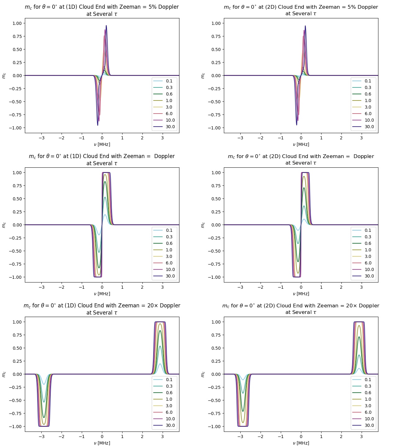
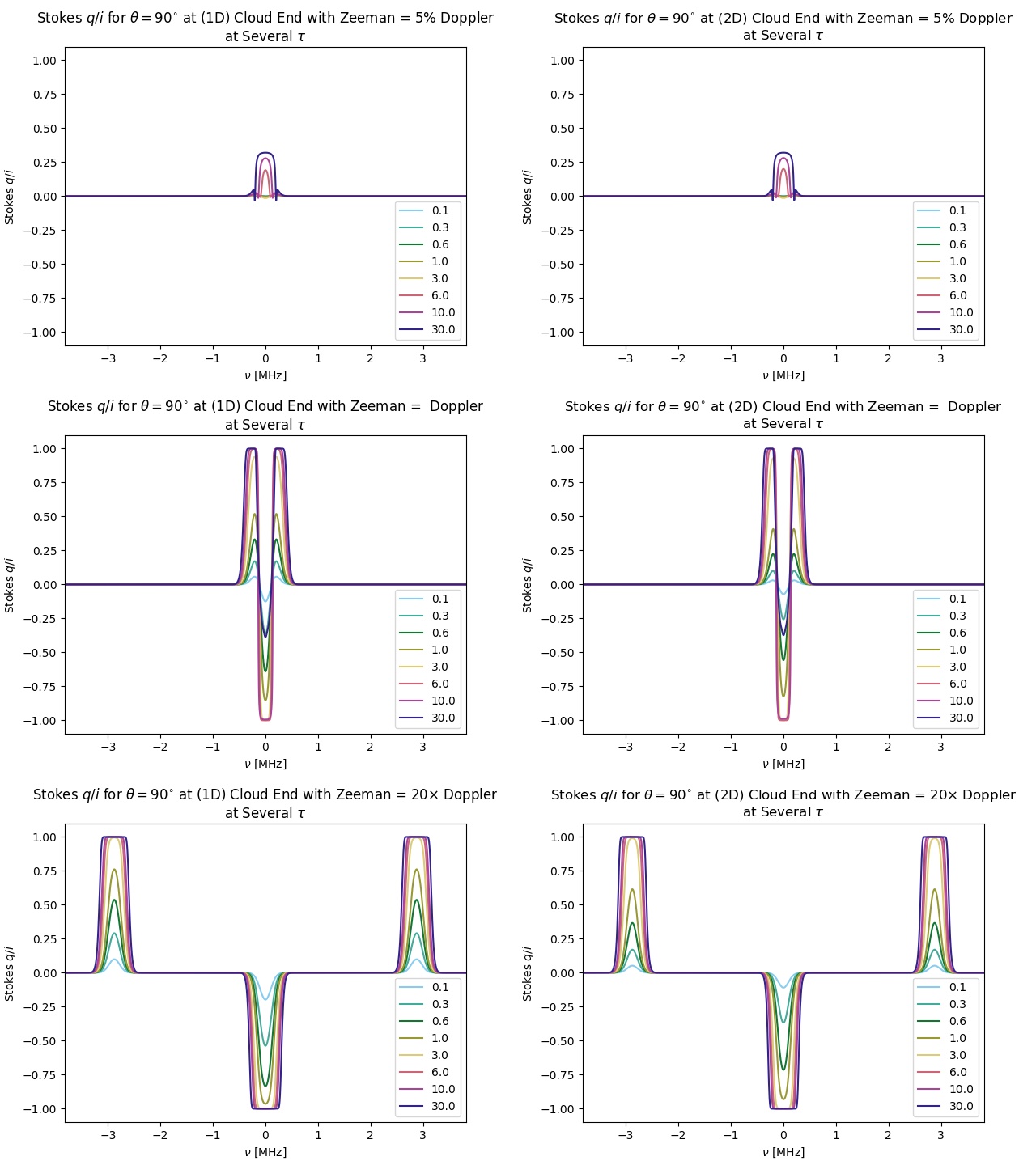
Although most of the results discussed in this work will focus on small Zeeman splitting at the level of SiO, the lack of assumptions about the strength of Zeeman splitting relative to the Doppler width in deriving the formalism provides a general formulation applicable to different molecular species. To demonstrate this, we derived solutions for the cases of a magnetic field parallel () and perpendicular () to the line of sight for uni-directional and bi-directional clouds. Using a Doppler width of s-1 (SiO , ; Boboltz & Diamond 2005; Lovas 2004), we vary the Zeeman splitting via , calculating a solution for a Zeeman shift of for total optical depths, , from . All used with expansion terms, for simplicity, and had a 5001 resolution elements along covering the range , with 101 resolution elements along .
The resulting fractional circular polarization () profiles with and linear polarization () profiles with at the end of the cloud are shown in Figures 1 and 2, respectively, for several representative . Most notably, for large Zeeman splitting (eg. ), the polarization profile for and approaches the solution for the normal longitudinal and transverse Zeeman effect, respectively. In these cases, the center of each component reaches 100% polarization at a total optical depth, , between 3 and 6.
| Parameter | Description | Value |
|---|---|---|
| Line Center Frequency | 43.122 GHz | |
| Doppler Width [Angular Frequency] | s-1 | |
| Doppler Width [velocity]aaOnly used for cases with nonzero Faraday rotation . | 997.8 m s-1 | |
| Single Substate Zeeman Splitting [Angular Frequency] | 740.48 ( B / 1 G ) s-1 | |
| Sky-plane angle | ||
| Squared Substate Dipole Moment Ratio | 1ggThis must be 1.0 for the present system; we leave it as a parameter to allow for future work with more complicated Zeeman patterns. | |
| Substate Pumping Rate Ratio | 1 | |
| Initial Unitless Stokes (,,,)bbFor bi-directional integration, the same initial Stokes are used for each ray. | (, 0, 0, 0) | |
| Loss RateaaOnly used for cases with nonzero Faraday rotation . | 5 s-1 | |
| Einstein A CoefficientaaOnly used for cases with nonzero Faraday rotation . | s-1 | |
| Pump Rate per Volume into 0 SubstateaaOnly used for cases with nonzero Faraday rotation . | cm-3 s-1 | |
| Sampled Angular Frequency | 740.48 s-1 | |
| L.o.S. Optical Depth Resolution | ||
| Angle between and L.o.S. | ||
| Magnetic Field Strength | GccB 2 G only used for uni-directional integration with no Faraday Rotation ( cm-3). | |
| Zeeman Splitting in Ang. Freq. Bins | ccB 2 G only used for uni-directional integration with no Faraday Rotation ( cm-3). | |
| Electron Number DensityddUsed to turn on/off Faraday Rotation. An cm-3 yields a . | cm-3,eeSolutions only computed with cm-3 for uni-directional clouds. | |
| Total Optical Depth | ffSolutions computed with cm-3 are only integrated up to maximum for B G, respectively. | |
| Number of Expansion Terms | 50 for cm-3 or ( B = 1 G, ) | |
| 70 for ( B = 5 G, ) | ||
| 80 for ( B = 10 G, ) | ||
| 100 for ( B = 1 G, ) | ||
| 110 for ( B = 5 G, ) | ||
| 120 for ( B = 10 G, ) |
5.2 SiO Polarization with No Faraday Rotation
We consider next the case of the SiO , transition as a function of for a range of total optical depths, , and magnetic field strengths. For the moment, we ignore Faraday Rotation by setting . We again use a Doppler width of with a line center frequency of 43.122 GHz (Boboltz & Diamond, 2005; Lovas, 2004). The angular frequency shift with respect to line center due to Zeeman splitting is given by (Pérez-Sánchez & Vlemmings, 2013). The latter is implemented by setting the angular frequency array as , and selecting [G]. As before, we use a resolution of 101 elements along for each calculation and 50 expansion terms. We also set for simplicity.
We compute a suite of uni-directional solutions in the cases of 1, 2, 5, and 10, corresponding to magnetic field strengths of 1 G, 2 G, 5 G, and 10 G, respectively. Within each solution, varies from and ranges from . Within this grid, increases in steps of through , followed by steps of thereafter; the exception is the solution, which is replaced by solutions at and for increased resolution around the Van Vleck angle (GKK). Solutions were computed for optical depths of 0.1, 0.3, 0.6, (1.0 - 3.0 in steps of 0.1), 4.5, 6, 8, 10, 13, 16, 20, 25, 30, 45, 60, 80, 100 . We compute a similar set of bidirectional solutions for 1 G, 5 G, and 10 G magnetic fields. We used expansion terms in all cases, achieving a precision of max at all sampled optical depths. A summary of the parameters used to derive the solutions described in this and following sections is shown in Table 1.
The behavior of the scaled intensity, , is similar across all cases. For a given optical depth and number of rays, changes little from - , decreasing slightly () as approaches . While there is no significant change in with , increasing the number of rays from one to two decreases the total by about a factor of 2. In the cases discussed here, the maximum reached for is for a uni-directional maser and for a bi-directional maser.
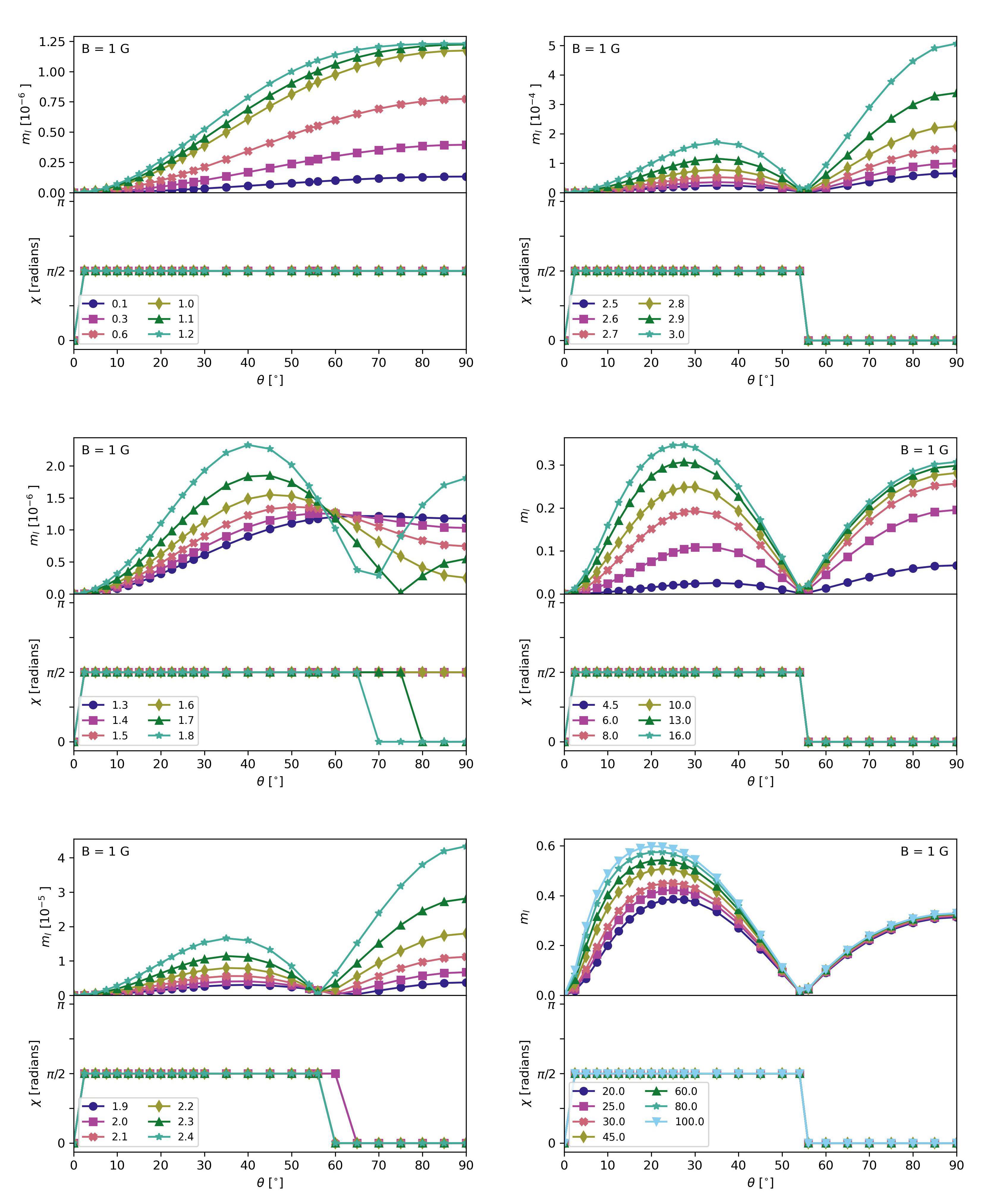
The resulting fractional linear polarization () and its position angle (EVPA) at line center for a one-directional maser in a 1 G magnetic field are shown in Figure 3 as a function of for all sampled . At this magnetic field strength, is low () for up to , increasing for larger and showing no flip in EVPA. We show in Appendix C that no flip is expected for negligible saturation. As increases further (), at higher begins to decrease even as it continues to increase at , forming a singularly-peaked function.
The EVPA flip appears first at , but at , while at larger than the flip location increases once again to form half of a second peak. As continues to increase up to , the at which the EVPA flip occurs approaches its final location between and ; meanwhile, increases in both peaks, though at quickly surpasses the peak at more moderate .
By , the EVPA flip has reached the Van Vleck angle to our resolution, where it stays for all remaining . The in both peaks continues to grow, with the peak at moderate finally reaching and surpassing that at around , when at both peaks. From there, continues to increase in the lower peak, with only slight increases in the of the peak.
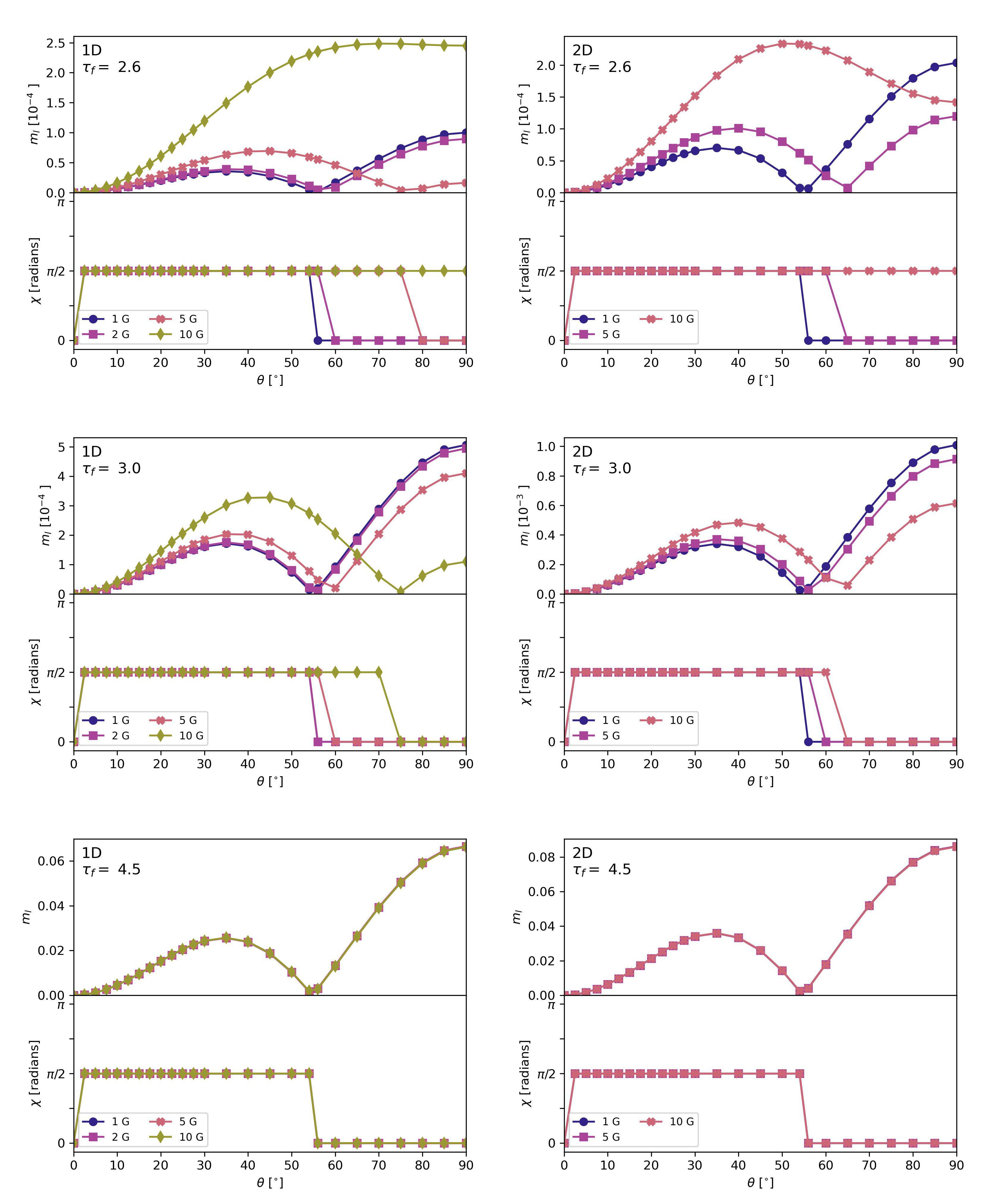
As shown in Figure 4, increasing the magnetic field strength increases both the scale of the fractional linear polarization present and the total optical depth, , required for the appearance of the EVPA flip and its approach to the Van Vleck angle. A comparison to the bi-directional cases shows that increasing from one to two rays causes the overall scale of to increase more quickly with , in addition to requiring lower for the appearance of the EVPA flip and its approach of the Van Vleck angle for a given magnetic field strength.
However, by , the EVPA flip occurs between and in all cases and no longer varies significantly with B. For an optical depth of , the largest difference in at line center between a 1 G and a 10 G magnetic field is for one-directional propagation and for bi-directional propagation. Compared to the peak values of 0.60 and 0.74, respectively, the variation from magnetic field strength alone is not visible to the eye when plotting at these high optical depths.
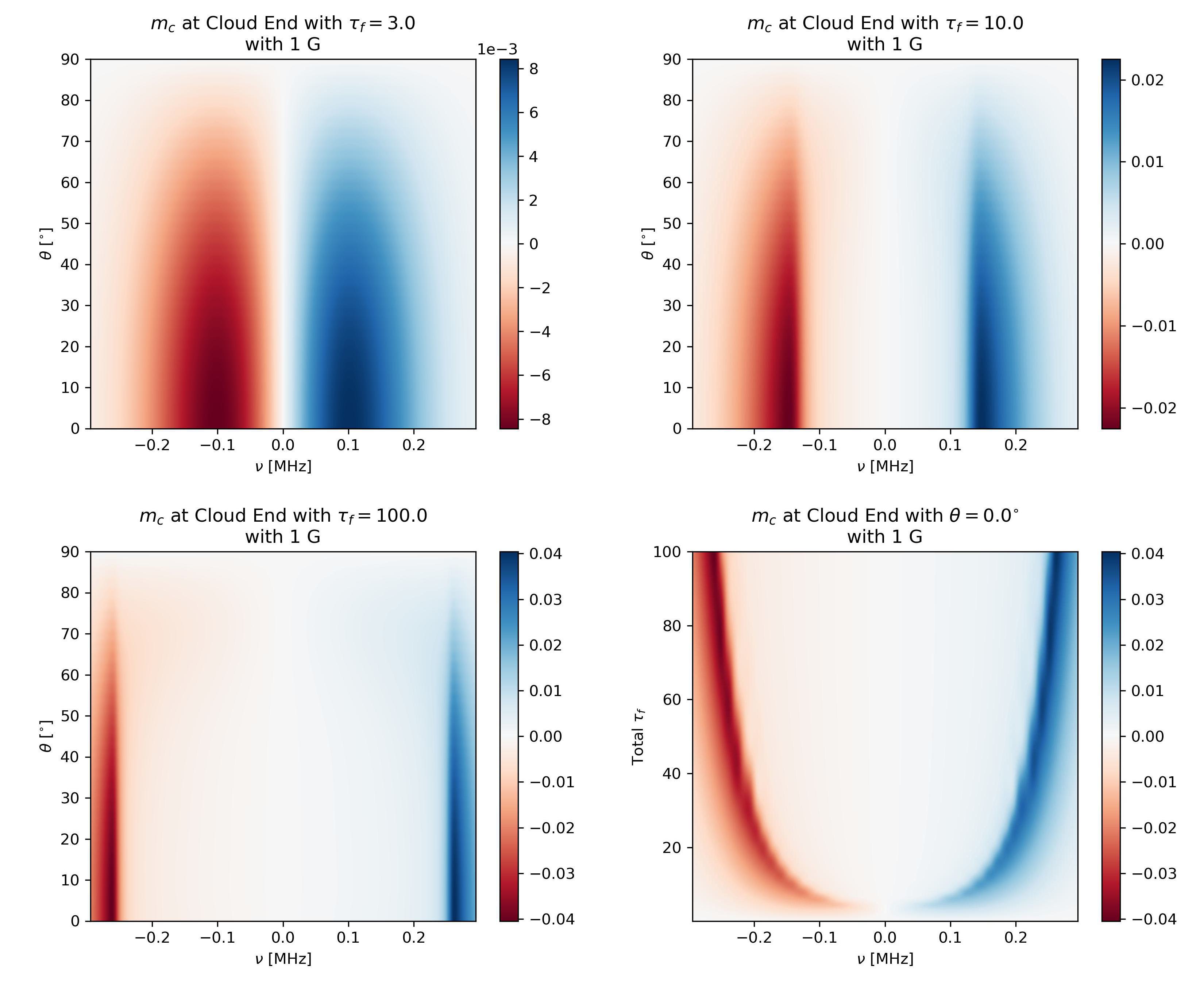
The circular polarization profile is antisymmetric about line center, resulting in at line center itself (see Figure 5). The maximum for a system at cloud end increases for larger values of and . For , the frequency at which the extrema occur ( kHz or ) is constant with and within the precision of our frequency resolution. For , the offset frequencies of the extrema increase approximately logarithmically with , reaching ( kHz) for . These higher optical depths also show a smaller dependence on , with the extrema for occurring s-1 ( ) further from line center at than the extrema with . However, this amounts to a change in frequency across all at a given optical depth, indicating that this effect is several orders of magnitude weaker than the change in peak frequency with .
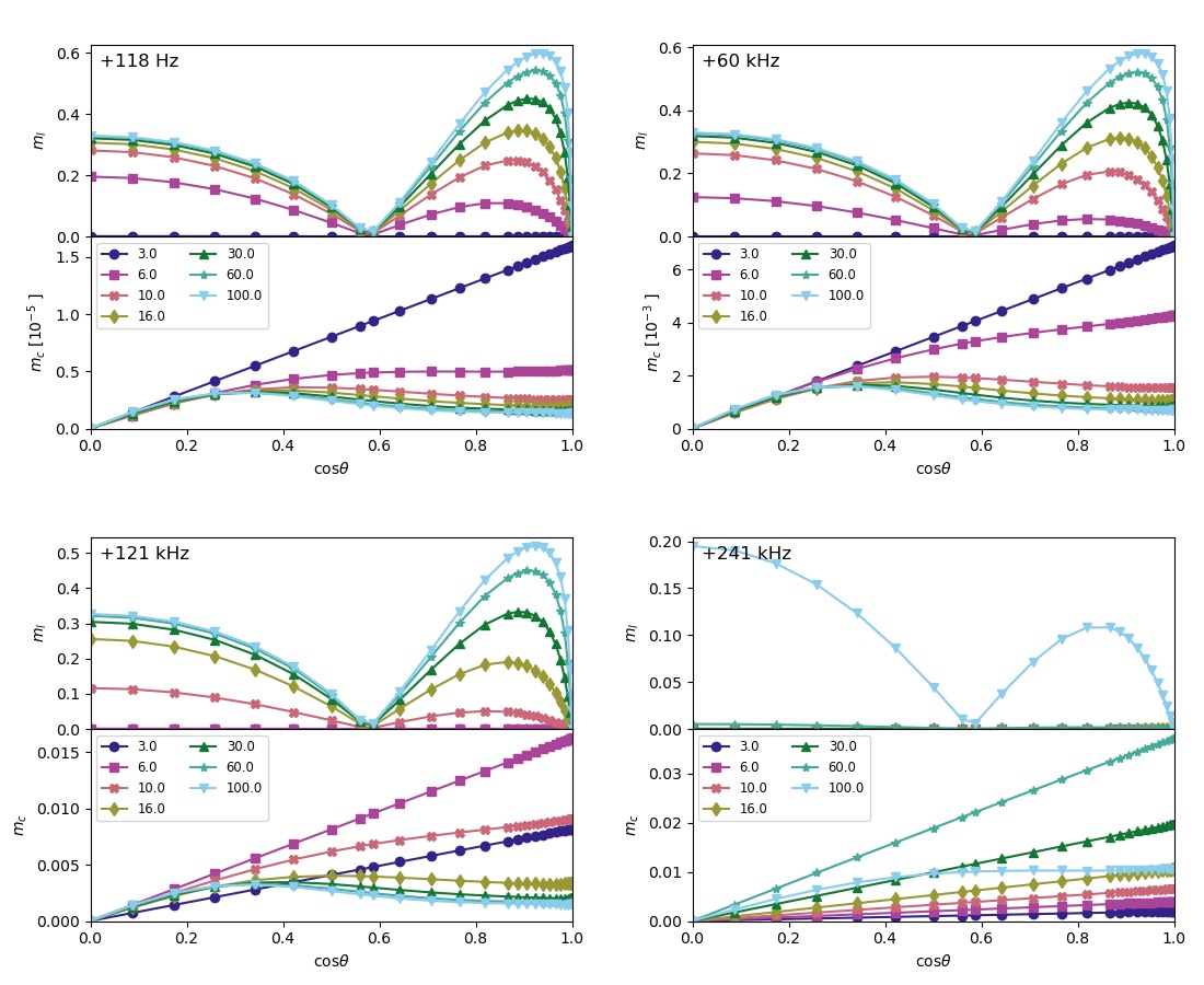
Figure 6 shows the and corresponding as a function of at +118 Hz, +60 kHz, +121 kHz, and +241 kHz from line center for between 3 and 100. In all cases, at ; i.e. no circular polarization arises when the magnetic field is oriented perpendicular to the line of sight. For , for all , with increasing with for a given . For , is only linear with at or outside of the peak frequencies. For frequencies interior to the peaks, deviates from linearity with , showing a greater decrease in at larger .
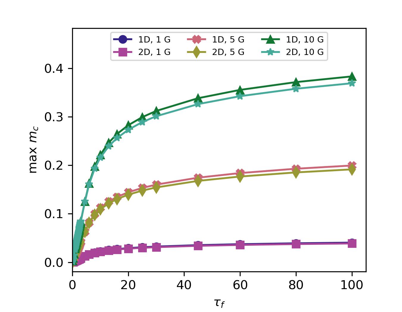
A uni-directional cloud with a 1 G magnetic field reaches a maximum fractional circular polarization of by (). It requires to achieve a peak and a for a peak with our frequency resolution. Figure 7 shows how the increase in maximum with varies with magnetic field strength and number of propagating rays. The increase in maximum with magnetic field strength is nearly proportional to the magnetic field strength, with a deviation from proportionality for up to 100. Calculating propagation with bi-directional rays instead of a single ray causes a peak for a given magnetic field, with values leveling out at for . However, notably, as seen in Figure 6, the larger frequency offsets from line center that provide of one to a few percent have lower linear polarization than at frequencies close to line center.
5.3 SiO polarization with nonzero Faraday rotation
We next consider similar cases with non-zero Faraday Rotation as set by eq.(36). We maintain the line center frequency, , of 43.122 GHz for the SiO , transition. The Doppler width in velocity space, , is calculated explicitly as , for consistency with the set Doppler width s-1. The decay or loss rate, , is estimated at s-1 (Kwan & Scoville, 1974; Nedoluha & Watson, 1990; Elitzur, 1992). The Einstein-A coefficient, , for the 28SiO , line is set at s-1 (Schöier et al., 2005), and the pump rate (per volume) into the 0 substate, , is derived from , where is the number density of SiO molecules and is the overall pump rate. For an cm-3 (Elitzur, 1992) and s-1 (Assaf et al., 2013) in the SiO masing environments around late-type evolved stars, we estimate a pump rate per volume of cm-3 s-1.
The electron number density, , in the near circumstellar environments of late-type evolved stars is not strongly constrained and can vary significantly within the region. While it can be derived simply from the number density of Hydrogen, , and the ionization fraction, , estimates of the ionization fraction in SiO masing regions around AGB stars range from (Reid & Menten, 1997) to (Gustafsson & Höfner, 2004). The models of Ireland et al. (2011) have a mean at , resulting in cm-3, assuming the relative H2/He abundances from Wong et al. (2016); however, the precise value of can very by 2 orders of magnitude in either direction depending on the modelled system and sampling time. This is consistent with the upper limit of cm-3 from Wong et al. (2016). Combined with the range of estimated above, this estimate of would indicate typical values of between cm-3 and cm-3.
We compute a grid of unidirectional solutions for each combination of cm-3 and 1, 5, 10 G. This, combined with the remaining estimated values above, gives us sampled 0.0193, 0.0965, 0.193, 0.386, 1.93, 3.86 . We also calculate the bi-directional solutions for the 7.85e3 cm-3 cases.
Increasing the Faraday Rotation via requires an increase in the number of expansion terms required to achieve the desired precision. The number of expansion terms, ranging from , are shown in Table 1. Solutions calculated with 7.85e3 cm-3 reach a precision of max for uni-directional clouds and for bi-directional clouds out to a total optical depth of 100. Solutions using 7.85e3 cm-3 were only computed up to total optical depths of for G, respectively. Although convergences at these maximum optical depth reached max, higher total optical depths resulted in either a significantly degraded convergence evaluated from the expansion term contributions or a failure to converge within the Newton Krylov solver. This behavior may be due to the increased Faraday Rotation generating structure in the Stokes parameters across the grid that is too fine for our grid resolution to sample smoothly.
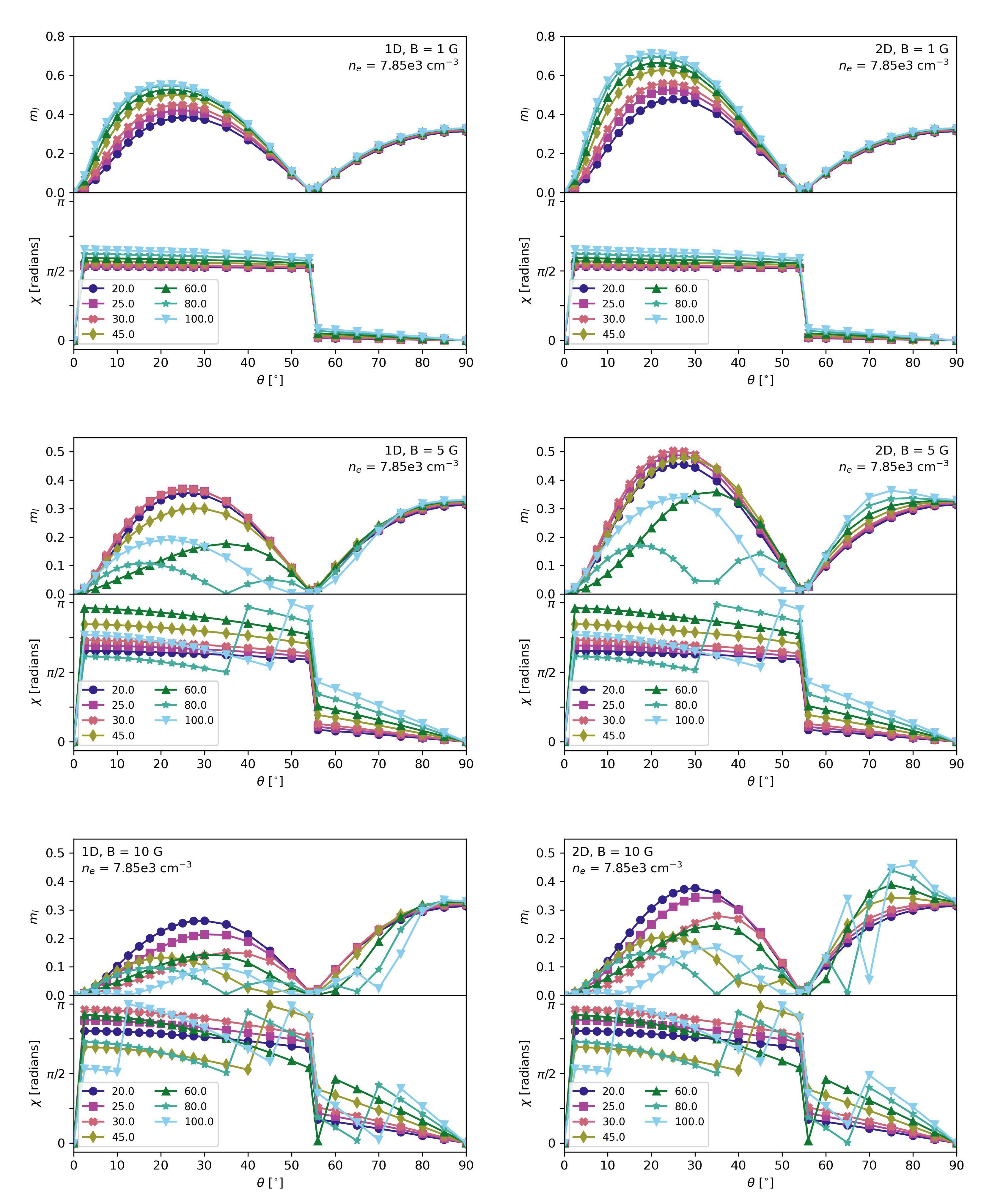
While behavior of the total intensity, , and fractional circular polarization, , do not change significantly compared to the solutions with no Faraday Rotation, the effects of Faraday Rotation on linear polarization can be seen for cm-3 at the highest sampled optical depths (Figure 8). For the weaker Faraday Rotation seen with 1 G magnetic fields, this manifests itself as a slight decrease in the amplitude of the fractional linear polarization and a slight rotation in EVPA as a function of , though the EVPA flip and the general profile is preserved. However, further increasing the magnitude of the Faraday Rotation can instigate additional EVPA flips. For a 5 G magnetic field, a secondary flip only occurs for optical depths ; however, with 10 G magnetic fields, we see as many as three additional EVPA flips occurring by an optical depth of 100, with the first appearing at an optical depth of 45. The increasing number of minima in that accompanies the appearance of new EVPA flips, also has the effect of further decreasing the maximum that can be present at line center.
Even for a given electron density and magnetic field strength, the Faraday Rotation term . As expected, no change in linear polarization is present for magnetic fields perpendicular to the line of sight (), with the effect of Faraday Rotation generally more apparent as decreases. We also reproduce the expected non-reciprocity of Faraday Rotation; for bi-directional clouds, the Stokes solution is symmetric about cloud center.
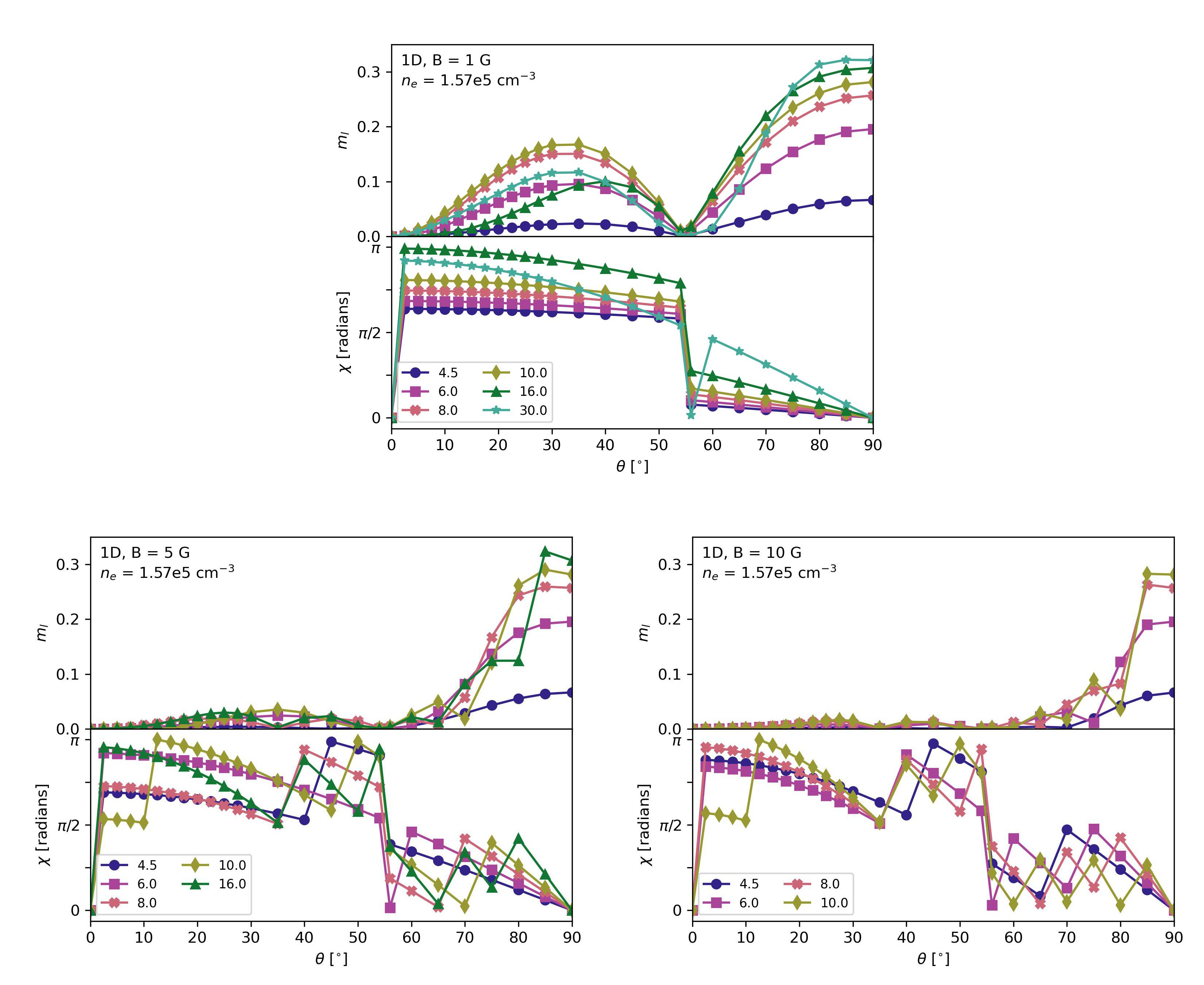
The linear polarization for cases with a higher electron density of cm-3 is shown in Figure 9 up to the maximum total optical depth achieved for each sampled magnetic field strength. With a 1 G magnetic field (), the appearance of secondary EVPA flips begins for . The fractional linear polarization at lower , while still showing a smooth variation with , is suppressed enough that it never exceeds the fractional linear polarization at once the Van Vleck angle has reached its characteristic value.
Further increasing the Faraday Rotation to ( 5 G) or 3.86 ( 10 G) not only further suppresses linear polarization at low , keeping it below (5 G) or (10 G), but also gives rise to deviations from the previously smooth profile. The latter hints that structure below the resolution of sampled has arisen, particularly at larger . With a 5 G magnetic field, the secondary EVPA flips occur for as low as 4.5. However, for a 10 G magnetic field, the Faraday Rotation generated EVPA flip occurs for an optical depth as low as 1.7, preceding the appearance of the Van Vleck angle. Unlike the Van Vleck angle, which appears first for high before approaching its characteristic value, the Faraday Rotation generated flip occurs first at low , and migrates to higher with increasing .
The failure of full solutions with cm-3 to converge for higher optical depths to the desired precision may be improved by increasing the resolution of the line of sight optical depth, , though this would also cause a corresponding increase in compuation time. For the maximum Faraday Rotation case analyzed here, there are a total of six EVPA flips along the line of sight at with an optical depth of 10. This leaves an average of only bins between successive EVPA flips along a single ray’s path, which may result in degraded accuracy in the line of sight integration and the resulting full inversion solution.
6 Tests against previous work
We consider here a number of comparisons between results of the current work and those of earlier authors, from the analytical results of GKK to the recent analysis by Lankhaar & Vlemmings (2019), hereafter LV19.
6.1 Comparison with GKK and Watson et al. models
The original benchmark for our code, PRISM, is that it should be able to reproduce the results for both linear and circular polarization in Watson & Wyld (2001), even though the methods of analysis are not quite the same, and the numerical implementation is different. We additionally compare our results with the predictions of GKK, but we do not expect our code to achieve the GKK limits.
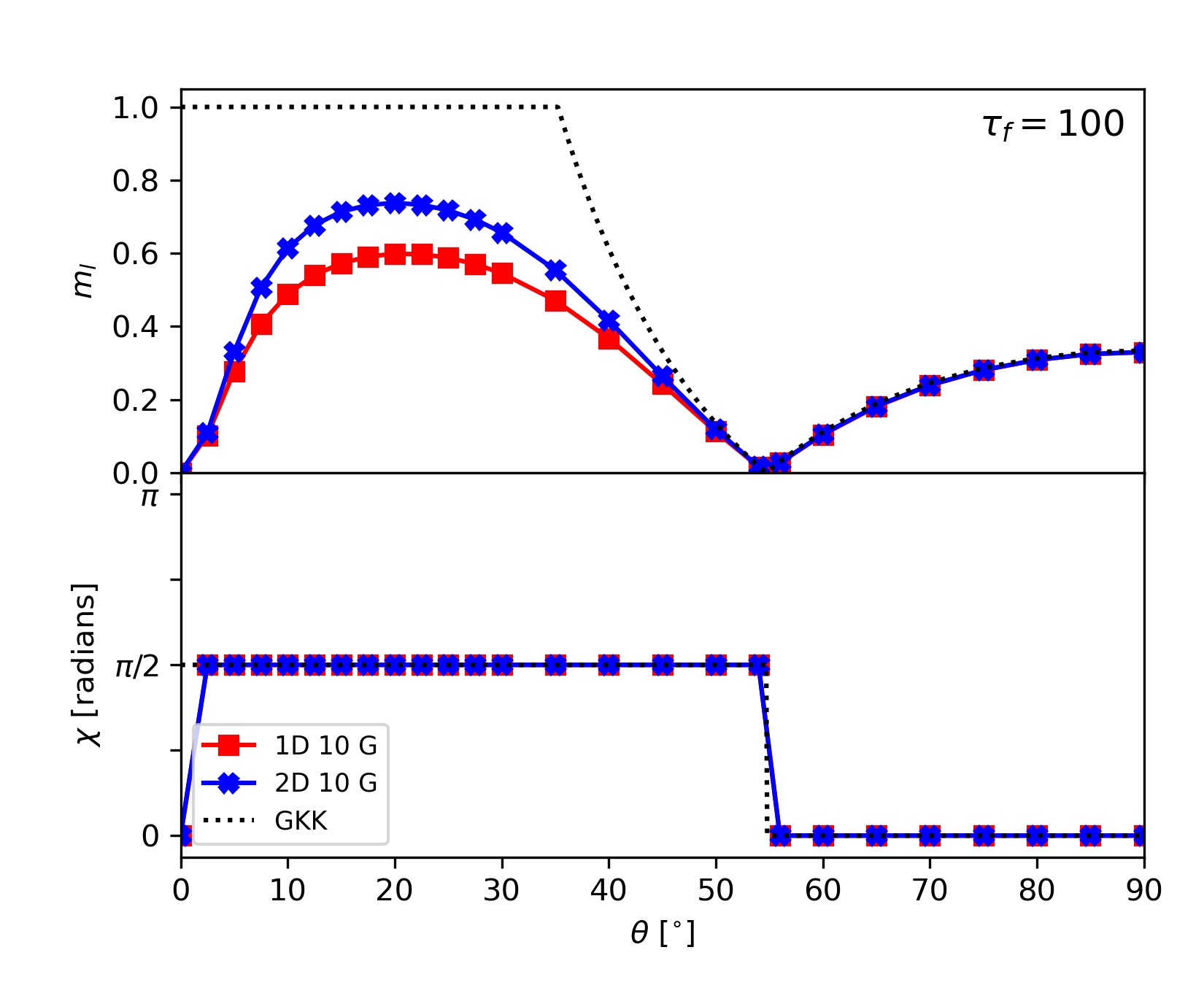
As a demonstration, we show in Figure 10 the linear polarization fractions of two of our models, compared with the GKK prediction (in the appropriate limit of Doppler width Zeeman splitting stimulated emission rate, essentially GKK case 2a) as a function of the angle between the directions of propagation and the magnetic field. We note that the maser depth used () implies a level of saturation that exceeds the capacity of our model, but we use this high value to demonstrate the very slow convergence towards the GKK limit of 100% linear polarization for angles significantly less than the Van Vleck value (see also Figure 3). At angles greater than this value, the predictions of GKK and our model agree almost perfectly.
We do note that, as seen in Figure 10, the fractional linear polarization at lower is higher when integrating along two bi-directional rays than with the single ray model. In the case of a fully 3-dimensional model, saturation is enforced through an angle-dependent function analogous to a solid-angle averaged intensity. Early results222http://www.jb.man.ac.uk/ setoka/SEtoka_EWASS2019_ePoster.pdf are not complete enough to show whether the trend of increasing with the number of rays continues at values of smaller than the Van Vleck angle.
| (1D) | (2D) | |
|---|---|---|
| 3.5 | 3.5 | |
| 4.3 | 4.4 | |
| 6.1 | 7.4 | |
| 9.0 | 13 | |
| 19 | 32 | |
We have computed unidirectional and bidirectional solutions to compare directly against the linear and circular polarization fractions presented in Watson & Wyld (2001). The saturation intensity used for normalization in that work, , and the saturation intensity defined here, , are equivalent, though the former is a specific intensity per frequency, while the latter is in specific intensity per angular frequency. Therefore, the dimensionless Stokes parameters presented here are directly comparable to the dimensionless Stokes parameters in Watson & Wyld (2001). The unpolarized seed radiation used in the calculations presented here, , is between the two values of and used as seed radiation in that work. In addition, they use the unitless Stokes I as a proxy for maser saturation. Table 2 outlines the conversion between unitless Stokes and the total optical depth required to reach that Stokes at line center for uni- and bi-directional integration.
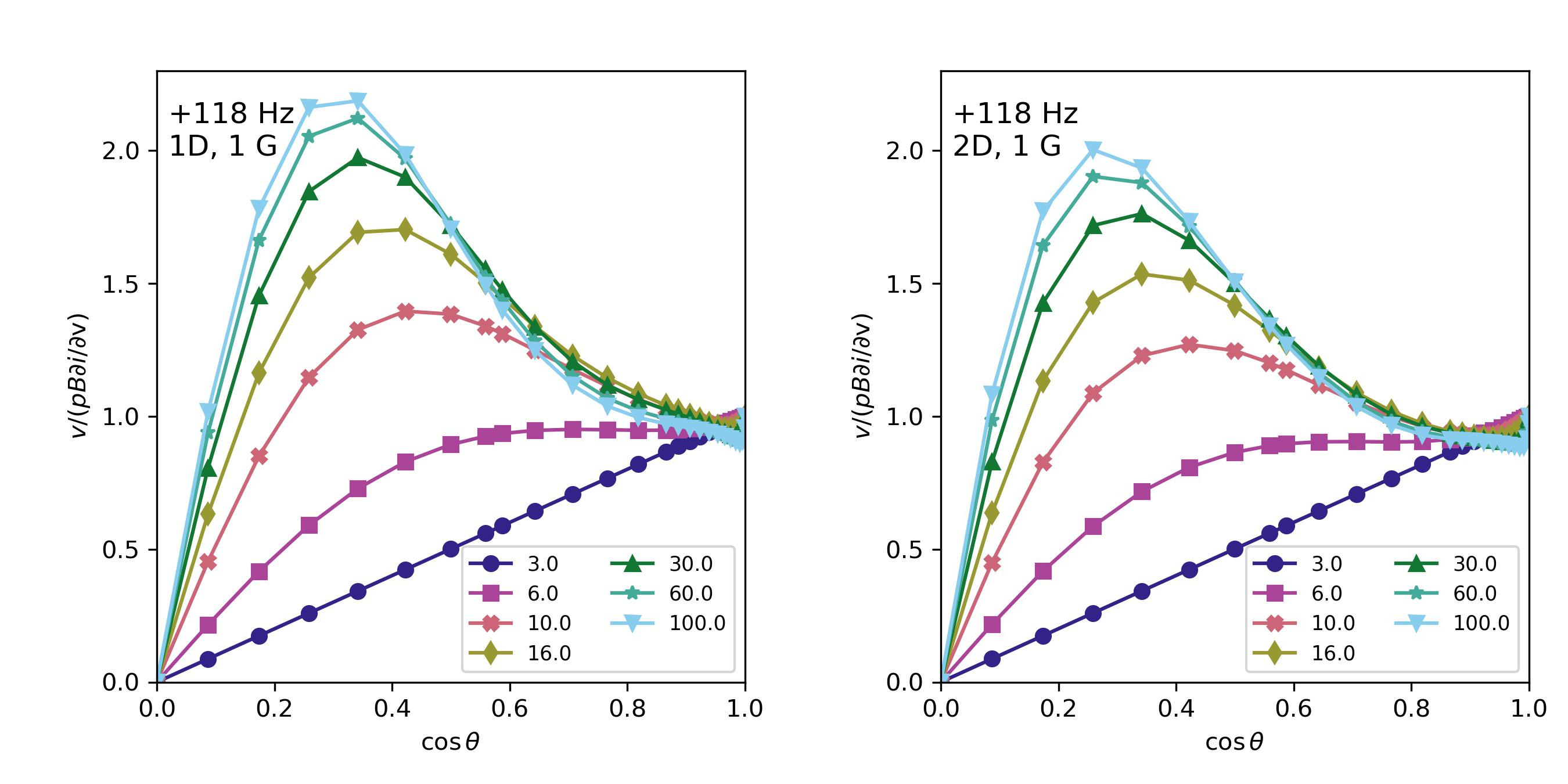
For comparison with Figure 1 of Watson & Wyld (2001), the unitless Stokes normalized by the partial derivative of the unitless Stokes with respect to velocity and the Zeeman splitting in velocity space, , is plotted in Figure 11 for uni- and bi-directional masers. While the figures plotted are for 1 G magnetic fields, the normalization by the Zeeman splitting in velocity space removes any variation with . Data plotted is calculated at a single bin offset ( Hz) from line center, the normalization by the partial derivative removes any significant variation with frequency out to bins ( kHz).
As seen in Figure 11, the framework presented here reproduces the dependence of circular polarization on from Watson & Wyld (2001). At low , as expected for their equivalent saturation of , with the dependence becoming peaked as optical depth or saturation increases. While the seed radiation used here is intermediate to the two values used in Watson & Wyld (2001), they note that the magnitude of the seed radiation only affects this dependence for , at which point the peaks with the larger seed radiation of become smaller than for the smaller seed radiation of . The intermediate equivalent seed radiation used in the solutions presented here yields a peak for a uni-directional integration with and for a bi-directional integration with , both of which are within the range of peak values produced by the larger and smaller seed radiation from Watson & Wyld (2001) for .
6.2 Comparison with Lankhaar and Vlemmings, 2019
| 1D Min | 1D Max | 2D Min | 2D Max | 1D Min | 1D Max | 2D Min | 2D Max | |
|---|---|---|---|---|---|---|---|---|
| 1 G | -5.5 | 4.1 | -5.2 | 3.8 | -9.1 | 0.8 | -8.9 | 0.5 |
| 2 G | -5.8 | 3.8 | - | - | -9.4 | 0.5 | - | - |
| 5 G | -6.2 | 3.4 | -5.9 | 3.1 | -9.8 | 0.1 | -9.6 | -0.2 |
| 10 G | -6.5 | 3.1 | -6.2 | 2.7 | -10.1 | -0.2 | -9.9 | -0.5 |
In a work that draws heavily on earlier models in the Watson et al. series (see above), LV19 have developed the very able code champ for the analysis of a wide range of molecules and transition types. As such, it goes, in some respects, considerably beyond the scope of the present work. However, there are significant differences in the theoretical construction and numerical implementation that should be discussed, and a successful agreement in the principal results then strongly suggests that the underlying theory is correct, independently of the exact methods used.
Apart from the obvious improvements in LV19 relating to more general Zeeman patterns and hyperfine structure, and our inclusion of a counter-propagating ray and Faraday rotation, the main differences between the LV19 analysis and that in the current work can be summarised as:
-
1.
In LV19, the time-dependence of off-diagonal elements of the DM is integrated out, and a subsequent steady-state approximation applied to the level populations to reduce the system to an algebraic (matrix) equation. In the present work, we follow rather the method of Dinh-v-Trung (2009a) in Fourier-transforming the equations to the frequency domain, eliminating the time-dependence of all DM elements in the process (see work leading to our equations 7 - 10) for a finite sampling time of the order of the reciprocal channel width.
-
2.
The populations are recovered from a matrix inversion procedure in LV19; in the present work we make a formal solution of the coupled radiative transfer equations in order to algebraically eliminate the Stokes parameters, leaving a set of coupled algebraic equations in the inversions, our eq.(27) and eq.(28). The numerical solutions in the two works therefore rely on different sets of algorithms.
-
3.
The classical saturation approximation (described at the beginning of Appendix A) is probably equivalent to the ‘sharply-peaked’ approximation to the homogeneous lineshape function mentioned in LV19, and used in Watson & Wyld (2001). If this is so, the results presented in LV19 use a more general approximation, based on a Taylor expansion of the lorentzian profile, and champ can therefore be used at higher (but not arbitrary) levels of saturation than the present work.
-
4.
Parameters used by the codes differ somewhat. LV19 scales maser saturation directly, using the base-10 logarithm of the ratio of the stimulated emission and Zeeman rates, rather than indirect adjustment as a result of the changing optical depth, . We discuss below some problems related to the definition of the stimulated emission rate.
-
5.
The formalism presented here sets the type 2 off-diagonal elements of the DM to zero, unlike the results presented in LV19 from their method iii. See Section 7.3 for a discussion of the affect of this approximation.
Before introducing a formal definition of the stimulated emission rate, we note that historically it has been based on equations like eq.(44) of Nedoluha & Watson (1990) in which the Stokes parameters are dimensionally specific intensities, and outside this subsection we also refer to stimulated emission rates in this sense. In eq.(44) of Nedoluha & Watson (1990), their is consistent with the stimulated emission rate as an Einstein B-coefficient multiplied by a line-center specific intensity (and trigonometric functions via the various dipole products). This interpretation is backed by the expression for the low-intensity boundary condition on Stokes I near the beginning of Section III of Nedoluha & Watson (1990). We now define the stimulated emission rates used in the present work.
The stimulated emission rate per substate transition in each angular frequency bin, , can be calculated for the solution presented here from the unitless Stokes solution at the end of the cloud:
| (37) |
| (38) |
noting that our , and specifically the line-center , are consistent with the traditional stimulated emission rate from Nedoluha & Watson (1990) since the dimensionless Stokes parameters are scaled to the specific intensity, from eq.(29). However, as we have full spectral information, we choose to write the stimulated emission rate calculated at line center as
| (39) |
and define a separate, total stimulated emission rate that encompasses the full spectral emission:
| (40) |
The stimulated emission rate in the bin, may be viewed alternately as the rate, in s-1, per angular frequency integrated over the width of the angular frequency bin: . Then, summing the mean stimulated emission rate over the angular frequency bins gives a measure of the total stimulated emission rate represented by the full spectral linewidth.
We continue using for consistency, though it is worth noting that the dimensionless solutions presented here with no Faraday Rotation are independent of . The total Zeeman width is calculated as . Calculating for each solution, we find that varies as a function of alone, and may therefore be viewed as a proxy for within a given parameter set. The ranges of values calculated across all for a given magnetic field strength and number of rays are shown in Table 3, as well as the values calculated at line center, . In general, decreases with increasing magnetic field strength and is slightly lower for a bi-directional integration than for a uni-directional integration, but shows no significant variation with the inclusion of nonzero Faraday rotation.
The ranges of values calculated at line center, , follow the same trend, with typical values below , though it is not a direct, uniform scaling. We discuss the relation between and further in Section 7.4. For the purposes of this comparison with LV19, we will use the line center value, , as they do, for a more direct comparison. However, we note that, while the non-linearities in the relation between and do cause minor adjustments in the precise form of the results presented as a function of and here, the general trends are unchanged.
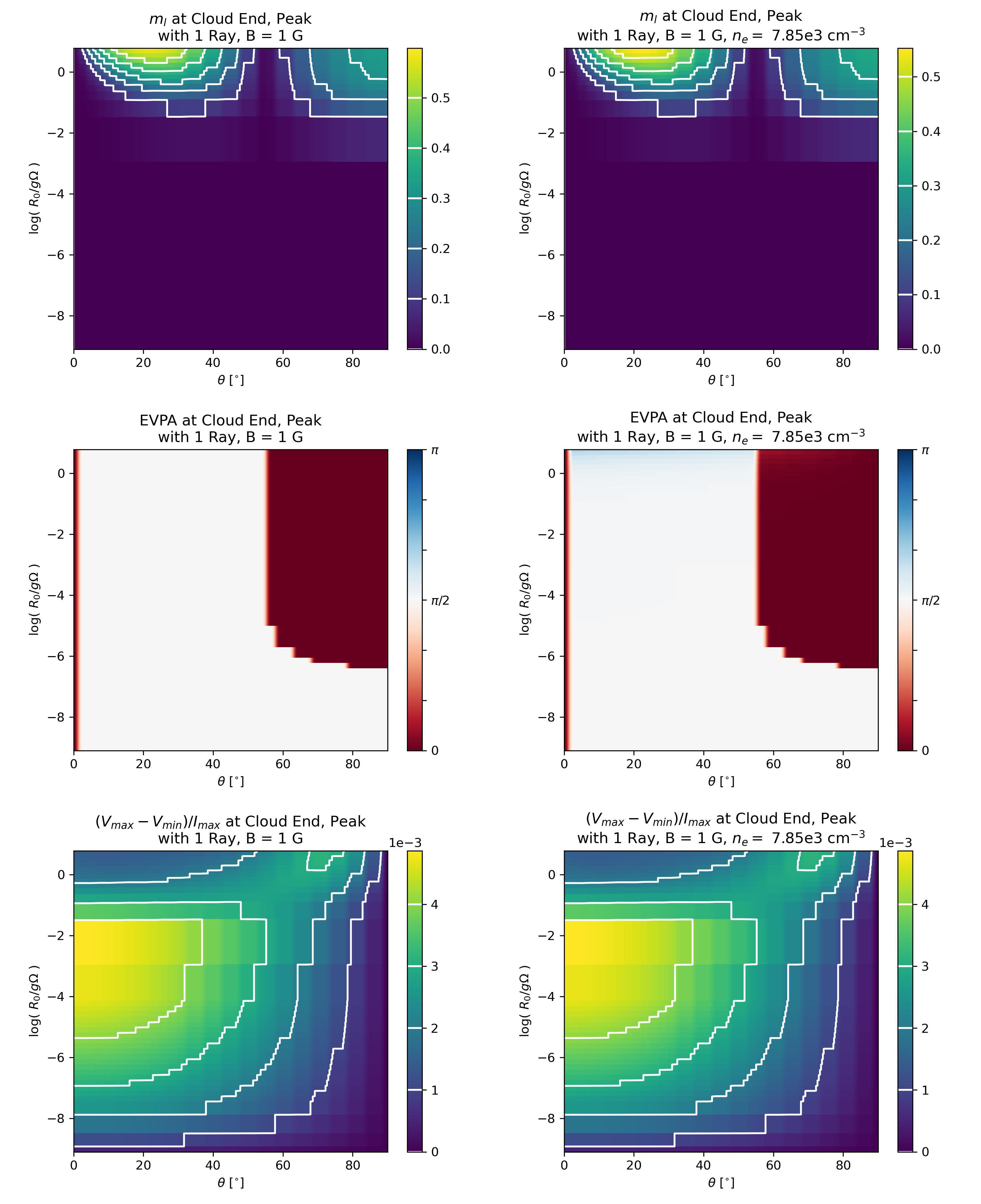
Figure 12 shows the line center and EVPA for the 1-directional, 1 G solutions with no Faraday rotation and Faraday rotation with , as well as their respective ranges in Stokes across normalized by line center stokes (referred to as in LV19) for comparison.
While the ranges of covered by our solutions differ from those of LV19, the most notable difference in linear polarization between the solutions presented here and those of LV19 in the overlapping region (-3 to 0.8) regards the onset and/or disappearance of the EVPA flip with increasing maser saturation. The 1 G SiO solutions of LV19 have a EVPA rotation at the Van Vleck angle only occurring for low -2 to -3, which smooths out and disappears with increasing . Conversely, the solutions presented in this work show no smoothing or disappearance of the EVPA flip with increasing saturation between up to our maximum 0.8. At lower saturation than that covered by LV19, our solutions also show the instantaneous EVPA flip appearing for large and approaching the Van Vleck angle as increases.
The difference in the appearance and behavior of the EVPA rotation also causes a marked difference in the profile, with the minimum at the Van Vleck angle persisting in our solutions to the largest computed values of , once it has set in. The LV19 solutions also show a distinct peak and subsequent decrease in for increasing , with the peak occurring at as in the 1 G SiO solution.
While the solutions presented here only go up to , we see no indication of a decrease in with increasing saturation above in our solutions with no, or weak, Faraday rotation. However, this behavior is visible in our solutions with stronger Faraday rotation, but it occurs at lower values of (eg. Figure 13). Although not present in the calculated solutions for with a low , does begin decreasing at the highest levels of achieved here, as the Faraday rotation begins suppressing linear polarization. The suppression of at high increases significantly for particularly for the peak at lower . Notably, the solutions from LV19 method (iii) do allow for Stokes QU conversion by allowing for non-zero , much like our inclusion of non-zero Faraday rotation with . Therefore, the comparison between the solutions derived here and those of LV19 may be most appropriately applied to our solutions with nonzero Faraday rotation.
In addition to terms linking Stokes to and , the condition also introduces terms into the maser propagation equations that couple and to . These all arise from a shift of the ‘good’ symmetry axis for quantization away from and towards the propagation axis as increases. If the magnetic field is still used as the quantization axis when then these compensatory terms enter through the type 2 off-diagonal elements of the DM, and such terms are included in LV19 and in Nedoluha & Watson (1994). However, we also note that, while the line center values only extend up to to in the solutions presented here, the stimulated emission calculated using the full line breadth, , are to times the order of magnitude of .
The circular polarization metric used by LV19, , is likewise shown in Figure 12. The isotropic LV19 solutions for SiO in a 1 G field have reaching a peak of around at . Starting at saturation , their has reached for to . In our solutions, with and without Faraday rotation, shows a marked peak and decrease at low with increasing , with the peak occurring around to for our 1 G solution. However, our solutions have no decrease in for small as . Our solutions also show a secondary, lower amplitude peak in , peaking for at the highest .
Notably, the values of presented here for a 1 G magnetic field are below the levels of the contours in LV19. Despite measuring the full peak-to-valley range of Stokes v, ’s normalization by the line center rather than the value of Stokes at the same frequency at which Stokes is also being measured results in being significantly lower than the presented previously in this paper. However, our 1 G solutions still lack the higher values of LV19 for for most . In addition, our B10 G solutions show the same behavior in as the 1 G solutions presented in Figure 12 with values extending up to . While the saturation regime for those only extends up to , the secondary peak in our solutions that starts forming at high mentioned above, remains limited to high values of , and, at , still falls shy of reaching the level of the LV19 contours for the same magnetic field.
As discussed below in section 7.3, the assumption by the present work that type 2 off-diagonal DM elements are negligible compared to those that represent the electric dipole-allowed transitions may explain some of these discrepancies at the higher values of .
7 Discussion
We have demonstrated that our maser polarization code PRISM behaves as expected as the Zeeman splitting is varied from very small values, of order similar to the width of the homogeneous response profile of the molecules, to values that substantially exceed the inhomogeneous (Doppler) width. In the latter case, the solutions correspond to the circularly-polarized Zeeman doublet when the field and propagation directions are parallel, and to a linearly-polarized triplet when these directions are perpendicular. We have compared results with the earlier work of GKK (finding agreement in the expected range of angles), with the work of Watson’s group, where we have demonstrated agreement for uni- and bi-directional masers at stimulated emission rates up to approximately , where implies at line center, and finally with the recent predictions of the champ code, noting that we have restricted our analysis to lower levels of saturation than those in Lankhaar & Vlemmings (2019). Overall, we consider the degree of agreement between the various models to be very good, considering the differences in the analysis strategies and numerical algorithms. We consider specific areas of further discussion below.
7.1 Consequences of approximations
The main approximations that limit the degree of saturation accessible to our code are those that form part of the ‘classical saturation’ set (see Appendix A). We have limited our examples to modest levels of saturation on account of these simplifications. The first of these, no correlation between different Fourier components of the radiation field, is not problematic unless the input radiation to the maser is itself coherent. However, the second approximation must be lifted as a prerequisite for a fully semi-classical response. This requires working with the unsimplified eq.(9) and eq.(10) as the descriptions of the inversions, noting that, in this pair of equations, the maser field is represented by electric field amplitudes. An expression in terms of the Stokes parameters is only possible if the third assumption (gaussian statistics) is maintained, but departures from gaussian behaviour are to be expected, starting at line centre, and moving towards the wings at larger signal strengths (Dinh-v-Trung, 2009b, a). Replacement of the Dirac -function approximation with full lorentzian homogeneous lineshape functions is therefore of limited value in increasing accessible levels of saturation without making more significant changes to the code to incorporate fully semi-classical saturation. Equations (9) and (10) are not completely intractable. One approach, that follows the style of solution in the present work, is to make a formal solution of the frequency-domain electric field complex amplitudes, eliminating these from eq.(7)-eq.(10) in favor of off-diagonal DM elements. Then, eq.(9) and eq.(10) are used to eliminate the inversions from eq.(7) and eq.(8), leaving a set of non-linear algebraic equations in the off-diagonal DM elements. Another possibility is to use the method derived in Wyenberg et al. (2021), which is a generalisation of the Fourier-based method developed by Menegozzi & Lamb (1978).
7.2 Accessible range of saturation
The limit placed on the degree of saturation in (Watson & Wyld, 2001) is that the stimulated emission rate must be considerably less than the Zeeman splitting (). This limit is mentioned in the text following their eq.(12), and is applied because they use classical rate equations rather than a semi-classical (DM) representation of the molecular response. For our models with s-1 and magnetic fields of 1-10 G, we have in the approximate respective range 1/3-1/30 at an optical depth of . Our use of an upper limit optical depth of 30 therefore conforms to the for the larger magnetic fields, but is becoming marginal for 1 G. At an optical depth of 100, the approximation fails, even for the highest field used.
Nedoluha & Watson (1990) extend the range of accessible saturation by adopting a semi-classical molecular response. As the present work also uses a DM, we discuss here whether we may also extend our saturation limit beyond the constraint. There are two possible reasons why we should not do this: the first is the presence of off-diagonal DM elements within a single -state of the molecule. However, (Nedoluha & Watson, 1990) also ignore these, so we defer discussion of them to Section 7.3 below. The remaining reason that might limit our degree of saturation is the use of classical reductions (see Section 7.1), particularly the replacement of lorentzian homogeneous profiles by -functions. For a brief understanding of the consequences of this, we would always want to resolve the Zeeman splitting, resulting in maximum channel widths of order in frequency. Lorentzian profiles power broaden according to , which, for strong saturation, may be inverted to yield , where is the original width parameter. Setting , and , we then find we require , exactly the criterion adopted for the upper limit of magnetically induced polarization in GKK. We also note that Nedoluha & Watson (1990) continue to use the magnetic field as a quantization axis in this regime, without moving to the ray-based quantization of the GKK Case 3, where . Adopting the limit might allow us to access saturation levels as high as perhaps 10% of , or 9000 for a 1 G field. However, a more accurate analysis suggests greater caution is required.
A power-broadened homogeneous lineshape is described, for example, in Vitanov et al. (2001), and a unity-normalized version in offset frequency looks like,
| (41) |
where for mean intensity and saturation intensity , and , as before, is the unsaturated homogeneous width. Suppose that we wish to limit semi-classical effects to population pulsations with magnitudes smaller than 10% of the total inversion: we can obtain the corresponding half-width of the power-broadened function by integrating from eq.(41) over the limits zero to the desired half width, , and equating the result to 0.95. The result of the integration is
| (42) |
The width is rather large, owing to the relatively broad wings of the lorentzian function compared to a gaussian. We now set this width equal to the actual Fourier channel widths used. For the SiO parameters applied to the models in Figure 3, the channel width is s-1, so using the value of 5 s-1 for introduced above, we arrive at . This figure is not much less restrictive than that imposed by , but probably means that , the largest degree of saturation used in this work is acceptable, but higher values should be modeled only if the simplifications described in Section 7.1 are lifted. Our value of derived above is also consistent with the figure of 100 stated in Section 5.1.1 of LV19.
7.3 Off-Diagonal DM elements
Off-diagonal elements of the DM may be divided into two types: those (type 2) that represent the coherence between levels that would be degenerate in the absence of an applied magnetic field, and the remainder (type 1) between levels that would not. The center frequency of a type 2 transition is therefore comparable to the spread of a single Zeeman group, or a few Doppler widths at most, whilst the center frequency of a type 1 transition is comparable to the rest frequency of the unsplit transition, in the present work. Transitions of the two types behave differently when the rotating wave approximation is applied. The off-diagonal DM element of a type 2 transition satisfies a differential equation in the time domain that has no direct coupling to an inversion: it can develop only from itself and from other off-diagonal DM elements. In the system considered in the present work, there are three possible type 2 DM elements, each of which is coupled directly to a pair of off-diagonal DM elements representing electric dipole-allowed transitions.
We note that in the present work the type 2 off-diagonal elements are set to zero. However, Lankhaar & Vlemmings (2019) do not make this assumption, and include the type 2 elements, as do Nedoluha & Watson (1990), where they are assumed to be constant when solving for the DM elements (their eq.(10)). We can estimate the consequences of ignoring the type 2 DM elements by including the correction due to these terms in a Fourier component of a type 1 element. With these corrections, a reduced version of eq.(7) for with , , and considering one hand of polarization only, takes the form
| (43) |
where complex lorentzian functions corresponding to type 2 transitions have their quantum-number pairs shown in square brackets in the superscript. Equation 43 demonstrates that the terms within the sums over that result from the inclusion of type 2 off-diagonal DM elements are of order with respect to 1, and therefore are likely to become significant under strongly saturating conditions. Further, the type 2 contributions are modified by the product of pairs of complex lorentzian functions so their effect will increase as these functions power-broaden. The effect of the type 2 terms is deleterious to the coherence of the transition, both reducing the coupling to its own inversion (top line in eq.(43)), and by introducing population mixing via terms involving inversions in the other two type 1 (dipole-allowed) transitions (lower line in eq.(43)). Overall then, the type 2 off diagonal elements will reduce the polarization at very high degrees of saturation, even if they are initially set to zero, and are an additional reason why our current model will become unreliable for stimulated emission rates significantly higher than .
7.4 The significance of nonzero Stokes V
Many previous publications related to maser polarization for small Zeeman splitting (much smaller than the Doppler width) ignore circular polarization entirely, either for simplicity, or citing the antisymmetric profile of Stokes V. GKK do discuss off-resonance propagation, but their strong result in Case 2 is of zero circular polarization at line-center. Another major work that considers only line-center amplification is Deguchi & Watson (1990), and this results in linear polarization only. The formalism presented here includes the propagation of Stokes , as well as the retention of the full Stokes profile as a function of angular frequency, . This allows a comparison of not only the relative intensities of the linearly- and circularly-polarized emission, but also a comparison of the maximum values of and achieved, as the anti-symmetric profile of Stokes necessitates that its peak occurs away from the peak in Stokes at line center.
To provide a sense of the relative amplitudes of and for the derived solutions, we plot as a function of and total optical depth, , for the uni-directional solutions for three magnetic field strengths, with and without Faraday rotation (Figure 14). At high , is still larger than around and the Van Vleck Angle, where . For solutions with stronger Faraday rotation, surpasses for large as the Faraday rotation suppresses .
Notably, in all cases with , the maximum is larger than the peak for . This trend does not appear to be driven by an amplification of from the decreased Stokes away from line center; a similar characteristic behavior is seen when comparing the peak and maximum . This behavior implies that, particularly at low saturation (), circular polarization is not negligible compared to linear polarization.
Another benefit of accounting for Stokes away from the line center is that it provides insight into the relation between the stimulated emission rate calculated at line center, , and the stimulated emission rate summed over the full line profile, . As shown in Figure 15, the relation between and as a function of is significantly non-linear across the range of solutions presented here, increasing by a factor of from to .
While this would have relatively little effect on the functional form of the results plotted in, say, Figure 12 and 13 if they were plotted using instead of (simply distorting some of the vertical scaling), it does suggest that caution may be warranted when using a stimulated emission rate calculated at line center, to infer the strength of the full stimulated emission rate, , even if includes nonzero Stokes at bins from the line center.
As can be seen in eq.37, Stokes is included in the calculation in the form of , despite the value of Stokes at line center being zero. Then, the ability for to accurately reflect the full is limited by the ability of Stokes to trace the peak strength of Stokes . However, the profile of Stokes can vary not only in amplitude, but also in the offset frequency from line center at which it peaks. Figure 15 also shows how the frequency at which Stokes peaks and the ratio between Stokes varies with . As increases from 0.1 to , the Stokes profile becomes narrower, and the fraction of the peak that occurs in the bin from line center increases. The Stokes term in contains a larger fraction of the total Stokes , and, as a result, increases with respect to . Then, as continues increasing beyond , the reverse occurs; the Stokes profile broadens, with the peak moving further from line center. Less circularly polarized flux is present in the bin from line center, and once again decreases.
8 Conclusion
We have derived expressions for velocity subgroup populations in a one-dimensional maser saturated by either 1 or 2 beams of polarized radiation, described by the Stokes parameters. This theory has been coded in a new computer program, PRISM. Using this program, we have demonstrated the expected amplification of circularly polarized Zeeman doublets and linearly polarized triplets in the large splitting case (), and that our code can show a smooth transition from this case to that of small splitting. In the small-splitting case, we show the appearance of the Van Vleck angle at low amplification, the independence of the linear polarization fraction from the magnetic field strength, under moderate to strong saturation, and the generation of circular polarization at off-center frequencies. PRISM can consider non-zero Faraday rotation, and we demonstrate the rotation of the EVPA and suppression of linear polarization with increasing magnetic field at a fixed free electron number density. We compare our PRISM results to the analytic predictions of GKK, to the numerical calculations from Watson & Wyld (2001), and to the more recent work of LV19. We find our results to be compatible with these other works, given the differences of approach and levels of approximation. We discuss the limitations of our model and code with regards to saturation, and we also discuss the development with saturation of overall levels of circular and linear polarization.
Appendix A Some Derivation Details
We make a classical reduction of eq.(7) - eq.(10) that has the following consequences: (1) Different Fourier components of the radiation field are uncorrelated at any degree of maser saturation; (2) There are no pulsations of the inversion, so it is restricted to the central Fourier component with ; (3) The statistics of the radiation are gaussian, and (4) Real lorentzians behave as Dirac -functions. Point (2) above dictates that in eq.(7) and eq.(8), reducing the sums to single terms. The sums survive in eq.(9) and eq.(10), but , allowing many terms to be combined. In particular, all off-diagonal DM elements now appear at Fourier component , allowing pairs of complex conjugate terms to be expressed as real parts. The off-diagonal elements are then eliminated from eq.(9) and eq.(10) using various versions of eq.(7) and eq.(8) with the sums collapsed as described above. The resulting equations contain pairs of complex field amplitudes that can be grouped and eliminated in favour of the Stokes parameters. The resulting equations,
| (A1) |
and
| (A2) |
express the saturation of velocity-subgroup inversions by the Stokes parameters of a ray in a single sample of duration equal to the reciprocal of the width of the Fourier channels. Our Stokes parameters have the definitions
| (A3) | ||||
| (A4) | ||||
| (A5) | ||||
| (A6) |
In equations A1 and A2, the only complex quantities that remain inside the large braces are the lorentzian functions that have the general definition
| (A7) |
where the superscript represent optional transitions for selection. The Zeeman shifts for the three transitions are for the transitions where is the absolute Zeeman shift. The transition has . It is straightforward to show that the real part of eq.(A7) is equal to half the real lorentzian,
| (A8) |
so that the real part operation () on the contents of the braces in eq.(A1) and eq.(A2) may be carried out by replacing all complex lorentzians with their real counterparts, and changing the 8 to 16 in the denominator multiplying the sums over .
The analysis proceeds by noting that the classical reduction allows eq.(A8) to be used as a representation of the Dirac -function, and this can be used to collapse the -sums in eq.(A1) and eq.(A2). The -function selects the transition, and velocity, dependent Fourier component centered on the local frequency . We use the shorthand expression , and similarly for the rest of the Stokes vector, to represent these frequencies as indices on the Stokes parameters. The somewhat reduced forms of eq.(A1) and eq.(A2) are
| (A9) |
and
| (A10) |
The in eq.(A9) and eq.(A10) are inversions in the velocity subgroup at velocity . It is advantageous to convert these into inversions, or molecular responses, at a particular frequency. To this end, we multiply eq.(A9) and eq.(A10) by the lorentzian-style function,
| (A11) |
and integrate over all velocities. The result is to select a particular velocity corresponding to the Zeeman-shifted frequency of the transition. If we define the response as
| (A12) |
and note that the Zeeman shifts for each transition type are for the transitions, where is a positive definite frequency shift, and for the transition, then we can re-cast eq.(A9) and eq.(A10) respectively as
| (A13) |
and
| (A14) |
A formal realization average over the Stokes parameters, which can be isolated statistically from the responses because of the assumption of gaussian statistics, replaces the single realization versions with the averaged forms , and similarly for the other Stokes parameters. Adoption of the shorthand notation , replacing the Zeeman shift of by frequency bins returns the analysis to eq.(11) and eq.(12) of the main text.
Appendix B Counter–Propagating Rays
The solution presented in Section 3 applies to a ray traveling in a given direction through the cloud, or Ray 1, in which the molecular populations have line of sight velocities denoted by , corresponding to the angular frequency with respect to line center, . To apply this solution to a pair of counter–propagating rays, we must first consider how the solution changes for Ray 2, traveling in the opposite direction through the same population. Comparing Ray 2 to Ray 1, we must make the following adjustments:
-
1.
The angle of the magnetic field to the line of sight, , is defined for Ray 1 as viewed from the end of the cloud that Ray 1 exits from. As preserves the directionality of the magnetic field, the corresponding angle between the magnetic field and line of sight for Ray 2 will be . Notably, the solution presented above only relies on in the form of , , and , so this point will only affect terms of un-squared , as .
-
2.
The orientation of Stokes and as defined for Ray 1 correspond to the orientation of Stokes and , respectively, for Ray 2. Stokes and are unchanged.
-
3.
Likewise, the generalized sky-plane angle, , as defined for Ray 1 corresponds to the orientation of as defined for Ray 2. The solution above only depends on in the form of and . Therefore, this modification will only affect terms of as .
The Stokes parameters for each of the two rays are first calculated separately following Equation 26. For Ray 1, the dimensionless gain matrix terms are given as defined in Equations 32 - 36. Defining all parameters discussed above by their Ray 1 values, the first two dimensionless gain matrix terms for Ray 2, and , do not change from their values for Ray 1. The remaining terms become:
| (B1) | |||||
| (B2) | |||||
| (B3) |
In addition, when calculating the Stokes parameters for Ray 2, Equation 26 must be integrated in the opposite direction.
As the population at each can only have one batch of effective Stokes parameters, we define the effective Stokes as the sum of the Stokes parameters from the two different rays. This is because the intensity at a given point is determined by the buildup of light from each of the two directions. However, according to point 2 above, Stokes and have to be inverted to be combined with Stokes and :
| (B4) | |||||
| (B5) | |||||
| (B6) | |||||
| (B7) |
as defined in the reference frame of Ray 1. Of course, the Ray 2 Stokes parameters are integrated in tau starting from the opposite end of the maser as the Ray 1 Stokes parameters.
Since the unitless inversions represent the molecular energy state of the population, there must also be one unified value for each inversion at any point in the parameter space. These are the values that are being solved for within the system of equations. While the formulae that are used to calculate them (Equations 27 and 28) utilize the total effective stokes parameters from equations (B4) - (B7), they are still dependent on the angles and , which are different for each of the two rays.
However, a closer inspection of Equations 27 and 28 reveals that the only resulting terms that change signs between Rays 1 and 2, and , only appear when multiplied by Stokes and , respectively, which also change signs between reference frames. Therefore, the effective inversion as calculated from the effective Stokes parameters for both rays combined, , is the same regardless of the reference frame in which it was calculated.
Appendix C Loss of Van Vleck Angle at low intensity
The presence of a Van Vleck angle, at which is a minimum, between field angles of and is a feature of a wide range of conditions encompassing low to moderate saturation that are discussed in more detail in Section 5.2. The establishment of the angle for a constant magnitude magnetic field and increasing optical depth is shown graphically in Figure 3. We note that for very strong saturation, LV19 expect the Van Vleck angle to disappear again. We prove here that there is no Van Vleck angle in the limit of low intensity, in the sense that the gain coefficients in all the Zeeman transitions remain approximately constant.
In the case where there is no Faraday rotation, , and zero Stokes- at line centre, the following equations for propagation in the central frequency bin () can be derived from eq.(13) and the gain matrix in eq.(20) with components from eq.(21) and eq.(22):
| (C1) |
| (C2) |
where the subscript has been dropped for brevity. The gain coefficients in the equations above follow the pattern . The two propagation equations above can be added and subtracted to form equations in the sum and difference of the Stokes parameters. With the assumption that the gain coefficients are constant (very weak saturation) the sum and difference equations may be integrated to yield,
| (C3) |
where , and
| (C4) |
Subtraction of eq.(C4) from eq.(C3), and the assumption of an unpolarized background of intensity , leads to the following equation in only:
| (C5) |
Equation C5 may be differentiated with respect to , and the result equated to zero to investigate turning points. These are found only at angles satisfying , so there are no turning points in between and except at the end-points of the range. It is also straightforward to show that there are no zeros of in the same range by setting the left-hand side of eq.(C5) to zero and then taking the logarithm of the expression in square brackets. In this case a common factor of can be extracted, so there are also no zeros in the selected range of the angle.
References
- Assaf et al. (2013) Assaf, K. A., Diamond, P. J., Richards, A. M. S., & Gray, M. D. 2013, MNRAS, 431, 1077, doi: 10.1093/mnras/stt242
- Astropy Collaboration et al. (2013) Astropy Collaboration, Robitaille, T. P., Tollerud, E. J., et al. 2013, A&A, 558, A33, doi: 10.1051/0004-6361/201322068
- Astropy Collaboration et al. (2018) Astropy Collaboration, Price-Whelan, A. M., Sipőcz, B. M., et al. 2018, AJ, 156, 123, doi: 10.3847/1538-3881/aabc4f
- Boboltz & Diamond (2005) Boboltz, D. A., & Diamond, P. J. 2005, ApJ, 625, 978, doi: 10.1086/429656
- Caswell et al. (2021) Caswell, T. A., Droettboom, M., Lee, A., et al. 2021, matplotlib/matplotlib: REL: v3.4.3, v3.4.3, Zenodo, Zenodo, doi: 10.5281/zenodo.5194481
- Chandrasekhar (1950) Chandrasekhar, S. 1950, Radiative transfer.
- Deguchi & Watson (1986) Deguchi, S., & Watson, W. D. 1986, ApJ, 302, 750, doi: 10.1086/164036
- Deguchi & Watson (1990) —. 1990, ApJ, 354, 649, doi: 10.1086/168722
- Deguchi et al. (1986) Deguchi, S., Watson, W. D., & Western, L. R. 1986, ApJ, 302, 108, doi: 10.1086/163977
- Dinh-v-Trung (2009a) Dinh-v-Trung. 2009a, MNRAS, 399, 1495, doi: 10.1111/j.1365-2966.2009.15369.x
- Dinh-v-Trung (2009b) —. 2009b, MNRAS, 396, 2319, doi: 10.1111/j.1365-2966.2009.14901.x
- Elitzur (1992) Elitzur, M. 1992, Astronomical masers (Dordrecht: Kluwer)
- Elitzur & Asensio Ramos (2006) Elitzur, M., & Asensio Ramos, A. 2006, MNRAS, 365, 779, doi: 10.1111/j.1365-2966.2005.09770.x
- Garcia-Barreto et al. (1988) Garcia-Barreto, J. A., Burke, B. F., Reid, M. J., et al. 1988, ApJ, 326, 954, doi: 10.1086/166154
- Goldreich et al. (1973) Goldreich, P., Keeley, D. A., & Kwan, J. Y. 1973, ApJ, 179, 111, doi: 10.1086/151852
- Gray (2012) Gray, M. D. 2012, Maser Sources in Astrophysics (Cambridge, UK: Cambridge University Press)
- Gray et al. (2019) Gray, M. D., Baggott, J., Westlake, J., & Etoka, S. 2019, MNRAS, 486, 4216, doi: 10.1093/mnras/stz1137
- Gray et al. (2020) Gray, M. D., Etoka, S., Travis, A., & Pimpanuwat, B. 2020, MNRAS, 493, 2472, doi: 10.1093/mnras/staa424
- Gray et al. (2018) Gray, M. D., Mason, L., & Etoka, S. 2018, MNRAS, 477, 2628, doi: 10.1093/mnras/sty576
- Green et al. (2014) Green, J. A., Gray, M. D., Robishaw, T., Caswell, J. L., & McClure-Griffiths, N. M. 2014, MNRAS, 440, 2988, doi: 10.1093/mnras/stu429
- Gustafsson & Höfner (2004) Gustafsson, B., & Höfner, S. 2004, Atmospheres of AGB Stars, 149–245, doi: 10.1007/978-1-4757-3876-6_4
- Haëck (2021) Haëck, C. 2021, tol-colors, v1.2.1, GitHub. https://github.com/Descanonge/tol_colors
- Hamaker & Bregman (1996) Hamaker, J. P., & Bregman, J. D. 1996, A&AS, 117, 161
- Harris et al. (2020) Harris, C. R., Millman, K. J., van der Walt, S. J., et al. 2020, Nature, 585, 357, doi: 10.1038/s41586-020-2649-2
- Hunter (2007) Hunter, J. D. 2007, Computing in Science and Engineering, 9, 90, doi: 10.1109/MCSE.2007.55
- Ireland et al. (2011) Ireland, M. J., Scholz, M., & Wood, P. R. 2011, MNRAS, 418, 114, doi: 10.1111/j.1365-2966.2011.19469.x
- Kemball et al. (2011) Kemball, A. J., Diamond, P. J., Richter, L., Gonidakis, I., & Xue, R. 2011, ApJ, 743, 69, doi: 10.1088/0004-637X/743/1/69
- King & Florance (1964) King, J. I. F., & Florance, E. T. 1964, ApJ, 139, 397, doi: 10.1086/147761
- Kwan & Scoville (1974) Kwan, J., & Scoville, N. 1974, ApJ, 194, L97, doi: 10.1086/181678
- Landi Degl’Innocenti (1976) Landi Degl’Innocenti, E. 1976, A&AS, 25, 379
- Landi Degl’Innocenti (1987) —. 1987, Transfer of Polarized Radiation, using 4 x 4 Matrices, ed. W. Kalkofen, 265
- Landi Degl’Innocenti & Landolfi (2004) Landi Degl’Innocenti, E., & Landolfi, M. 2004, Polarization in Spectral Lines, Vol. 307, doi: 10.1007/978-1-4020-2415-3
- Landolfi & Landi Degl’Innocenti (1982) Landolfi, M., & Landi Degl’Innocenti, E. 1982, Sol. Phys., 78, 355, doi: 10.1007/BF00151615
- Lankhaar & Vlemmings (2019) Lankhaar, B., & Vlemmings, W. 2019, A&A, 628, A14, doi: 10.1051/0004-6361/201935064
- Lovas (2004) Lovas, F. J. 2004, Journal of Physical and Chemical Reference Data, 33, 177, doi: 10.1063/1.1633275
- Menegozzi & Lamb (1978) Menegozzi, L. N., & Lamb, Jr., W. E. 1978, Phys. Rev. A, 17, 701, doi: 10.1103/PhysRevA.17.701
- Nedoluha & Watson (1990) Nedoluha, G. E., & Watson, W. D. 1990, ApJ, 354, 660, doi: 10.1086/168723
- Nedoluha & Watson (1992) —. 1992, ApJ, 384, 185, doi: 10.1086/170862
- Nedoluha & Watson (1994) —. 1994, ApJ, 423, 394, doi: 10.1086/173816
- Pascoli (2020) Pascoli, G. 2020, PASP, 132, 034203, doi: 10.1088/1538-3873/ab54a2
- Pascoli & Lahoche (2010) Pascoli, G., & Lahoche, L. 2010, PASP, 122, 1334, doi: 10.1086/657508
- Pérez-Sánchez & Vlemmings (2013) Pérez-Sánchez, A. F., & Vlemmings, W. H. T. 2013, A&A, 551, A15, doi: 10.1051/0004-6361/201220735
- Rees (1987) Rees, D. E. 1987, A Gentle Introduction to Polarized Radiative Transfer, ed. W. Kalkofen, 213
- Reid & Menten (1997) Reid, M. J., & Menten, K. M. 1997, ApJ, 476, 327, doi: 10.1086/303614
- Schöier et al. (2005) Schöier, F. L., van der Tak, F. F. S., van Dishoeck, E. F., & Black, J. H. 2005, A&A, 432, 369, doi: 10.1051/0004-6361:20041729
- Surcis et al. (2018) Surcis, G., Vlemmings, W. H. T., Lankhaar, B., & van Langevelde, H. J. 2018, in Astrophysical Masers: Unlocking the Mysteries of the Universe, ed. A. Tarchi, M. J. Reid, & P. Castangia, Vol. 336, 27–32, doi: 10.1017/S1743921317011632
- Surcis et al. (2015) Surcis, G., Vlemmings, W. H. T., van Langevelde, H. J., et al. 2015, A&A, 578, A102, doi: 10.1051/0004-6361/201425420
- Surcis et al. (2014) —. 2014, A&A, 565, L8, doi: 10.1051/0004-6361/201423877
- Tobin et al. (2022) Tobin, T., Gray, M., & Kemball, A. 2022, tltobin/prism: 1.0.0, v1.0.0, Zenodo, doi: 10.5281/zenodo.7311595
- Tobin (2019) Tobin, T. L. 2019, PhD thesis
- Tobin et al. (2019) Tobin, T. L., Kemball, A. J., & Gray, M. D. 2019, ApJ, 871, 189, doi: 10.3847/1538-4357/aafac3
- Tol (2012) Tol, P. 2012, Colour Schemes., SRON Technical Note, Doc. no. SRON/EPS/TN/09-002. https://personal.sron.nl/~pault/colourschemes.pdf
- van Straten et al. (2010) van Straten, W., Manchester, R. N., Johnston, S., & Reynolds, J. E. 2010, PASA, 27, 104, doi: 10.1071/AS09084
- Virtanen et al. (2020) Virtanen, P., Gommers, R., Oliphant, T. E., et al. 2020, Nature Methods, 17, 261, doi: 10.1038/s41592-019-0686-2
- Vitanov et al. (2001) Vitanov, N. V., Shore, B. W., Yatsenko, L., et al. 2001, Optics Communications, 199, 117, doi: 10.1016/S0030-4018(01)01495-X
- Vlemmings et al. (2006) Vlemmings, W. H. T., Diamond, P. J., van Langevelde, H. J., & Torrelles, J. M. 2006, A&A, 448, 597, doi: 10.1051/0004-6361:20054275
- Wallin & Watson (1997) Wallin, B. K., & Watson, W. D. 1997, ApJ, 481, 832, doi: 10.1086/304079
- Watson & Wiebe (2001) Watson, W. D., & Wiebe, D. S. 2001, ApJ, 557, 967, doi: 10.1086/321694
- Watson & Wyld (2001) Watson, W. D., & Wyld, H. W. 2001, ApJ, 558, L55, doi: 10.1086/323513
- Weinreb et al. (1965) Weinreb, S., Meeks, M. L., & Carter, J. C. 1965, Nature, 208, 440, doi: 10.1038/208440a0
- Western & Watson (1984) Western, L. R., & Watson, W. D. 1984, ApJ, 285, 158, doi: 10.1086/162487
- Wong et al. (2016) Wong, K. T., Kamiński, T., Menten, K. M., & Wyrowski, F. 2016, A&A, 590, A127, doi: 10.1051/0004-6361/201527867
- Wyenberg et al. (2021) Wyenberg, C. M., Lankhaar, B., Rajabi, F., Chamma, M. A., & Houde, M. 2021, MNRAS, 507, 4464, doi: 10.1093/mnras/stab2222