The chemical compositions of multiple stellar populations in the globular cluster NGC 2808

Abstract

Pseudo two-colour diagrams or Chromosome maps (ChM) indicate that NGC 2808 host five different stellar populations. The existing ChMs have been derived by the Hubble Space Telescope photometry, and comprise of stars in a small field of view around the cluster centre. To overcome these limitations, we built a ChM with $U,B,I$ photometry from ground-based facilities that disentangle the multiple stellar populations of NGC 2808 over a wider field of view. We used spectra collected by GIRAFFE@VLT in a sample of 70 red giant branch (RGB) and seven asymptotic giant branch (AGB) stars to infer the abundances of C, N, O, Al, Fe, and Ni, which combined with literature data for other elements (Li, Na, Mg, Si, Ca, Sc, Ti, Cr and Mn), and together with both the classical and the new ground-based ChMs, provide the most complete chemical characterisation of the stellar populations in NGC 2808 available to date. As typical of the multiple population phenomenon in globular clusters, the light elements vary from one stellar population to another; whereas the iron peak elements show negligible variation between the different populations (at a level of $\lesssim 0.10$ dex). Our AGB stars are also characterised by the chemical variations associated with the presence of multiple populations, confirming that this phase of stellar evolution is affected by the phenomenon as well. Intriguingly, we detected one extreme O-poor AGB star (consistent with a high He abundance), challenging stellar evolution models which suggest that highly He-enriched stars should avoid the AGB phase and evolve as AGB-manqué star.

greenRGB59,142,65

1 Introduction

In the past fifteen years, the overwhelming observational evidence of multiple stellar populations in globular clusters (GCs) has challenged the idea that a GC consists of stars born at the same time out of the same material (see Bastian & Lardo, 2018; Gratton et al., 2019; Milone & Marino, 2022, for recent reviews).

Thanks to the introduction of new and powerful tools to investigate the different populations of stars in GCs, we now know that the phenomenon of multiple stellar populations is complex, and we still lack a convincing satisfactory explanation. Studies based on the Hubble Space Telescope ($HST$) high precision photometry have revealed that the interweave of multiple stellar populations is variegate. Nevertheless, some general patterns have been identified, possibly pointing to a general formation scenario. Indeed, the cluster-to-cluster differences may be ascribed to external conditions, such as the cluster mass or the birth-site (e.g. Milone et al., 2017; Lagioia et al., 2019).

The “chromosome map” (ChM) diagram, introduced by Milone et al. (2015), is a formidable tool to enhance our knowledge about the multiple stellar population phenomenon. This photometric diagram is able to maximise the separation of different stellar populations on a plane constructed by properly combining the F275W, F336W, F438W, and F814W $HST$ filters. As discussed by Milone and coauthors, the x axis of this map ($\Delta_{\tiny{\mathrm{F275W,F814W}}}$) is mostly sensitive to effective temperature variations associated with helium differences while the y axis ($\Delta_{\tiny{C~{}\mathrm{F275W,F336W,F438W}}}$) is highly sensitive to atmospheric chemical abundances. The major players in shaping the maps are light elements, primarily nitrogen, whose abundances impact on the atmospheres of the stars, together with He and the overall metallicity, as stars with distinct He and/or metals have different internal structure, being indeed described by distinct isochrones (Milone et al., 2015, 2018).

A great variety of morphologies can be identified in the ChMs, with the GCs displaying different sub-structures and minor populations never observed before. The existence of a separate class of clusters with variations in the overall metallicity has been clearly assessed, and defined as the group of objects displaying a Type II ChM morphology, to be distinguished from the Type I clusters (see Milone et al. 2017 for details).

In an effort of providing a chemical key to read ChMs, Marino et al. (2019a) exploited spectroscopic elemental abundances from the literature to assign the chemical composition to the distinct populations as identified on the ChMs of different GCs. Among the investigated chemical species, those with a larger number of measurements in the literature, the element that was found to best correlate with the ChM pattern was Na, and a general empirical relation was even provided between $\Delta_{\tiny{C~{}\mathrm{F275W,F336W,F438W}}}$ and the abundances of this element. However, although Na is probably the most studied element in the context of multiple stellar populations, the Na abundance itself does not directly affect any of the fluxes in the passbands used to construct ChMs. Instead these fluxes are affected by nitrogen coming from the destruction of carbon and oxygen.

A first limit in the analysis by Marino et al. (2019a) was that not many abundances of N were available on the ChM, so we still lack a direct spectroscopic investigation on how this species, and possibly C, affects the distribution of stars in these photometric diagrams. A second limit is that the assignment of stars to different stellar populations is basically confined to the small field observed with $HST$ cameras, from which ChMs have been constructed. Hence, no information about the behaviour of stellar populations in the outer parts of the GCs was obtained.

In this work we analyse chemical abundances of different stellar populations in the GC NGC 2808, attempting a population assignment to our entire sample of stars by exploiting new photometric diagrams constructed from ground-based photometry in a larger field of view.

Among GCs with a Type I ChM morphology, NGC 2808 displays the most spectacular map in terms of extension and number of stellar populations. At least five main red giant branch (RGB) clumps of stars have been identified in the ChM of this GC. Its first population hosts two groups of stars designated as population A and B, whereas the second population is composed of three distinct sub-populations, namely C, D, and E (Milone et al., 2015). NGC 2808 is also one of the GCs with larger He internal variations with the E population being enhanced by $\Delta\rm{(Y)}=0.089\pm 0.010$ with respect to the first population (Milone et al., 2018). Since NGC 2808 has a relatively large mass ($\rm{M}=7.42\pm 0.05\times 10^{5}~{}\rm{M_{\odot}}$, Baumgardt & Hilker 2018), its wide helium spread corroborates the evidence that massive GCs exhibit extreme chemical composition. Stellar populations enhanced in He have also been detected among stars in different evolutionary stages, namely from its split main sequence (D’Antona et al., 2005; Piotto et al., 2007; Milone et al., 2015), and then, through direct analysis of He spectral lines, in its blue horizontal branch (HB) (Marino et al., 2014).

Being among the most fascinating clusters from the multiple stellar populations perspective, NGC 2808 has a large number of spectroscopic studies in literature, from high resolution in-depth analysis that might include the light, iron-peak and s-process elements in stars at different life stages (e.g., Marino et al. 2017 for asymptotic giant branch stars (AGB), and Carretta 2015 and Mészáros et al. 2020 for RGB stars), passing through the detailed inspection of specific elements (such as the observations of Na-O anti-correlation in the RGB and HB in Carretta et al. 2006 and Gratton et al. 2011, respectively, or the work on Li in RGB stars from D’Orazi et al. 2015, and the Mg-Al anti-correlation from Pancino et al. 2017 and Carretta et al. 2018) to low resolution spectra studies (e.g., Latour et al., 2019; Hong et al., 2021).

Our work aims to provide a full chemical characterisation of the distinct stellar populations observed on the ChM of this intriguing cluster. To do this, we use high-resolution spectra to infer new abundances for C, N, along with O, Al, Ni and Fe, for 77 giants (70 RGB + 7 AGB) and take advantage of the literature abundances for other elements. Our results, based on the largest number of stars with ChM information, will add valuable constraints to the scenarios of formation and enrichment of this GC.

The paper is organised as follows: Section 2 presents the photometric and spectroscopic dataset, Section 3 contains the analysis of the detailed spectroscopic study, results and discussion are in Section 4, and Section 5 provides the summary and conclusions.

2 Data

We present a photometric and spectroscopic analysis of giant stars in NGC 2808, to inspect the chemical abundances of the different stellar populations identified on the ChM. Our analysis includes stars in the cluster central region for which we exploit HST photometry and in the external field by using ground based photometry. In the following subsections we describe the photometric and spectroscopic dataset employed here.

2.1 Photometric dataset

Our photometric dataset includes both ground-based and $HST$ photometry. The ground-based photometry is provided by the catalogue by Stetson et al. (2019) and is obtained from images collected with different ground-based facilities. It consists in $U$, $B$, $V$, and $I$ photometry for stars in a $6.7$ arcmin radius centred on NGC 2808. The photometry has been corrected for differential reddening as in Milone et al. (2012). In addition, we used stellar proper motions from the Gaia early data release 3 (Gaia eDR3 Gaia Collaboration et al., 2021) to separate the bulk of cluster members from field stars (see Cordoni et al., 2018, for details on the procedure to select the probable cluster members).

Multi-band HST photometry is available for stars in two distinct fields of view, namely a central field, and an outer field, which is located $\sim$5.5 arcmin south-west from the cluster centre. Photometry in the F275W, F336W, and F438W bands of both fields is derived from images collected in the Utraviolet and Visual Channel of the Wide Field Camera 3 (UVIS/WFC3), while photometry in F814W is obtained from images taken with the Wide Field Channel of the Advanced Camera for Surveys (WFC/ACS). The footprints of the images used in this paper are shown in Figure 1.

The photometric catalogues of stars in the central field are provided by Milone et al. (2015, 2018) and we refer to these papers for details on the data and the data reduction. The external field comprises 3$\times$360s$+$3$\times$350s$+$10s WFC/ACS images in F814W (GO 10992, PI Piotto) and 12$\times$905s, 2$\times$592s$+4\times 342$s, and 3$\times$217s$+$213s, in F275W, F336W, and F438W, respectively (GO 15857, PI Bellini). We used the computer program img2xym to measure stellar positions and magnitudes (Anderson et al., 2006). Briefly, we build a catalogue of candidate stars that comprises all point-like sources where the central pixel has more than 50 counts within its $3\times 3$ pixels and with no brighter pixels within a radius of 0.2 arcsec. We used the best available effective point spread function model to derive the magnitude and the position of all candidate stars.

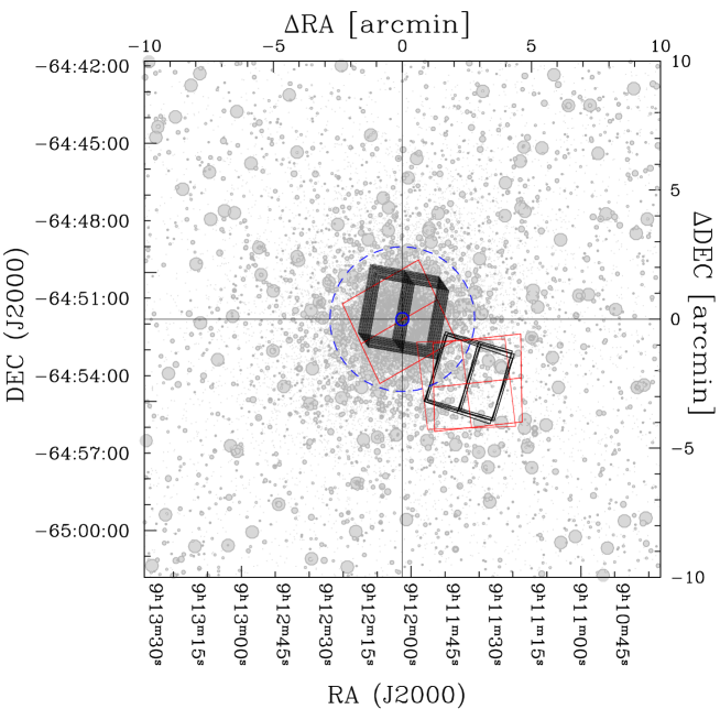
Figure 1: Footprints of the UVIS/WFC3 (black) and WFC/ACS (red) images used in this paper. The circles represented with blue solid and dashed lines indicate the core and the half-light radii of NGC 2808 (from the 2010 version of the Harris, 1996, catalogue).

Ground-based photometry has been used to estimate the atmospheric parameters of the spectroscopic targets while both ground-based and HST photometry are used to identify the stellar populations within NGC 2808 through the ChMs. The $V$ versus ($V-I$) colour-magnitude diagram (CMD) constructed with ground-based photometry is shown in Figure 2.

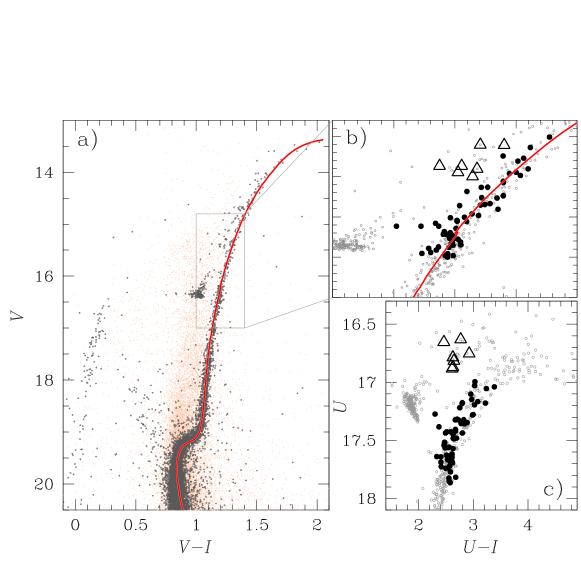
Figure 2: CMDs of stars in the field of view of NGC 2808 based on Stetson et al. (2019) photometry. Panel a shows the differential-reddening corrected $V$ vs. $V-I$ CMD of probable cluster members (grey points) and field stars (orange points). The red line represents the best-fit isochrone from the Dartmouth stellar evolution database (Dotter et al., 2008). We assumed $\rm{[Fe/H]}=-1.17$, $\rm{[}\alpha/\rm{Fe]}=0.40$, $\rm{Age}=12.5$ Gyr, $\rm{E(B-V)}=0.17$ mag and distance modulus, (m$-$M)${}_{0}=14.98$ mag. Panel b and c show a zoom of the panel-a CMD and of the $U$ vs. $U-I$, respectively, around the RGB and the AGB region studied with spectroscopy. The RGB and AGB stars in our spectroscopic sample are indicated as black filled circles and open triangles, respectively.

2.1.1 Chromosome maps

We associated the spectroscopic targets to the five stellar populations identified by Milone et al. (2015), based on their positions in the $\Delta_{C\rm F275W,F336W,F438W}$ vs. $\Delta_{\rm F275W,F814W}$ ChMs derived from stars in the central and external HST fields illustrated in Figure 1.

To associate the stars without HST photometry with the distinct stellar populations we introduced a new ChM that is based on ground-based photometry alone (see also Jang et al. 2022). We used the $I$ vs. $B-I$ CMD, which is sensitive to the helium content of the distinct stellar populations, and the $I$ vs. $C_{\rm U,B,I}$ pseudo-CMD, which separates stellar populations with different nitrogen content. These diagrams are plotted in the panels a and b of Figure 3, where we illustrate the main steps of the procedure to derive the ChM. In a nutshell, we first build the red and blue boundaries of RGB stars in the diagrams of Figure 3a and 3b (see Milone et al., 2015, 2017, for details) and used them to derive the $\Delta_{\rm B,I}$  and $\Delta_{\rm C\,U,B,I}$  pseudo colours of RGB stars. To do this, we adapted to the ground-based photometry the equations by Milone et al. (2017):

$$\Delta_{B,I}=W_{\rm B,I}\frac{X-X_{\rm fiducialR}}{X_{\rm fiducialR}-X_{\rm fiducialB}}$$ (1)

$$\Delta_{C\rm U,B,I}=W_{C\rm U,B,I}\frac{Y-Y_{\rm fiducialB}}{Y_{\rm fiducialR}-Y_{\rm fiducialB}}$$ (2)

where $X=B-I$ and $Y=C_{\rm U,B,I}$ and ‘fiducial R’ and ‘fiducial B’ correspond to the red and the blue fiducial lines, respectively. The adopted values for RGB widths $W_{\rm B,I}$ and $W_{C\rm U,B,I}$ correspond to the colour separation between the RGB boundaries 2.0 $I$ mag above the MS turn off.

The resulting $\Delta_{C\rm U,B,I}$ vs. $\Delta_{\rm B,I}$ is plotted in panel c of Figure 3. In this diagram, the first population (or 1P) stars are clustered around the origin of the ChM, whereas second population (2P) stars define a sequence on the ChM that extends towards large values of $\Delta_{\rm C\,U,B,I}$  and $\Delta_{\rm B,I}$. We refer to the paper by Jang et al. (2022) for extensive discussion of the $\Delta_{\rm C\,U,B,I}$  vs.  $\Delta_{\rm B,I}$  ChM of RGB stars in Galactic GCs.

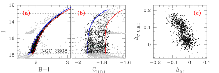
Figure 3: This figure summarises the procedure to derive the ChM from ground based photometry. Panels a and b show the $I$ vs. $B-I$ and the $I$ vs. $C_{\rm U,B,I}$ pseudo CMD, respectively, of probable NGC 2808 cluster members zoomed around the RGB. The red and blue fiducials mark the red and blue RGB boundaries, respectively, while the aqua segments indicates the RGB colour widths. Only the RGB stars between the two horizontal lines and marked with black dots are used to derive the ChM. The resulting $\Delta_{\rm C\,U,B,I}$  vs. $\Delta_{\rm B,I}$  ChM is plotted in panel c.

2.2 Spectroscopic dataset

The initial sample consists of 81 giant stars observed with the spectrograph FLAMES/GIRAFFE (Pasquini et al., 2002) at the Very Large Telescope (observation program 094.D-0455). The stars were observed in two different configurations, the HR4 setup has wavelength coverage from 4188 to 4297 Å  with $\rm{R}\approx 24000$ and the HR18 setup with wavelength coverage from 7468 to 7889 Å  and $\rm{R}\approx 20150$.

We identified 26 stars in the HST ChM, including 24 stars in the central field and 2 in the external field. The ChM derived from ground-based photometry comprises 26 spectroscopic targets.

The data reduction was done using the EsoReflex-based GIRAFFE pipeline (Ballester et al., 2000), which includes bias subtraction, flat-field correction and wavelength calibration. The individual exposures were then corrected to the rest-frame system and eventually combined by using iraf routines. The final signal-to-noise ratio (S/N) of the co-added spectra is $\rm{S/N}\sim 200$.

The list of the observed spectroscopic targets is reported in Table 1, together with coordinates, radial velocities, stellar parameters and chemical abundances obtained as explained in the next sections, and proper motions from Gaia.

Table 1: Right ascension and declination ($J2000$, degrees), radial velocities (km s^-1), proper motions (mas y^-1), effective temperature (K), surface gravity (dex), microturbulence velocities (km s^-1), chemical abundances inferred in this work (dex) for the spectroscopic sample, and a flag indicating the ChM information.

Star	RA	DEC	Vrad	${\mu}_{\alpha,\delta}$	Teff	$\log\rm{g}$	$\xi_{\rm{t}}$	[Fe/H]	[C/Fe]	[N/Fe]	[O/Fe]	[Al/Fe]	[Ni/Fe]	ChM⋆
RGB spectroscopic sample:
N2808_2_36	137.97362	-64.84250	120.7	(1.39,0.05)	4909	2.56	1.28	-1.13	-0.13	0.30	0.56	-0.03	0.19	1
…
AGB spectroscopic sample:
N2808_2_9_wf	137.85825	-64.89367	100.1	(0.95,0.36)	4692	1.97	1.43	-1.20	-0.54	0.43	$<$-0.73	1.01	0.08	0
…

Note. This table is available in its entirety in machine-readable form in the online journal. ^⋆0 for no ChM information, 1 for target in the $HST$ ChM, and 2 for objects in the ground based ChM.

3 Spectroscopic Data Analysis

We derived chemical abundances for cluster stars only. The sample of probable cluster members has been selected based on stellar proper motions and radial velocities (RVs).

We consider proper motions from GAIA eDR3 (Gaia Collaboration et al., 2021). After an inspection of the vector-point diagram of proper motions four stars were identified as outliers and removed from our sample.

The RVs were obtained with the aid of the fxcor task from iraf using a synthetic spectrum template obtained through the March, 2014 version of MOOG (Sneden, 1973). This spectrum was computed with a stellar model atmosphere interpolated from the Castelli & Kurucz (2004) grid, adopting the parameters (T_eff, log g, $\xi_{\rm t}$, [Fe/H]) = (4800 K, 2.5, 1.5 km s^-1, $-$1.2), and cross-correlated with the observed spectra. Each spectrum was corrected to the rest-frame system, and the observed RVs were then corrected to the heliocentric system. The average RV found in our work for NGC 2808 is $102.9\pm 1.1$ km s^-1, in good agreement with the value of $101.6\pm 1.2$ km s^-1 from the 2010 version of Harris (1996).

3.1 Stellar parameters

The stellar parameters effective temperature (T_eff), surface gravity (log g), microturbulent velocity ($\xi_{\rm t}$) and [Fe/H] were, thus, determined for 77 giant stars, including 70 RGB stars and seven AGB stars.

For consistency, the photometry adopted here to determine stellar parameters for all the stars is from ground-based facilities (Stetson et al., 2019). The corresponding $I$ vs. $V-I$ and $U$ vs. $U-I$ CMDs are shown in Figure 2. The effective temperature, $\rm{T}_{\rm{eff}}$, of each star was determined using the ($V-I$), ($V-R$), ($B-V$), ($U-V$), and ($R-I$) colours and the calibration from Alonso et al. (1999), adopting the Bessell (1979) corrections from the Cousins to the Johnson systems. We adopted a reddening of $\rm{E(B-V)}=0.17$ mag and a distance modulus of 14.98 mag, which are the values that best fit the CMD of Figure 2. Our best determination of the effective temperature of each star corresponds to the average of the $\rm{T}_{\rm{eff}}$ values derived from the various colours. The typical standard deviation is 65 K.

We applied bolometric corrections from Alonso et al. (1999) with $\rm{M}=0.85\,\rm{M}_{\odot}$ and the $\rm{T}_{\rm{eff}}$ value calculated from each colour to infer the average $\log g$ value for all the stars (the standard deviation considering the distinct $\log g$ values is 0.03 dex). To infer microturbulence, $\xi_{\rm{t}}$, we used the empirical relation from Marino et al. (2008), where the value $\xi_{\rm{t}}$ depends on stellar gravity.

Finally, we derive the Fe abundance of each star by the equivalent width (EW) method with the aid of the 1D LTE 2014 version of the code moog (Sneden, 1973) and the Kurucz grid of ATLAS9 model atmospheres (Castelli & Kurucz, 2004) with $\rm{[}\alpha/\rm{Fe]}=0.40$. We adopted the line list presented in Table 2, which includes 15 Fe i lines and one Fe ii line from Heiter et al. (2021). The number of lines considered to evaluate [Fe/H] varied from 6 to 16 depending on each star. The internal error associated with the [Fe/H] values was estimated considering the stellar parameters uncertainties as detailed below, and the statistical error from the several lines analysed. The obtained typical [Fe/H] error from our spectra is 0.08 dex (see Table 3).

Table 2: Line list used in the determination of Fe and Ni abundances.

Wavelength (Å)	Species	$\chi_{\rm{exc}}$ (eV)	$\log\rm{gf}$
7491.647	Fe i	4.300	-1.060
7495.066	Fe i	4.220	-0.100
7507.266	Fe i	4.410	-1.470
7511.019	Fe i	4.180	0.119
7531.144	Fe i	4.370	-0.940
7568.899	Fe i	4.280	-0.880
7583.796	Fe i	3.020	-1.880
7586.018	Fe i	4.310	-0.270
7710.363	Fe i	4.220	-1.070
7723.210	Fe i	2.280	-3.580
7748.284	Fe i	2.950	-1.750
7751.109	Fe i	4.990	-0.830
7780.568	Fe i	4.470	-0.090
7807.909	Fe i	4.990	-0.640
7832.196	Fe i	4.430	-0.019
7711.723	Fe ii	3.900	-2.540
7522.758	Ni i	3.655	-0.570
7525.111	Ni i	3.633	-0.550
7555.598	Ni i	3.844	-0.050
7574.043	Ni i	3.830	-0.530
7714.314	Ni i	1.934	-2.200
7727.613	Ni i	3.676	-0.170
7788.936	Ni i	1.949	-2.420
7797.586	Ni i	3.895	-0.260

To identify the presence of possible systematics associated with our analysis, we compared our stellar parameters with the ones obtained by Carretta (2015). Eight out of 77 stars in our sample have been studied in Carretta (2015) as well. We find an average offset of $\Delta\rm{T}_{\rm{eff}}=24\,\rm{K}$ between our values and the $\rm{T}_{\rm{eff}}$ from Carretta (2015), with associated dispersion of 36 K. This difference is probably partially caused by the difference in the method to acquire $\rm{T}_{\rm{eff}}$ as well as the distinct reddening adopted. The largest discrepancy has been obtained for surface gravities, for which our values are $\sim 0.26$ dex higher than the log g by Carretta (2015) and an associated dispersion of 0.03 dex. However, we can explain this difference as mostly due to the distinct distance modulus adopted; Carretta (2015) used a distance modulus of 15.59 (from Harris 1996, 2010 version), and if we consider the same distance modulus the difference between the log g values would decrease to 0.02 dex. Our $\xi_{\rm{t}}$ values agree with those of Carretta and collaborators, being only marginally lower by $\sim 0.12$ km s^-1  with an associated dispersion of 0.10 dex. The difference between our [Fe/H] and the ones of Carretta (2015) shows an average discrepancy of $\sim 0.08$ dex and an associated dispersion of 0.04 dex. The mean discrepancy in the [Fe/H] values is even lower if we consider the difference in the adopted solar constants (in this work we adopted A(Fe)${}_{\odot}=7.50$ from Asplund et al. 2009; while Carretta 2015 adopted A(Fe)${}_{\odot}=7.54$ from Gratton et al. 2003).

This comparison between different datasets suggests that estimates of internal uncertainties associated with our stellar parameters are $\sigma\rm{T}_{\rm{eff}}\sim 50\,\rm{K}$, $\sigma\log\rm{g}\sim 0.10\,\rm{dex}$, $\sigma\xi_{\rm{t}}\sim 0.10\,\rm{km.s}^{-1}$, and $\sigma[\rm{Fe/H}]\sim 0.1\,\rm{dex}$. These uncertainties do not include possible systematics that could be present between our values and the literature ones, such as the systematic difference that we have found in the surface gravities between our values and Carretta (2015).

3.2 Chemical abundances

Beside Fe, we inferred chemical abundances for the light elements C, N, O, Al, and for the iron-peak element Ni. For the light elements we adopted a spectral synthesis analysis using the 1D LTE 2014 version of the code moog (Sneden, 1973) and the Kurucz grid of ATLAS9 model atmospheres (Castelli & Kurucz, 2004) with $\rm{[}\alpha/\rm{Fe]}=0.40$. Figure 4 (panels c, d, e and f) shows the spectral regions adopted to analyse each element.

The heads of the CH G-band ($\rm{A}^{2}\Delta-\rm{X}^{2}II$) at $\sim 4312$ Å  and $\sim 4323$ Å  were used in the C abundances determination by assuming the O abundances determined in this work (as explained below). Nitrogen abundances were inferred from the CN band ($\rm{B}^{2}\Sigma-\rm{X}^{2}\Sigma$) at $\sim 4215$ Å  by assuming both the previously measured O and C abundances.

The triplet in the 7770 Å  region was used to determine the O abundances. Our line list in this spectral region is based on the Kurucz line compendium, with $\log gf$ values of the three O lines from Wiese et al. (1996). The 7771.94 Å  O line was mildly affected by the MgH molecules, which could introduce biases in the O abundances given the large star-to-star Mg variations observed in NGC 2808 (e.g., Pancino et al., 2017; Carretta et al., 2018). Thus, for the O estimates we adopted values from $-$0.2 to 0.4 in [Mg/Fe] for each star according to their Al abundances and the [Al/Fe] vs. [Mg/Fe] anti-correlation from Carretta et al. (2018, see their Figure 3). We also assessed the impact of CN abundances into the O determinations and found that in our stars a change in C and N by $\sim 0.3$ dex affects the abundances from the 7774.17 Å  and 7775.39 Å  lines in the most O-poor stars by as much as 0.2 dex. To avoid the introduction of such systematics due to our assumptions in CN for the most O-poor population, for stars with $\rm{[O/Fe]}\lesssim 0.3$ dex, we infer O abundances from the first triplet line at 7771.94 Å only. The O i 7770 Å  triplet is known to suffer from large departures from LTE (Amarsi et al., 2018), especially towards higher T_eff. To account for this, the abundances inferred from the different components were individually corrected by interpolating the 1D non-LTE grid presented in Amarsi et al. (2019).

Al abundances were obtained by spectral synthesis of the doublet at 7835 Å  region. The line list used in this region was generated by linemake (Placco et al., 2021). Since we want to investigate the [Al/Fe] versus [O/Fe] anti-correlation, the Al abundances were also corrected for departures from LTE, similarly to O abundances discussed above. This was done by interpolating the 1D non-LTE grid of abundances corrections presented in Nordlander & Lind (2017).

Ni was inferred at the same manner as the Fe abundances, e.g. through the assessment of equivalent widths by using the Ni lines listed in Table 2.

An estimate of the final errors associated with our chemical abundances has been derived by determining the variation of each element after the stellar parameters have been changed, once at a time, by their assumed uncertainties (see discussion in the previous section). For the elements obtained through EWs, we also include the statistical error associated with the abundances inferred from the spectral lines that were measured. For the other elements, derived by spectral synthesis, we consider the rms deviation of the observed line profile relative to the synthetic spectra, and the continuum setting. Table 3 lists the contribution of each error source to the final estimated uncertainties due to the internal errors for our inferred abundances. We also list how our chemical abundances change by varying T_eff, log g, $\xi_{\rm t}$ by larger amounts, as possibly due to systematics. We emphasise that our interest is on the internal star-to-star variations in NGC 2808 giants, so that the systematic variations may be considered as a reference when comparing with different analysis.

Table 3: Sensitivity of derived abundances to the uncertainties in the stellar parameters, the signal to noise ($\sigma_{\rm fit}$), abundances of C and O (when applicable), and the subsequent total error ($\sigma_{\rm total}$).

Internal errors
	$\Delta{\rm T}_{\rm eff.}\pm 50\,{\rm K}$	$\Delta\mbox{log~{}{\it g}}\pm 0.10$	$\Delta\xi_{\rm t}\pm 0.10\,\mbox{km~{}s${}^{\rm-1}$}$	$\Delta{\rm[Fe/H]}\pm 0.10$	$\Delta{\rm[O/Fe]}\pm 0.25$	$\Delta{\rm[C/Fe]}\pm 0.20$	$\sigma_{\rm fit}$	$\sigma_{\rm total}$
$[{\rm Fe/H}]$	0.03	0.01	0.03	–	–	–	0.06	0.08
$[{\rm C/Fe}]$	0.03	0.00	0.00	0.07	0.06	–	0.06	0.11
$[{\rm N/Fe}]$	0.08	0.01	0.00	0.05	0.08	0.23	0.11	0.28
$[{\rm O/Fe}]$	0.06	0.04	0.00	0.02	–	–	0.18	0.23
$[{\rm Al/Fe}]$	0.04	0.01	0.01	0.02	–	–	0.15	0.16
$[{\rm Ni/Fe}]$	0.03	0.01	0.04	0.01	–	–	0.10	0.11
Systematic errors
	$\Delta{\rm T}_{\rm eff.}\pm 100\,{\rm K}$	$\Delta\mbox{log~{}{\it g}}\pm 0.30$	$\Delta\xi_{\rm t}\pm 0.30\,\mbox{km~{}s${}^{\rm-1}$}$	$\Delta{\rm[Fe/H]}\pm 0.10$	$\Delta{\rm[O/Fe]}\pm 0.25$	$\Delta{\rm[C/Fe]}\pm 0.20$	$\sigma_{\rm fit}$	$\sigma_{\rm total}$
$[{\rm Fe/H}]$	0.07	0.01	0.09	–	–	–	0.06	0.13
$[{\rm C/Fe}]$	0.07	0.02	0.00	0.07	0.06	–	0.06	0.13
$[{\rm N/Fe}]$	0.17	0.05	0.00	0.05	0.08	0.23	0.11	0.32
$[{\rm O/Fe}]$	0.12	0.10	0.01	0.02	–	–	0.18	0.25
$[{\rm Al/Fe}]$	0.04	0.01	0.01	0.02	–	–	0.15	0.17
$[{\rm Ni/Fe}]$	0.07	0.04	0.10	0.01	–	–	0.10	0.16

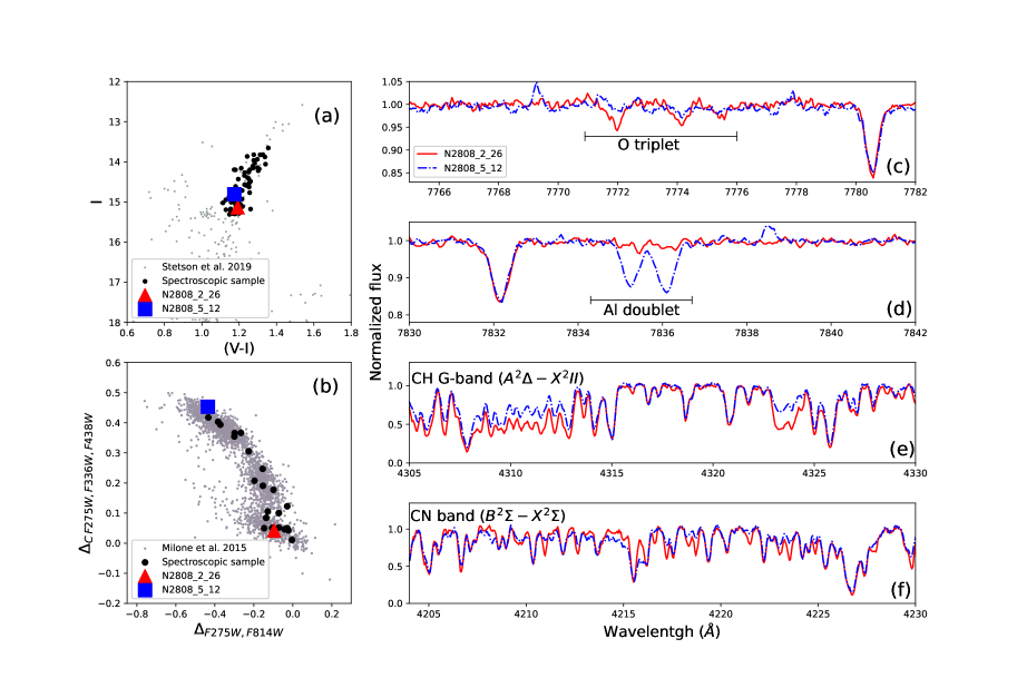
Figure 4: Comparison between two stars with similar photometry (panel a) but from different populations according to their ChM position (panel b). Red solid lines show the spectra of N2808_2_26 ($\mbox{T${}_{\rm eff}$}=4909$ K, $\mbox{log~{}{\it g}}=2.56$, $\mbox{$\xi_{\rm t}$}=1.28$ km s^-1, $\rm{[Fe/H]}=-1.13$) and the dashed blue lines represent the spectra of N2808_5_12 ($\mbox{T${}_{\rm eff}$}=4893$ K, $\mbox{log~{}{\it g}}=2.44$, $\mbox{$\xi_{\rm t}$}=1.31$ km s^-1, $\rm{[Fe/H]}=-1.12$) for four distinct regions of their spectra: O triplet at 7770 Å  (panel c), Al doublet at 7835 Å  (panel d), CH G-band $\rm{A}^{2}\Delta-\rm{X}^{2}II$ (panel e) and CN band $\rm{B}^{2}\Sigma-\rm{X}^{2}\Sigma$ (panel f).

The final abundances of the element “X” obtained in our study are shown as $\rm{[X/Fe]}=\rm{A}(\epsilon_{\rm{X}\star})-\rm{A}(\epsilon_{\rm{X}\odot})-\rm{[Fe/H]}$, where $\rm{A}(\epsilon_{\rm{X}\star})=\log\rm{N(X)}/\rm{N(H)}+12$ is the absolute abundance of a star and $\rm{A}(\epsilon_{\rm{X}\odot})$ is the solar photospheric abundances values from Asplund et al. (2009).

4 Results and discussion

The astrometric positions, stellar parameters and chemical abundances inferred in this work are listed in Table 1. The table is divided into RGB and AGB stars.

In the following subsections we discuss the general chemical abundances of RGB and AGB stars in NGC 2808, and finally we present the analysis of the chemical patterns associated to the distinct stellar populations as observed on the ChM.

4.1 The chemical composition of RGB stars

In Figure 5 we show the histogram distribution of [Fe/H]. Our analysed stars have a mean iron content of $\rm{[Fe/H]}=-1.05\pm 0.01$. The associated dispersion of 0.07 dex, very similar to the estimated error of 0.08 dex, suggests that our sample of stars is consistent with an homogeneous Fe distribution.

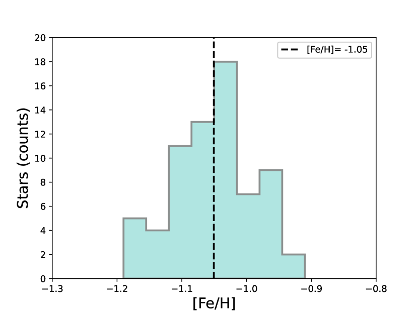
Figure 5: [Fe/H] distribution for the 70 RGB stars in our sample. The black dashed line indicates the average [Fe/H] value.

As expected for Milky Way GCs, the chemical content of the light elements C, N, O and Al, involved in the high-temperature $p$-capture reactions, differs from star to star (e.g., Gratton et al., 2004). The variation of this set of elements is visualised in Figure 4, which presents the comparison of two stars with similar atmospheric parameters (panel a) but from different populations, according to the location on the ChM (panel b). According to the classification of Milone et al. (2015), the two represented stars, namely N2808_2_26 (red triangle) and N2808_5_12 (blue square) belong to populations B and D, respectively. They show different abundances of C (panel e), N (panel f), O (panel c) and Al (panel d), that can be easily identified by eye from a quick inspection of their spectra.

Specifically, for our spectroscopic sample of RGB stars, the [O/Fe] varies from $\lesssim-0.73$ to $+0.73$ dex with an average value of $\rm{[O/Fe]}=0.13\pm 0.05$ and an associated dispersion of 0.42 dex. [C/Fe] abundances range from $-0.93$ to $0.02$ with an average value of $\rm{[C/Fe]}=-0.42\pm 0.03$ and an associated dispersion of 0.26 dex. [N/Fe] abundances vary from $-0.50$ to $1.35$ with an average of $\rm{[N/Fe]}=0.74\pm 0.06$ and an associated dispersion of 0.49 dex. The values of [Al/Fe] go from $-0.24$ to $1.14$ with average abundance of $\rm{[Al/Fe]}=0.38\pm 0.06$ and an associated dispersion of 0.46 dex. Differently, [Ni/Fe] has a smaller variation, ranging from $-0.05$ to $0.25$ dex, with average abundance of $\rm{[Ni/Fe]}=0.08\pm 0.01$ and associated dispersion of 0.06 dex.

The expected (anti-)correlations of [C/Fe] with [N/Fe], and [Al/Fe] with [O/Fe] are shown in Figure 6. For comparison purposes, we also show [Ni/Fe] and [Fe/H] abundances versus [O/Fe]. The classical anti-correlation between [N/Fe] and [C/Fe] is presented in the top right panel.

The variations in the abundances from C, N, O and Al show the intense interplay in the production and destruction of these elements in the different objects in NGC 2808. As a product of the CNO cycle, during hot hydrogen burning, C and O are reduced while N is highly enhanced. At the same time, Al is produced through the Mg-Al chain (Arnould et al., 1999; Karakas & Lattanzio, 2003). Meanwhile, [Ni/Fe] is constant with [O/Fe], and also constant in the different populations (see discussion in §  4.4).

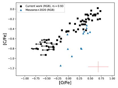
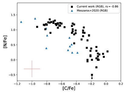
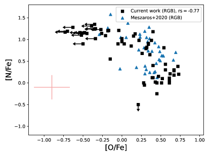
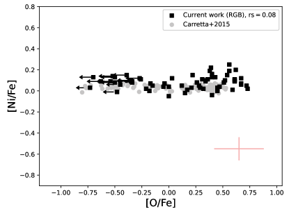
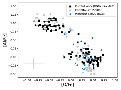
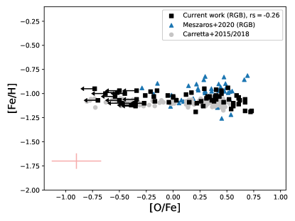
Figure 6: Abundances obtained in the current work for RGB stars (black squares) compared to data from Mészáros et al. (2020) (blue triangles) and Carretta (2015); Carretta et al. (2018) (grey circles). Top left panel shows [C/Fe] vs. [O/Fe], top right panel presents [N/Fe] vs. [C/Fe], [N/Fe] vs. [O/Fe] is in the left middle panel, [Ni/Fe] vs. [O/Fe] is presented in the right middle panel, [Al/Fe] vs. [O/Fe] is shown in the bottom left panel and [Fe/H] vs. [O/Fe] is in the bottom right panel. The typical error (mean value) is displayed in red. The Spearman coefficients ($rs$) for each possible (anti-)correlation are reported in all panels.

For our sample of stars with the full set of C, N, and O abundances available (excluding the upper limits), we find an average C$+$N$+$O overall abundance of $\rm{A(C+N+O)}=8.16\pm 0.02$ with associated dispersion of 0.10 dex. We also notice that the overall C$+$N$+$O content slightly decreases when moving from first-population stars to populations C and D.

However, we notice that values of A(C$+$N$+$O) may be significantly affected by systematic uncertainties of the absolute abundances of C, N, and O. To estimate the robustness of our C$+$N$+$O abundances, we estimated the variations in A(C$+$N$+$O) that we obtain by changing C, N, O, individually. To do this, we varied each element at time by an amount corresponding to its internal uncertainty (Table 3). We find that the C$+$N$+$O content is not significantly affected by systematic errors in C. On the contrary, N and O variations correspond to significant C$+$N$+$O changes, which may have different effectes on the different stellar populations. Specifically, a systematic variation of N by 0.28 dex mostly affect Populations C and D stars, with the latter varying up to $\sim$0.2 dex. Systematic errors in O mostly affect the most O-rich populations, (i.e. the 1P). An oxygen variation by $\pm 0.23$ dex, corresponds to a C$+$N$+$O increase by $\sim$0.2 dex in Population 1 stars, to a decrease by $\sim$0.1 dex and $\sim$0.05 in Population C and D, respectively. We conclude that the relative C$+$N$+$O content of the distinct stellar populations is significantly affected by systematic errors in the C, N, and O determinations. This fact prevents us from firm conclusion on C$+$N$+$O variations among the distinct stellar populations of NGC 2808.

4.2 The chemical composition of AGB stars

Our spectroscopic sample comprises seven probable AGB stars, as clearly suggested by the location of these stars in the $U$ vs. ($U-I$) CMD (see Figure 2). In this sample, all the analysed light elements show a significant range, specifically: [O/Fe] vary from $\lesssim-0.73$ to $0.83$ dex with an average value of $\rm{[O/Fe]}=0.37\pm 0.21$ dex (associated dispersion of 0.52 dex); [C/Fe] abundances range from $-0.98$ to $-0.25$ dex and average value of $\rm{[C/Fe]}=-0.47\pm 0.10$ dex (associated dispersion of 0.25 dex); [N/Fe] varies from $+0.40$ to $+1.17$ dex with an average abundance of $\rm{[N/Fe]}=+0.64\pm 0.10$ dex (associated dispersion of 0.25 dex); and [Al/Fe] values range from $-0.25$ to $1.01$ dex with average abundance of $\rm{[Al/Fe]}=0.16\pm 0.19$ dex (associated dispersion of 0.46 dex). Additionally, similar to the RGB sample, [Ni/Fe] abundances span a smaller range from $-0.04$ to $0.13$ dex, with average abundance of $\rm{[Ni/Fe]}=0.05\pm 0.02$ dex and dispersion of 0.06 dex.

The abundances of our AGB stars in comparison with the results for RGB are shown in Figure 7. For completeness, we show results from AGB stars by Mészáros et al. (2020). An inspection of the [N/Fe] (middle left), [Ni/Fe] (middle right), [Al/Fe] (bottom left) and [Fe/H] (bottom right) versus [O/Fe] plots indicates that those stars have similar abundances when compared to the RGB stars in our sample. However, the upper panels of Figure 7 ([C/Fe] versus [O/Fe] and [N/Fe] versus [C/Fe]) might indicate that our AGB stars have lower content of C, in general, when compared to the RGB sample (by a factor of $\sim 1.1$). This behaviour could be related to the different evolutionary stage of the AGB stars. In particular the C $\to\,{\rm{N}}$ processing occurring in the RGB envelopes could modify the CN surface abundances on the AGB (e.g., Smith & Norris, 1993).

From the Al-O anti-correlation presented in Figure 7, we observe AGB stars belonging to both first and second populations, in agreement with Marino et al. (2017) in the same cluster. Interestingly enough, we note that the O abundance inferred for one star is very low, with none of such extremely-O depleted stars, possibly associated to the population E on the ChM, included in the sample of Marino et al. (2017). This star (N2808_2_9_wf) also displays high [Al/Fe], which is compatible with the star belonging to the extremely-helium rich population. On the other hand, we note that this object has more [C/Fe] and less [N/Fe] content than what is expected for the extremely-He enriched stellar population.

We regard this star as an interesting target for future observations with higher-resolution spectroscopy. Indeed, the stars with the highest content of He (D’Antona et al., 2005; Milone et al., 2015) would in principle avoid the AGB phase becoming AGB-manqué stars (Greggio & Renzini, 1990; Gratton et al., 2010; Chantereau et al., 2016). Nonetheless, Marino et al. (2017) detected an AGB star with the same chemical composition as population-D stars. This finding demonstrates that NGC 2808 stars with Y$\sim$0.3 can evolve to the AGB phase; in addition, Lagioia et al. (2021) found that several AGB stars can be associated with population D and possibly population E, based on their positions on the ChM. These findings might challenge the current stellar evolution models (Chantereau et al., 2016).

The evidence that He-rich stars in GCs skip the AGB phase and evolve as AGB manqué, together with the presence of extremely blue He-rich HB stars, makes it tempting to link the phenomenon of multiple stellar populations with the X-UV Upturn phenomenon of elliptical galaxies. The latter consists of a ‘UV rising branch’ at wavelengths shorter than $\lambda\lesssim 2500$ Å  observed in the spectra of elliptical galaxies (e.g., Code 1969), whose origin is still controversial. By far, AGB manqué stars and extreme HB stars are considered among sources that are likely to produce the largest contribution to the UV output from a galaxy (e.g., Renzini 1990). Hence, if elliptical galaxies host multiple stellar populations, similar to GCs, it is possible that helium-rich stars are responsible for the X-UV upturn phenomenon.

Recent works have provided robust evidence of a significant amount of AGB manqué stars, among He-rich GC stars (e.g., Campbell et al. 2013, Marino et al. 2017 and Lagioia et al. 2021). The discovery of a He-rich AGB star would certainly indicate that a small fraction of AGB He-rich stars skip the AGB phase. However, a large statistic sample of He-rich AGB stars is needed to estimate their fraction and their contribution to the total X-UV flux of a GC.

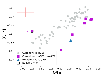
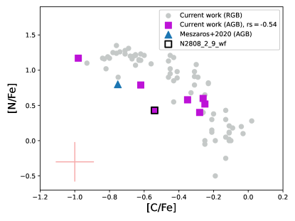
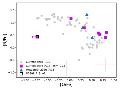
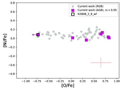
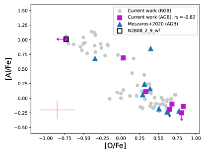
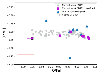
Figure 7: Abundances for AGB stars obtained in the current work (purple squares) compared to AGB stars from Mészáros et al. (2020) (blue triangles) and our study of RGB stars (light grey circles). Top left panel shows [C/Fe] vs. [O/Fe], top right panel presents [N/Fe] vs. [C/Fe], [N/Fe] vs. [O/Fe] is in the left middle panel, [Ni/Fe] vs. [O/Fe] is presented in the right middle panel, [Al/Fe] vs. [O/Fe] is shown in the bottom left panel and [Fe/H] vs. [O/Fe] is in the bottom right panel. The typical error (mean value) is displayed in red. The Spearman coefficients ($rs$) for each possible (anti-)correlation are reported in all panels.

4.3 Literature comparison

Several studies of the chemical abundances in NGC 2808 can be found in the literature, so it is worth discussing here a comparison with previous results. The most recent studies by Carretta (2015) and Carretta et al. (2018) include the [O/Fe], [Al/Fe] and [Ni/Fe] abundances. In addition, Mészáros et al. (2020) presented [C/Fe], [N/Fe], [O/Fe] and [Al/Fe] abundances, based on APOGEE spectra.

Our average [Fe/H] for NGC 2808 is $-1.05$ dex with a dispersion of 0.07 dex (considering only RGB stars). This value is 0.09 dex higher than the one reported in Harris (1996) (2010 version, [Fe/H]$=-1.14$ dex that is an average result compiled with values found in the literature), 0.08 dex greater than the [Fe/H] average from Carretta (2015) ([Fe/H]$=-1.13$ dex) but if we consider the same solar constant for Fe the difference decreases to 0.04 dex, and 0.12 dex smaller than the average metallicity from Mészáros et al. (2020) ([Fe/H]$=-0.93$ dex) and again, if we consider the same Fe solar constant the difference diminishes to 0.07 dex.

Figures 6 and 7 show the literature comparison for the (anti-) correlations between [C/Fe], [N/Fe], [Al/Fe] and [O/Fe], as well as [Ni/Fe] versus [O/Fe] and [Fe/H] versus [O/Fe] for RGB and AGB stars, respectively. The classical anti-correlation between [C/Fe] and [N/Fe] and their comparison with literature studies is also shown. For a better comparison, the abundances from Carretta (2015); Carretta et al. (2018) and Mészáros et al. (2020) presented in these figures are also corrected to the same solar constants used in our work.

Although the methods and spectral regions used to analyse the chemical abundances of different elements from Carretta (2015), Carretta et al. (2018) and Mészáros et al. (2020) are distinct from our work, we found a reasonable concordance of our findings when compared to these studies. Carretta (2015) used the [O i] forbidden lines at $\sim 6300$ Å  and several Ni i lines from 4900 to 6800 Å. For Al determination, Carretta et al. (2018) used the method presented in Carretta et al. (2012) that analysed the Al i doublet at 8772-73 Å. Lastly, Mészáros et al. (2020) used infrared features to determine the abundances of Al, C, N and O.

Our RGB C abundances are higher than the ones from Mészáros et al. (2020) by a factor of $\sim 1.3$, while the N from Mészáros et al. (2020) are higher than our results by a factor of $\sim 1.7$. We analysed RGB stars that are below or above the luminosity bump (with magnitudes in the interval $15.0\lesssim V\lesssim 16.6$) while Mészáros et al. (2020) only have stars above the RGB bump (with stars as bright as $V\sim 13.5$), so a mild difference is expected. Although we have stars both below and above the RGB bump, our abundances of [C/Fe] and [N/Fe] do not show any trend with luminosity; probably because our sample does not include very bright RGB stars.

4.4 Chemical abundances along the ChMs

The upper panels of Figure 8 show the ChMs of NGC 2808 from HST and ground based photometry. The spectroscopic sample is colour-coded according to their populations based on the classification in Milone et al. (2015). In the following, we investigate the chemical composition of four stellar populations: the first population 1P, and the three main groups of second-population stars, namely C, D, and E. Figure 8 shows [N/Fe] (bottom left panel) and [Al/Fe] (bottom right panel) versus [O/Fe] for the sample of RGB stars and the highlighted stars for which we have ChM information.

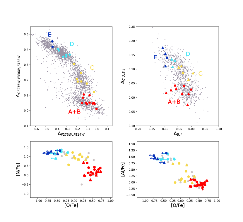
Figure 8: The upper panels shows the HST ChM from the two field of view shown in Figure 1 that include data from Milone et al. (2015) (left) and our ChM from ground based photometry (right), with the spectroscopic data divided in populations A+B (red), C (yellow), D (cyan) and E (dark blue). [N/Fe] (bottom left panel) and [Al/Fe] (bottom right panel) versus [O/Fe] for our RGB sample (grey circles) with the populations colour coded in agreement with the ChM panels. Spectroscopic data with HST ChM information are represented with filled circles, while filled triangles show spectroscopic data with ground based ChM information.

N is the most sensitive element (presented in our work) for the location of a star in the ChM, as shown by Marino et al. (2019a). Due to the filters used in the construction of a ChM, variations in N would translate in a different position for the stars in this diagram. Oxygen variation also affect, to a minor extent, the position of a star along the ChM. Thus, in our study, the [N/Fe] versus [O/Fe] plot is an efficient tool to analyse multiple populations in a GC with spectroscopic data. The left bottom panel of Figure 8 shows this anti-correlation and the clear separation between 1P stars and Population C stars. Populations D and E share similar N contents, whereas the most extreme star from population E present the lowest O abundances. We note a clear separation among the distinct populations also in the right bottom panel of Figure 8, which shows the anti-correlation of [Al/Fe] versus [O/Fe].

Table 4 summarises the average abundances of each element studied here for each ChM population, both for HST and ground based photometry. [Fe/H] is constant in the distinct populations, at a level of $\lesssim$0.10 dex. The abundances of [C/Fe] and [O/Fe] decrease from 1P (i.e. Populations A$+$B) stars to E, while [N/Fe] and [Al/Fe] abundances increase. Except for O and Li, which are substantially lower in the E population with respect to population D stars, we do not observe large differences in the other light elements between these two stellar populations.

Table 4: Average abundances for each population of stars, with their respective mean errors, dispersion ($\sigma$), and number of stars (#).

Current work
	Pop. A+B	$\sigma$	#	Pop. C	$\sigma$	#	Pop. D	$\sigma$	#	Pop. E	$\sigma$	#
$\left\langle\rm{[Fe/H]}\right\rangle$	$-1.07\pm 0.02$	0.07	20	$-1.04\pm 0.01$	0.04	12	$-1.05\pm 0.02$	0.06	10	$-1.02\pm 0.02$	0.06	6
$\left\langle\rm{[C/Fe]}\right\rangle$	$-0.16\pm 0.02$	0.08	20	$-0.40\pm 0.03$	0.09	12	$-0.68\pm 0.02$	0.05	10	$-0.72\pm 0.03$	0.07	6
$\left\langle\rm{[N/Fe]}\right\rangle$	$0.21\pm 0.05$	0.23	19	$0.95\pm 0.05$	0.17	12	$1.17\pm 0.04$	0.11	10	$1.22\pm 0.02$	0.06	6
$\left\langle\rm{[O/Fe]}\right\rangle$	$0.51\pm 0.03$	0.14	20	$0.09\pm 0.05$	0.17	12	$\lesssim-0.39$	0.14	8	$\lesssim-0.58$	0.14	5
$\left\langle\rm{[Al/Fe]}\right\rangle$	$-0.05\pm 0.02$	0.09	20	$0.28\pm 0.08$	0.28	12	$0.90\pm 0.03$	0.08	10	$0.95\pm 0.05$	0.12	6
$\left\langle\rm{[Ni/Fe]}\right\rangle$	$0.08\pm 0.02$	0.08	20	$0.06\pm 0.02$	0.07	12	$0.06\pm 0.02$	0.05	10	$0.09\pm 0.02$	0.04	6
Literature data$\dagger$
	Pop. A+B	$\sigma$	#	Pop. C	$\sigma$	#	Pop. D	$\sigma$	#	Pop. E	$\sigma$	#
$\left\langle\rm{[Fe/H]}\right\rangle$	$-1.12\pm 0.01$	0.02	27	$-1.12\pm 0.01$	0.02	14	$-1.10\pm 0.01$	0.01	4	$-1.11\pm 0.01$	0.02	6
$\left\langle\rm{A(Li)}\right\rangle$	$1.16\pm 0.02$	0.05	5	$1.10\pm 0.03$	0.08	6	$1.05\pm 0.02$	0.05	6	$0.82\pm 0.11$	0.16	3
$\left\langle\rm{[O/Fe]}\right\rangle$	$0.27\pm 0.02$	0.09	25	$-0.16\pm 0.08$	0.30	11	$-0.35\pm 0.11$	0.19	3	$-0.46\pm 0.07$	0.16	2
$\left\langle\rm{[Na/Fe]}\right\rangle$	$0.02\pm 0.02$	0.08	27	$0.32\pm 0.03$	0.12	14	$0.39\pm 0.04$	0.06	4	$0.44\pm 0.04$	0.10	6
$\left\langle\rm{[Mg/Fe]}\right\rangle$	$0.37\pm 0.01$	0.05	27	$0.27\pm 0.03$	0.11	14	$0.12\pm 0.07$	0.12	4	$0.09\pm 0.06$	0.14	6
$\left\langle\rm{[Al/Fe]}\right\rangle$	$-0.08\pm 0.04$	0.18	21	$0.72\pm 0.13$	0.47	9	$1.09\pm 0.04$	0.08	4	$1.13\pm 0.09$	0.21	6
$\left\langle\rm{[Si/Fe]}\right\rangle$	$0.27\pm 0.01$	0.03	27	$0.31\pm 0.01$	0.04	14	$0.34\pm 0.02$	0.03	4	$0.36\pm 0.02$	0.05	6
$\left\langle\rm{[Ca/Fe]}\right\rangle$	$0.32\pm 0.01$	0.03	27	$0.33\pm 0.01$	0.02	14	$0.32\pm 0.01$	0.02	4	$0.32\pm 0.01$	0.03	6
$\left\langle\rm{[Sc/Fe]}\right\rangle$	$-0.03\pm 0.01$	0.04	27	$0.01\pm 0.01$	0.04	14	$0.01\pm 0.01$	0.03	4	$0.05\pm 0.01$	0.02	6
$\left\langle\rm{[Ti/Fe]}\right\rangle$	$0.22\pm 0.01$	0.04	27	$0.21\pm 0.01$	0.02	14	$0.211\pm 0.01$	0.02	4	$0.18\pm 0.01$	0.03	6
$\left\langle\rm{[Cr/Fe]}\right\rangle$	$-0.04\pm 0.01$	0.03	27	$-0.03\pm 0.01$	0.03	14	$-0.03\pm 0.01$	0.01	4	$-0.01\pm 0.01$	0.01	6
$\left\langle\rm{[Mn/Fe]}\right\rangle$	$-0.38\pm 0.01$	0.01	5	$-0.36$	–	1	$-0.38$	–	1	$-0.40$	–	1
$\left\langle\rm{[Ni/Fe]}\right\rangle$	$-0.07\pm 0.01$	0.02	27	$-0.07\pm 0.01$	0.02	14	$-0.07\pm 0.02$	0.03	4	$-0.07\pm 0.01$	0.02	6

Note. $\dagger$Data from Carretta (2015), Carretta et al. (2018) and D’Orazi et al. (2015).

Figure 9 shows the same (anti-)correlations presented in Figure 6, but now with the average abundances for each population of the ChM illustrated by coloured circles (red for population A+B, C in yellow, D in cyan and dark blue for population E). We find distinct average abundances for the different stellar populations, with population E (blue circles) showing the lowest O abundances (with some stars having only upper limits).

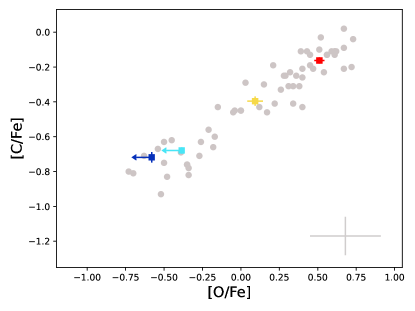
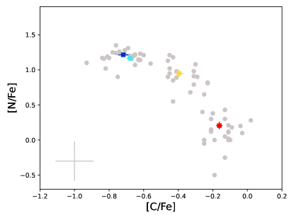
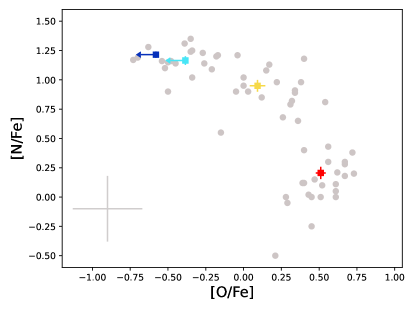
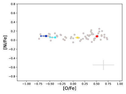
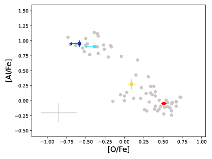
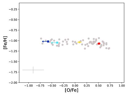
Figure 9: Abundance panels for RGB stars (grey circles) with their average abundances for each population highlighted. Population A+B is represented by red squares, the yellow squares illustrate population C, averages for population D are shown as cyan squares and dark blue squares display values for population E. Top left panel shows [C/Fe] vs. [O/Fe], top right panel presents [N/Fe] vs. [C/Fe], [N/Fe] vs. [O/Fe] is in the left middle panel, [Ni/Fe] vs. [O/Fe] is presented in the right middle panel, [Al/Fe] vs. [O/Fe] is shown in the bottom left panel and [Fe/H] vs. [O/Fe] is in the bottom right panel.

To further analyse the chemical abundances along the ChM of NGC 2808, in Figures 10 and 11 we plot the chemical abundances as a function of the $\Delta_{\tiny{C~{}\mathrm{F275W,F336W,F438W}}}$ (from $HST$ photometry) and $\Delta_{\rm C\,U,B,I}$ (from ground-based photometry) values, respectively.

Carbon and oxygen both show a strong anti-correlation with $\Delta_{\tiny{C~{}\mathrm{F275W,F336W,F438W}}}$, with Spearman coefficients $r_{S}=-0.92$ and $r_{S}=-0.88$, respectively; which indicates that 1P stars, located at lower values of $\Delta_{\tiny{C~{}\mathrm{F275W,F336W,F438W}}}$, have higher content of these elements. On the other hand, [N/Fe] and [Al/Fe] are positively correlated with $\Delta_{\tiny{C~{}\mathrm{F275W,F336W,F438W}}}$, with Spearman coefficients equal to $+0.94$ and $+0.93$, meaning that A+B stars have less [N/Fe] and [Al/Fe] in comparison with populations C, D and E stars. Meanwhile, [Ni/Fe] and [Fe/H] do not present any (anti-)correlation with $\Delta_{\tiny{C~{}\mathrm{F275W,F336W,F438W}}}$ (Spearman coefficients $r_{S}=0.07$ and $r_{S}=-0.25$, respectively) which indicates that there are no variations of those abundances, within our uncertainties, through the different populations hosted in NGC 2808.

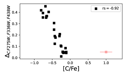
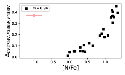
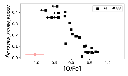
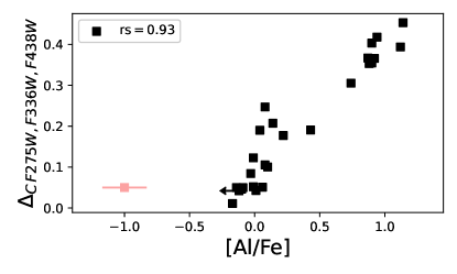
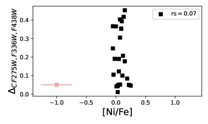
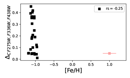
Figure 10: $\Delta_{\tiny{C~{}\mathrm{F275W,F336W,F438W}}}$ versus [C/Fe] (top left panel), [N/Fe] (top right panel), [O/Fe] (middle left panel), [Al/Fe] (middle righgt panel), [Ni/Fe] (bottom left panel) and [Fe/H] (bottom right panel). The typical errors are marked in red.

The ground-based ChM show a similar behaviour. Figure 11 displays $\Delta_{\rm C\,U,B,I}$  versus [C/Fe], [N/Fe], [O/Fe], [Al/Fe], [Ni/Fe], and [Fe/H]. [C/Fe] and [O/Fe] show strong anti-correlation with $\Delta_{\rm C\,U,B,I}$, with their respective Spearman coefficients being $r_{S}=-0.90$ and $r_{S}=-0.82$. [N/Fe] and [Al/Fe] have prominent correlation with $\Delta_{\rm C\,U,B,I}$, with $r_{S}=+0.91$ and $r_{S}=+0.89$, respectively; demonstrating once more the strong dependency of the light elements with the location on the $y$ axis of the ChM. Analogous to the result shown in Figure 10, the bottom panels of Figure 11 show the weak (or no) correlation of [Ni/Fe] and [Fe/H] with $\Delta_{\rm C\,U,B,I}$, corroborating that there are no significant variations of those abundances through the different populations of NGC 2808.

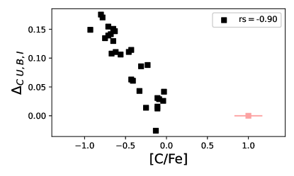
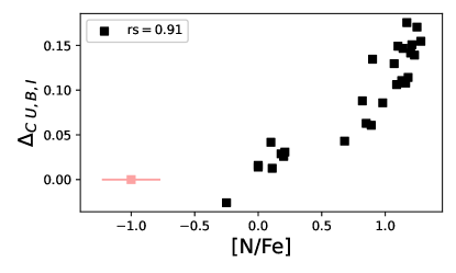
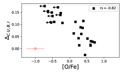
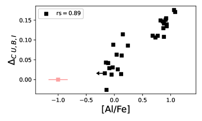
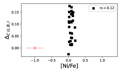
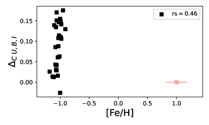
Figure 11: $\Delta_{\rm C\,U,B,I}$ versus [C/Fe] (top left panel), [N/Fe] (top right panel), [O/Fe] (middle left panel), [Al/Fe] (middle right panel), [Ni/Fe] (bottom left panel) and [Fe/H] (bottom right panel). The typical errors are marked in red.

The agreement between the relations of each analysed element with the ChM values shown in Figures 10 and 11 for $HST$ and ground-based photometry, respectively, demonstrates the effectiveness of the ChM constructed from ground based photometry in separating the stellar populations in GCs. The combined efforts from both $HST$ and ground based ChMs is an important tool to analyse the multiple population phenomenon in GCs over a wide field of view.

For a complete assessment of chemical variations along the ChMs, we assemble literature high resolution spectroscopic data and combine them with the recent information from our new ground based ChM. Lithium is a crucial element to understand multiple populations. As it is easily destroyed by proton-capture in stellar environments, the observed abundances for this element depend on the interplay between several mechanisms that can decrease the internal and surface Li content of low-mass stars at different phases of their evolution. The Li abundances along the ChM of NGC 2808 has been discussed in Marino et al. (2019a) by using the ChM from HST photometry and Li abundances from D’Orazi et al. (2015). They found lithium abundances only slightly changing from one population to another, with one population-E star being depleted in lithium by only $\sim$0.2 dex with respect to 1P stars.

We take advantage of our newly-introduced ground-based ChM to investigate the Li abundances along this diagram. The D’Orazi et al. (2015) sample includes 12 stars with available ChM position from the large field of view of the ground-based photometry, plus 8 stars from the two $HST$ fields of view. Since these stars are in a similar evolutionary stage, we are able to compare the [Al/Fe] and A(Li) according to their distinct populations. These stars are below the RGB bump, hence they do not experience yet extra mixing that induce another event of severe depletion in the Li content (e.g., Charbonnel & Zahn, 2007), the first strong episode of Li dilution occurs during the first dredge-up. Figure 12 shows the A(Li) versus [Al/Fe] plot, using abundances from D’Orazi et al. (2015), with the average values for each population highlighted. We observe the majority of 1P stars showing lower content of Al and slightly higher Li than 2P stars. Most stars of population C have low Al, and Li similar to population D stars. The three population E stars display high Al abundances and the lowest Li content. This result is in agreement with Marino et al. (2019a) for stars in the $HST$ ChM.

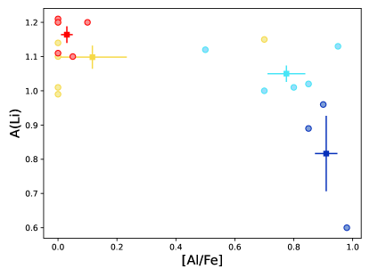
Figure 12: [Al/Fe] versus NLTE A(Li) from D’Orazi et al. (2015) with the corresponding population tagging according to our $HST$ and ground based ChMs (circles) compared to their averages abundances (squares).

We also compile the abundances from Carretta (2015) and Carretta et al. (2018) that have ChM information. Table 4 and Figure 13 summarises the average chemical abundances from Carretta (2015); Carretta et al. (2018); D’Orazi et al. (2015), in addition to our results, separated by the populations marked in the ChM.

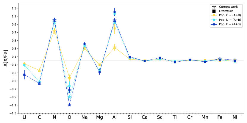
Figure 13: Average chemical abundances from stars in populations C (yellow), D (cyan) and E (dark blue) with respect to the 1P (A+B), with our results (open stars) and data from Carretta (2015), Carretta et al. (2018) and D’Orazi et al. (2015) (filled squares). All elements have $\Delta$[X/Fe] reported, with the exception of lithium ($\Delta$A(Li)) and iron ($\Delta$[Fe/H]).

Following the outcome from our spectroscopic analysis, the literature chemical abundances from light elements, O, Na, Mg and Al , are the most sensitive to distinct ChM populations, while Si and Sc have little changes, and Ti and the iron peak elements, Cr, Mn, Fe, and Ni, present negligible variation within the different populations.

Finally, we compare our C, N and O abundances for which we have $HST$ ChM information to the [C/Fe], [N/Fe] and [O/Fe] values by Milone et al. (2015) inferred from a photometric analysis based on the comparison between the observed diagrams with stellar models and synthetic spectra. The average abundances of each element in a given population are listed in Table 5 with respect to population B. In our work, we did not separate populations A and B, although one star with $HST$ ChM information being consistent with population A, namely N2808_1_8_0. For the sake of information, we report for this star abundances of: [Fe/H]$=-0.95$ (marginally higher than the average 1P value), [C/Fe]$=-0.25$, [N/Fe]$=-0.05$ and [O/Fe]$=+0.29$.

The comparison between our average chemical abundances and the ones from Milone et al. (2015) shows that:

• we have more moderate values of $\Delta\rm{[C/Fe]}$, while Milone et al. (2015) presented more extreme values for these quantities in populations D and E, though being compatible for population C;

• our results for $\Delta\rm{[N/Fe]}$ are compatible with the work of Milone et al. (2015) for populations C, D and E;

• differently, our $\Delta\rm{[O/Fe]}$ are substantially larger than the ones from Milone et al. (2015).

Results from Milone et al. (2015) are entirely based on multi-band photometry. The comparison between the N abundance from spectroscopic- and photometric-based analysis demonstrates that photometry is an excellent tool to assess the content of this element, which, together with helium, is the element that most affects the location of a star on the ChM. Our comparison shows that photometry allows to qualitatively distinguish stellar populations with different abundances of C and O.

Table 5: [C/Fe], [N/Fe] and [O/Fe] abundances for each population with respect to 1P stars.

	Our work
Population	$\Delta\rm{[C/Fe]}$	$\Delta\rm{[N/Fe]}$	$\Delta\rm{[O/Fe]}$
A+B	0.0	0.0	0.0
C	$-0.21\pm 0.03$	$0.66\pm 0.10$	$-0.45\pm 0.06$
D	$-0.50\pm 0.03$	$0.96\pm 0.07$	$-0.81\pm 0.07$
E	$-0.56\pm 0.06$	$0.98\pm 0.08$	$-1.04\pm 0.15$
	Milone et al. (2015)
Population	$\Delta\rm{[C/Fe]}$	$\Delta\rm{[N/Fe]}$	$\Delta\rm{[O/Fe]}$
A	$0.2\pm 0.2$	$0.0\pm 0.1$	$0.2\pm 0.1$
B	0.0	0.0	0.0
C	$-0.1\pm 0.1$	$0.6\pm 0.2$	$0.0\pm 0.1$
D	$-0.8\pm 0.3$	$1.1\pm 0.1$	$-0.5\pm 0.1$
E	$-0.9\pm 0.3$	$1.2\pm 0.2$	$-0.7\pm 0.1$

5 summary and conclusions

This work investigates multiple stellar populations along the RGB and the AGB of NGC 2808 by combining information from different techniques. We use the multi-band HST photometry and proper motions for stars in the $\sim 2.7\times 2.7$ arcmin central field (e.g. Milone et al., 2015) and derived similar high-precision photometry and proper motions of stars in an external field, $\sim$5.5 arcmin south-west from the cluster centre. Moreover, we used $U,B,I$ photometry from ground-based facilities (Stetson et al., 2019) and stellar proper motions from Gaia eDR3 (Gaia Collaboration et al., 2021) and GIRAFFE@VLT spectra. While stellar proper motions were used to identify probable cluster members, photometry was instrumental for two main results:

• HST photometry allowed us to derive the classical $\Delta_{C\rm F275W,F336W,F438W}$ vs. $\Delta_{\rm F275W,F814W}$ ChM of RGB stars and detect the five main stellar populations of NGC 2808 (A–E) for two different fields of view.

• We also present a ChM constructed from ground based photometry alone. This new ChM, which is derived from the $I$ vs. $B-I$ CMD and $I$ vs. $\Delta C_{\rm U,B,I}$ pseudo CMD of RGB stars, allows to identify multiple stellar populations along the RGB. The fact that accurate $U,B,I$ photometry is now available from wide-field telescopes opens the possibility to investigate multiple stellar populations over a wider field of view.

To constrain the chemical composition of the stellar populations of NGC 2808 we investigated 77 giant stars, including 70 RGB and 7 AGB stars, by using high resolution spectra from FLAMES/GIRAFFE at the Very Large Telescope. We determined their stellar parameters and abundances for six elements: C, N, O, Al, Ni and Fe. Results on chemical abundances coupled with the population assignment based on the ChM can be summarised as follows:

• We detected large star-to-star variations in C, N, O, and Al. The maximum internal elemental variation range from $\sim$0.7 dex in carbon, to $\sim$1.1 dex in nitrogen, and aluminium, and up more than 1.3 dex in oxygen. The abundances of these elements show the well-known (anti-)correlations, expected for these elements being involved in the high-temperature H-burning. These abundances are strongly dependent on the location of the stars on the ChM. On the other hand, iron and nickel remain essentially constant through the different stellar populations.

• Hence, we found a remarkable correspondence between the abundances of RGB stars and their position on the ChMs. The [C/Fe] and [O/Fe] abundances increase with $\Delta_{C\rm F275W,F336W,F438W}$ and $\Delta_{C\rm U,B,I}$ while [N/Fe] and [Al/Fe] anticorrelate with $\Delta_{C\rm F275W,F336W,F438W}$ and $\Delta_{C\rm U,B,I}$.

• We derived the chemical composition of stars in the main populations of NGC 2808. The 1P stars (populations A$+$B) have lower content of aluminium and nitrogen in contrast with higher abundances of oxygen and carbon. While aluminium and nitrogen become gradually higher for populations C and D reaching their highest values in population E, oxygen and carbon have systematically lower abundances compared to population C to E. The two most He-enriched populations, namely D and E, do not show significant differences in light elements, except for O and Li, which is more depleted in the E stars.

• The agreement between the relative variations in the chemical composition among the different populations, as obtained from the classical and ground-based ChM, strongly suggests that the latter will be a powerful tool for characterizing GC stellar populations in larger fields of view.

In addition, we assemble high resolution spectroscopy data from Carretta (2015), Carretta et al. (2018) and D’Orazi et al. (2015) with the new information from our ground based ChM and observe the following:

• The light elements Li, O, Na, Mg and Al show the larger variations from populations C, D and E in respect to population A+B, in comparison with other elements analysed;

• Si and Sc show little changes from populations C, D and E compared to 1P (populations A+B);

• while Ti and the iron peak elements Cr, Mn, Fe, Ni show negligible or no variation between the distinct populations.

The analysis of the chemical composition of seven AGB stars shows that they also span a range of [O/Fe] and [Al/Fe] that is comparable with that of the RGB stars. AGB stars exhibit correlations between N and Al and C and O as well as the C-N and O-Al anticorrelations, in close analogy with what is observed for the RGB. The main difference is that the 1P stars that populate the AGB exhibit higher nitrogen abundances and lower carbon content than the RGB first population.

Intriguingly, we detect one AGB star (N2808_2_9_wf) that is strongly depleted in oxygen and highly enhanced in aluminium. Based on the abundances of these elements, this AGB star would be associated to the helium rich stellar populations of NGC 2808 (Y$\gtrsim$0.32). Our discovery, together with previous spectroscopic evidence of an AGB star associated to the population D (Marino et al., 2017) demonstrates that stars with high helium abundances can evolve into AGB. A similar conclusion comes from the ChMs of AGB stars, which reveals distinct populations of AGB stars that are associated to population D and possibly population E (Marino et al., 2017; Lagioia et al., 2021). These findings seem in contrast with the predictions of evolutionary models of the helium-rich stars, which should skip the AGB phase (e.g. Chantereau et al., 2016).

Data availability

The data underlying this article are available in the article and in its online supplementary material.

References

- Alonso et al. (1999) Alonso A., Arribas S., Martínez-Roger C., 1999, A&AS, 140, 261
- Amarsi et al. (2018) Amarsi A. M., Barklem P. S., Asplund M., Collet R., Zatsarinny O., 2018, A&A, 616, A89
- Amarsi et al. (2019) Amarsi A. M., Nissen P. E., Skúladóttir Á., 2019, A&A, 630, A104
- Anderson et al. (2006) Anderson J., Bedin L. R., Piotto G., Yadav R. S., Bellini A., 2006, A&A, 454, 1029
- Arnould et al. (1999) Arnould M., Goriely S., Jorissen A., 1999, A&A, 347, 572
- Asplund et al. (2009) Asplund M., Grevesse N., Sauval A. J., Scott P., 2009, ARA&A, 47, 481
- Ballester et al. (2000) Ballester P., Modigliani A., Boitquin O., Cristiani S., Hanuschik R., Kaufer A., Wolf S., 2000, The Messenger, 101, 31
- Bastian & Lardo (2018) Bastian N., Lardo C., 2018, ARA&A, 56, 83
- Baumgardt & Hilker (2018) Baumgardt H., Hilker M., 2018, MNRAS, 478, 1520
- Bessell (1979) Bessell M. S., 1979, PASP, 91, 589
- Campbell et al. (2013) Campbell S. W., et al., 2013, Nature, 498, 198
- Carretta (2015) Carretta E., 2015, ApJ, 810, 148
- Carretta et al. (2006) Carretta E., Bragaglia A., Gratton R. G., Leone F., Recio-Blanco A., Lucatello S., 2006, A&A, 450, 523
- Carretta et al. (2012) Carretta E., D’Orazi V., Gratton R. G., Lucatello S., 2012, A&A, 543, A117
- Carretta et al. (2018) Carretta E., Bragaglia A., Lucatello S., Gratton R. G., D’Orazi V., Sollima A., 2018, A&A, 615, A17
- Castelli & Kurucz (2004) Castelli F., Kurucz R. L., 2004, ArXiv Astrophysics e-prints,
- Chantereau et al. (2016) Chantereau W., Charbonnel C., Meynet G., 2016, A&A, 592, A111
- Charbonnel & Zahn (2007) Charbonnel C., Zahn J. P., 2007, A&A, 467, L15
- Code (1969) Code A. D., 1969, PASP, 81, 475
- Cordoni et al. (2018) Cordoni G., Milone A. P., Marino A. F., Di Criscienzo M., D’Antona F., Dotter A., Lagioia E. P., Tailo M., 2018, ApJ, 869, 139
- D’Antona et al. (2005) D’Antona F., Bellazzini M., Caloi V., Pecci F. F., Galleti S., Rood R. T., 2005, ApJ, 631, 868
- D’Orazi et al. (2015) D’Orazi V., et al., 2015, MNRAS, 449, 4038
- Dotter et al. (2008) Dotter A., Chaboyer B., Jevremović D., Kostov V., Baron E., Ferguson J. W., 2008, ApJS, 178, 89
- Gaia Collaboration et al. (2021) Gaia Collaboration et al., 2021, A&A, 649, A1
- Gratton et al. (2003) Gratton R. G., Carretta E., Claudi R., Lucatello S., Barbieri M., 2003, A&A, 404, 187
- Gratton et al. (2004) Gratton R., Sneden C., Carretta E., 2004, ARA&A, 42, 385
- Gratton et al. (2010) Gratton R. G., D’Orazi V., Bragaglia A., Carretta E., Lucatello S., 2010, A&A, 522, A77
- Gratton et al. (2011) Gratton R. G., Lucatello S., Carretta E., Bragaglia A., D’Orazi V., Momany Y. A., 2011, A&A, 534, A123
- Gratton et al. (2019) Gratton R., Bragaglia A., Carretta E., D’Orazi V., Lucatello S., Sollima A., 2019, A&ARv, 27, 8
- Greggio & Renzini (1990) Greggio L., Renzini A., 1990, ApJ, 364, 35
- Harris (1996) Harris W. E., 1996, AJ, 112, 1487
- Heiter et al. (2021) Heiter U., et al., 2021, A&A, 645, A106
- Hong et al. (2021) Hong S., Lim D., Chung C., Kim J., Han S.-I., Lee Y.-W., 2021, AJ, 162, 130
- Jang et al. (2022) Jang S., et al., 2022, MNRAS, 517, 5687
- Karakas & Lattanzio (2003) Karakas A. I., Lattanzio J. C., 2003, Publ. Astron. Soc. Australia, 20, 279
- Lagioia et al. (2019) Lagioia E. P., Milone A. P., Marino A. F., Cordoni G., Tailo M., 2019, AJ, 158, 202
- Lagioia et al. (2021) Lagioia E. P., et al., 2021, ApJ, 910, 6
- Latour et al. (2019) Latour M., et al., 2019, A&A, 631, A14
- Legnardi et al. (2022) Legnardi M. V., et al., 2022, MNRAS, 513, 735
- Marino et al. (2008) Marino A. F., Villanova S., Piotto G., Milone A. P., Momany Y., Bedin L. R., Medling A. M., 2008, A&A, 490, 625
- Marino et al. (2014) Marino A. F., et al., 2014, MNRAS, 437, 1609
- Marino et al. (2017) Marino A. F., et al., 2017, ApJ, 843, 66
- Marino et al. (2019a) Marino A. F., et al., 2019a, MNRAS, 487, 3815
- Marino et al. (2019b) Marino A. F., et al., 2019b, ApJ, 887, 91
- Mészáros et al. (2020) Mészáros S., et al., 2020, MNRAS, 492, 1641
- Milone & Marino (2022) Milone A. P., Marino A. F., 2022, Universe, 8, 359
- Milone et al. (2012) Milone A. P., et al., 2012, A&A, 540, A16
- Milone et al. (2015) Milone A. P., et al., 2015, ApJ, 808, 51
- Milone et al. (2017) Milone A. P., et al., 2017, MNRAS, 464, 3636
- Milone et al. (2018) Milone A. P., et al., 2018, MNRAS, 481, 5098
- Nordlander & Lind (2017) Nordlander T., Lind K., 2017, A&A, 607, A75
- Pancino et al. (2017) Pancino E., et al., 2017, A&A, 601, A112
- Pasquini et al. (2002) Pasquini L., et al., 2002, The Messenger, 110, 1
- Piotto et al. (2007) Piotto G., et al., 2007, ApJ, 661, L53
- Placco et al. (2021) Placco V. M., Sneden C., Roederer I. U., Lawler J. E., Den Hartog E. A., Hejazi N., Maas Z., Bernath P., 2021, Research Notes of the American Astronomical Society, 5, 92
- Renzini (1990) Renzini A., 1990, in Fabbiano G., Gallagher J. S., Renzini A., eds, Astrophysics and Space Science Library Vol. 160, Windows on Galaxies. p. 255, doi:10.1007/978-94-009-0543-6_32
- Smith & Norris (1993) Smith G. H., Norris J. E., 1993, AJ, 105, 173
- Sneden (1973) Sneden C. A., 1973, PhD thesis, THE UNIVERSITY OF TEXAS AT AUSTIN.
- Stetson et al. (2019) Stetson P. B., Pancino E., Zocchi A., Sanna N., Monelli M., 2019, MNRAS, 485, 3042
- Wiese et al. (1996) Wiese W. L., Fuhr J. R., Deters T. M., 1996, Atomic transition probabilities of carbon, nitrogen, and oxygen : a critical data compilation