Brazilian listed options with discrete dividends and the fast Laplace transform

Abstract

The Brazilian stock exchange (B3) has long used a strike-only adjustment to account for dividends in its listed equity options. This adjustment still makes it necessary to account for discrete dividends when pricing either calls or puts. This work presents a numerical procedure, based on the fast Laplace transform and its inverse, a procedure that can efficiently compute the Brazilian listed options’ premium and the Greeks delta, gamma, and theta with high accuracy.

Abstract

The Brazilian stock exchange (B3) has long used a strike-only adjustment to account for dividends in its listed equity options. This adjustment still makes it necessary to account for discrete dividends when pricing either calls or puts. This work presents a numerical procedure, based on the fast Laplace transform and its inverse, a procedure that can efficiently compute the Brazilian listed options’ premium and the Greeks delta, gamma, and theta with high accuracy.

organization=IME-USP,addressline=Rua do Matão, 1010, city=São Paulo, postcode=05508-090, state=São Paulo, country=Brazil

Pricing method for European options with discrete dividends.

Numerical method using the fast Laplace transform.

Fast Laplace transform via fast Fourier transform.

Option’s sensitivities.

1 Introduction

In the Brazilian market, on each ex-dividend date, listed equity options have their strike reduced by the respective dividend value. Merton has proved in his paper (Merton, 1973, p. 152) that options under this adjustment are not dividend protected, therefore it is necessary to incorporate these discrete dividends to price these options.

To account for discrete dividends, many authors had made great contributions in the realm of approximations and numerical solutions. In the book Haug (2007), Haug compares many approximations and adjustments from other authors and gives an excellent alternative to the case of multiple dividends also presented in Haug et al. (2003). In an outstanding work, Thakoor and Bhuruth (2018) advocate for the use of Fejér quadrature to approach the integration step in each dividend payment date, reporting that such implementation yields fast and accurate results.

This work presents a new alternative to solve the multiple dividends problem in the case of listed Brazilian options. Section 2 lays the theoretical foundation, which consists of one way to model the impacts of dividends on the price of Brazilian call and put options. Brazilian listed options are constituted of calls with American and European exercises and puts with European exercise, this section also proves that both options can be treated as having European exercise for pricing purposes, and gives a pricing strategy based on the Laplace transform and its inverse. Section 3 delivers the main result of this paper, formulating a numerical procedure to price listed Brazilian options, explaining how to implement the fast Laplace transform (FLT) as a function that calls the already known fast Fourier transform, and driving through the discrete approximation details to find the option’s premium and sensitivities to the underlying and to time. Section 4 shows that the FLT pricer delivers the option’s premium and Greeks with high accuracy and performance when compared with the benchmark implementation from Thakoor and Bhuruth (2018).

The idea of building a fast Laplace transform via the fast Fourier transform presented in section 3 was inspired by a great online video from Brunton (2020) where he explains how to derive the Laplace transform as an extension of the Fourier transform. More on the subject of using the spectral derivatives to solve the heat equation can be found in the book Brunton and Kutz (2022).

2 Option dynamics

The dividend dynamic has the impact of lowering the stock price by the present value of the dividend at the ex-dividend date. If the owner sells a stock before the ex-dividend date the future dividend payment goes to the stock buyer, on the other hand, if the stock is sold after this date the dividend will go instead to the person who owned the stock at the ex-dividend date, even if the payment is set to occur on a later date. Hence, the new buyer will expect to pay a lower price because the stock owner just lost the right to receive that dividend payment.

For options, this drop in value has the effect of reducing the value of call options and raising the value of put options. This is the result of a direct impact on the intrinsic value of these options, namely:

$$\text{call}=\max\{S_{t}-K,0\},\;\text{and put}=\max\{K-S_{t},0\}.$$

To protect option holders from this price change, the Brazilian stock exchange adjusts the option’s strike price by subtracting the dividend value from the strike on the same ex-dividend date, which keeps the intrinsic value for both option types. As Merton has shown in his paper (Merton, 1973, p. 152), although the intrinsic value is preserved the option price still depends on the value and ex-date of the dividend.

This section will cover the theoretical background and main theorems used to model the option’s dynamics and price over time.

2.1 Theoretical background

Let $f(t)$ be right continuous with left limits such that $f(t_{-})=\lim_{u\uparrow t}f(u)$, and $\mathcal{J}f_{t}=f(t)-f(t_{-})$. Note that if $f$ is continuous in the open interval $(a,b)$ thus $\mathcal{J}f=0$. With these definitions, the stochastic differential equation (SDE) for a dividend-paying stock can be expressed as:

$$dS_{t} =S_{t}r_{t}\mathrm{d}t+S_{t}\sigma_{t}\mathrm{d}W_{t}+\mathcal{J}S_{t},$$ (2.1a)

$$\mathcal{J}S_{t} =\left\{\begin{array}[]{rl}-D_{i},&\text{if }t=t_{i}\text{, and}\\ 0,&\text{otherwise.}\end{array}\right.$$ (2.1d)

Where $0<t_{1}<\dots<t_{n}<T$, with $\{t_{1},\dots,t_{n}\}$ being ex-dividend dates, and $\{D_{1},\dots,D_{n}\}$ being the value of each dividend paid respectively. To simplify the notation in this work is assumed that the payment date occurs on the same ex-date, this assumption can be weakened by taking $D_{i}$ to be the discounted value from all parts of that dividend payed on dates $t^{\star}_{l}$ with amounts of $D^{\star}_{l}$ to the ex-date $t_{i}$:

$$D_{i}=\sum_{l}D^{\star}_{l}\exp\left(-\int_{t_{i}}^{t^{\star}_{l}}r_{u}\;\mathrm{d}u\right).$$ (2.2)

It is also useful to define a money account where the dividend paid at each time $t_{i}$ is invested. The value of this account at any time can be expressed as:

$$I_{t} =\sum_{i=1}^{n}D_{i}\exp\left({\int_{t_{i}}^{t}r_{u}\;\mathrm{d}u}\right)1_{[t_{t},\infty)}(t),$$ (2.3a)

$$\mathrm{d}I_{t} =r_{t}I_{t}\mathrm{d}t+\mathcal{J}I_{t},$$ (2.3b)

$$\mathcal{J}I_{t} =\left\{\begin{array}[]{rl}D_{i},&\text{if }t=t_{i}\text{, and}\\ 0,&\text{otherwise.}\end{array}\right.$$ (2.3e)

Theorem 1.

Between ex-dividend dates, $t\in[t_{k},t_{k+1})$, a security $V_{t}=V(S_{t},t)$ possesses the following partial differential equation (PDE):

$$\frac{\partial V_{t}}{\partial t}+\frac{(\sigma_{t}S_{t})^{2}}{2}\frac{\partial^{2}V_{t}}{\partial S_{t}^{2}}+S_{t}r_{t}\frac{\partial V_{t}}{\partial S_{t}}-r_{t}V_{t}=0,$$ (2.4)

which is the standard PDE from (Black and Scholes, 1973, p. 643, eq. 7) for a non-dividend-paying stock.

The derivatives in equation (2.4) are also referred as Greeks , namely $\Delta$, $\Gamma$, and $\Theta$, such that:

$$\Delta=\frac{\partial V_{t}}{\partial S_{t}},\;\Gamma=\frac{\partial^{2}V_{t}}{\partial S_{t}^{2}},\;\text{ and }\Theta=\frac{\partial V_{t}}{\partial t}.$$ (2.5)

Corollary 1.

From theorem 1, the discounted security price $X_{t}=e^{-\int_{0}^{t}r_{u}\;\mathrm{d}u}V_{t}$ is a martingale.

Corollary 2.

From corollary 1, the price of a European put option with strike adjustment is:

$$P_{t}=\mathbb{E}\left[\left.e^{-\int_{t}^{T}r_{u}\;\mathrm{d}u}\max\left\{K_{T}-S_{T},0\right\}\right|\mathcal{F}_{t}\right].$$ (2.6)

Corollary 3.

If $r$ and $\sigma$ are constants and with some constant $K_{T}$, usually the strike price for vanilla options, the following change of variables:

$$\tau =T-t,\;\tilde{S}_{\tau}=S_{t},$$ (2.7a)

$$v(x,\tau) =\tilde{V}(\tilde{S}_{\tau},\tau)=V(S_{t},t)$$ (2.7b)

$$x =\ln\frac{\tilde{S}_{\tau}}{K_{T}}+\left(r-\frac{\sigma^{2}}{2}\right)\tau,$$ (2.7c)

$$F(x,\tau) =v(x,\tau)e^{\int_{0}^{\tau}r_{u}\;\mathrm{d}u},$$ (2.7d)

imply the derivatives:

$$\frac{\partial V_{t}}{\partial S_{t}} =\frac{1}{S}_{t}\frac{\partial F}{\partial x}e^{-\int_{t}^{T}r_{u}\;\mathrm{d}u},$$ (2.8a)

$$\frac{\partial^{2}V_{t}}{\partial S_{t}^{2}} =\frac{1}{S_{t}^{2}}\left(\frac{\partial^{2}F}{\partial x^{2}}-\frac{\partial F}{\partial x}\right)e^{-\int_{t}^{T}r_{u}\;\mathrm{d}u},$$ (2.8b)

$$\frac{\partial V_{t}}{\partial t} =-\left(\frac{\partial F}{\partial\tau}+\left(r-\frac{\sigma^{2}}{2}\right)\frac{\partial F}{\partial x}-r_{t}F\right)e^{-\int_{t}^{T}r_{u}\;\mathrm{d}u},$$ (2.8c)

which transform equation (2.4) into a standard heat equation:

$$\frac{\partial F}{\partial\tau}=\frac{\sigma^{2}}{2}\frac{\partial^{2}F}{\partial x^{2}}.$$ (2.9)

Theorem 1 allows derivatives on dividend-paying stocks to be treated the same way derivatives on a stock without dividends, when $t$ is between ex-dividends dates. The only distinction is at the exact moment $t=t_{i}$ when a dividend goes ex date $(t_{i}^{-}\rightarrow t_{i})$. Here is assumed that, although the stock price has jumped, the security price remains the same. To represent this assumption the price $V_{t}$ is remapped into the new stock price so that:

$$V_{i-1}(S_{t_{i}^{-}},{t_{i}^{-}})=V_{i}(S_{t},t_{i}),$$ (2.10)

where $V_{i}(S_{t},t)$ is the security price for $t\in[t_{i},t_{i+1})$.

In particular, for American call options, the strike adjustment on ex-dates works in a similar fashion preserving the intrinsic value at jumps. To see that let $g_{i}(S_{t})=\max(S_{t}-K_{t_{i}},0)$ be the intrinsic value of a call option at time $t\in[t_{i},t_{i+1})$:

$$g_{i-1}(S_{t_{i}^{-}}) =\max(S_{t_{i}^{-}}-K_{t_{i}^{-}},0)$$

$$=\max(S_{t_{i}^{-}}-D_{i}-(K_{t_{i}^{-}}-D_{i}),0)$$

$$=\max(S_{t_{i}}-K_{t_{i}},0),$$

$$\therefore\,g_{i-1}(S_{t_{i}^{-}}) =g_{i}(S_{t_{i}^{-}}),$$ (2.11)

with $K_{0}=K$ being the initial strike price, and:

$$K_{t_{i}}=K_{t_{i}^{-}}-D_{i},$$ (2.12)

being the adjustment made on this strike at the ex-date.

The fact that the intrinsic value is preserved makes the American call option behaves like a European option as the intrinsic value is always less than the security price. Therefore:

Theorem 2.

The early exercise of Brazilian listed call options is never optimal because these options are strike adjusted. So American calls can be treated as having European exercise for pricing purposes.

Corollary 4.

From theorem 2 and corollary 1, the price of a call option with strike adjustment is:

$$C_{t}=\mathbb{E}\left[\left.e^{-\int_{t}^{T}r_{u}\;\mathrm{d}u}\max\left\{S_{T}-K_{T},0\right\}\right|\mathcal{F}_{t}\right].$$ (2.13)

Corollary 5.

From theorem corollaries 4 and 2 follows that the put-call parity holds for dividend adjusted options:

$$C_{t}-P_{t}=\mathbb{E}\left[\left.e^{-\int_{t}^{T}r_{u}\;\mathrm{d}u}\left(S_{T}-K_{T}\right)\right|\mathcal{F}_{t}\right].$$ (2.14)

Theorem 3.

If the interest rate $r_{t}$, dividend dates $t_{i}$ and values $D_{i}$, are deterministic, the forward price is given by:

$$\mathbb{E}\left[\left.S_{T}\right|\mathcal{F}_{t}\right]=e^{\int_{t}^{T}r_{u}\;\mathrm{d}u}(S_{t}+I_{t})-I_{T}.$$ (2.15)

2.2 Pricing strategy

To price European vanilla options on dividend paying stocks, equation (2.9) is solved recursively in each interval from $0<\tau_{1}<\dots<\tau_{n}<T$, where $\tau_{i}=T-t_{n-i+1}$, and $\tau_{i}^{-}=T-t_{n1-i}^{-}$. To do so, consider a distinct function $F_{i}(x,\tau)$ for each interval $(\tau_{i-1}^{-},\tau_{i}]$, adding one more assumption that the dividends $D_{i}$ are known at time $t=0$ and solve ${n+1}$ PDEs such that:

$$\frac{\partial F_{i}}{\partial\tau}=\frac{\sigma^{2}}{2}\frac{\partial^{2}F_{i}}{\partial x^{2}},$$ (2.16)

with the following initial conditions:

$$F_{i}(x_{\tau_{i-1}^{-}},\tau_{i-1}^{-}) =F_{i-1}(x_{\tau_{i-1}},\tau_{i-1}),$$ (2.17)

and especially for call options, the initial and boundary conditions are:

$$F_{1}(x_{0},0) =K_{T}\max\left\{e^{x_{0}}-1,0\right\},$$ (2.18a)

$$\left.\frac{\partial}{\partial x}F_{i}(x,\tau)\right|_{x=0} =F_{i}(0,\tau)=0.$$ (2.18b)

Solving for the call option price the put option price can be found using the put-call parity and the forward price from equations (2.14) and (2.15).

Now, take the Laplace transform for $x$ on both sides of the equation (2.16):

$$\mathcal{L}\left\{\frac{\partial F_{i}(x,\tau)}{\partial\tau}\right\} =\mathcal{L}\left\{\frac{\sigma^{2}}{2}\frac{\partial^{2}F_{i}(x,\tau)}{\partial x^{2}}\right\},$$

$$\frac{\partial\bar{F}_{i}(s,\tau)}{\partial\tau} =\frac{\sigma^{2}}{2}\frac{\partial^{2}\bar{F}_{i}(s,\tau)}{\partial x^{2}}$$

$$=\frac{\sigma^{2}}{2}\left[s^{2}\bar{F}_{i}(s,\tau)-\left(sF_{i}(x,\tau)+\left.\frac{\partial}{\partial x}F_{i}(x,\tau)\right)\right|_{x=0^{+}}\right],$$ (2.19)

applying the boundary conditions (2.18b):

$$\frac{\partial\bar{F}_{i}(s,\tau)}{\partial\tau} =\frac{(\sigma s)^{2}}{2}\bar{F}_{i}(s,\tau),$$ (2.20)

which can be solved for $\tau_{i}$ starting from $\tau_{i-1}^{-}$:

$$\bar{F}_{i}(s,\tau_{i}) =e^{\frac{(\sigma s)^{2}}{2}(\tau_{i}-\tau_{i-1})}\bar{F}_{i}(s,\tau_{i-1}^{-}),$$ (2.21)

invert the Laplace transform to get to $x$ domain:

$$F_{i}(x,\tau_{i}) =\mathcal{L}^{-1}\left\{\bar{F}_{i}(s,\tau_{i})\right\},$$ (2.22)

and then remapped to account for the dividend event:

$$F_{i+1}(x_{\tau_{i}^{-}},{\tau_{i}^{-}})=F_{i}(x_{\tau},\tau_{i}).$$ (2.23)

Repeat the steps from equation (2.21) to (2.23) until $F_{n+1}(x_{T},T)$ is found. Finally, use equations (2.7a) to (2.7d) to retrieve $V_{n+1}(S_{0},0)$ which is the call option price. The Greeks $\Delta$ and $\Gamma$ are found by replacing:

$$\frac{\partial F_{n+1}(x_{T},T)}{\partial x} =\mathcal{L}^{-1}\left\{s\bar{F}_{n+1}(s,T)\right\},$$ (2.24a)

$$\frac{\partial^{2}F_{n+1}(x_{T},T)}{\partial x^{2}} =\mathcal{L}^{-1}\left\{s^{2}\bar{F}_{n+1}(s,T)\right\}$$ (2.24b)

in equations (2.8a) and (2.8b) respectively, and $\Theta$ can be found by replacing $\Delta$ and $\Gamma$ into the equation (2.4).

3 Numerical procedure

This section brings the main result of this paper, a pricing procedure that can give the theoretical price for Brazilian listed equity options in the presence of dividends. Keeping the same assumptions from Black and Scholes (1973). The idea consists of reducing the PDE in equation (2.4) to the heat equation (2.16) that can be solved numerically with the fast Laplace transform, taking special care for each ex-date where we remap the spacial variable as described in equation (2.10).

It is customary to reduce equation (2.16) to an ordinary differential equation by applying the Fourier transform in the $x$ domain to solve the heat equation analytically, unfortunately, this will make us run into numerical problems for securities like vanilla calls because their price function is not periodic, therefore, not well suitable for a Fourier transform (FFT). To solve this problem the fast Laplace transform is used, a way to leverage the fast Fourier transform implementation to work on problems where the Laplace transform is better suited.

3.1 Fast Laplace transform

To understand how the Fourier transform can be used to derive the Laplace transform, imagine a function $f(x)$ that is not periodic. To use the Fourier transform work on a new function $g(x;\lambda)$, such that:

$$g(x;\lambda)=e^{-\lambda x}f(x)u(x),$$ (3.1)

where $u(x)$ is the Heaviside step function, and $\lambda$ is some positive value that will make $e^{-\lambda x}f(x)\to f(0)$ when $x\to\infty$, so that $g(x;\lambda)$ can be considered periodic on that interval. Applying the Fourier transform to both sides of equation (3.1) gives:

$$\mathcal{F}\left\{g(x)\right\} =\int_{-\infty}^{\infty}e^{-i2\pi\xi x}e^{-\lambda x}f(x)u(x)\;\mathrm{d}x,$$ (3.2)

$$\hat{g}(\xi;\lambda) =\int_{0}^{\infty}e^{-\left(\lambda+i2\pi\xi\right)x}f(x)\;\mathrm{d}x,$$ (3.3)

which can be written as the Laplace transform if $s=\lambda+i2\pi\xi$:

$$\bar{f}(s) \triangleq\mathcal{L}\left\{f(x)\right\}\triangleq\int_{0}^{\infty}e^{-sx}f(x)\;\mathrm{d}x,$$ (3.4)

yielding the following relation between the Laplace and Fourier transform:

$$\mathcal{L}\left\{f(x)\right\}=\mathcal{F}\left\{e^{-\lambda x}f(x)u(x)\right\}.$$ (3.5)

If only positive values for $x$ are considered, the inverse Laplace transform can be found via the inverse Fourier transform as well:

$$\mathcal{L}^{-1}\left\{\bar{f}(s)\right\} =f(x)$$

$$=e^{\lambda x}g(x;\lambda),\text{ from equation \eqref{eq:flt_gx}}$$

$$=e^{\lambda x}\mathcal{F}^{-1}\left\{\hat{g}(\xi;\lambda)\right\}$$

$$=e^{\lambda x}\mathcal{F}^{-1}\left\{\bar{f}(\lambda+i2\pi\xi)\right\},$$ (3.6)

therefore:

$$f(x)=\mathcal{L}^{-1}\left\{\bar{f}(s)\right\}=e^{\lambda x}\mathcal{F}^{-1}\left\{\bar{f}(\lambda+i2\pi\xi)\right\}.$$ (3.7)

Next, the relations from equations (3.5) and (3.7) are adapted to the fast Fourier transform (FFT) to get the fast Laplace transform (FLT). The fast Fourier transform algorithm is any algorithm that can compute the discrete Fourier transform and it’s inverse in $\mathrm{O}(n\log n)$ complexity, the best know example is the algorithm presented by Cooley and Tukey (1965). These FFT implementations are heavily optimized and available in many programming languages and frameworks.

To simplify the notation let $\{a\}_{N}=\{a_{0},\dots,a_{N-1}\}$ be a sequence of numbers, and let $\alpha$, $\beta$ and $c$ be constants, the multiplication and addition operations on sequences are point-to-point operations defined as:

$$\alpha\{a\}_{N}+\beta\{b\}_{N} =\{\alpha a_{0}+\beta b_{0},\dots,\alpha a_{N-1}+\beta b_{N-1}\},$$

$$\{a\}_{N}+c =\{a_{0}+c,\dots,a_{N-1}+c\},$$

$$\{a\}_{N}\{b\}_{N} =\{a_{0}b_{0},\dots,a_{N-1}b_{N-1}\},$$

$$\frac{\{a\}_{N}}{\{b\}_{N}} =\left\{\frac{a_{0}}{b_{0}},\dots,\frac{a_{N-1}}{b_{N-1}}\right\}.$$

Consider a sequence of $N$ samples of $f(x)$, $\{f\}_{N}$, sampled on an equally spaced $\{x\}_{N}$ sequence such that $\rho=x_{i+1}-x_{i},\;\forall i\in\{0,\dots,N-2\}$. Choose $\lambda$ big enough and create a new sequence $\{g\}_{N}$, thus, the discrete Laplace transform $\mathcal{L}_{d}\{f\}_{N}=\{\bar{f}\}_{N}$ of the input sequence $\{f\}_{N}$ is defined as the discrete Fourier transform $\{\hat{g}\}_{N}$ of the input $\{g\}_{N}$ as:

$$g_{n} =e^{-\lambda\frac{n}{N}}f_{n},$$ (3.8a)

$$\bar{f}_{k} =\hat{g}_{k}=\sum_{n=0}^{N-1}e^{-i2\pi k\frac{n}{N}}g_{n},$$ (3.8b)

and for the inverse discrete Laplace transform $\mathcal{L}^{-1}_{d}\{\bar{f}\}_{N}=\{f\}_{N}$ use the inverse discrete Fourier transform on $\{\bar{f}\}_{N}$ obtaining $\{g\}_{N}$ and invert the equation (3.8a) to get $\{f\}_{N}$:

$$f_{n} =e^{\lambda\frac{n}{N}}\frac{1}{N}\sum_{k=0}^{N-1}e^{i2\pi k\frac{n}{N}}\bar{f}_{k}.$$ (3.9)

To work with these functions, those programming languages also provide functions to retrieve the discrete Fourier frequencies $\xi_{k}$, with these frequencies, retrieve the Laplace frequencies $s_{k}$ so that:

$$\xi_{k} =\frac{k}{N},$$ (3.10a)

$$s_{k} =\frac{\lambda}{N}+i2\pi\xi_{k}.$$ (3.10b)

Yielding the discrete Laplace transform and its inverse for a fixed $\lambda$:

$$\bar{f}_{k} =\sum_{n=0}^{N-1}e^{-s_{k}n}f_{n},$$ (3.11a)

$$f_{n} =\frac{1}{N}\sum_{k=0}^{N-1}e^{s_{k}n}\bar{f}_{k}.$$ (3.11b)

Theorem 4.

For the same sampled space as above, the discrete Laplace transform of derivative of $f(x)$ is:

$$\mathcal{L}_{d}\{f^{\prime}(x)\}_{N}=\frac{\{s\}_{N}}{\rho}\mathcal{L}_{d}\{f^{\prime}(x)\}_{N}-f_{0}.$$ (3.12)

3.2 Pricing call options

The procedure stated next can be used to price European call options, whether they are strike adjusted or not. It also can be used to price strike adjusted American calls due to theorem 2. Special care should be taken for non-strike adjusted American calls once in this case we would have to check for early exercise at each ex-dividend date.

To solve the series of PDEs in equation (2.16), set the integration $x$ domain $[-L/2,L/2]$ to cover a significant amount of standard deviations $n_{\sigma}$ and subdivide this range into $N$ equally spaced points which implies a sampling rate $\rho$, thus:

$$L =2n_{\sigma}\sigma\sqrt{T},$$ (3.13a)

$$\rho =\frac{L}{N},$$ (3.13b)

$$x_{n} =-\frac{L}{2}+n\rho,\;n\in\{0,\dots,N-1\}.$$ (3.13c)

The sequence $\{x\}_{N}$ will be fixed for all time steps, on the other hand, the correspondent sequence $\{\tilde{S}_{\tau}\}$ will change obeying equation (2.7c) accordingly:

$$(\tilde{S}_{\tau})_{n}=K_{T}\exp\left(x_{n}-\left(r-\frac{\sigma^{2}}{2}\right)\tau\right),$$ (3.14)

with this, use the discretized version of equation (2.18a) to get the sequence $\{F_{1}(x,0)\}_{N}$ in $\tau=0$:

$$F_{1}(x_{n},0)=K_{T}\max\{e^{x_{n}}-1,0\}.$$ (3.15)

From here on apply the fast Laplace transform and its inverse which obey equations (3.8) and (3.9) respectively.

This transform needs um more parameter $\lambda$ which can be found by analyzing the convergence of $e^{-\lambda x}f(x)\to f(x_{0})$ when $x\to\infty$, which gives the following approximation:

$$e^{-\lambda\frac{N-1}{N}}F_{1}(x_{N-1},0)=F_{1}(x_{0},0)\implies\lambda=\frac{N}{N-1}\ln\left(\frac{F_{1}(x_{N-1},0)}{F_{1}(x_{0},0)}\right).$$ (3.16)

Next, follow as described in section 2.2 applying the discretized versions of equations (2.21) to (2.23).

$$\bar{F}_{i}(s_{k},\tau_{i}) =\exp\left(\frac{(\sigma s_{k})^{2}}{2\rho^{2}}(\tau_{i}-\tau_{i-1})\right)\bar{F}_{i}(s_{k},\tau_{i-1}^{-}),$$ (3.17a)

$$F_{i}(\{x\}_{N},\tau_{i}) =\mathcal{L}_{d}^{-1}\left\{\bar{F}_{i}(\{s\}_{N},\tau_{i})\right\},$$ (3.17b)

and to do the remapping from equation (2.23) interpolate the sequence $\{x\}_{N}$ using the mapping $(x_{\tau^{-}})_{j}\to F_{i}(x_{j},\tau_{i})$ to find the sequence $F_{i-1}(\{x\}_{N},{\tau_{i}^{-}})$, where $(x_{\tau^{-}})_{j}$ can be described as accounting for the dividend change in $\tilde{S}_{\tau}$ from equation (3.14), thus:

$$(x_{\tau^{-}})_{j}=\ln\left(\frac{(\tilde{S}_{\tau})_{j}+D_{n+1-j}}{K_{T}}\right)+\left(r-\frac{\sigma^{2}}{2}\right)\tau.$$ (3.18)

Iterate, solving each $F_{i}(\{x\}_{N},\tau)$ until the final mapping $\{x\}_{N}\to F_{n+1}(\{x\}_{N},T)$ is reached, also find the first and second derivatives with respect to $x$ via equations (2.24), namely: $\partial_{x}F_{n+1}(\{x\}_{N},T)$ , and $\partial_{xx}F_{n+1}(\{x\}_{N},T)$, in which $x_{T}$ can be interpolated to find $F_{n+1}(x_{T},T)$, $\partial_{x}F_{n+1}(x_{T},T)$, and $\partial_{xx}F_{n+1}(x_{T},T)$, so that:

$$C_{t} =F_{n+1}(x_{T},T)\exp(-rT),$$ (3.19)

$$\Delta_{t} =\frac{1}{S}_{t}\frac{\partial F_{n+1}(x_{T},T)}{\partial x}\exp(-rT),$$ (3.20)

$$\Gamma_{t} =\frac{1}{S_{t}^{2}}\left(\frac{\partial^{2}F_{n+1}(x_{T},T)}{\partial x^{2}}-\frac{\partial F_{n+1}(x_{T},T)}{\partial x}\right)\exp(-rT),$$ (3.21)

$$\Theta_{t} =C_{t}r-S_{t}r\Delta_{t}-\frac{\sigma^{2}S^{2}}{2}\Gamma_{t},$$ (3.22)

will give the vanilla call price and Greeks.

4 Results

To establish a baseline, the first step is to test the model in the condition where there is no dividend being paid up to the expiry. In this condition, the model should deliver the same price and Greeks as the plain vanilla call formulas from the Black-Scholes model. Figure 1 compares the premium and Greeks for a range of moneyness using the fast Laplace transform pricer in green against the Black-Scholes results in blue, showing the error below in red. To stress the model the volatility was set to a very low level of $\sigma=1\%$ in a very close to maturity option ($T=5$ days), and the Laplace transform was discretized with $N=2^{10}$ equally spaced points. In this section, all FLT pricers use $n_{\sigma}=7.5$.

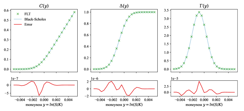
Figure 1: Premium $C(y)$, and Greeks $\Delta(y)$ and $\Gamma(y)$, $S_{0}=100$, $r=6\%$ , $\sigma=1\%$, and $T=5$ days.

For the case where only one dividend $D$ is paid is paid at time $t$ for an option expiring in $T=1$ year and the market conditions are $S_{0}=100$, $r=6\%$, $\sigma=30\%$, table 1 compares the values of the FLT pricer with the Thakoor and Bhuruth (2018) European pricer (TB) for dividends paid very close to the reference date ($t=0.0001$), $6$ months ($t=0.5$) and very close to expiry ($t=0.9999$) for in-the-money, at-the-money, and out-off-the-money strikes $K=70$, $K=100$, and $K=130$ respectively. The prices from the FLT pricer agree with the ones from TB pricer. The FLT was discretized with $N=1024$ equally spaced points, and TB uses $N=500$ integration points with $\xi=6.5$ standard deviations. Both prices have the final strike adjusted to account for the dividend payment.

Table 1: One dividend payment - Comparison with Thakoor, and Bhuruth model.

		$K=70$			$K=100$			$K=130$
t	D	FLT	TB	Diff.	FLT	TB	Diff.	FLT	TB	Diff.
0.0001	7	$34.3193$	$34.3193$	2.76e-12	$13.6870$	$13.6870$	9.63e-13	$4.1862$	$4.1862$	3.19e-13
0.5000	7	$34.6419$	$34.6419$	3.55 e-14	$14.2172$	$14.2172$	1.42e-13	$4.5808$	$4.5808$	3.11e-14
0.9999	7	$34.9844$	$34.9844$	2.55 e-08	$14.7170$	$14.7170$	2.39e-08	$4.9195$	$4.9195$	2.32e-08
0.0001	20	$33.1952$	$33.1952$	4.76 e-13	$11.7740$	$11.7740$	3.45e-13	$2.9221$	$2.9221$	3.46e-14
0.5000	20	$34.0504$	$34.0504$	3.55 e-14	$13.3326$	$13.3326$	1.49e-13	$4.0013$	$4.0013$	2.13e-14
0.9999	20	$34.9842$	$34.9842$	2.55 e-08	$14.7168$	$14.7168$	2.44e-08	$4.9194$	$4.9194$	2.32e-08
0.0001	50	$31.1664$	$31.1664$	2.38 e-13	$7.3596$	$7.3596$	1.10e-13	$0.7210$	$0.7210$	2.44e-15
0.5000	50	$32.9077$	$32.9077$	1.84e-06	$11.5707$	$11.5707$	5.51e-14	$2.9205$	$2.9205$	4.13e-14
0.9999	50	$34.9840$	$34.9840$	2.55e-08	$14.7165$	$14.7165$	2.44e-08	$4.9192$	$4.9192$	2.32e-08

Starting from the same market conditions and strikes used in table (1), table (2) adds two cases with multiple dividends and compares the Greeks from the FLT pricer, namely $\Delta$, and $\Gamma$, against Greeks from a numeric bump in the stock price of $h=0.01$, so that:

$$\Delta_{n} =\frac{\mathrm{FLT}(S+h)-\mathrm{FLT}(S-h)}{2h},$$ (4.1)

$$\Gamma_{n} =\frac{\Delta(S+h)-\Delta(S-h)}{2h}.$$ (4.2)

For these simulations, the FLT uses $N=100$ equally spaced points. It can be seen that the numerical Greeks agree with the ones from the numeric bump central derivative.

Table 2: Greeks - Analytical and numerical bumps.

	$(t_{i},D_{i})=\{(0.2,4),(0.4,5),(0.6,6),(0.8,3)\}$					$(t_{i},D_{i})=\{(0.2,9),(0.6,9)\}$
K	FLT	$10^{2}\Delta$	$10^{2}\Delta_{n}$	$10^{4}\Gamma$	$10^{4}\Gamma_{n}$	FLT	$10^{2}\Delta$	$10^{2}\Delta_{n}$	$10^{4}\Gamma$	$10^{4}\Gamma_{n}$
70	$34.1131$	$95.41$	$95.41$	$35.99$	$35.99$	$33.9703$	$95.69$	$95.69$	$34.83$	$34.83$
100	$13.4083$	$63.41$	$63.41$	$137.87$	$137.87$	$13.1728$	$63.41$	$63.41$	$140.34$	$140.34$
130	$4.0395$	$27.40$	$27.40$	$120.74$	$120.74$	$3.8780$	$26.91$	$26.91$	$121.80$	$121.80$

Concerning performance, when compared to the TB pricer, the FLT pricer presents better results because it reaches the same level of accuracy faster and has the advantage of also delivering the Greeks $\Delta$, $\Gamma$, and $\Theta$ together with the option’s premium. Figure 2 shows some simulations for time versus accuracy. The line (a) shows the four dividend case $(t_{i},D_{i})=\{(0.2,4),(0.4,5),(0.6,6),(0.8,3)\}$ and the line (b) shows the two dividend case $(t_{i},D_{i})=\{(0.2,9),(0.6,9)\}$. The columns show strikes $70,100,$ and $130$. To estimate a true value both prices were simulated with extreme discretizations finding prices $\hat{p}_{a}$ and $\hat{p}_{b}$ which agree with each other with an error of order (1.0E-11) for the case (a) and order (1.0E-14) for the case (b). The accuracy is measured by:

$$\text{Accuracy}_{i} =-\log\left(|p_{i}-\hat{p}|\right),$$ (4.3)

for each simulation. The time taken is measured by running 10 batches of 25 evaluations, and selecting the best average time, therefore, if the batch took time $b_{j}$ for $(j\in 1,\dots,10)$, $t_{i}$ is:

$$t_{i}=\frac{\min\{b_{j}\}}{25}.$$ (4.5)

To give a sense of variance of the time measured, the size $s_{i}$ of each marker in figure 2 is proportional to:

$$s_{i}=\frac{\min\{b_{j}\}}{\max\{b_{j}\}}$$ (4.6)

thus simulations with greater variance have smaller markers. Everything was run on a PC with 16GB of RAM, an intel i7 processor with 2.60GHz, 6 cores, the L1, L2, and L3 cache sizes are 384KB, 1.5MB, and 12MB respectively.

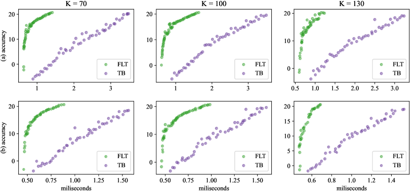
Figure 2: Time and Accuracy comparison. (a) $(t_{i},D_{i})=\{(0.2,4),(0.4,5),(0.6,6),(0.8,3)\}$. (b) $(t_{i},D_{i})=\{(0.2,9),(0.6,9)\}$.

5 Conclusion

This work has presented a numerical procedure able to price and hedge options with discrete multiple dividends using the fast Laplace transform. The FLT is a great tool for solving differential equations and delivers great performance and stability when applied to options pricing with constant volatility. Brazilian listed equity options represent a significant¢ market and are a perfect fit for this approach, but other markets can also benefit from this methodology.

Appendix A Proofs of theorems and corollaries

Proof 1 (Theorem 1).

Let $\pi_{t}$ be a self-financing portfolio of a long position in a security $V_{t}$, a short position on the stock price $S_{t}$, and a cash account to invest the received dividends up to time $t$: $I_{t}$. The value of this portfolio at any time is given by:

$$\pi_{t}=V_{t}-\Delta_{t}(S_{t}+I_{t}).$$ (A.1)

The derivative of this portfolio is given by:

$$\mathrm{d}\pi_{t} =\frac{\partial V_{t}}{\partial t}\mathrm{d}t+\frac{\partial V_{t}}{\partial S_{t}}\mathrm{d}S_{t}+\frac{\mathrm{d}\left\langle S_{t},S_{t}\right\rangle}{2}\frac{\partial^{2}V_{t}}{\partial S_{t}^{2}}+\mathcal{J}V_{t}-\Delta_{t}(\mathrm{d}S_{t}+\mathrm{d}I_{t})$$ (A.2)

Assuming that the security value is continuous for all $t\in[0,T]$, we have $\mathcal{J}V_{t}=V_{t}(S_{t})-V_{t^{-}}(S_{t^{-}})=0,\,\forall t\in[0,T]$, additionally with equations (2.1) and (2.3) follows that:

$$\mathrm{d}\pi_{t} =\frac{\partial V_{t}}{\partial t}\mathrm{d}t+\frac{\partial V_{t}}{\partial S_{t}}(S_{t}r_{t}\mathrm{d}t+S_{t}\sigma_{t}\mathrm{d}W_{t})+\frac{(\sigma_{t}S_{t})^{2}}{2}\frac{\partial^{2}V_{t}}{\partial S_{t}^{2}}\mathrm{d}t-\Delta_{t}\left((S_{t}+I_{t})r_{t}\mathrm{d}t+S_{t}\sigma_{t}\mathrm{d}W_{t}\right),$$ (A.3)

choosing $\Delta_{t}=\frac{\partial V_{t}}{\partial S_{t}}$ we hedge the risk $dW_{t}$ away, turning $\pi_{t}$ into a risk free portfolio hence $d\pi_{t}=\pi_{t}r_{t}dt$. Moreover:

$$\pi_{t}r_{t}\mathrm{d}t =\frac{\partial V_{t}}{\partial t}\mathrm{d}t+\frac{(\sigma_{t}S_{t})^{2}}{2}\frac{\partial^{2}V_{t}}{\partial S_{t}^{2}}\mathrm{d}t-\Delta_{t}I_{t}r_{t}\mathrm{d}t,$$ (A.4)

$$(V_{t}-\Delta_{t}(S_{t}+I_{t}))r_{t} =\frac{\partial V_{t}}{\partial t}+\frac{(\sigma_{t}S_{t})^{2}}{2}\frac{\partial^{2}V_{t}}{\partial S_{t}^{2}}-\Delta_{t}I_{t}r_{t},$$ (A.5)

$$0 =\frac{\partial V_{t}}{\partial t}+\frac{(\sigma_{t}S_{t})^{2}}{2}\frac{\partial^{2}V_{t}}{\partial S_{t}^{2}}+S_{t}r_{t}\frac{\partial V_{t}}{\partial S_{t}}-r_{t}V_{t}.$$ (A.6)

∎

Proof 2 (Corollary 1).

Taking the derivative of $X_{t}=e^{-\int_{0}^{t}r_{u}\;\mathrm{d}u}V_{t}$ we get:

$$\mathrm{d}X_{t} =-r_{t}e^{-\int_{0}^{t}r_{u}\;\mathrm{d}u}V_{t}\mathrm{d}t+e^{-\int_{0}^{t}r_{u}\;\mathrm{d}u}\mathrm{d}V_{t}$$

$$=e^{-\int_{0}^{t}r_{u}\;\mathrm{d}u}\left(-rV_{t}\mathrm{d}t+\frac{\partial V_{t}}{\partial t}\mathrm{d}t+\frac{1}{2}(\sigma_{t}S_{t})^{2}\frac{\partial^{2}V_{t}}{\partial S_{t}^{2}}\mathrm{d}t+\frac{\partial V_{t}}{\partial S_{t}}(S_{t}r_{t}\mathrm{d}t+S_{t}\sigma_{t}\mathrm{d}W_{t})\right),$$ (A.7)

from theorem 1 we know that the terms multiplying $dt$ add to zero, thus:

$$\mathrm{d}X_{t} =e^{-\int_{0}^{t}r_{u}\;\mathrm{d}u}\frac{\partial V_{t}}{\partial S_{t}}S_{t}\sigma_{t}\mathrm{d}W_{t}$$

$$=S_{t}\sigma_{t}\frac{\partial X_{t}}{\partial S_{t}}\mathrm{d}W_{t},$$ (A.8)

proving that $X_{t}$ is a martingale. ∎

Proof 3 (Theorem 2).

At any time $t$ the option holder can decide between exercising the option, hence receiving its intrinsic value $g_{i}(S_{t})$ or keeping the option. Therefore, the value of the American option at any time $t$ can be described as:

$$C_{t}=\max\left\{\mathbb{E}\left[\left.e^{-\int_{t}^{u}r_{v}\;\mathrm{d}v}C_{u>t}\right|\mathcal{F}_{t}\right],g_{n}(S_{t})\right\},$$ (A.9)

where $t<u<=T$. To prove that it is never optimal to exercise, it suffices to prove that for each $t\in[t_{i},t_{i+1})$:

$$\mathbb{E}\left[\left.e^{-\int_{t}^{t_{i+1}}r_{v}\;\mathrm{d}v}C_{t_{i+1}}\right|\mathcal{F}_{t}\right]\geq g_{i}(S_{t}).$$ (A.10)

Let’s prove it by backward induction. Starting with the last period where $t\in[t_{n},T]$, we have:

$$\mathbb{E}\left[\left.e^{-\int_{t}^{T}r_{v}\;\mathrm{d}v}g_{n}(S_{T})\right|\mathcal{F}_{t}\right] \geq\mathbb{E}\left[\left.g_{n}\left(e^{-\int_{t}^{T}r_{v}\;\mathrm{d}v}S_{T}\right)\right|\mathcal{F}_{t}\right]\text{ (lemma \ref{lemma:call_payof_convex}),}$$

$$\geq g_{n}\left(\mathbb{E}\left[\left.e^{-\int_{t}^{T}r_{v}\;\mathrm{d}v}S_{T}\right|\mathcal{F}_{t}\right]\right)\text{ (Jensen's inequality),}$$

$$=g_{n}\left(S_{t}\right)\text{ (martingale property).}$$ (A.11)

Now, let’s take an instantaneous step back in time for the exact moment when the last dividend goes ex-date, then:

$$C_{t_{n}^{-}} =max\left\{C_{t_{n}},g_{n-1}(S_{t_{n}^{-}})\right\}$$

$$=max\left\{C_{t_{n}},g_{n}(S_{t_{n}})\right\}\text{ (equation \eqref{eq:call_payof_continuous})},$$

$$\therefore\,C_{t_{n}^{-}} =C_{t_{n}}\text{ (by equation \eqref{eq:last_dividend_call_intrinsic})}.$$ (A.12)

To complete the inductive argument, consider a time $t\in[t_{k},t_{k+1})$, our inductive hypothesis is:

$$C_{t_{k+1}^{-}} \geq g_{k}(S_{t_{k+1}^{-}}),$$ (A.13)

from here we can proceed in the same manner as we did deriving equation (A.11):

$$\mathbb{E}\left[\left.e^{-\int_{t}^{t_{k+1}}r_{u}\;\mathrm{d}u}C_{t_{k+1}^{-}}\right|\mathcal{F}_{t}\right] \geq\mathbb{E}\left[\left.e^{-\int_{t}^{t_{k+1}}r_{u}\;\mathrm{d}u}g_{k}(S_{t_{k+1}^{-}})\right|\mathcal{F}_{t}\right]$$

$$\geq\mathbb{E}\left[\left.g_{k}\left(e^{-\int_{t}^{t_{k+1}}r_{u}\;\mathrm{d}u}S_{t_{k+1}^{-}}\right)\right|\mathcal{F}_{t}\right]$$

$$\geq g_{k}\left(\mathbb{E}\left[\left.e^{-\int_{t}^{t_{k+1}}r_{u}\;\mathrm{d}u}S_{t_{k+1}^{-}}\right|\mathcal{F}_{t}\right]\right)$$

$$=g_{k}\left(S_{t}\right),$$ (A.14)

which proves the induction. ∎

Lemma 1.

For any $g(x)=\max\left\{x-K,0\right\}$, $x,K>0$ we have:

$$g(ax)\leq ag(x),$$ (A.15)

when $a\in[0,1]$. The proof is a direct application of Jensen’s inequality to the convex function $g(x)$.

Proof 4 (Theorem 3).

Fist, note that the process $X_{t}=e^{-\int_{0}^{t}r_{u}\;\mathrm{d}u}(S_{t}+I_{t})$ is a martingale:

$$\mathrm{d}X_{t} =-r_{t}X_{t}\mathrm{d}t+e^{-\int_{0}^{t}r_{u}\;\mathrm{d}u}(\mathrm{d}S_{t}+\mathrm{d}I_{t})$$

$$=-r_{t}X_{t}\mathrm{d}t+e^{-\int_{0}^{t}r_{u}\;\mathrm{d}u}(r_{t}S_{t}\mathrm{d}t+\sigma_{t}S_{t}\mathrm{d}W_{t}+\mathcal{J}S_{t}+rI_{t}\mathrm{d}t+\mathcal{J}I_{t}),$$

$$=-r_{t}X_{t}\mathrm{d}t+e^{-\int_{0}^{t}r_{u}\;\mathrm{d}u}(r_{t}S_{t}\mathrm{d}t+\sigma_{t}S_{t}\mathrm{d}W_{t}+rI_{t}\mathrm{d}t)\text{, because }(\mathcal{J}S_{t}=-\mathcal{J}I_{t}),$$

$$=-r_{t}X_{t}\mathrm{d}t++r_{t}X_{t}\mathrm{d}t+e^{-\int_{0}^{t}r_{u}\;\mathrm{d}u}\sigma_{t}S_{t}\mathrm{d}W_{t},$$

$$=e^{-\int_{0}^{t}r_{u}\;\mathrm{d}u}\sigma_{t}S_{t}\mathrm{d}W_{t}.$$ (A.16)

Therefore:

$$\mathbb{E}\left[\left.e^{-\int_{0}^{T}r_{u}\;\mathrm{d}u}(S_{T}+I_{T})\right|\mathcal{F}_{t}\right]=e^{-\int_{0}^{t}r_{u}\;\mathrm{d}u}(S_{t}+I_{t}),$$

$$\mathbb{E}\left[\left.S_{T}\right|\mathcal{F}_{t}\right]=e^{\int_{t}^{T}r_{u}\;\mathrm{d}u}(S_{t}+I_{t})-I_{T}.$$ (A.17)

∎

Proof 5 (Theorem 4).

Letting $x(n)=\rho n+x_{0}$ and taking the continuous derivative of $f(x)u(x-x_{0})$ with respect to $x$:

$$[f(x)u(x-x_{0})]^{\prime} =f^{\prime}(x)u(x-x_{0})+f(x)\delta(x-x_{0})\implies$$ (A.18)

$$\frac{\mathrm{d}[f(n)u(n)]}{\mathrm{d}n}\frac{\mathrm{d}n}{\mathrm{d}x} =\frac{\mathrm{d}f(x)}{\mathrm{d}x}u(n)+f(n)\mathbf{1}_{n=0},$$ (A.19)

then applying the discrete Laplace transform to both sides:

$$\sum_{n=0}^{N-1}e^{-s_{k}n}\frac{\mathrm{d}[f(n)u(n)]}{\mathrm{d}n}\frac{\mathrm{d}n}{\mathrm{d}x} =\sum_{n=0}^{N-1}e^{-s_{k}n}\frac{\mathrm{d}f(x)}{\mathrm{d}x}u(n)+\sum_{n=0}^{N-1}e^{-s_{k}n}f(n)\mathbf{1}_{n=0},$$

$$=\sum_{n=0}^{N-1}e^{-s_{k}n}\frac{\mathrm{d}f(x)}{\mathrm{d}x}+f_{0},$$ (A.20)

The left-hand side of equation (5) can be written with the inverse Laplace transform:

$$\sum_{n=0}^{N-1}e^{-s_{k}n}\frac{\mathrm{d}[f(n)u(n)]}{\mathrm{d}n}\frac{\mathrm{d}n}{\mathrm{d}x} =\sum_{n=0}^{N-1}e^{-s_{k}n}\frac{\mathrm{d}\left(\frac{1}{N}\sum_{l=0}^{N-1}e^{s_{l}n}\bar{f}_{l}\right)}{\mathrm{d}n}\frac{1}{\rho}=\sum_{n=0}^{N-1}e^{-s_{k}n}\left(\frac{1}{N}\sum_{l=0}^{N-1}e^{s_{l}n}s_{l}\bar{f}_{l}\right)\frac{1}{\rho}$$

$$=\frac{1}{N\rho}\sum_{n=0}^{N-1}\sum_{l=0}^{N-1}e^{(s_{l}-s_{k})n}s_{l}\bar{f}_{l}=\frac{1}{N\rho}\sum_{l=0}^{N-1}s_{l}\bar{f}_{l}\sum_{n=0}^{N-1}e^{\frac{i2\pi(l-k)n}{N}}$$

$$=\frac{1}{N\rho}\sum_{l=0}^{N-1}s_{l}\bar{f}_{l}N\mathbf{1}_{l=k}=\frac{s_{k}}{\rho}\bar{f}_{k}.$$ (A.21)

Taking sequences from $k\in\{0,\dots,N-1\}$ and rewriting equation (5) in terms of the discrete Laplace transform finishes the proof:

$$\frac{\{s\}_{N}}{\rho}\mathcal{L}_{d}\{f\}_{N} =\mathcal{L}_{d}\{f^{\prime}(x)\}_{N}+f_{0},$$

$$\therefore\mathcal{L}_{d}\{f^{\prime}(x)\}_{N} =\frac{\{s\}_{N}}{\rho}\mathcal{L}_{d}\{f\}_{N}-f_{0}.$$ (A.22)

∎

References

• Black and Scholes (1973) Black, F., Scholes, M., 1973. The pricing of options and corporate liabilities. Journal of Political Economy 81, 637–654.
• Brunton (2020) Brunton, S., 2020. The laplace transform: A generalized fourier transform. URL: https://www.youtube.com/watch?v=7UvtU75NXTg. accessed: 2022-09-16.
• Brunton and Kutz (2022) Brunton, S.L., Kutz, J.N., 2022. Data-driven science and engineering: Machine learning, dynamical systems, and control. Cambridge University Press.
• Cooley and Tukey (1965) Cooley, J.W., Tukey, J.W., 1965. An algorithm for the machine calculation of complex fourier series. Mathematics of computation 19, 297–301.
• Haug (2007) Haug, E., 2007. The Complete Guide to Option Pricing Formulas. McGraw-Hill Education. URL: https://books.google.com.br/books?id=tuoJAQAAMAAJ.
• Haug et al. (2003) Haug, E.G., Haug, J., Lewis, A., 2003. Back to basics: a new approach to the discrete dividend problem .
• Merton (1973) Merton, R.C., 1973. Theory of rational option pricing. The Bell Journal of Economics and Management Science 4, 141–183. URL: http://www.jstor.org/stable/3003143.
• Thakoor and Bhuruth (2018) Thakoor, D., Bhuruth, M., 2018. Fast quadrature methods for options with discrete dividends. Journal of Computational and Applied Mathematics 330, 1–14. URL: https://www.sciencedirect.com/science/article/pii/S0377042717303953, doi:https://doi.org/10.1016/j.cam.2017.08.006.