Wigner Distribution Deconvolution Adaptation for Live Ptychography Reconstruction

Abstract

We propose a modification of Wigner Distribution Deconvolution (WDD) to support live processing ptychography. Live processing allows to reconstruct and display the specimen transfer function gradually while diffraction patterns are acquired. For this purpose we reformulate WDD and apply a dimensionality reduction technique that reduces memory consumption and increases processing speed. We show numerically that this approach maintains the reconstruction quality of specimen transfer functions as well as reduces computational complexity during acquisition processes. Although we only present the reconstruction for Scanning Transmission Electron Microscopy (STEM) datasets, in general, the live processing algorithm we present in this paper can be applied to real-time ptychographic reconstruction for different fields of application.

1 Introduction

Four-dimensional STEM is an experimental modality where a wide range of computational methods can extract information on the specimen and reduce the acquired data for human interaction (Ophus, 2019). The acquisition schema of four-dimensional STEM is shown in Figure 1. Acquiring such comprehensive data and applying computational analysis and reconstruction workflows allows observation of material properties by electron microscopy that are not accessible with simple detectors and signal processing methods (Ophus, 2019). Since it generates large amounts of data (Spurgeon et al., 2021), making algorithms and implementations efficient in their use of computer memory and processing time requires special attention.

If a computational method to process the recorded data is only implemented for offline use, microscopists have to acquire data relying only on simple contrast methods or even without any feedback at all. An implementation for live processing, in contrast, allows interactive use of the microscope based on advanced computational contrast mechanisms, monitoring the acquisition process, evaluating data quality, or automatically controlling the instrument in a closed loop. This requires suitable interfaces to the microscope to receive a live data stream as well as implementations that are capable to process data gradually while they arrive (Nord et al., 2020).

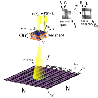
Figure 1: Four-dimensional STEM acquisition for a scanning point $s\in[S]$ with definition of real space grid $\mathbf{r}=(r_{y},r_{x})\in\mathbb{R}^{2}$, reciprocal space grid $\mathbf{q}=(q_{y},q_{x})\in\mathbb{R}^{2}$, scanning grid $\hat{\mathbf{r}}=(\hat{r}_{y},\hat{r}_{x})\in\mathbb{R}^{2}$ and spatial frequency grid $\hat{\mathbf{q}}=(\hat{q}_{y},\hat{q}_{x})\in\mathbb{R}^{2}$.

Ptychography (Hoppe, 1969a; Hoppe & Strube, 1969; Hoppe, 1969b) can be used to extract a quantitative object transfer function for a specimen using 4D STEM data. It takes advantage of information from local overlap of the illuminated regions. Recent years have seen a widespread increase in the development of ptychography algorithms by different approaches, such as inspired by the classical alternating projection method, i.e., PIE reconstruction algorithm (Rodenburg & Faulkner, 2004; Maiden & Rodenburg, 2009), other optimization-based approaches (Bostan et al., 2018; Wen et al., 2012), as well as direct methods. Single Side Band (SSB) (Rodenburg et al., 1993; Pennycook et al., 2015; Yang et al., 2015) and WDD (Rodenburg & Bates, 1992; Li et al., 2014; Yang et al., 2016) are examples of direct ptychography methods that extract the relevant information in a sequential processing flow, as opposed to iterative methods that optimize the object transfer function in a loop over the input data.

With SSB as an example, Strauch et al. (Strauch et al., 2021b) showed previously that direct, linear methods are particularly suitable for live processing since the result can always be expressed as the sum of partial results from processing subsets of the input data. However, reconstruction with SSB relies on the weak phase object approximation. Compared to SSB, WDD does not have this limitation (Yang et al., 2017). At the same time, the data reduction in WDD is a linear function of the input data like in SSB, meaning it is a good candidate for live ptychography. Strong binning is used as dimensionality reduction method in (Pelz et al., 2021) to reduce the processing time for SSB after an acquisition is completed.

1.1 Related Works

A real-time phase reconstruction approach based on integrated Center of Mass (COM) is proposed in (Yu et al., 2021). That method does not require storing the entire four-dimensional dataset in memory and reconstructs the phase from strongly reduced COM information instead of full diffraction patterns. The COM can be computed efficiently from diffraction data so that this algorithm can reconstruct large-scale data. The authors coined the real-time approach as riCOM.

1.2 Summary of Contributions

Here we demonstrate live reconstruction using the eigenfunctions of a harmonic oscillator instead of binning as a base for dimensionality reduction. In addition to data reduction, this transformation can replace the Fourier transform in several steps of the WDD method while retaining a reconstruction that is very similar to a result without dimensionality reduction. Furthermore, by building on the matrix representation of the discrete Fourier transform, we can process the intensity data and reconstruct the specimen transfer function gradually from subsets of the input data in a streaming fashion. As a benchmark, we compare the result of Live WDD with the implementation of WDD in PyPtychoSTEM (Pennycook & Hofer, 2021) as well as Live SSB (Strauch et al., 2021b).

The codes used and to reproduce the result in this paper are available at the URL below:

https://github.com/Ptychography-4-0/LiveWDD

1.3 Notations

We provide notations used throughout this article. Vectors are written in bold small-cap letters $\mathbf{x}\in\mathbb{C}^{L}$ and matrices are written as a bold big-cap letter $\mathbf{A}\in\mathbb{C}^{K\times L}$ for a complex field $\mathbb{C}$ and for a real field $\mathbb{R}$. A matrix can also be written by indexing its elements

$$\mathbf{A}=\left(a_{k\ell}\right),\quad\text{where}\quad k\in[K],\ell\in[L].$$

The set of integers is written as $[N]:=\{1,2,\ldots,N\}$ and calligraphic letters are used to define functions $\mathcal{A}:\mathbb{C}\rightarrow\mathbb{C}$. Specifically, we denote the discrete two-dimensional Fourier transform by $\mathcal{F}$. For both matrices and vectors, the notation $\circ$ is used to represent an element-wise product, also called Hadamard product. $\mathbf{A}^{T}$ is used to denote the transpose of a matrix $\mathbf{A}$. The notation $\text{vec}:\mathbb{C}^{N\times N}\rightarrow\mathbb{C}^{N^{2}}$ is an operator that vectorizes a matrix, and $\text{mat}:\mathbb{C}^{N^{2}}\rightarrow\mathbb{C}^{N\times N}$ constructs a matrix from a vector. The complex conjugate is indicated by a bar. For a matrix $\overline{\mathbf{X}}$, it is the element-wise conjugate. The convolution and Kronecker operator are denoted by $\circledast$ and $\otimes$, respectively. The partial derivative is given by $\partial$, and $\nabla$ is the nabla or vector differential operator.

2 Wigner Distribution Deconvolution

In this section, we introduce the matrix representation of the WDD method developed from its original formulation as in (Rodenburg & Bates, 1992) and an Open Source implementation from (Pennycook & Hofer, 2021). In order to visualize the definition for different spaces used in this article we refer to Figure 1. The specimen transfer function is denoted by a matrix $\mathbf{O}\in\mathbb{C}^{N\times N}$ where values at the row and column indices $(i,j)$ define the object function at a position $\mathbf{r}\in[N^{2}]$ in the specimen plane. Similarly, values of the illuminating probe $p(\mathbf{r})$ in the specimen plane at position $\mathbf{r}$ without shifting can be written in matrix form as $\mathbf{P}\in\mathbb{C}^{N\times N}$.

For all shifting coordinates in the set of flattened scan position coordinates, $\hat{\mathbf{r}_{s}}\in\{\hat{\mathbf{r}}_{1},\hat{\mathbf{r}}_{2},\dots,\hat{\mathbf{r}}_{S}\}$, we write the shifted matrix probe as $\mathbf{P}_{s}$ for $s\in[S]$, where the $S=S_{y}\times S_{x}$ is the set of scanning points. Consequently, the matrix for a shifted matrix probe is given by

$$\left(p_{ij}\right)_{s}=p(\mathbf{r}-\hat{\mathbf{r}}_{s}),\quad\text{where}\quad i,j\in[N],$$

Here we define the object, probe, diffraction patterns and the scanning points on equi-spaced rectangular grids. Hence, the usual implementation of the discrete Fourier transform can be used. The intensity of the diffraction pattern at each scanning point can be written as

$$\mathbf{I}_{s}=\left|\mathcal{F}_{\mathbf{r}}\left(\mathbf{P}_{s}\circ\mathbf{O}\right)\right|^{2}\quad\text{for}\quad s\in[S].$$ (1)

Similar to the real space coordinate, each pattern $\mathbf{I}_{s}$ for scan position $s$ is indexed by flattened reciprocal space coordinates $\mathbf{q}_{s}\in\{\mathbf{q}_{1},\mathbf{q}_{2},\dots,\mathbf{q}_{N^{2}}\}$, where $N^{2}$ denotes the pair index in the two-dimensional grid in reciprocal space. It should be noted that the complete set of diffraction patterns can be written as flattened scanning points index $\mathbf{I}\in\mathbb{R}^{S\times N\times N}$ or as a four-dimensional tensor $\mathbf{I}\in\mathbb{R}^{S_{y}\times S_{x}\times N\times N}$ indexed by the two-dimensional scan position $\hat{\mathbf{r}}$ and the two-dimensional reciprocal space coordinate $\mathbf{q}$, corresponding to the diffraction angle.

The two-dimensional Fourier transform with respect to the object and probe grid coordinates $\mathbf{r}$ is written as $\mathcal{F}_{\mathbf{r}}$, with respect to the scan coordinate $\hat{\mathbf{r}}$ as $\mathcal{F}_{\hat{\mathbf{r}}}$, and the inverse transforms consequently as $\mathcal{F}_{\mathbf{q}}^{-1}$ and $\mathcal{F}_{\hat{{\mathbf{q}}}}^{-1}$. The WDD algorithm estimates the object from the intensity of diffraction patterns and an estimate of the probe. Picking up from (Rodenburg & Bates, 1992, eq.8) where a relation between the object’s and probe’s Wigner distributions $\mathbf{W}_{O}\in\mathbb{C}^{S_{y}\times S_{x}\times N\times N}$ resp. $\mathbf{W}_{P}\in\mathbb{C}^{S_{y}\times S_{x}\times N\times N}$ is shown:

$$\mathbf{W}_{O}=\frac{\mathcal{F}_{\mathbf{{q}}}^{-1}\left(\mathcal{F}_{\hat{{\mathbf{r}}}}\left(\mathbf{I}\right)\right)\overline{\mathbf{W}_{P}}}{\left|\mathbf{W}_{P}\right|^{2}+\epsilon}$$ (2)

with $\mathbf{W}^{v}_{P}=\mathcal{F}_{\mathbf{q}}^{-1}\left(\mathcal{F}_{\mathbf{r}}\left(\mathbf{P}\right)\overline{\mathcal{F}_{\mathbf{r}}\left(\mathbf{P}\right)}\big{|}_{\left(\mathbf{q}+\hat{\mathbf{q}}_{v}\right)}\right)$, where $\mathcal{F}_{\mathbf{r}}\left(\mathbf{P}\right)\big{|}_{\left(\mathbf{q}+\hat{\mathbf{q}}_{v}\right)}$ denotes a shift in reciprocal space of the Fourier-transformed probe for specific index $v$.

By inserting an estimate of the probe $\mathbf{\widetilde{P}}$ and calculating the probe’s Wigner distribution $\mathbf{\widetilde{W}}_{P}$, one can estimate the object’s Wigner distribution $\mathbf{\widetilde{W}}_{O}$. Following (Rodenburg & Bates, 1992), an estimate for the object $\mathbf{\widetilde{O}}$ can be obtained from $\mathbf{\widetilde{W}}_{O}$ as

$$\mathbf{\widetilde{O}}=\frac{\mathcal{F}_{\hat{\mathbf{q}}}^{-1}\left(\mathcal{F}_{\mathbf{r}}\left(\mathbf{\widetilde{W}}_{O}\right)\bigg{|}_{\left(\mathbf{q}=0\right)}\right)}{\sqrt{\mathcal{F}_{\mathbf{r}}\left(\mathbf{\widetilde{W}}_{O}\right)\bigg{|}_{\left(\hat{\mathbf{q}}=0,\mathbf{q}=0\right)}}}\in\mathbb{C}^{S_{y}\times S_{x}},$$ (3)

with $\mathbf{q}=0$ and $\left(\hat{\mathbf{q}}=0,\mathbf{q}=0\right)$ denoting extraction of a subset at the specified coordinates.

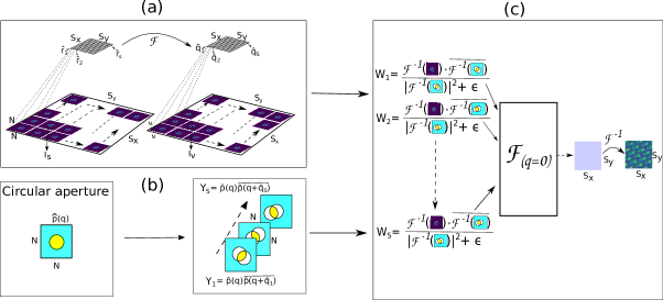
Figure 2: The schematic diagram for classical WDD. (a). The calculation of spatial frequencies $\hat{\mathbf{q}}_{v}$ of a four-dimensional STEM diffraction pattern dataset is given by applying two-dimensional Fourier transform in the real space scan coordinate $\hat{\mathbf{r}}_{s}$, (b). For each spatial frequency the autocorrelation of the circular aperture is calculated, i.e., initial probe in reciprocal space, (c). Apply a two-dimensional inverse Fourier transform for each diffraction pattern dataset on each spatial frequency and the probe autocorrelation and use it for the deconvolution process by using a Wiener filter. Afterward, apply Fourier transform and extract for reciprocal space $\mathbf{q}=0$ to get an image on spatial frequency before estimating the object in real space scan coordinate with a two-dimensional inverse Fourier transform.

A visualization of the WDD algorithm is depicted in Figure 2.

Calculating the deconvolution in (2) may consume large amounts of memory for typical four-dimensional STEM data if implemented naively following the equations above since a Fourier transform of the original data, as well as $\mathbf{W}_{P}$, which has the same size as the input data, might be instantiated at the same time. Furthermore, they are complex-valued and may require higher numerical precision than the input data. Additionally, this algorithm works on entire datasets, preventing a direct implementation of live processing.

To address the computational complexity and allow live processing we introduce a dimensionality reduction to reduce the size of the input data and $\mathbf{W}_{P}$, and rearrange the WDD algorithm. The modification allows us to process the intensity data sequentially and update the reconstruction as the scan proceeds to acquire new intensity data.

3 Validation

Since ptychography is a quantitative reconstruction technique, any implementation should demonstrate that it is correct, i.e., that it reconstructs arbitrary object functions and/or illuminations quantitatively within its inherent limitations. Simulated datasets of a crystalline specimen resemble the real-world data that ptychography is used on in electron microscopy, but they often have very high symmetry and have no natural orientation. That means errors such as a rolled, phase-reversed or inverted reconstruction, or multiplication with a factor may not be obvious. Such errors can, for example, be caused by mixing Fourier transform and inverse Fourier transform, by adding or omitting a complex conjugation, or by incorrect use of FFT shift resp. inverse FFT shift. For this reason the implementations used in this paper were validated with a simple procedurally generated asymmetric test image. It is clearly recognizable starting at $25\times 25$ px and contains a wrapped phase ramp at an odd angle that creates a characteristic single spot in the Fourier transform, allowing to visually confirm the correct relation between real and reciprocal space.

A test dataset was created from this test object using multiplication with a synthetic illumination rolled to the scan position, inverse FFT shift, Fourier transform and FFT shift. The illumination was calculated from a synthetic circular aperture with value 17 to catch scaling issues that may not be apparent if the value 1 was used. The illumination function in amplitude and phase as well as the calculated amplitude, phase and intensity from the forward simulation were visually inspected to conform with the expected values. In particular, the simulated diffraction patterns contain a shifted replica of the illuminating aperture at the expected position as a signature of the wrapped phase ramp. A virtual bright field image of the simulated dataset confirmed the correct spatial arrangement of the diffraction patterns. See Figure 4 for a sample diffraction pattern and a virtual bright field image.

The WDD implementation was then confirmed to reconstruct the object quantitatively in amplitude and phase, taking the band pass filtering of WDD with twice the semiconvergence angle of the aperture into account (Figure 3). The correct scale for the illumination of real-world microscopy data can be derived from a vacuum reference, i.e. a scan with the same parameters but without the specimen. This enables quantitative reconstruction of both amplitude and phase of the object function. A Jupyter notebook with the validation is available at https://github.com/Ptychography-4-0/LiveWDD.

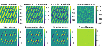
Figure 3: Validation with a procedurally-generated synthetic test dataset: Comparing original object, reconstruction, approximate of the expected result calculated by bandpass-filtering the object with twice the aperture size, and difference between reconstruction and approximate expected value.

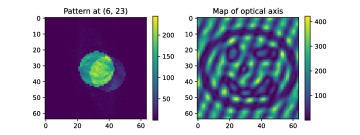
Figure 4: Sample diffraction pattern and projection along the optical axis from the synthetic test dataset that is used for validation.

4 Circular Harmonic Oscillator

In this section we present details of the dimensionality reduction method used.

The rate-limiting step in conventional WDD is the deconvolution of a massive dataset. Therefore, one can improve the performance by projecting the dataset onto a space with lower dimension while retaining the essential information, and performing the resource-intensive steps in this reduced representation. Cropping and binning are simple examples of such projections from higher to lower dimension.

A basis of eigenfunctions of the harmonic oscillator has beneficial properties in this application that are detailed in the following sections. We start first by defining the harmonic oscillator. We provide a brief introduction to this topic and refer the interested readers to the literature (Sakurai, 1994).

4.1 One-Dimensional Harmonic Oscillator

The quantum-mechanical harmonic oscillator (HO) problem is described by the Hamiltonian operator

$$\hat{H}^{[1D]}_{\sigma}=-\frac{\partial_{x}^{2}}{2}+\frac{x^{2}}{2\sigma^{4}}\text{.}$$ (4)

Hartree atomic units are used in this section. Here, $\sigma$ is a length scale parameter that also fixes the scale of the eigenvalues $E^{[1D]}_{n}(\sigma)$ of the operator $\hat{H}^{[1D]}_{\sigma}$, the so called eigenenergies. The eigenvalue problem reads

$$\hat{H}^{[1D]}\psi^{[1D]}_{n}(x)=E^{[1D]}_{n}\psi^{[1D]}_{n}(x)\text{,}\ n\in\mathbb{N}_{0}\text{.}$$ (5)

Then, the energy eigenvalues are

$$E^{[1D]}_{n}(\sigma)=\sigma^{-2}\left(n+\frac{1}{2}\right)$$ (6)

and the corresponding HO eigenfunctions are

$$\psi^{[1D]}_{n}(x)=H_{n}\left(\frac{x}{\sigma}\right)\ \exp\left(-\frac{x^{2}}{2\sigma^{2}}\right)$$ (7)

with the Hermite polynomials $H_{n}$. It can be seen that these eigenfunctions are Hermite polynomials weighted by a Gaussian envelope function. For the usage as a basis, a proper $L_{2}$-normalization is necessary. The normalized Hermite polynomials for several degrees are presented in Figure 5.

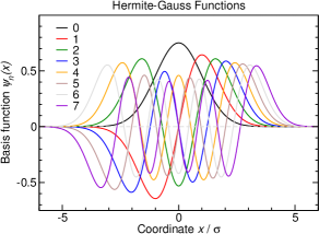
Figure 5: Normalized Hermite-Gauss functions up to $n_{\mathrm{max}}=7$. All functions are either even ($\psi(-x)=\psi(x)$) or odd ($\psi(-x)=-\psi(x)$), depending on the parity of $n$.

4.2 Two-Dimensional Isotropic Harmonic Oscillator

The eigenfunctions of the quantum-mechanical two-dimensional isotropic harmonic oscillator, in the following we will refer to it as circular harmonic oscillator (CHO), can be written as Cartesian product of two HO eigenfunctions. The Hamiltonian

$$\hat{H}^{[2D]}_{\sigma}=-\frac{\IfSubStr{abcdefghijklmnopqrstuvwxyzABCDEFGHIJKLMNOPQRST123456789}{\nabla}{\mathbf{{\nabla}}}{\boldsymbol{{\nabla}}}^{2}}{2}+\frac{\IfSubStr{abcdefghijklmnopqrstuvwxyzABCDEFGHIJKLMNOPQRST123456789}{r}{\mathbf{{r}}}{\boldsymbol{{r}}}^{2}}{2\sigma^{4}}$$ (8)

has the eigenfunctions

$$\psi^{[2D]}_{n_{x}n_{y}}(x,y)=\psi^{[1D]}_{n_{x}}(x/\sigma)\ \psi^{[1D]}_{n_{y}}(y/\sigma)$$ (9)

and the eigenenergies

$$E^{[2D]}_{n_{x}n_{y}}(\sigma)=E^{[1D]}_{n_{x}}(\sigma)+E^{[1D]}_{n_{y}}(\sigma)=\sigma^{-2}\left(n_{x}+n_{y}+1\right)$$ (10)

4.3 Special property of the basis

The HO eigenfunctions with $\sigma=1$ are also eigenfunctions of the Fourier transform (FT) operator, i.e. the Fourier transform of $\psi^{[1D]}_{n}(x)$ is again a Gauss-Hermite function:

$$\mathcal{F}\left(\psi^{[1D]}_{n}(x)\right)=\imath^{n}\psi^{[1D]}_{n}(q),$$ (11)

for $q$ being the reciprocal space coordinate adjoint to $x$. For a non-unity spread, i.e. any $\sigma>0$, the FT produces a spread of $1/\sigma$ in reciprocal space.

Furthermore, transforming a function by this eigenfunction changes a convolution into multiplication similar to a Fourier transform, which is discussed in (Glaeske, 1983, Theorem 4.1). That means transforming into this basis can replace Fourier transforms in the WDD algorithm.

5 Dimensionality Reduction for WDD

The Hermite-Gauss functions defined in (7) can be used as a basis for dimensionality reduction of STEM datasets. We first introduce the matrix notation from sampled Hermite-Gauss function before presenting the procedure to reduce the dimension of the data. Secondly, the transformation will be presented as well as a numerical example for the transformation.

The sampling grid $x$ and scaling factor $\sigma$ in (7) should be adapted so that the basis is centered with respect to the diffraction patterns and scaled to cover the area relevant for WDD, i.e. the area illuminated by the primary beam.

We can construct a matrix from sampled Hermite-Gauss functions as presented below

$$\small\boldsymbol{\psi}_{x}=\begin{pmatrix}\psi^{[1D]}_{n_{1}}(x_{1})\quad\psi^{[1D]}_{n_{2}}(x_{1})&\dots&\psi^{[1D]}_{n_{L}}(x_{1})\\ \psi^{[1D]}_{n_{1}}(x_{2})\quad\psi^{[1D]}_{n_{2}}(x_{2})&\dots&\psi^{[1D]}_{n_{L}}(x_{2})\\ \vdots&\dots&\vdots\\ \psi^{[1D]}_{n_{1}}(x_{N})\quad\psi^{[1D]}_{n_{2}}(x_{N})&\dots&\psi^{[1D]}_{n_{L}}(x_{N})\\ \end{pmatrix}\in\mathbb{R}^{N\times L},$$

where we construct a sampling grid with respect to the center of mass in the $x$ direction. After introducing the matrix representation of the Hermite-Gaussian function, we can define the dimensionality reduction by using this matrix. For a $\mathbf{A}\in\mathbb{R}^{N\times N}$ the projection to the lower dimension using Hermite-Gauss functions can be expressed as

$$\mathcal{H}\left(\mathbf{A}\right):=\boldsymbol{\psi}_{x}^{T}\mathbf{A}^{T}\boldsymbol{\psi}_{y}\in\mathbb{R}^{L\times L}$$ (12)

This function $\mathcal{H}:\mathbb{C}^{N\times N}\rightarrow\mathbb{C}^{L\times L}$ where $L\ll N$ maps from the data with dimension $N\times N$ to a lower dimension $L\times L$.

In contrast to the original two-dimensional discrete Fourier transformation that preserves the dimension of the dataset, this transformation allows flexibility to reduce the dimension. Hence, we can apply this dimensional reduction technique in the deconvolution step in WDD as presented below

$$\mathcal{H}\left(\mathbf{I}_{v}\right) =\mathcal{H}\left(\mathbf{X}_{v}\circledast\mathbf{Y}_{v}\right)\quad\text{for}\quad v\in[S]$$ (13)

$$=\mathcal{H}\left(\mathbf{X}_{v}\right)\mathcal{H}\left(\mathbf{Y}_{v}\right),$$

where now the dimension is reduced from $N\times N$ to $L\times L$ with $L\ll N$. The variable $\mathbf{I}_{v}$ is the intensity of diffraction pattern of specific spatial frequency coordinate $v\in[S]$. Variables $\mathbf{Y}_{v}$ and $\mathbf{X}_{v}$ represent the autocorrelation of the illuminating probe and the autocorrelation of the specimen transfer function, respectively. In parallel with classical WDD, the $\mathcal{H}\left(\mathbf{Y}_{v}\right)$ and $\mathcal{H}\left(\mathbf{X}_{v}\right)$ represent functions at specific spatial frequency $v$ that have similar properties to the Wigner distribution function of the probe and object in conventional WDD.

Transformation to lower dimension can be seen in Figure 6, where we have reduced from dimension $256\times 256$ to $16\times 16$. Since we apply dimensionality reduction to our four-dimensional STEM data, we also have to apply it to the autocorrelation of the illuminating probe to proceed with the deconvolution process, as shown in (13). The transformation from convolution into multiplication by applying the operator $\mathcal{H}$ is derived from the properties of Hermite-Gaussian functions applied to the convolution as introduced in the previous section. Compared to conventional WDD, the deconvolution can be performed in a lower dimension and in a different space with similar properties, and the rest follows similar to WDD.

Figure 6: Dimensionality reduction of PACBED data from SrTiO₃ dataset (Strauch et al., 2021a). (a) PACBED data, (b) Lower Dimension $(16\times 16)$, (c) Reconstructed PACBED

6 Live Processing WDD

A conventional WDD implementation following the procedure in Section 2 works on an entire dataset, which is not suitable for true live processing. A WDD implementation for live processing should update the estimate for the object transfer function gradually by processing individual diffraction patterns as they arrive from the acquisition process. In WDD a Fourier transform is applied over the scan position coordinates, which is usually performed at once with an FFT in a conventional implementation, hence requiring the entire dataset.

Furthermore, live processing should be fast enough to keep up with typical detector speeds that are in the kHz range for 4D STEM. The strategy to support live processing with WDD consists of three steps:

1. Implementation of the Fourier transform over the scan position coordinates using multiplication with a partial DFT matrix instead of FFT.

2. Separation and pre-computation of variables that can be computed independent of the diffraction patterns, in this case the Wigner distribution function of the probe and Wiener filter in (2).

3. Dimensionality reduction to reduce number of individual computations.

6.1 Fourier transform

We begin with a quick introduction of implementing a Fourier transform with a DFT matrix.

A one-dimensional Fourier transform can be implemented by constructing a Fourier matrix taken from sampled Fourier basis as follows (Jain, 1989, eq.5.44),

$$\mathbf{F}=\frac{1}{\sqrt{N}}\begin{pmatrix}e^{\frac{-i2\pi f_{1}x_{1}}{N}}\quad e^{\frac{-i2\pi f_{1}x_{2}}{N}}&\dots&e^{\frac{-i2\pi f_{1}x_{N}}{N}}\\ e^{\frac{-i2\pi f_{2}x_{1}}{N}}\quad e^{\frac{-i2\pi f_{2}x_{2}}{N}}&\dots&e^{\frac{-i2\pi f_{2}x_{N}}{N}}\\ \vdots&\dots&\vdots\\ e^{\frac{-i2\pi f_{N}x_{1}}{N}}\quad e^{\frac{-i2\pi f_{N}x_{2}}{N}}&\dots&e^{\frac{-i2\pi f_{N}x_{N}}{N}},\\ \end{pmatrix}\in\mathbb{C}^{N\times N},$$

here the $x_{j}$ for $j\in[N]$ represents the sample points on the evenly spaced scan coordinates, and $f_{j}$ for $j\in[N]$ is the sample on the Fourier space. A discrete Fourier transform can be computed through matrix multiplication with $\mathbf{F}$. A similar approach can be done to implement a two-dimensional Fourier transform by applying the Kronecker product of two one-dimensional Fourier matrices (Jain, 1989, eq.5.68).

$$\mathbf{F}_{2D}=\mathbf{F}\otimes\mathbf{F}\in\mathbb{C}^{N^{2}\times N^{2}}.$$

The Kronecker product constructs a block matrix with the total dimension of the product of the original dimension of two matrices. It should be noted that it is also possible to apply the Kronecker product even if both matrices are not square.

Suppose we have four-dimensional STEM data $\mathbf{I}_{s}\in\mathbb{R}^{N\times N}$ for evenly spaced scanning points $s\in[S]$. Hence, we can vectorize our datasets into $\mathbf{I}\in\mathbb{R}^{S\times N^{2}}$, where the row and column space represent all scanning points and the dimension of the microscope’s detector, respectively. The Fourier transform along the scan coordinates can be done by calculating the matrix product between the two-dimensional Fourier matrix and the data sets as expressed in the following

$$\hat{\mathbf{I}}=\mathbf{F}_{2D}\mathbf{I}\in\mathbb{C}^{S\times N^{2}}.$$

Let us write the matrix as a collection of all vectors on the column space $\mathbf{F}_{2D}=\left(\mathbf{f}_{1},\mathbf{f}_{2},\dots,\mathbf{f}_{S}\right)\in\mathbb{C}^{S\times S}$ and the dataset as $\mathbf{I}^{T}=\left(\mathbf{i}_{1},\mathbf{i}_{2},\dots,\mathbf{i}_{S}\right)\in\mathbb{R}^{N^{2}\times S}$. Applying the property of matrix product, which can be expressed as the sum of outer product between column and row element of both matrices (Golub & Van Loan, 2013, Sect.1.1.14, Algorithm 1.1.8), we can write the following:

$$\mathbf{F}_{2D}\mathbf{I}=\sum_{s=1}^{S}\mathbf{f}_{s}\mathbf{i}_{s}^{T}\in\mathbb{C}^{S\times N^{2}},$$ (14)

This sum is trivial to split into partial sums for parts of the input data $\mathbf{I}$, allowing gradual processing with a live updating partial result. A reformulation of the WDD algorithm using this approach will be presented in Section 6.3. A Jupyter notebook demonstrating this numerically equivalent rearrangement of the reference implementation is available at
https://github.com/Ptychography-4-0/LiveWDD.

6.2 Pre-computed Wiener filter

In the conventional WDD as presented in Section 2, we calculate the probe’s Wigner function as the initial parameter for deconvolution. The initial guess of the illuminating probe can be generated from the acquisition settings, such as the semiconvergence angle, to compute the circular aperture in Fourier space. Therefore, the autocorrelation of the initial probe can be pre-computed. The complete algorithm is presented in Algorithm 1.

The schematic diagram for the pre-computed Wiener filter is presented in Figure 7 where starting from the initial probe on the reciprocal space, i.e., circular aperture, we perform the correlation with respect to the shifted position on the spatial frequency. The results present the trotter shape yielding an intersection between both circular apertures. After calculating the correlation function, we continue with the dimensionality reduction to reduce the dimension before using the compressed correlation to calculate the Wiener filter with a small number to avoid zero division $\epsilon$ .

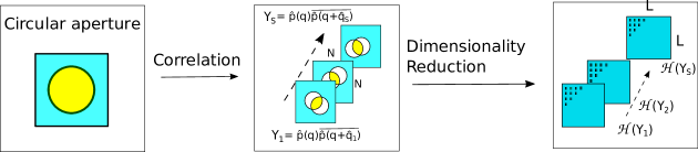
Figure 7: Schematic diagram for pre-computed Wiener filter.

Algorithm 1 Pre-computed Wiener filter for Live WDD

1:Initialization:

1. Initial probe on the Fourier space $\left(p_{ij}\right)=\hat{p}\left(\mathbf{q}\right)$, for $i,j\in[N]$ i.e., circular apperture, generated from the radius of diffraction patterns.

2. Choose a small number to avoid zero division $\epsilon$

2:for each pre-defined index on the spatial frequency coordinate in the set $v\in\{1,2,\dots,S\}$ do

3:      Apply transformation to get physical coordinates of spatial frequency from acquisition setting $\{\hat{\mathbf{q}}_{1},\hat{\mathbf{q}}_{2},\dots,\hat{\mathbf{q}}_{S}\}$

4:      Construct autocorrelation matrix $\mathbf{Y}_{v}\in\mathbb{C}^{N\times N}$ for $v\in[S]$. The element of the matrix is $\left(y_{ij}\right)_{v}=\hat{p}\left(\mathbf{q}\right)\overline{\hat{p}\left(\mathbf{q}+\hat{\mathbf{q}}_{v}\right)}\quad\text{for}\quad i,j\in[N].$

5:      Calculate dimensionality reduction to the initial probe’s autocorrelation $\mathcal{H}\left(\mathbf{Y}_{v}\right)$ for $v\in[S].$

6:      Calculate the Wiener filter $\mathbf{K}_{v}=\frac{\overline{\mathcal{H}\left(\mathbf{Y}_{v}\right)}}{\left|\mathcal{H}\left(\mathbf{Y}_{v}\right)\right|^{2}+\epsilon}\in\mathbb{C}^{L\times L}$ for $v\in[S].$

7:end for

In typical cases for electron microscopy where the illumination is a focused convergent beam with an angular range limited by a circular aperture, we calculate the autocorrelation between shifted circular apertures. At some spatial frequencies $\hat{\mathbf{q}}_{v}$ we may not have an intersection at all. These frequencies do not contribute to the reconstruction and can be omitted from the calculation. An illustration is given in Figure 8.

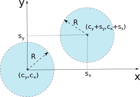
Figure 8: Geometry of the autocorrelation of the probe in reciprocal space.

The shift depends on the microscope and acquisition parameters, such as electron wavelength $\lambda$, semiconvergence angle $\theta$, the radius of the circle in pixel $R$, and the scanning shift on the real space coordinates for both axes $\Delta_{y},\Delta_{x}$. First of all, let us write the condition when the intersection occurs

$$s_{y}^{2}+s_{x}^{2}\leq 4R^{2}$$ (15)

It should be noted that for spatial frequency indexes $v_{y},v_{x}$
$\in[S]$, we can write the transformation to physical coordinate given by

$$s_{y}=v_{y}\frac{\lambda R}{\Delta_{y}S\sin\theta}\quad\text{and}\quad s_{x}=v_{x}\frac{\lambda R}{\Delta_{x}S\sin\theta}$$

If we have the same scanning shift $\Delta_{y}=\Delta_{x}=\Delta$, we can have the condition

$$\left(v_{y}^{2}+v_{x}^{2}\right)\frac{\lambda^{2}}{\Delta^{2}S^{2}\sin^{2}\theta}\leq 4$$ (16)

For all combinations of $v_{y},v_{x}\in[S]$, we can find an upper bound $v_{y}^{2}+v_{x}^{2}\leq 2v^{2}$, where $v=\text{max}\left(v_{y},v_{x}\right)\in[S]$. Hence, we have

$$v\leq\widehat{S}=\frac{\sqrt{2}\Delta\sin\theta}{\lambda}S$$ (17)

For specific setting in the acquisition process, we can have $\frac{\sqrt{2}\Delta\sin\theta}{\lambda}<1$, thereby, only required smaller intersection. To have a concrete number suppose we have a specific value of measurement settings, i.e., $\theta=32$ mrad, $\Delta=0.026$ nm, $\lambda=2.508$ pm, we have scaling factor $\hat{S}=0.47S$, which is smaller than the total spatial frequency index $S$ and can be used to improve the computation time of live processing WDD.

Algorithm 2 Modified WDD

1:Initialization:

1. Pre-compute Wiener filter $\mathbf{K}_{v}$ for $v\in[S]$ given in Algorithm 1 with the number of intersection index $\widehat{S}\leq S$ with applied dimensionality reduction.

2. Initialize source for sequence of diffraction patterns $\mathbf{I}_{s}\in\mathbb{R}^{N\times N}$ for each scanning point $s\in[S]$.

3. Pre-compute DFT matrices $\mathbf{F_{y}}\in\mathbb{C}^{S_{y}\times S_{y}}$ and $\mathbf{F_{x}}\in\mathbb{C}^{S_{x}\times S_{x}}$ for efficient on-the-fly computation of subsets of $\mathbf{F}_{2D}$.

4. Allocate and initialize buffer for object function $\mathbf{O}\in\mathbb{C}^{S_{y}\times S_{x}}$ with zero.

2:for each given real space scanning point index $s$ in the set $\{1,2,\dots,S\}$ do

3:      Apply dimensionality reduction $\mathcal{H}\left(\mathbf{I}_{s}\right)\in\mathbb{R}^{L\times L}$ and vectorization to have $\mathbf{i}_{s}=\text{vec}\left(\mathcal{H}\left(\mathbf{I}_{s}\right)\right)\in\mathbb{R}^{L^{2}}$.

4:      Calculate subset of the Fourier matrix $\mathbf{F}_{2D}$ for $s$ from the two pre-computed DFT matrices.

5:      Calculate outer product between all column element in the subset of the Fourier matrix $\mathbf{F}_{2D}$ and vectorized intensity $\mathbf{i}_{s}$ as in (14), $\mathbf{T}=\mathbf{f}_{s}\mathbf{i}_{s}^{T}\\ \in\mathbb{C}^{S\times L^{2}}$, where we have $\mathbf{t}_{v}\in\mathbb{C}^{L^{2}}$ for $v\in[S]$ for each row of matrix $\mathbf{T}$.

6:     for each given spatial frequency index with non-   zero intersection $v$ in the set $\{1,2,\dots,\widehat{S}\}$ do

7:          Reshape the result for each row, i.e., $\text{mat}\left(\mathbf{t}_{v}\right)\in\mathbb{C}^{L\times L}$.

8:          Deconvolution process on compressed space $\mathbf{D}_{v}=\text{mat}\left(\mathbf{t}_{v}\right)\circ\mathbf{K}_{v}\in\mathbb{C}^{L\times L}$ for $v\in[\widehat{S}]$.

9:          Calculate zero frequency by summing all elements of matrix $\mathbf{D}_{v}=\left(d_{lk}\right)_{v}$ for $l,k\in[L]$. Here we have scalar for each spatial frequency $o_{v}={\sum_{l=1}^{L}\sum_{k=1}^{L}\left(d_{lk}\right)_{v}}$

10:          Replace the element of the non-zero index in spatial frequency with $o_{v}$

11:     end for

12:      We have an update vector $\mathbf{o}=\left(o_{1},o_{2},\dots,o_{S}\right)\in\mathbb{C}^{S}$. This is added to the buffer allocation matrix for each given scanning point $\mathbf{O}:=\mathbf{O}+\text{mat}\left(\mathbf{o}\right)\in\mathbb{C}^{S_{y}\times S_{x}}$

13:end for

14: Applying inverse Fourier transform and complex conjugate on set of spatial frequencies to get real space coordinate of the specimen transfer function $\overline{\mathcal{F}^{-1}\left(\mathbf{O}\right)}$

6.3 Modified WDD

Combining dimensionality reduction, gradual processing, as well as the pre-computed Wiener filter, we present the modified WDD for live reconstruction in Algorithm 2. Since we compress and process the diffraction patterns per scanning point in Algorithm 2, the total reconstruction of the specimen transfer function is updated gradually, starting from a zero-initialized matrix. Furthermore, the updates from subsets of the input data can be computed independently, which allows trivial parallelization. This algorithm for Live WDD is implemented as a User Defined Function (UDF) for LiberTEM-live (Clausen et al., 2020). The complete schematic diagram for an implementation of WDD as a LiberTEM UDF is presented in Figure 9. It is available as Open Source at https://github.com/Ptychography-4-0/LiveWDD.

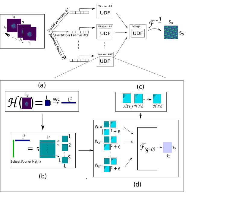
Figure 9: The schematic diagram for running the Live WDD as a UDF in LiberTEM-live. The data stream from the detector is split into partitions, which are streamed to worker processes via queues. Each diffraction pattern is processed in the UDF as follows: (a) Applying dimensionality reduction and vectorization, (b) Processing the compressed frame with a subset of the Fourier matrix, (c) Accessing the pre-computed Wiener filter to perform a single reconstruction as presented in (d). The merge function sums up the contributions from each partition, and the final reconstruction in real space is determined by the two-dimensional inverse Fourier transform.

7 Time and Space Complexity

Here we discuss the analysis of the Live WDD algorithm and compare it with conventional WDD. For both approaches, we derive the time and space complexity required to perform the steps specified by the algorithm. In this section, we denote the total scanning points as $S$ for raster position on both $x,y$ axis, i.e., $S=S_{x}\times S_{y}$. In addition, the dimension of the detector is denoted as $N\times N$. In Table 1 we provide a summary for the time and space complexity analysis for both algorithms.

Table 1: Computational complexity of conventional WDD and Live WDD

Complexity	Conventional WDD	Live WDD
Time	$\mathcal{O}\left(SN^{2}\log SN^{2}\right)$	$\text{max}\left(\mathcal{O}(SN^{2}L),\mathcal{O}(S^{2}L^{2})\right)$
Space	$\mathcal{O}\left(SN^{2}\right)$	$\mathcal{O}({S}L^{2})$

For space complexity it appears that the Live WDD scales better compared to conventional WDD since $L\ll N$. However, for time complexity it highly depends on the total scanning points $S$ and the logarithmic factor $\log(SN^{2})$ compared to the low dimension $L$, here we use $L=16$. The derivation of complexity analysis is provided in Section 7.1 and Section 7.2, respectively.

7.1 Conventional WDD

First of all, conventional WDD performs a Fourier transform along the scanning position in real space to obtain the spatial frequencies. The computational complexity of a fast Fourier transform for all scanning points is $\mathcal{O}(SN^{2}\\ \log S)$. For each spatial frequency, we calculate the autocorrelation of the probe, which gives us computation time $\mathcal{O}\left(N^{2}\right)$. Afterward, we calculate the Wigner distribution function by applying inverse Fourier transform on the autocorrelation as well as the intensity of diffraction patterns, for each taking $\mathcal{O}\left(N^{2}\log N^{2}\right)$. The process is followed by applying Wiener filtering or deconvolution that requires $\mathcal{O}\left(N^{2}\right)$. Since we have to calculate all spatial frequencies, the computation is therefore $S\left(\mathcal{O}(N^{2}\right)+\mathcal{O}(N^{2}\log N^{2}))$, which gives total for processing all spatial frequencies $\mathcal{O}\left(SN^{2}\log N^{2}\right)$. The next step is to calculate the Fourier transform of all deconvolution data before taking only zero reciprocal space, i.e., $\mathbf{q}=0$, hence we perform operation $\mathcal{O}\left(SN^{2}\log N^{2}\right)$. In the last step, we apply an inverse Fourier transform for estimated object which requires $\mathcal{O}\left(S\log S\right)$. The total time computation for conventional WDD then $\mathcal{O}\left(SN^{2}\log(S)\right)+\mathcal{O}\left(SN^{2}\log N^{2}\right)+\mathcal{O}\left(S\log S\right)$. Simplification gives us time complexity of conventional WDD as $\mathcal{O}\left(SN^{2}\log SN^{2}\right)$.

For space complexity, we start with total memory allocation to store all four-dimensional datasets to perform a Fourier transform on scanning points on the real space, i.e., to obtain the spatial frequencies, which requires
$\mathcal{O}\left(SN^{2}\right)$. For each spatial frequency, we have to process the data with dimension $\mathcal{O}\left(N^{2}\right)$. In the last process to calculate the estimated object we have space complexity $\mathcal{O}\left(S\right)$. Thereby, total space complexity of conventional WDD is $\mathcal{O}\left(SN^{2}\right)+\mathcal{O}\left(N^{2}\right)+\mathcal{O}\left(S\right)$, which then we have scaling for space complexity $\mathcal{O}\left(SN^{2}\right)$.

7.2 Live WDD

The Live WDD presented here includes a compression step where the dimension of the compressed data is $L\times L$, much smaller than detector size ($L\ll N$). For the time complexity of Live WDD, we separate the processing into the computation of the Wiener filter in Algorithm 1 and the actual data processing. The Wiener filter requires $\mathcal{O}(N^{2})$ for computing the autocorrelation function. Since we apply a dimensionality reduction, which is performed with three matrix multiplications, we have $\mathcal{O}(LN^{2}+L^{2}N)$. At the end of the process, we compute the element-wise division for the Wiener filter with complexity $\mathcal{O}(L^{2})$ and incorporate the process for all spatial frequencies $S$. Therefore, we have time complexity for the pre-computed Wiener filter as $\mathcal{O}({S}N^{2}L)$. For processing each scanning point, we calculate the dimensionality reduction for each diffraction pattern with complexity $\mathcal{O}(L^{2}N+N^{2}L)$. Afterward, the computation of the outer product between each column of Fourier matrix with a compressed diffraction pattern requires $\mathcal{O}\left(SL^{2}\right)$. The next process is the deconvolution with the pre-computed Wiener filter for all spatial frequencies which takes $\mathcal{O}\left(SL^{2}\right)$. Getting zero frequencies and the update data have complexity $\mathcal{O}\left(SL^{2}\right)$ and $\mathcal{O}\left(S\right)$, respectively. Thereby, processing with all real space scanning points is given by $\mathcal{O}(SL^{2}N+SN^{2}L)+\mathcal{O}(S^{2}L^{2})+\mathcal{O}(S^{2})$. In the last step, to get the estimated object on the real space with dimension $S$, we apply an inverse Fourier transform that requires $\mathcal{O}\left(S\log S\right)$.

In the end, for Live WDD we have total time complexity $\mathcal{O}\left(SL^{2}N+SN^{2}L\right)+\mathcal{O}(S^{2}L^{2})+\mathcal{O}(S^{2})+\mathcal{O}\left(S\log S\right)$, which then gives us $\text{max}\left(\mathcal{O}(SN^{2}L),\mathcal{O}(S^{2}L^{2})\right)$. The result highly depends on the dimension of $N$ and ${S}$, where for a larger detector dimension than total spatial frequency, we have time complexity $\mathcal{O}\left(SN^{2}L\right)$. On the contrary, if we have a large field of view, there is a possibility then we have time complexity $\mathcal{O}\left(S^{2}L^{2}\right)$.

Regarding the space complexity, in Live WDD we can process the data per frame, i.e. per diffraction pattern, the size of which corresponds to the detector’s dimension. In comparison, conventional WDD stores the complete four-dimensional dataset to compute the spatial frequencies. In addition, we apply a dimensional reduction technique that only requires $\mathcal{O}\left(L^{2}\right)$. For each scanning point on the real space as well as the non-zero intersection on the spatial frequency, the algorithm only requires $\mathcal{O}(L^{2})$ except for computing the estimated object that has dimension $\mathcal{O}(S)$. For the pre-computed Wiener filter, we have to store $\widehat{S}\leq S$ non-zero intersection spatial frequencies for the autocorrelation process with compressed dimension $L\times L$. Hence we have $\mathcal{O}({S}L^{2})$ space complexity of the pre-computed Wiener filter. In total we have $\mathcal{O}({S}L^{2})+\mathcal{O}(S)+\mathcal{O}(L^{2})$ and give us complexity $\mathcal{O}({S}L^{2})$, which still better than conventional WDD.

In Section 9, we compare real-world time and space use of the proposed Live WDD and conventional WDD on various datasets.

8 Simulation and Experimental Datasets

The information of datasets and parameter settings to evaluate Live WDD are given in (Pennycook, 2021) for simulated graphene. The specimen has a hexagonal lattice structure, shown in Figure 10. The four-dimensional STEM data are generated by parameter settings presented in Table 2.

Table 2: Parameters for simulated graphene (Pennycook, 2021)

Parameters	Graphene
Rotation (deg)	$0.0$
Semiconv. angle (mrad)	$30$
Accel. voltage (keV)	$60$
Scanning step size (nm)	$0.02$
Scanning points (Sy, Sx)	$\left(64,65\right)$
Detector size (pixel)	$\left(256,256\right)$

We can also add the effect of Poissonian noise to the simulated diffraction patterns data. Suppose we have dose level per pixel represented by variable $\nu$ that has a unit $\,e^{-}/$Ų . The model used to generate a noisy dataset for each intensity of diffraction patterns $\mathbf{I}_{s}\in\mathbb{R}^{N\times N}$ for $s\in[S]$ is given as follows

$$\texttt{Poisson}\left(\nu\mathbf{\widetilde{I}}_{s}\right)\in\mathbb{R}^{N\times N},$$

where the $\mathbf{\widetilde{I}}_{s}$ is normalisation of the diffraction pattern for each scanning point and Poisson is a function to generate Poisson distribution applied to our dataset. It should be noted that this function preserves the dimension of the data.

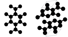
Figure 10: Structure of graphene. The structure is downloaded from materialsproject.org(Jain et al., 2013)

Additionally, we also used an experimental datasets of SrTiO₃ specimen acquired using Medipix Merlin EM detector (Strauch et al., 2021a), where the structure is presented in Figure 11. The parameters setting of this dataset is presented in Table 3. Complete information about this dataset can be directly seen (Strauch et al., 2021a).

Figure 11: Structure of SrTiO₃ where Strontium, Titanium, and Oxygen are visualized as white, purple, and red colors. The structure is downloaded from materialsproject.org(Jain et al., 2013)

Table 3: Parameters for experimental dataset SrTiO₃ (Strauch et al., 2021a)

Parameters	SrTiO3
Rotation (deg)	$88$
Semiconv. angle (mrad)	$22.13$
Accel. voltage (keV)	$300$
Scanning step size (nm)	$0.0127$
Scanning points (Sy, Sx)	$\left(128,128\right)$
Detector size (pixel)	$\left(256,256\right)$

9 Numerical Results

We present numerical evaluations of the Live WDD in terms of reconstruction, computation time, and memory allocation. For Live WDD, we also present how the live reconstruction evolves from partial results. As a comparison to the existing WDD implementation, we refer to the implementation in (Yang et al., 2016) as the reference to check the dynamic range of the phase, where the source code is available in https://gitlab.com/ptychoSTEM/ptychoSTEM and https://gitlab.com/PyPtychoSTEM/PyPtychoSTEM. We use the same reconstruction parameters in WDD as given in the source code, for instance, the small constant $\epsilon$ for the Wiener filter.

The evaluation is performed individually on the same workstation with AMD EPYC 7543P with $32$ CPU with $64$ threads operating at a base frequency of $2.80$  GHz, and $512$  GB DDR4 RAM with an operating frequency of $3.2$  GHz. It should be noted that the simulation for each algorithm is performed without a noise background, i.e., no other processes or algorithms were running during the evaluation.

9.1 Reconstruction

In this section, we performed numerical comparisons of the Live WDD and the conventional WDD given in the PyPtychoSTEM, with a similar setting for both algorithms, e.g., $\epsilon=0.01$. In the first part, we focus on the evaluation of noise-free conditions for graphene datasets. The second part covers the performance of algorithms when applied to data that is degraded by Poissonian noise corresponding to different dose levels. Since the goal is to show the specimen transfer functions, we present the final phase reconstruction from the Live WDD.

Figure 12: Phase reconstruction of simulated graphene with (a). PyPtychoSTEM and (b). Live Processing WDD

Figure 12 shows the reconstruction of the graphene dataset for both the PyPtychoSTEM implementation of WDD and the Live WDD for noise-free conditions. It can be seen that the Live WDD can reconstruct the specimen transfer function with the correct orientation of the atom represented by the phase and similar dynamic range. In the next evaluation, we conduct numerical evaluation for different dose levels, namely for $\nu\in\{10^{2},10^{3},10^{4},10^{5}\}$
$\,e^{-}/$Ų. The reconstruction for noisy setting is depicted in Figure 13.

Figure 13: Phase reconstruction of simulated graphene with different dose levels (a) $10^{2}\,e^{-}/$Ų, (b) $10^{3}\,e^{-}/$Ų,(c) $10^{4}\,e^{-}/$Ų, (d) $10^{5}\,e^{-}/$Ų

Compared to the conventional WDD, which performs faithful reconstruction starting from dose $\nu=10^{5}\,e^{-}/$Ų, Live WDD yields a recognizable reconstruction starting from $\nu=10^{4}\,e^{-}/$Ų. Hence, it can be seen that the Live WDD is more robust against Poissonian noise. Besides the property of flexible dimensional reduction, the arbitrary order of the Hermite-Gauss functions can be seen as a low-pass filter, where the width $\sigma$ is optimized so that the any pixel noise is strongly suppressed by the dimensionality reduction, as in Figure 5.

A line scan through the reconstruction at dose level $10^{4}\,e^{-}/$Ų is presented in Figure 14, which shows that the noise affects the phase reconstruction of both algorithms. It can be seen that the Live WDD has better noise suppression than PyPtychoSTEM, where the latter requires more dose to reliably find atom positions in the phase reconstruction. For infinite dose, both algorithms present the same atom positions with a different value range for Live WDD compared to PyPtychoSTEM. A difference is to be expected because Live WDD reduces the dimensionality using Hermite-Gauss functions, while PyPtychoSTEM uses Fourier space without dimensionality reduction. That means the two methods are not numerically equivalent.

Figure 14: Phase reconstruction of simulated graphene with dose level $10^{4}\,e^{-}/$Ų and infinite dose for both algorithms (a). PyPtychoSTEM and (b). Live WDD. The line scan reconstruction is also presented where the scan location on Y-direction: $32$ is shown with a red line.

9.2 Computation time

The numerical computation time for Live WDD compared to the conventional WDD given in (Yang et al., 2016) is discussed. The evaluation is presented in Table 4 and Table 5, where we measure the median, as well as the standar deviation of computation time for live and conventional WDD for different dimension of datasets generated from Graphene in (Pennycook, 2021).

Table 4: Numerical median computation time in seconds for PyPtychoSTEM and Live WDD for fixed dimension scanning points $S_{y}=S_{x}=128$ and increasing detector $N_{y}=N_{x}$.

Dimension	PyPtychoSTEM	Live WDD
$128$	$48.76\pm 0.14$	$1.28\pm 0.07$
$256$	$145.51\pm 2.16$	$2.21\pm 0.069$
$512$	$631.71\pm 9.05$	$12.60\pm 0.65$
$1024$	$-$	$37.42\pm 0.85$

To investigate the effect of both increasing scanning points and detector dimensions on the computation time, we also observe both parameter settings, where we use the convention $S_{y},S_{x}$ as the number of scanning points for both axes in the raster scan. Dimension of detector is given by $N_{y},N_{x}$.

We perform $10$ trials to measure the numerical computation time for both algorithms. From these measurements we show the median computation time. It can be seen that PyPtychoSTEM requires more memory than available to accomplish the reconstruction. As discussed in the Section 7, accommodating an entire dataset requires a large memory allocation for PyPtychoSTEM and impinges on the computation performance in general.

Table 5: Numerical median computation time in seconds for PyPtychoSTEM and Live WDD for fixed dimension detector $N_{y}=N_{x}=128$ and increasing scanning points $S_{y}=S_{x}$.

Dimension	PyPtychoSTEM	Live WDD
$128$	$48.76\pm 0.14$	$1.28\pm 0.07$
$256$	$199.12\pm 0.60$	$14.82\pm 0.05$
$512$	$824.04\pm 7.45$	$228.59\pm 0.18$
$1024$	$-$	$3048.48\pm 5.94$

In all cases, Live WDD performs faster numerical computation than conventional WDD implemented in PyPtychoSTEM. However, when the same dimension for both scanning points and detector size is evaluated, i.e., $(1024,\\ 1024)$, we observe the computation time increases approximately a hundred-fold due to the quadratic scaling in the time complexity, as discussed in Section 7.

9.3 Memory allocation

Apart from the numerical computation time, we are also interested in independently observing the memory allocation for both algorithms during the reconstruction process. For this reason, we record the memory usage every $0.2$ seconds. The evaluation for memory allocation is also performed independently of the investigation of numerical computation time in the previous section and separately for each algorithm. Similar to the numerical computation time, we present the evaluation for both increasing dimensions of scanning points and detector.

Figure 15: Memory allocation for conventional WDD and Live WDD for different detector sizes: (a). (128,128,128,128), (b). (128,128,256,256), (c). (128,128,512,512), (d). (128,128,1024,1024).

Figure 15 shows that for detector dimension $(1024,\\ 1024)$ PyPtychoSTEM requires more memory than available to complete the reconstruction. Live WDD only requires a constant amount of memory around $10^{4}$ MB independent of detector size.

Table 6: Maximum memory allocation in MB for PyPtychoSTEM and Live WDD for fixed scanning points dimension $S_{y}=S_{x}=128$ and increasing detector size $N_{y}=N_{x}$.

Dimension	PyPtychoSTEM	Live WDD
$128$	$14725$	$15343$
$256$	$60505$	$16136$
$512$	$244557$	$17889$
$1024$	$-$	$24887$

The maximum memory allocation to complete each algorithm for increasing detector dimension is presented in Table 6.

Figure 16: Memory allocation for conventional WDD and Live WDD for different scanning point dimensions: (a).(128,128,128,128), (b).(256,256,128,128), (c).(512,512,128,128), (d).(1024,1024,128,128)

In addition, we also investigate the effect of increasing scanning points dimension or the dimension of the field of view, as presented in Figure 16. PyPtychoSTEM requires more memory than available to complete the reconstruction for scanning points $(1024,1024)$. Also in this scenario, Live WDD uses memory more efficiently than PyPtychoSTEM. The maximum memory allocation for increasing scanning points is given in Table 7.

Table 7: Maximum memory allocation in MB for PyPtychoSTEM and Live WDD for fixed dimension detector $N_{y}=N_{x}=128$ and increasing scanning points $S_{y}=S_{x}$.

Dimension	PyPtychoSTEM	Live WDD
$128$	$14725$	$15343$
$256$	$61521$	$19952$
$512$	$244121$	$39577$
$1024$	$-$	$106585$

9.4 Live processing evaluation

In this section, we demonstrate that the performance of Live WDD is sufficient for live acquisition and reconstruction with real-world 4D STEM detectors. In 4D STEM, illustrated in Figure 1, the acquisition time per scanning point is usually limited by the detector frame rate. The specification for different detectors, namely Merlin MedipixEM , Dectris Quadro, and Dectris Arina, are given in Table 8. The maximum frame rate may depend on the chosen bit depth and readout area for a given detector.

Table 8: Specification of different detectors that support experimental acquisition

Detectors	Frame rate (kHz)
MedipixEM	18.8 (1-bit), 3.2 (6-bit), or 1.6 (12-bit)
Dectris Quadro	2.25 (16-bit), 4.5 (8-bit), ROI 9 (16-bit),
	ROI 18 (8-bit)
Dectris Arina	120

To accomplish a continuous reconstruction, data processing time per detector frame needs to be faster than the STEM dwell time. Following the considerations on computational complexity, this highly depends on the number of scanning points, the detector size, and the number of non-zero entries in the Wiener filter. Since the processing is parallelized using a UDF and LiberTEM-live, the number and speed of CPU cores is a major factor as well.

To illustrate the scalability of Live WDD, we show the scaling behavior of the computation time as a function of number of CPU cores for dimension $\left(128,128,128,128\right)$, as presented in Figure 17. The scaling is nearly linear for up to eight cores and tapers off after that.

Table 9: Processing speed in frames per second for Live WDD for fixed dimension detector $N_{y}=N_{x}=128$ and increasing scanning points $S_{y}=S_{x}$.

Dimension	Average (sec)	Frame/sec
$128$	$1.32$	$12412$
$256$	$14.82$	$4422$
$512$	$228.65$	$1146$
$1024$	$3048.66$	$343$

Figure 17: Computation time depending on the number of cores for a dataset dimension $(128,128,128,128)$. Despite using the CPU bandwidth as a shared resource the algorithm exhibits a $15\times$ speedup on 32 cores.

Based on the performance data from our $32$ core CPU in Tables 4 and 5, we can therefore support live reconstruction up to the frames per second (fps) as presented in Table 9. Therefore, a reconstruction using Live WDD can keep up with Merlin Medipix and Dectris Quadro without ROI up to a dimension of $\left(256,256,128,128\right)$ when used with the given setup and settings.

Figure 18 shows simulated live reconstruction for different stages of scanning progress for Live WDD and Live SSB from (Strauch et al., 2021b), where the update is added gradually until completing all scanning points. Here the dimension of the four-dimensional STEM data is
$\left(128,128,256,256\right)$, as described in Table 3.

Figure 18: Snapshots of simulated live ptychography (phase) using Live WDD (Top) and Live SSB (Bottom) method at different stages of the scan for SrTiO₃ datasets for different buffer processes: (a) 10, (b) 26, (c) 41, (d) 57, (e) 72. Note how the results don’t have to be merged in any particular order.

10 Discussion

Since we only perform the object reconstruction using a synthetic probe initialization, a potential next step for Live WDD could be to factor in the microscope alignment and update the probe. After estimating the object, we can swap the deconvolution process to reconstruct the probe. This process is straightforward, but the additional computation and update for the Wiener filter would affect the performance. Therefore, an efficient and on-fly computation should be implemented to overcome this issue.

The time complexity of Live WDD for a large field of view is scaled quadratically with total scanning points and reduced dimension, respectively. Although the Live WDD implementation can complete the reconstruction, our numerical observation shows that it takes approximately one hour with dimension $(1024,1024,128,128)$, which is inefficient. This could be overcome by subdividing the field of view into smaller patches that are reconstructed independently and subsequently merged. In this case, the time complexity can be reduced to a linear scale of the number of subsets.

Another strategy to optimize the performance of Live WDD could be to choose an optimal scan step based on the intersection of the probe’s auto correlation in reciprocal space, as presented in (17). Making sure that the scan grid is not unnecessarily fine can reducing the number of scanning points to process.

It is also thinkable to adapt WDD and Live WDD for scan patterns that are not on an equispaced grid. In that case a matrix for a non-uniform discrete Fourier transform should be used to match the scanning points. We will defer such possible improvements to future works.

11 Summary

As an evolution of the classical WDD algorithm, we demonstrated Live WDD that can reconstruct in a streaming fashion while acquiring diffraction patterns to support real-time reconstruction. Our investigation shows that Live WDD produces object reconstructions that approximate the conventional result. The algorithm uses less memory and runs faster than the classical WDD for typical parameters. As a side effect of dimensionality reduction, we also observe that it acts as a filter for Poissonian noise to attain a more robust reconstruction from low-dose diffraction patterns. We compare the numerical computation time of the proposed algorithm with the dwell time of Merlin Medipix and Dectris Quadro detectors, where we can perform live continuous reconstruction with a field of view up to $(256,256)$ on a system with 32 CPU cores.

References

- Bostan et al. (2018) Bostan, E., Soltanolkotabi, M., Ren, D. & Waller, L. (2018). Accelerated wirtinger flow for multiplexed fourier ptychographic microscopy, 2018 25th IEEE International Conference on Image Processing (ICIP), 3823–3827, IEEE.
- Clausen et al. (2020) Clausen, A., Weber, D., Ruzaeva, K., Migunov, V., Baburajan, A., Bahuleyan, A., Caron, J., Chandra, R., Halder, S., Nord, M. et al. (2020). LiberTEM: Software platform for scalable multidimensional data processing in transmission electron microscopy, Journal of Open Source Software 5, 2006.
- Glaeske (1983) Glaeske, H. (1983). On a convolution structure of a generalized Hermite transformation, Serdica Bulgaricae Math Publ 9, 223–229.
- Golub & Van Loan (2013) Golub, G.H. & Van Loan, C.F. (2013). Matrix computations, JHU press.
- Hoppe (1969a) Hoppe, W. (1969a). Beugung im inhomogenen Primärstrahlwellenfeld. I. Prinzip einer Phasenmessung von Elektronenbeungungsinterferenzen, Acta Crystallographica Section A 25, 495–501, URL https://doi.org/10.1107/S0567739469001045.
- Hoppe (1969b) Hoppe, W. (1969b). Beugung im inhomogenen Primärstrahlwellenfeld. III. Amplituden- und Phasenbestimmung bei unperiodischen Objekten, Acta Crystallographica Section A 25, 508–514, URL https://doi.org/10.1107/S0567739469001069.
- Hoppe & Strube (1969) Hoppe, W. & Strube, G. (1969). Beugung in inhomogenen Primärstrahlenwellenfeld. II. Lichtoptische Analogieversuche zur Phasenmessung von Gitterinterferenzen, Acta Crystallographica Section A 25, 502–507, URL https://doi.org/10.1107/S0567739469001057.
- Jain et al. (2013) Jain, A., Ong, S.P., Hautier, G., Chen, W., Richards, W.D., Dacek, S., Cholia, S., Gunter, D., Skinner, D., Ceder, G. et al. (2013). Commentary: The materials project: A materials genome approach to accelerating materials innovation, APL materials 1, 011002.
- Jain (1989) Jain, A.K. (1989). Fundamentals of digital image processing, Prentice-Hall, Inc.
- Li et al. (2014) Li, P., Edo, T.B. & Rodenburg, J.M. (2014). Ptychographic inversion via Wigner distribution deconvolution: Noise suppression and probe design, Ultramicroscopy 147, 106–113.
- Maiden & Rodenburg (2009) Maiden, A.M. & Rodenburg, J.M. (2009). An improved ptychographical phase retrieval algorithm for diffractive imaging, Ultramicroscopy 109, 1256–1262.
- Nord et al. (2020) Nord, M., Webster, R.W., Paton, K.A., McVitie, S., McGrouther, D., MacLaren, I. & Paterson, G.W. (2020). Fast pixelated detectors in scanning transmission electron microscopy. part i: data acquisition, live processing, and storage, Microscopy and Microanalysis 26, 653–666.
- Ophus (2019) Ophus, C. (2019). Four-Dimensional Scanning Transmission Electron Microscopy (4D-STEM): From Scanning Nanodiffraction to Ptychography and Beyond, Microscopy and Microanalysis 25, 563–582.
- Pelz et al. (2021) Pelz, P.M., Johnson, I., Ophus, C., Ercius, P. & Scott, M.C. (2021). Real-time interactive 4D-STEM phase-contrast imaging from electron event representation data: Less computation with the right representation, IEEE Signal Processing Magazine 39, 25–31.
- Pennycook (2021) Pennycook, T. (2021). Graphene simulated dataset, Zenodo URL https://doi.org/10.5281/zenodo.4476506.
- Pennycook & Hofer (2021) Pennycook, T. & Hofer, C. (2021). PyPtychoSTEM, Online, URL https://gitlab.com/pyptychostem/pyptychostem/.
- Pennycook et al. (2015) Pennycook, T.J., Lupini, A.R., Yang, H., Murfitt, M.F., Jones, L. & Nellist, P.D. (2015). Efficient phase contrast imaging in STEM using a pixelated detector. part 1: Experimental demonstration at atomic resolution, Ultramicroscopy 151, 160–167.
- Rodenburg & Bates (1992) Rodenburg, J. & Bates, R. (1992). The theory of super-resolution electron microscopy via Wigner-distribution deconvolution, Philosophical Transactions of the Royal Society of London Series A: Physical and Engineering Sciences 339, 521–553.
- Rodenburg et al. (1993) Rodenburg, J., McCallum, B. & Nellist, P. (1993). Experimental tests on double-resolution coherent imaging via STEM, Ultramicroscopy 48, 304–314, URL https://www.sciencedirect.com/science/article/pii/0304399193901057.
- Rodenburg & Faulkner (2004) Rodenburg, J.M. & Faulkner, H.M. (2004). A phase retrieval algorithm for shifting illumination, Applied physics letters 85, 4795–4797.
- Sakurai (1994) Sakurai, J.J. (1994). Modern quantum mechanics; rev. ed., Reading, MA: Addison-Wesley.
- Spurgeon et al. (2021) Spurgeon, S.R., Ophus, C., Jones, L., Petford-Long, A., Kalinin, S.V., Olszta, M.J., Dunin-Borkowski, R.E., Salmon, N., Hattar, K., Yang, W.C.D. et al. (2021). Towards data-driven next-generation transmission electron microscopy, Nature materials 20, 274–279.
- Strauch et al. (2021a) Strauch, A., Clausen, A., Müller-Caspary, K. & Weber, D. (2021a). High-resolution 4D STEM dataset of SrTiO3 along the [1 0 0] axis at high magnification, Tech. rep., Physik Nanoskaliger Systeme.
- Strauch et al. (2021b) Strauch, A., Weber, D., Clausen, A., Lesnichaia, A., Bangun, A., März, B., Lyu, F.J., Chen, Q., Rosenauer, A., Dunin-Borkowski, R. & et al. (2021b). Live processing of momentum-resolved STEM data for first moment imaging and ptychography, Microscopy and Microanalysis 1–15.
- Wen et al. (2012) Wen, Z., Yang, C., Liu, X. & Marchesini, S. (2012). Alternating direction methods for classical and ptychographic phase retrieval, Inverse Problems 28, 115010.
- Yang et al. (2017) Yang, H., MacLaren, I., Jones, L., Martinez, G.T., Simson, M., Huth, M., Ryll, H., Soltau, H., Sagawa, R., Kondo, Y. et al. (2017). Electron ptychographic phase imaging of light elements in crystalline materials using Wigner distribution deconvolution, Ultramicroscopy 180, 173–179.
- Yang et al. (2015) Yang, H., Pennycook, T.J. & Nellist, P.D. (2015). Efficient phase contrast imaging in STEM using a pixelated detector. part ii: Optimisation of imaging conditions, Ultramicroscopy 151, 232–239.
- Yang et al. (2016) Yang, H., Rutte, R., Jones, L., Simson, M., Sagawa, R., Ryll, H., Huth, M., Pennycook, T., Green, M., Soltau, H. et al. (2016). Simultaneous atomic-resolution electron ptychography and z-contrast imaging of light and heavy elements in complex nanostructures, Nature Communications 7, 1–8.
- Yu et al. (2021) Yu, C.P., Friedrich, T., Jannis, D., Van Aert, S. & Verbeeck, J. (2021). Real-time integration center of mass (ricom) reconstruction for 4d stem, Microscopy and Microanalysis 1–12.