ViTAL: Vision-Based Terrain-Aware Locomotion
for Legged Robots

Abstract

This work is on vision-based planning strategies for legged robots that separate locomotion planning into foothold selection and pose adaptation. Current pose adaptation strategies optimize the robot’s body pose relative to given footholds. If these footholds are not reached, the robot may end up in a state with no reachable safe footholds. Therefore, we present a Vision-Based Terrain-Aware Locomotion (ViTAL) strategy that consists of novel pose adaptation and foothold selection algorithms. ViTAL introduces a different paradigm in pose adaptation that does not optimize the body pose relative to given footholds, but the body pose that maximizes the chances of the legs in reaching safe footholds. ViTAL plans footholds and poses based on skills that characterize the robot’s capabilities and its terrain-awareness. We use the 90 kg HyQ and 140 kg HyQReal quadruped robots to validate ViTAL, and show that they are able to climb various obstacles including stairs, gaps, and rough terrains at different speeds and gaits. We compare ViTAL with a baseline strategy that selects the robot pose based on given selected footholds, and show that ViTAL outperforms the baseline.

I Introduction

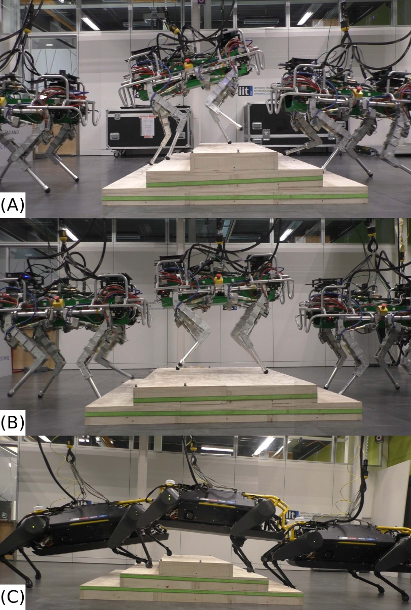
Legged robots have shown remarkable agile capabilities in academia [1, 2, 3, 4, 5, 6] and industry [7, 8, 9]. Yet, to accomplish breakthroughs in dynamic whole-body locomotion, and to robustly traverse unexplored environments, legged robots have to be terrain aware. Terrain-Aware Locomotion (TAL) implies that the robot is capable of taking decisions based on the terrain [10]. The decisions can be in planning, control, or in state estimation, and the terrain may vary in its geometry and physical properties [11, 12, 13, 14, 15, 16, 17, 18, 19]. TAL allows the robot to use its on-board sensors to perceive its surroundings and act accordingly. This work is on vision-based TAL planning strategies that plan the robot’s motion (body and feet) based on the terrain information that is acquired using vision (see Fig. 1).

Figure 1: The HyQ and HyQReal quadruped robots climbing stairs using ViTAL.

I-A Related Work - Vision-Based Locomotion Planning

Vision-based locomotion planning can either be coupled or decoupled. The coupled approach jointly plans the body pose and footholds in a single algorithm. The decoupled approach independently plans the body pose and footholds in separate algorithms. The challenge in the coupled approach is that it is computationally expensive to solve in real-time. Because of this, the decoupled approach tends to be more practical since the high-dimensional planning problem is split into multiple low-dimensional problems. This also makes the locomotion planning problem more tractable. However, this raises an issue with the decoupled approach because the plans may conflict with each other since they are planned separately. Note that both approaches could be solved using optimization, learning, or heuristic methods.

Trajectory Optimization (TO) is one way to deal with coupled vision-based locomotion planning. By casting locomotion planning as an optimal control problem, TO methods can optimize the robot’s motion while taking into account the terrain information [20, 21, 22, 23, 24]. The locomotion planner can generate trajectories that prevent the robot from slipping or colliding with the terrain by encoding the terrain’s shape and friction properties in the optimization problem [24]. TO methods can also include a model of the terrain as a cost map in the optimization problem, and generate the robot’s trajectories based on that [25]. TO methods provide guarantees on the optimality and feasibility of the devised motions, albeit being computationally expensive; performing these optimizations in real-time is still a challenge. To overcome this issue, TO approaches often implement hierarchical (decoupled) approaches. Instead of decoupling the plan into body pose and footholds, the hierarchical approaches decouple the plan into short and long-horizon plans [26, 27]. Additionally, other work relies on varying the model complexity to overcome the computational issue with TO [28].

Reinforcement Learning (RL) methods mitigate the computational burden of TO methods by training function approximators that learn the locomotion plan [29, 30, 31, 32, 33, 34, 35]. Once trained, an RL policy can generate body pose and foothold sequences based on proprioceptive and/or visual information. Yet, RL methods may require tedious learning (large amounts of data and training time) given its high-dimensional state representations.

As explained earlier, decoupled locomotion planning can mitigate the problems of TO and RL by separating the locomotion plan into feet planning and body planning [36, 37, 38, 39, 40, 41]. Thus, one can develop a more refined and tractable algorithm for every module separately. In this work, planning the feet motion (foothold locations) is called foothold selection, and planning the body motion is called pose adaptation.

I-B Related Work - Foothold Selection and Pose Adaptation

Foothold selection strategies choose the best footholds based on the terrain information and the robot’s capabilities. Early work on foothold selection was presented by Kolter et al. [42] and Kalakrishnan et al. [43] where both approaches relied on motion capture systems and an expert user to select (label) the footholds. These works were then extended in [44] using unsupervised learning, on-board sensors, and considered the terrain information such as the terrain roughness (to avoid edges and corners) and friction (to avoid slippage). Then, Barasuol et al. [45] extended the aforementioned work by selecting footholds that not only considers the terrain morphology, but also considering leg collisions with the terrain. Further improvements in foothold selection strategies added other evaluation criteria such as the robot’s kinematic limits. These strategies use optimization [37, 46, 47], supervised learning [38, 48, 49], RL [1, 17], or heuristic [50] methods.

Similar to foothold selection, pose adaptation strategies optimize the robot’s body pose based on the terrain information and the robot’s capabilities. An early work on vision-based pose adaptation was presented in [36]. The goal was to find the optimal pose that maximizes the reachability of given selected footholds, avoid collisions with the terrain, and maintain static stability. The given footholds are based on a foothold selection algorithm that considers the terrain geometry. Another approach was presented in [51] that finds the optimal body elevation and inclination given the selected footholds, and the robot location in the map. The pose optimizer maximizes different margins that increase the kinematic reachability of the legs and static stability, and avoids terrain collisions. This approach was then extended in [52] with an improved version of the kinematic margins. A similar approach was presented in [37] where the goal was to find an optimal pose that can maximize the reachability of given selected footholds. The reachability term is accounted for in the cost function of the optimizer by penalizing the difference between the default foothold position and the selected one. The work in [39] builds on top of the pose optimizer of [37] to adapt the pose of the robot in confined spaces using 3D terrain maps. This is done using a hierarchical approach that first samples body poses that allows the robot to navigate through confined spaces, then smooths these poses using a gradient descent method that is then augmented with the pose optimizer of [37]. The work presented in [53] generates vision-based pose references that also rely on given selected footholds to estimate the orientation of the terrain and send it as a pose reference. Alongside the orientation reference, the body height reference is set at a constant vertical distance (parallel to gravity) from the center of the approximated plane that fits through the selected footholds.

The aforementioned pose adaptation strategies focus on finding one optimal solution based on given footholds; footholds have to be first selected and given to the optimizer. Despite selecting footholds that are safe, there are no guarantees on what would happen during execution if the footholds are not reached or if the robot deviates from its planned motion. If any of these cases happen, the robot might end up in a pose where no safe footholds can be reached. This would in turn compromise the safety and performance of the robot. Even if the strategy can re-plan, reaching a safe pose might not be possible if the robot is already in an unsafe state.

I-C Proposed Approach

We propose Vision-Based Terrain-Aware Locomotion (ViTAL), an online whole-body locomotion planning strategy that consists of a foothold selection and a pose adaptation algorithm. The foothold selection algorithm used in this work is an extension of the Vision-Based Foothold Adaptation (VFA) algorithm of the previous work done by Villarreal et al. [38] and Esteban et al. [49]. Most importantly, we propose a novel Vision-Based Pose Adaptation (VPA) algorithm that introduces a different paradigm to overcome the drawbacks of the state-of-the-art pose adaptation methods. Instead of finding body poses that are optimal for given footholds, we propose finding body poses that maximize the chances of reaching safe footholds in the first place. Hence, we are interested in putting the robot in a state in which if it deviates from its planned motion, the robot remains around a set of footholds that are still reachable and safe. The notion of safety emerges from skills that characterize the robot’s capabilities.

ViTAL plans footholds and body poses by sharing the same robot skills (both for the VPA and the VFA). These skills characterize what the robot is capable of doing. The skills include, but are not limited to: the robot’s ability to avoid edges, corners, or gaps (terrain roughness), the robot’s ability to remain within the workspace of the legs during the swing and stance phases (kinematic limits), and the robot’s ability to avoid colliding with the terrain (leg collision). These skills are denoted by Foothold Evaluation Criteria (FEC). Evaluating the FEC is usually computationally expensive. Thus, to incorporate the FEC in ViTAL, we rely on approximating them with Convolutional Neural Networks (CNNs) that are trained via supervised learning. This allows us to continuously adapt both the footholds and the body pose. The VFA and the VPA are decoupled and can run at a different update rate. However, they are non-hierarchical, they run in parallel, and they share the same knowledge of the robot skills (the FEC). By that, we overcome the limitations that result from hierarchical planners as mentioned in [39], where high-level plans may conflict with the low-level ones causing a different robot behavior.

The VPA utilizes the FEC to approximate a function that provides the number of safe footholds for the legs. Using this function, we cast a pose optimizer which solves a non-linear optimization problem that maximizes the number of safe footholds for all the legs subject to constraints added to the robot pose. The pose optimizer is a key element in the VPA since it adds safety layers and constraints to the learning part of our approach. This makes our approach more tractable which mitigates the issues that might arise from end-to-end policies in RL methods.

I-D Contributions

ViTAL mitigates the above-mentioned conflicts that exist in other decoupled planners [39, 46, 41, 37]. This is because both the VPA and the VFA share the same skills encoded in the FEC. In other words, the VPA and the VFA will not plan body poses and footholds that may conflict with each other because both planners share the same logic. In this work, the formulation of the VPA allows ViTAL to reason about the leg’s capabilities and the terrain information. However, the formulation of the VPA could be further augmented by other body-specific skills. For instance, the VPA could be reformulated to reason about the body collisions with the environment similar to the work in [41, 54]. The paradigm of the FEC can also be further augmented to consider other skills. We envision that some skills are best encoded via heuristics while others are well suited through optimization. For this reason, the FEC can also handle optimization-based foothold objectives such as the ones in [46].

Following the recent impressive results in RL-based locomotion controllers, we envision ViTAL to be inserted as a module into such control frameworks. To elaborate, current RL-based locomotion controllers [29, 31, 1, 33] are of a single network; the RL framework is a single policy that maps the observations (proprioceptive and exteroceptive) to the actions. This may be challenging since it requires careful reward shaping, and generalizing to new tasks or different sensors (observations) makes the problem harder [55]. For this reason, and similar to Green et al. [55], we envision that ViTAL can be utilized as a planner for RL controllers where the RL controller will act as a reactive controller that then receives guided (planned) commands in a form of optimal poses and footholds from ViTAL.

ViTAL differs from TO and optimization-based methods in several aspects. The FEC is designed to independently evaluate every skill (criterion). Thus, one criterion can be optimization-based while other could be using logic or heuristics. Because of this, ViTAL is not restricted by solving an optimization problem that handles all the skills at once. Another difference between ViTAL and TO is in the way the body poses are optimized. In TO, the optimization problem optimizes a single pose to follow a certain trajectory. The VPA in ViTAL optimizes for the body poses that maximizes the chances of the legs in reaching safe footholds. In other words, the VPA finds a body pose that would put the robot in a configuration where the legs have the maximum possible number of safe footholds. In fact, this paradigm that the VPA of ViTAL introduces may be also encoded in TO. Additionally, TO often finds body poses that considers the leg’s workspace, but to the best of the authors’ knowledge, there is no TO method that finds body poses that consider the legs’ collision with the terrain, and the feasibility of the swinging legs’ trajectory.

To that end, the contributions of this article are

• ViTAL, an online vision-based locomotion planning strategy that simultaneously plans body poses and footholds based on shared knowledge of robot skills (the FEC).

• An extension of our previous work on the VFA algorithm for foothold selection that considers the robot’s body twist and the gait parameters.

• A novel pose adaptation algorithm called the VPA that finds the body pose that maximizes the number of safe footholds for the robot’s legs.

II Foothold Evaluation Criteria (FEC)

The FEC is main the building block for the VFA and the VPA. The FEC are sets of skills that evaluate footholds within heightmaps. The skills include the robot’s ability to assess the terrain’s geometry, avoid leg collisions, and avoid reaching kinematic limits. The FEC can be model-based as in this work and [36, 38], or using optimization techniques as in [37, 46]. The FEC of this work extends the criteria used in our previous work [45, 38, 49].

The FEC takes a tuple $T$ as an input, evaluates it based on multiple criteria, and outputs a boolean matrix $\mu_{\mathrm{safe}}$. The input tuple $T$ is defined as

$$T=(H,z_{h},v_{b},\alpha)$$ (1)

where $H\in\mathbb{R}^{h_{x}\times{h_{y}}}$ is the heightmap of dimensions $h_{x}$ and $h_{y}$, $z_{h}\in\mathbb{R}$ is the hip height of the leg (in the world frame), ${v_{b}\in\mathbb{R}^{6}}$ is the base twist, and $\alpha$ are the gait parameters (step length, step frequency, duty factor, and time remaining till touchdown). The heightmap $H$ is extracted from the terrain elevation map, and is oriented with respect to the horizontal frame of the robot [56]. The horizontal frame coincides with the base frame of the robot, and its $xy$-plane is perpendicular to the gravity vector. Each cell (pixel) of $H$ denotes the terrain height that corresponds to the location of this cell in the terrain map. Each cell of $H$ also corresponds to a candidate foothold $p_{c}\in\mathbb{R}^{3}$ for the robot.

In this work, we only consider the following FEC: Terrain Roughness (TR), Leg Collision (LC), Kinematic Feasibility (KF), and Foot Trajectory Collision (FC). Each criterion $C$ outputs a boolean matrix $\mu_{C}$. Once all of the criteria are evaluated, the final output $\mu_{\mathrm{safe}}$ is the element-wise logical AND ($\wedge$) of all the criteria. The output matrix $\mu_{\mathrm{safe}}\in\mathbb{R}^{h_{x}\times{h_{y}}}$ is a boolean matrix with the same size as the input heightmap $H$. $\mu_{\mathrm{safe}}$ indicates the candidate footholds (elements in the heightmap $H$) that are safe. An element in the matrix $\mu_{\mathrm{safe}}$ that is true, corresponds to a candidate foothold $p_{c}$ in the heightmap $H$ that is safe. The output of the FEC is

$$\mu_{\mathrm{safe}}=\mu_{\mathrm{TR}}\wedge\mu_{\mathrm{LC}}\wedge\mu_{\mathrm{KF}}\wedge\mu_{\mathrm{FC}}.$$ (2)

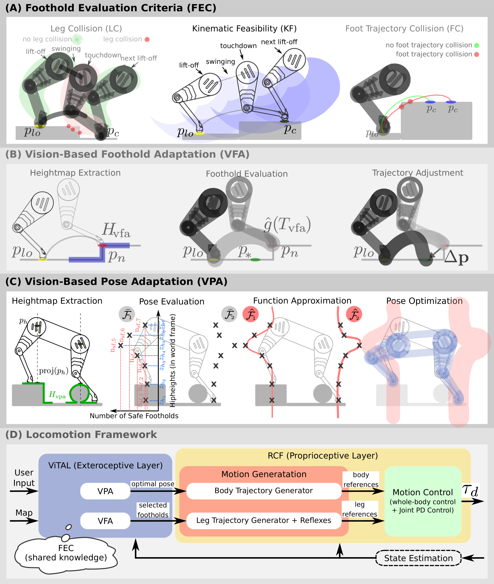
An overview of the criteria used in this work is shown in Fig. 2(A) and is detailed below.

Terrain Roughness (TR). This criterion checks edges or corners in the heightmap that are unsafe for the robot to step on. For each candidate foothold $p_{c}$ in $H$, we evaluate the mean and standard deviation of the slope relative to its neighboring footholds, and put a threshold that defines whether a $p_{c}$ is safe or not. Footholds above this threshold are discarded.

Leg Collision (LC). This criterion selects footholds that do not result in leg collision with the terrain during the entire gait cycle (from lift-off, during swinging, touchdown and till the next lift-off). To do so, we create a bounding region around the leg configuration that corresponds to the candidate foothold $p_{c}$ and the current hip location. Then, we check if the bounding region collides with the terrain (the heightmap) by measuring the closest distance between them. If this distance is lower than a certain value, then the candidate foothold is discarded.

Kinematic Feasibility (KF). This criterion selects footholds that are kinematically feasible. It checks whether a candidate foothold $p_{c}$ will result in a trajectory that remains within the workspace of the leg during the entire gait cycle. To do so, we check if the candidate foothold $p_{c}$ is within the workspace of the leg during touchdown and next lift-off. Also, we check if the trajectory of the foot from the lift-off position $p_{lo}$ till the touchdown position at the candidate foothold $p_{c}$ is within the workspace of the leg. In the initial implementation in [38], this criterion was only evaluated during touchdown. In this work, we consider this criterion during the entire leg step-cycle.

Foot Trajectory Collision (FC). This criterion selects footholds that do not result in foot trajectory collision with the terrain. It checks whether the foot swing trajectory corresponding to a candidate foothold $p_{c}$ is going to collide with the terrain or not. If the swing trajectory collides with the terrain, the candidate foothold $p_{c}$ is discarded.

Remark 1

There are three main sources of uncertainty that can affect the foothold placement [45]. These sources of uncertainty are due to trajectory tracking errors, foothold prediction errors, and drifts in the map. To allow for a degree of uncertainty, after computing $\mu_{\mathrm{safe}}$, candidate footholds that are within a radius of unsafe footholds are also discarded. This is similar to the erosion operation in image processing.

Remark 2

The initial implementation of the FEC in [38] only considered the heightmap $H$ as an input; the other inputs of the tuple $T$ in (1) were kept constant. This had a few disadvantages that we reported in [49] where we extended the work of [38] by considering the linear body heading velocity. In this work, we build upon that by considering the full body twist $v_{b}$ and the gait parameters $\alpha$ as expressed by $T$ in (1).

Figure 2: Overview of ViTAL. Illustrations are not to scale. (A) The Foothold Evaluation Criteria (FEC): Leg Collision (LC), Kinematic Feasibility (KF), and Foot Trajectory Collision (FC). (B) The Vision-based Foothold Adaptation (VFA) pipeline. First, we extract the heightmap $H_{\mathrm{vfa}}$ around the nominal foothold $p_{n}$. Then, we evaluate the heightmap either using the exact evaluation $g(T_{\mathrm{vfa}})$ or using the CNN as an approximation $\hat{g}(T_{\mathrm{vfa}})$. Once the optimal foothold $p_{*}$ is selected, the swing trajectory is adjusted. (C) The Vision-Based Pose Adaptation (VPA) pipeline. First, we extract the heightmap $H_{\mathrm{vpa}}$ for all the legs. The heightmaps are centered around the projection of the leg hip locations. Then, we evaluate the FEC to compute $\bar{\mathcal{F}}$ for all the hip heights of all the legs (pose evaluation). Then, we approximate a continuous function $\hat{\mathcal{F}}$ from $\bar{\mathcal{F}}$ (function approximation). The pose optimizer finds the pose that maximizes $\hat{\mathcal{F}}$ for all of the legs (pose optimization). (D) Our locomotion framework. ViTAL consists of the VPA and the VFA algorithms. Both algorithms rely on the robot skills which we denote by FEC. $\tau_{d}$ are the desired joint torques that are sent to the robot.

III Vision-Based Foothold Adaptation (VFA)

The VFA evaluates the FEC to select the optimal foothold for each leg [45, 38, 49]. The VFA has three main stages as shown in Fig. 2(B): heightmap extraction, foothold evaluation, and trajectory adjustment.

Heightmap Extraction. Using the current robot states and gait parameters, we estimate the touchdown position of the swinging foot in the world frame as detailed in [38]. This is denoted as the nominal foothold $p_{n}\in\mathbb{R}^{3}$. Then, we extract a heightmap $H_{\mathrm{vfa}}$ that is centered around $p_{n}$.

Foothold Evaluation. After extracting the heightmap, we compute the optimal foothold $p_{*}\in\mathbb{R}^{3}$ for each leg. We denote this by foothold evaluation which is the mapping

$$g(T_{\mathrm{vfa}}):T_{\mathrm{vfa}}\rightarrow p_{*}$$ (3)

that takes an input tuple $T_{\mathrm{vfa}}$ that is defined as

$$T_{\mathrm{vfa}}=(H_{\mathrm{vfa}},z_{h},v_{b},\alpha,p_{n}).$$ (4)

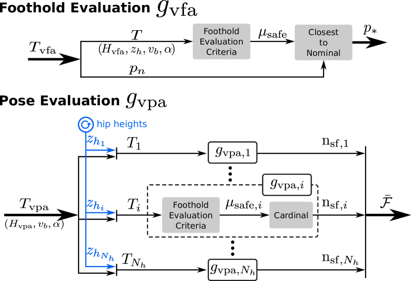
Once we evaluate the FEC in (2), from all of the safe candidate footholds in $\mu_{\mathrm{safe}}$, we select the optimal foothold $p_{*}$ as the one that is closest to the nominal foothold $p_{n}$. The aim is to minimize the deviation from the original trajectory and thus results in a less disturbed or aggressive motion. An overview of the foothold evaluation stage is shown in Fig. 3 where the tuple $T$ of the FEC in (1) is extracted from the VFA tuple $T_{\mathrm{vfa}}$ in (4) to compute $\mu_{\mathrm{safe}}$. Then, using $p_{n}$ and $\mu_{\mathrm{safe}}$, we extract $p_{*}$ as the safe foothold that is closest to $p_{n}$.

Trajectory Adjustment. The leg’s swinging trajectory is adjusted once $p_{*}$ is computed.

Figure 3: Overview of the foothold evaluation stage in the VFA algorithm, and the pose evaluation stage in the VPA algorithm.

Remark 3

To compute the foothold evaluation, one can directly apply the exact mapping $g(T_{\mathrm{vfa}})$. Yet, computing the foothold evaluation leads to evaluating the FEC which is generally computationally expensive. Thus, to speed up the computation and to continuously run the VFA online, we train a CNN to approximate the foothold evaluation $\hat{g}(T_{\mathrm{vfa}})$ using supervised learning. Once trained, the VFA can then be executed online using the CNN. The CNN architecture of the foothold evaluation is explained in Appendix -A.

IV Vision-Based Pose Adaptation (VPA)

The VPA generates pose references that maximize the chances of the legs to reach safe footholds. This means that the robot pose has to be aware of what the legs are capable of and adapt accordingly. Therefore, the goal of the VPA is to adapt the robot pose based on the same set of skills in the FEC used by the VFA.

IV-A Definitions and Notations

Number of Safe Footholds. As explained earlier, the FEC takes a tuple $T$ as an input and outputs the matrix $\mu_{\mathrm{safe}}$. Based on that, let us define the Number of Safe Footholds ($\mathrm{n_{sf}}$)

$$\mathrm{n}_{\mathrm{sf}}:=\mathrm{cardinal}(\{e\in\mu_{\mathrm{safe}}:e=1\})$$ (5)

as the number of true elements in the boolean matrix $\mu_{\mathrm{safe}}$.

Set of Safe Footholds. Consider a set of tuples $\mathcal{T}$ where each element $T_{i}\in\mathcal{T}$ is a tuple defined as

$$T_{i}=(H,z_{h_{i}},v_{b},\alpha)$$ (6)

and $z_{h_{i}}\in\mathcal{Z}$ is a hip height element in the set of hip heights $\mathcal{Z}$ (in the world frame). All the tuple elements $T_{i}\in\mathcal{T}$ share the same heightmap $H$, body twist $v_{b}$ and gait parameters $\alpha$.

Evaluating the FEC in (2) for every $T_{i}\in\mathcal{T}$ that corresponds to $z_{h_{i}}\in\mathcal{Z}$, and computing the cardinal in (5) yields $\mathrm{n}_{\mathrm{sf},i}$ for every $T_{i}$. This yields the Set of Safe Footholds ($\mathcal{F}$) which is a set containing the number of safe footholds $\mathrm{n}_{\mathrm{sf}}$ that are evaluated based on the FEC given the set of tuples $\mathcal{T}$ that corresponds to the set of hip heights $\mathcal{Z}$ but shares the same heightmap $H$, body twist $v_{b}$ and gait parameters $\alpha$.

IV-B From the Set of Safe Footholds to Pose Evaluation

The set of safe footholds $\mathcal{F}$ is one of the building blocks of the VPA. To compute $\mathcal{F}$, we compute the input tuple $T_{\mathrm{vpa}}$

$$T_{\mathrm{vpa}}=(H_{\mathrm{vpa}},v_{b},\alpha)$$ (7)

that we then augment with the hip heights $z_{h_{i}}$ in the hip heights set $\mathcal{Z}$ yielding the set of tuples $\mathcal{T}$. Then, we evaluate the FEC in (2) for every $T_{i}\in\mathcal{T}$, and computing the cardinal in (5). This can be expressed by the mapping

$${g_{\mathrm{vpa}}(T_{\mathrm{vpa}})~{}:~{}T_{\mathrm{vpa}}\rightarrow\mathcal{F}}$$ (8)

which is referred to as pose evaluation. We can express $\mathcal{F}$ as

$$\mathcal{F}=\{\mathrm{n}_{\mathrm{sf},i}=g_{\mathrm{vpa},i}(T_{i})~{}\forall T_{i}\in\mathcal{T}\}.$$ (9)

Remark 4

Since $\mathcal{Z}$ is an infinite continuous set, so is $\mathcal{F}$ which is not numerically feasible to compute. Hence, we sample a finite set $\bar{\mathcal{Z}}$ of $N_{z_{h}}$ samples of hip heights that results in a finite set of safe footholds $\bar{\mathcal{F}}$. To use the set of safe footholds in an optimization problem, we need a continuous function. Thus, after we compute $\bar{\mathcal{F}}$, we estimate a continuous function $\hat{\mathcal{F}}$ as explained next.

An overview of the pose evaluation is shown in Fig. 3 where the tuple $T_{\mathrm{vpa}}$ in (7) is augmented with the hip heights $z_{h_{i}}$ from $\bar{\mathcal{Z}}$ to construct the FEC tuples $T_{i}$ in (6). For every tuple $T_{i}$, we evaluate the FEC using (2) and compute $\mathrm{n}_{\mathrm{sf},i}$ in (5) using the mapping in (8). Finally, the set $\bar{\mathcal{F}}$ includes all the elements $\mathrm{n}_{\mathrm{sf},i}$ as in (9).

IV-C Vision-based Pose Adaptation (VPA) Formulation

The VPA has four main stages as shown in Fig. 2(C). First, heightmap extraction that is similar to the VFA. Second, pose evaluation where we compute $\bar{\mathcal{F}}$. Third, function approximation where we estimate $\hat{\mathcal{F}}$ from $\bar{\mathcal{F}}$. Fourth, pose optimization where the optimal body pose is computed.

Heightmap Extraction. We extract one heightmap $H_{\mathrm{vpa}}$ per leg that is centered around the projection of the leg’s hip location in the terrain map ($\mathrm{proj.}(p_{h})$ instead of $p_{n}$).

Pose Evaluation. After extracting the heightmaps, we compute $\bar{\mathcal{F}}$ from the mapping in (8) of the pose evaluation. In the pose evaluation, the FEC are evaluated for all hip heights in $\bar{\mathcal{Z}}$ given the input tuple $T_{\mathrm{vpa}}$ as shown in Fig. 3.

Function Approximation. In this stage, we estimate the continuous function $\hat{\mathcal{F}}$ from $\bar{\mathcal{F}}$, as explained in Remark 4. This is done by training a parameterized model of the inputs $T_{i}\in\bar{\mathcal{T}}$ and the outputs $\mathrm{n}_{\mathrm{sf},i}\in\bar{\mathcal{F}}$. The result is the function (model) $\hat{\mathcal{F}}$ that is parameterized by the model parameters $w$. The function approximation is detailed later in this section.

Pose Optimization. Evaluating the FEC and approximating it with the function $\hat{\mathcal{F}}$, introduces a metric that represents the possible number of safe footholds for every leg. Based on this, the goal of the pose optimizer is to find the optimal pose that will maximize the number of safe footholds for every leg (maximize $\hat{\mathcal{F}}$) while ensuring robustness. The pose optimizer is detailed later in this section.

Remark 5

Similar to Remark 3, one can directly apply the exact evaluation $g_{\mathrm{vpa}}(T_{\mathrm{vpa}})$ for a given $T_{\mathrm{vpa}}$. Yet, since this is computationally expensive, we rely on approximating the evaluation $\hat{g}_{\mathrm{vpa}}(T_{\mathrm{vpa}})$ using a CNN. In fact, the learning part is applied to both the pose evaluation and the function approximation. This means that the pose optimization is running online, outside the CNN. The CNN architecture of the pose evaluation is explained in Appendix -A.

IV-D Function Approximation

The goal of the function approximation is to approximate the set of safe footholds $\mathcal{F}$ from the discrete set $\bar{\mathcal{F}}$ computed in the pose evaluation stage. This is done to provide the pose optimizer with a continuous function. Given a dataset $(\bar{\mathcal{Z}},\bar{\mathcal{F}})$ of hip heights $z_{h_{i}}\in\bar{\mathcal{Z}}$ and number of safe footholds ${\mathrm{n}_{\mathrm{sf},i}\in\bar{\mathcal{Z}}}$, the function approximation estimates a function $\hat{\mathcal{F}}(z_{h_{i}},w)$ that is parameterized by the weights $w$. Once the weights $w$ are computed, the function estimate $\hat{\mathcal{F}}(z_{h_{i}},w)$ is then reconstructed and sent to the pose optimizer.

It is important to choose a function $\hat{\mathcal{F}}$ that can accurately represent the nature of the number of safe footholds. The number of safe footholds approaches zero when the hip heights approach $0$ or $\infty$. Thus, we want a function that fades to zero at the extremes (Gaussian-like functions), and captures any asymmetry or flatness in the distribution. Hence, we use radial basis functions of Gaussians. With that in mind, we are looking for the weights $w$

$$w=\text{arg}~{}\text{min}~{}S(w)$$ (10)

that minimize the cost $S(w)$

$$S(w)=\sum_{i=1}^{N_{h}}(\mathrm{n}_{\mathrm{sf},i}-\hat{\mathcal{F}}(z_{h_{i}},w))^{2}$$ (11)

which is the sum of the squared residuals of $\mathrm{n}_{\mathrm{sf},i}$ and $\hat{\mathcal{F}}(z_{h_{i}},w)$. $N_{h}$ is the number of samples (the number of the finite set of hip heights). The function $\hat{\mathcal{F}}(z_{h_{i}},w)$ is the regression model (the approximation of $\mathcal{F}$) that is parameterized by $w$. The function $\hat{\mathcal{F}}(z_{h_{i}},w)$ is the weighted sum of the basis functions

$$\hat{\mathcal{F}}(z_{h_{i}},w)=\sum_{e=1}^{E}w_{e}\cdot g(z_{h_{i}},\Sigma_{e},c_{e})$$ (12)

where $w\in\mathbb{R}^{E}$, and $E$ is the number of basis functions. The basis function is a radial basis function of Gaussian functions

$$g(z_{h_{i}},\Sigma_{e},c_{e})=\text{exp}(-0.5(z_{h_{i}}-c_{e})^{T}\Sigma_{e}^{-1}(z_{h_{i}}-c_{e}))$$ (13)

where $\Sigma_{e}$ and $c_{e}$ are the parameters of the Gaussian function. Since the function model in (12) is linear in the parameters, the weights of the function approximation can be solved analytically using least squares. In this work, we keep the parameters of the Gaussians ($\Sigma$ and $c$) fixed. Hence, the function $\hat{\mathcal{F}}$ is only parameterized by $w$. For more information on regression with radial basis functions, please refer to [57] and Appendix -B.

IV-E Pose Optimization

The pose optimizer finds the robot’s body pose $u$ that maximizes the number of safe footholds for all the legs. This is casted as a non-linear optimization problem. The notion of safe footholds is provided by the function $\hat{\mathcal{F}}(z_{h},w)$ that maps a hip height $z_{h}$ to a number of safe foothold $\mathrm{n_{sf}}$, and is parameterized by $w$. Since the pose optimizer is solving for the body pose $u$, the function $\hat{\mathcal{F}}(z_{h})$ should be encoded using the body pose rather than the hip heights (${\hat{\mathcal{F}}=\hat{\mathcal{F}}(z_{h}(u))}$). This is done by estimating the hip height as a function of the body pose (${z_{h}=z_{h}(u)}$) as shown in Appendix -C.

IV-F Single-Horizon Pose Optimization

The pose optimization problem is formulated as

$$\underset{u=[z_{b},\beta,\gamma]}{\text{maximize~{}}} \mathcal{C}(\hat{\mathcal{F}}_{l}(z_{h_{l}}(z_{b},\beta,\gamma)))~{}~{}\forall l\in N_{l}$$ (14)

subject to $$u_{\min}\leq u\leq u_{\max}$$ (15)

$$\Delta u_{\min}\leq\Delta u\leq\Delta u_{\max}$$ (16)

where $u=[z_{b},\beta,\gamma]\in\mathbb{R}^{3}$ are the decision variables (robot body pose) consisting of the robot height, roll and pitch, respectively, $\mathcal{C}$ is the cost function, $\hat{\mathcal{F}}_{l}$ is $\hat{\mathcal{F}}$ for every leg $l$ where $N_{l}=4$ is the number of legs, $z_{h_{l}}\in\mathbb{R}$ is the hip height of the leg $l$, and $u_{\min}$ and $u_{\max}$ are the lower and upper bounds of the decision variables, respectively. $\Delta u=u-u_{k-1}$ is the numerical difference of $u$ where $u_{k-1}$ is the output of $u$ at the previous instant, and $\Delta u_{\min}$ and $\Delta u_{\max}$ are the lower and upper bounds of $\Delta u$, respectively. We can re-write (16) as

$$\Delta u_{\min}+u_{k-1}\leq u\leq\Delta u_{\max}+u_{k-1}.$$ (17)

The cost function in (14) maximizes $\hat{\mathcal{F}}$ for all of the legs. We designed several types of cost functions as detailed next. The constraints in (15) and (16) ensure that the decision variables and their variations are bounded.

IV-G Cost Functions

A standard cost function can be the sum of the squares of $\hat{\mathcal{F}}_{l}$ for all of the legs

$$\mathcal{C}_{\mathrm{sum}}=\sum_{l=1}^{N_{l}=4}\|\hat{\mathcal{F}}_{l}(z_{h_{l}})\|^{2}_{Q}$$ (18)

where another option could be the product of the squares of $\hat{\mathcal{F}}_{l}$ for all of the legs

$$\mathcal{C}_{\mathrm{prod}}=\prod_{l=1}^{N_{l}=4}\|\hat{\mathcal{F}}_{l}(z_{h_{l}})\|^{2}_{Q}.$$ (19)

The key difference between an additive cost $\mathcal{C}_{\mathrm{sum}}$ and a multiplicative cost $\mathcal{C}_{\mathrm{prod}}$ is that the latter puts equal weighting for each $\hat{\mathcal{F}}_{l}$. This is important since we do not want the optimizer to find a pose that maximizes $\hat{\mathcal{F}}$ for one leg while compromising the other leg(s). One can also define the cost

$$\mathcal{C}_{\mathrm{int}}=\sum_{l=1}^{N_{l}=4}\|\int_{z_{h_{l}}-m}^{z_{h_{l}}+m}\hat{\mathcal{F}}_{l}(z_{h_{l}})~{}dz_{h_{l}}~{}\|^{2}_{Q}$$ (20)

which is the sum of squared integrals that can be numerically approximated as

$$\int_{z_{h_{l}}-m}^{z_{h_{l}}+m}\hat{\mathcal{F}}_{l}(z_{h_{l}})~{}dz_{h_{l}}\approx m\cdot(\hat{\mathcal{F}}_{l}(z_{h_{l}}-m)+\hat{\mathcal{F}}_{l}(z_{h_{l}}+m))$$ (21)

yielding

$$\mathcal{C}_{\mathrm{int}}=\sum_{l=1}^{N_{l}=4}\|m\cdot(\hat{\mathcal{F}}_{l}(z_{h_{l}}-m)+\hat{\mathcal{F}}_{l}(z_{h_{l}}+m))\|^{2}_{Q}.$$ (22)

In this cost option, we do not find the pose that maximizes $\hat{\mathcal{F}}$. Instead, we want to find the pose that maximizes the area around $\hat{\mathcal{F}}$ that is defined by the margin $m$. Using $\mathcal{C}_{\mathrm{int}}$ is important since it adds robustness in case there is any error in the pose tracking during execution. Because of possible tracking errors during execution, the robot might end up in the pose $u^{*}\pm m$ instead of $u^{*}$. If we use $\mathcal{C}_{\mathrm{int}}$ as a cost function, the optimizer will find poses that maximizes the number of safe footholds not just for $u^{*}$ but within a vicinity of $m$. More details on the use of $\mathcal{C}_{\mathrm{int}}$ as a cost function in the pose optimization of the VPA can be found in Appendix -D.

IV-H Receding-Horizon Pose Optimization

Adapting the robot’s pose during dynamic locomotion requires reasoning about what is ahead of the robot: the robot should not just consider its current state but also future ones. For that, we extend the pose optimizer to consider the current and future states of the robot in a receding horizon manner. To formulate the receding horizon pose optimizer, instead of considering $\hat{\mathcal{F}}_{l}~{}\forall~{}{l\in N_{l}}$ in the single horizon case, the pose optimizer will consider $\hat{\mathcal{F}}_{l,j}~{}\forall~{}{l\in N_{l}},~{}{j\in N_{h}}$ where $N_{h}$ is the receding horizon number. We compute $\hat{\mathcal{F}}_{l,j}$ in the same way explained in the pose evaluation stage. More details on computing $\hat{\mathcal{F}}_{l,j}$ can be found in Appendix -E.

The receding horizon pose optimization problem is

$$\underset{u=[u_{1}^{T},\cdots,u_{N_{h}}^{T}]}{\text{maximize}} \sum_{j=1}^{N_{h}}\mathcal{C}_{j}(\hat{\mathcal{F}}_{l,j}(z_{h_{l,j}}(u_{j})))$$ (23)

$$+ \sum_{j=1}^{N_{h}-1}\|u_{j}-u_{j+1}\|$$

$$\forall l\in N_{l},~{}j\in N_{h}$$

subject to $$u_{\min}\leq u\leq u_{\max}$$ (24)

$$\Delta u_{\min}\leq\Delta u\leq\Delta u_{\max}$$ (25)

where $u=[u_{1}^{T},\cdots,u_{j}^{T},\cdots,u_{N_{h}}^{T}]\in\mathbb{R}^{3N_{h}}$ are the decision variables during the entire receding horizon $N_{h}$. Each variable $u_{j}=[z_{b,j},\beta_{j},\gamma_{j}]\in\mathbb{R}^{3}$ is the optimal pose of the horizon $j$.

The first term in (23) is the sum of the cost functions $\mathcal{C}_{j}$ during the entire horizon ($\forall j\in N_{h}$). The cost $\mathcal{C}_{j}$ can be any of the aforementioned cost functions. The second term in (23) penalizes the deviation between two consecutive optimal poses within the receding horizon ($u_{j}$ and $u_{j+1}$). The second term is added so that each optimal pose $u_{j}$ is also taking into account the optimal pose of the upcoming sequence $u_{j+1}$ (to connect the solutions in a smooth way). Similar to the single horizon pose optimizer, $u_{\min}$ and $u_{\max}$ are the lower and upper bounds of the decision variables, respectively. Furthermore, $\Delta u$ denotes the numerical difference of $u$, while $\Delta u_{\min}$ and $\Delta u_{\max}$ are the lower and upper bounds of $\Delta u$, respectively. Note that the constraints of the single horizon and the receding horizon are of different dimensions.

V System Overview

Our locomotion framework that is shown in Fig. 2(D) is based on the Reactive Controller Framework (RCF) [56]. ViTAL complements the RCF with an exteroceptive terrain-aware layer composed of the VFA and the VPA. ViTAL takes the robot states, the terrain map and user commands as inputs, and sends out the selected footholds and body pose to the RCF (perceptive) layer. The RCF takes the robot states and the references from ViTAL, and uses them inside a motion generation and a motion control block. The motion generation block generates the trajectories of the leg and the body, and adjusts them with the reflexes from [56, 58]. The legs and body references from the motion generation block are sent to the motion control block. The motion control block consists of a Whole-Body Controller (WBC) [59] that generates desired torques that are tracked via a low-level torque controller [60], and sent to the robot’s joints. The framework also includes a state estimation block that feeds back the robot states to each of the aforementioned layers [61]. More implementation details on ViTAL and the entire framework is in Appendix -F.

We demonstrate ViTAL on the 90 kg HyQ and the 140 kg HyQReal quadruped robots. Each leg of the two robots has 3 degrees of freedom (3 actuated joints). The torques and angles of the 12 joints of both robots are directly measured. The bodies of HyQ and HyQReal have a tactical-grade Inertial Measurement Unit (IMU) (KVH 1775). More information on HyQ and HyQReal can be found in [62], and [3] respectively.

We noticed a significant drift in the states of the robots in experiment. To tackle this issue, the state estimator fused the data from a motion capture system and the IMU. This reduced the drift in the base states of the robots albeit not eliminating it completely. Improving the state estimation is an ongoing work and is out of the scope of this article. We used the grid map interface [63] to get the terrain map in simulation. Due to the issues with state estimation on the real robots, we constructed the grid map before the experiments, and used the motion capture system to locate the map with respect to the robot.

VI Results

We evaluate ViTAL on HyQ and HyQReal. We consider all the FEC mentioned earlier for the VFA and the VPA. We use the receding horizon pose optimizer of (25) and the sum of squared integral of (22). We choose stair climbing as an application for ViTAL. Climbing stairs is challenging for HyQ due to its limited leg workspace in the sagittal plane. Videos associated with the upcoming results can be found in the supplementary materials and [64]. Finally, an analysis of the accuracy of the CNNs and the computational time of ViTAL can be found in Appendix -G and Appendix -H, respectively.

VI-A Climbing Stairs (Simulation)

Figure 4: HyQ climbing stairs in simulation. (A) The full scenario. (B) The robot pitches up to allow for safe footholds for the front legs. (C) The robot lifts up the hind hips to avoid hind leg collisions with the step. (D) The robot pitches down to allow for safe footholds for the front legs. (E) The robot lowers the hind hips to allow for safe footholds for the legs when stepping down.

Figure 5: Climbing Stairs: A More Complex Scenario. Top: Overlayed screenshots of HyQ climbing stairs. Bottom: the optimal height and corresponding pitch (presented by the arrows) and the foot trajectories of LF and RH legs.

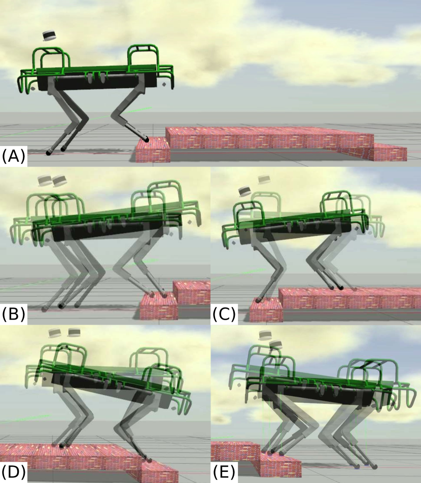
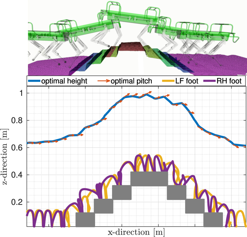
We carried out multiple simulations where HyQ is climbing the stairs shown in Fig. 4. Each step has a rise of 10 cm, and a go of 25 cm. HyQ is commanded to trot with a desired forward velocity of 0.2 m/s using the VPA and the VFA. Figure 4 shows screenshots of one simulation run, and Video 1 shows three simulation runs.

Figure 4 shows the ability of the VPA in adapting the robot pose to increase the chances of the legs to succeed in finding a safe foothold. In Fig. 4(B), HyQ raised its body and pitched upwards so that the front hips are raised to increase the workspace of the front legs when stepping up. In Fig. 4(C), HyQ raised its body and pitched downwards so that the hind hips are raised. This is done for two reasons. First, to have a larger clearance between the hind legs and the obstacle, and thus avoiding leg collision with the edge of the stairs. Second, to increase the workspace of the hind legs when stepping up, and thus avoiding reaching the workspace limits and collisions along the foot swing trajectory. In Fig. 4(D), HyQ lowered its body and pitched downwards so that the front hips are lowered. This is done for two reasons: First, to increase the workspace of the front legs when stepping down, and thus avoiding reaching the workspace limits. Second, to have a larger clearance between the front legs and the obstacle, and thus avoiding leg collisions. In Fig. 4(E), HyQ lowered its hind hips to increase the hind legs’ workspace when stepping down.

Throughout these simulations, the robot continuously adapted its body pose and its feet to find the best trade-off between increasing the kinematic feasibility, and avoiding trajectory and leg collision. This can be seen in Video 1 where the robot’s legs and the corresponding feet trajectories never collided with the terrain. The robot took multiple steps around the same foot location before stepping over an obstacle. The reason behind this is that the robot waited for the VPA to change the pose and allow for safe footholds, and then the VFA took the decision of stepping over the obstacle.

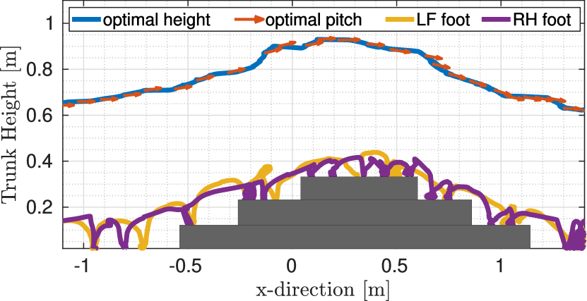
We carried out another scenario where HyQ is climbing the stairs setup in Fig. 5 where each step has a rise of 10 cm, and a go of 25 cm. HyQ is commanded to trot with a desired forward velocity of $0.2$m/s using ViTAL. The results are reported in Fig. 5 and Video 2. Figure 5 shows the robot’s height and pitch based on the VPA, and the corresponding feet trajectories of the LF leg and the RH leg based on the VFA. HyQ’s behavior was similar to the previous section: it accomplished the task without collisions or reaching workspace limits.

VI-B Climbing Stairs (Experiments)

Figure 6: HyQ and HyQReal climbing stairs in experiment. (A-F) HyQ crawling over with 0.1 m/s commanded forward velocity. (G-L) HyQ trotting over with 0.25 m/s commanded forward velocity. (M-R) HyQReal crawling over with 0.2 m/s commanded forward velocity.

Figure 7: HyQ climbing stairs in experiment. The figure shows the optimal height and corresponding pitch (presented by the arrows) based on the VPA, and the foot trajectories of the LF and RH legs based on the VFA.

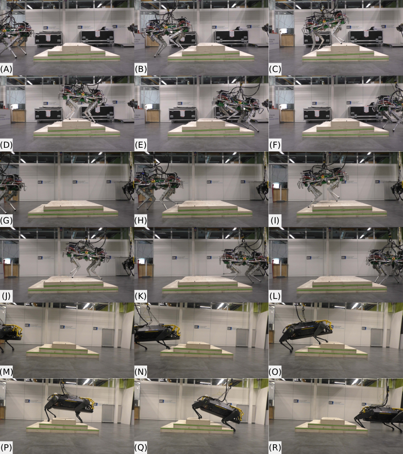
To validate ViTAL in experiments, we created three sets of experiments using the setups shown in Fig. 1. Each step has a rise of 10 cm, and a go of 28 cm.

In the first set of experiments, HyQ is commanded to crawl over the setups in Fig. 1(A,B) with a desired forward velocity of 0.1 m/s using the VPA and the VFA. Figures 6(A-F) show screenshots of one trial. Video 3 shows HyQ climbing back and forth the setup in Fig. 1(B) five times. Video 4 shows HyQ climbing the Fig. 1(A) setup, which is reported in Fig. 7. Figure 7 shows the robot’s height and pitch based on the VPA, and the corresponding feet trajectories of the Left-Front (LF) leg and the Right-Hind (RH) leg based on the VFA. This set of experiments confirms that ViTAL is effective on the real platform. The robot managed to accomplish the task without collisions or reaching workspace limits.

In the second set of experiments, HyQ is commanded to trot over the setup in Fig. 1(B) with a desired forward velocity of 0.25 m/s using the VPA and the VFA. Figures 6(G-L) show separate screenshots of this trial. Video 5 shows three trials of HyQ climbing the same setup. This set of experiments shows that ViTAL can handle different gaits.

Finally, in the third set of experiments, HyQReal is commanded to crawl over the setup in Fig. 1(C) with a desired forward velocity of 0.2 m/s using the VPA and the VFA. The results are reported in Fig. 6(M-R) that show screenshots of this trial. Video 6 shows HyQReal climbing this stair setup (Fig. 1(C)). This set of experiments shows that ViTAL can work on different legged platforms.

TABLE I: Mean Absolute Tracking Errors of the Body Pitch $\beta$ and Height $z_{b}$ of HyQ & HyQReal using ViTAL in the Experiments detailed in Section VI-B and in Fig. 1.

Description	$\beta$ [deg]	$z_{b}$ [cm]
Exp. (A): HyQ crawling at 0.1 m/s	1.0	1.5
Exp. (B): HyQ trotting at 0.2 m/s	1.0	2.3
Exp. (C): HyQReal crawling at 0.2 m/s	1.0	4.2

The tracking performance of these three sets of experiments are shown in Table I. The table shows the mean absolute tracking errors of the body pitch $\beta$ and height $z_{b}$ of HyQ and HyQReal.

VI-C Climbing Stairs with Different Forward Velocities

Figure 8: HyQ’s performance using ViTAL under different commanded velocities. The top two plots show the numerical difference of the body height and pitch ($\Delta z_{b}$ and $\Delta\gamma$), and the bottom two plots show the tracking errors of the body height and pitch.

TABLE II: Mean Absolute Tracking Errors of the Body Pitch $\beta$ and Height $z_{b}$ of HyQ using ViTAL in Simulation with Different Forward Velocities as Detailed in Section VI-C and Fig. 8.

Description	$\beta$ [deg]	$z_{b}$ [cm]
Sim. (A): HyQ trotting at 0.2 m/s	0.7	0.3
Sim. (B): HyQ trotting at 0.3 m/s	1.1	0.7
Sim. (C): HyQ trotting at 0.4 m/s	2.3	2.6
Sim. (D): HyQ trotting at 0.5 m/s	1.6	3.8

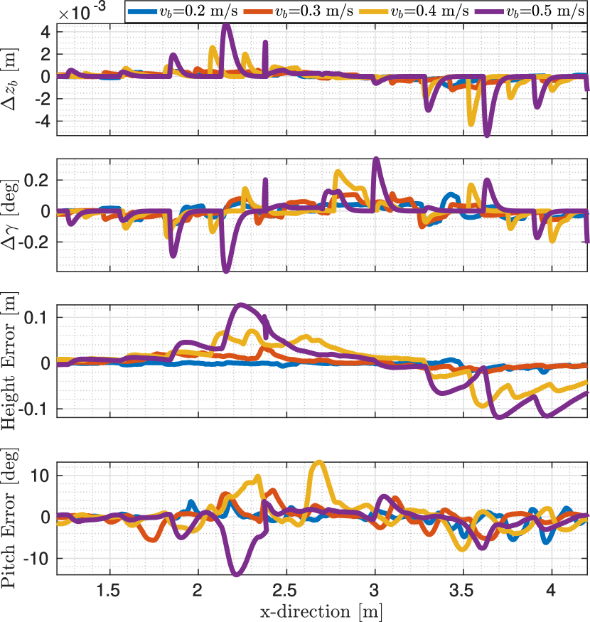
We evaluate the performance of HyQ under different commanded velocities using ViTAL. We carried out a series of simulations using the stairs setup shown in Fig. 5. HyQ is commanded to trot at four different forward velocities: 0.2 m/s, 0.3 m/s, 0.4 m/s, and 0.5 m/s. The results are reported in Fig. 8 and in Video 7. Additionally, the tracking performance of these series of simulations at the four different forward velocities are shown in Table II. The table shows the mean absolute tracking errors of the body pitch $\beta$ and height $z_{b}$ of HyQ at the corresponding commanded forward velocity. Figure 8 shows the numerical differences $\Delta z_{b}$ and $\Delta\gamma$, and the tracking errors of the body height and pitch, respectively.

HyQ was able to climb the stairs terrain under different commanded velocities. However, as the commanded velocity increases, HyQ started having faster (abrupt) changes in the body pose as shown in the top two plots of Fig. 8. As a result, the height and pitch tracking errors increase proportionally to the commanded speed as shown in the bottom two plots of Fig. 8. This can also be seen in Table II where the mean absolute tracking errors of the pitch and height increase proportionally to the commanded speed.

Similarly to HyQ, we evaluate ViTAL on HyQReal and commanded it to trot with five different forward velocities: 0.2 m/s, 0.3 m/s, 0.4 m/s, 0.5 m/s, and 0.75 m/s. We report this simulation in Video 8 where we show that ViTAL is robot independent. Yet, since the workspace of HyQReal is larger than HyQ, this scenario was more feasible to traverse for HyQReal. Thus, HyQReal was able to reach a higher commanded velocity than the ones reported for HyQ.

VI-D Comparing the VPA with a Baseline (Experiments)

Figure 9: The difference between the VPA and the TBR in six experiments (3 each). (A) The number of safe footholds corresponding to the robot pose. (B,C) The body height and pitch tracking errors, respectively. Circles (o) and crosses (x) are successful and failed trials, respectively. Unlike the VPA, the TBR failed to climb the stairs because the TBR resulted in almost no safe footholds for the four legs to reach.

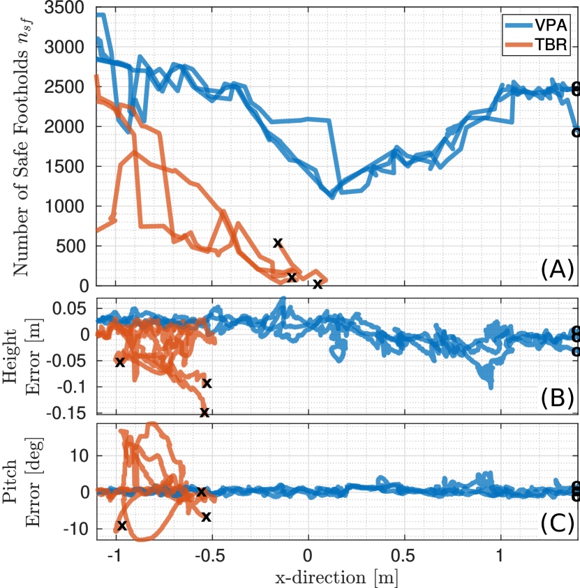
We compare the VPA with another vision-based pose adaptation strategy: the Terrain-Based Body Reference (TBR) [38]. The TBR generates pose references based on the footholds selected by the VFA. The TBR fits a plane that passes through the given selected footholds, and sets the orientation of this plane as a body orientation reference to the robot. The elevation reference of the TBR is a constant distance from the center of the approximated plane that passes through the selected footholds. We chose the TBR instead of an optimization-based strategy since the latter does not provide references that are fast enough with respect to the VPA.

Using the stairs setup in Fig. 1(A), we conducted six experimental trials: three with the VPA and three with the TBR. All trials were with the VFA. In all trials, HyQ is commanded to crawl with a desired forward velocity of 0.1 m/s. The results are reported in Fig. 9 and Video 9. Figure 9(A) shows the number of safe footholds corresponding to the robot pose from the VPA and the TBR. The robot height and pitch tracking errors are shown in Fig. 9(B,C), respectively.

As shown in Video 9, HyQ failed to climb the stairs with the TBR, while it succeeded with the VPA. This is because, unlike the VPA, the TBR does not aim to put the robot in a pose that maximizes the chances of the legs to succeed in finding safe footholds. As shown in Fig. 9(A), the number of safe footholds from using the TBR was below the ones from using the VPA. During critical periods when the robot was around 0 m in the x-direction, the number of safe footholds from using the TBR almost reached zero. The low number of safe footholds for the TBR compared to the VPA is reflected in the tracking of the robot height and pitch as shown in Fig. 9(B,C) where the tracking errors from the TBR were higher than the VPA.

The difference between the VPA and the TBR can be further explained in Video 9. When the TBR is used, the robot is adapting its pose given the selected foothold. But, if the selected foothold is not reached, or if there is a high tracking error, the robot reaches a body pose that results in a smaller number of safe footholds. Thus, the feet end up colliding with the terrain and hence the robot falls. On the other hand, the VPA is able to put the robot in a pose that maximizes the number of safe footholds. As a result, the feet found alternative safe footholds to select from, which resulted in no collision, and succeeded in climbing the stairs. The VPA optimizes for the number of safe footholds. Thus, if there is a variation around the optimal pose (tracking error), the VFA still finds more footholds to step on, which is not the case with the TBR.

VI-E Comparing the VPA with a Baseline (Simulation)

Figure 10: The difference between the VPA and the TBR in six simulations (3 each). (A) The number of safe footholds corresponding to the robot pose. (B,C) The body height and pitch tracking errors, respectively. Circles (o) and crosses (x) are successful and failed trials, respectively. Unlike the VPA, the TBR failed to climb the stairs because the TBR resulted in almost no safe footholds for the four legs to reach.

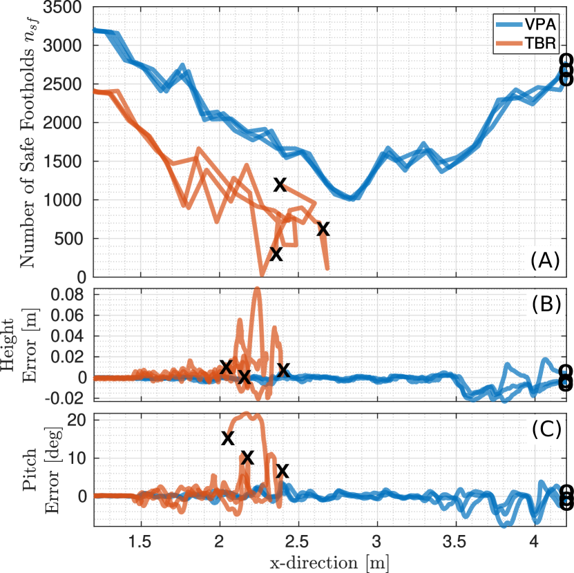
Similar to experiments, and using the stairs setup in Fig. 5, we compare the VPA with the TBR. We conducted six simulations: three with the VPA and three with the TBR. All trials were with the VFA. In all trials, HyQ is commanded to trot with a $0.2$m/s desired forward velocity. The results are reported in Fig. 10 and Video 10. Figure 10(A) shows the number of safe footholds corresponding to the robot pose from the VPA, and the TBR. The tracking errors of the robot height and pitch are shown in Fig. 10(B,C), respectively. These trials show that HyQ failed to climb the stairs using the TBR, while it succeeded using the VPA.

VI-F Climbing Stairs with Gaps

Figure 11: HyQ climbing gapped stairs. (A) Screenshots of HyQ climbing the setup. (B) The robot’s height and pitch based on the VPA, and the corresponding feet trajectories of the LF and RH legs based on the VFA. (C) The number of safe footholds using the VPA and the TBR.

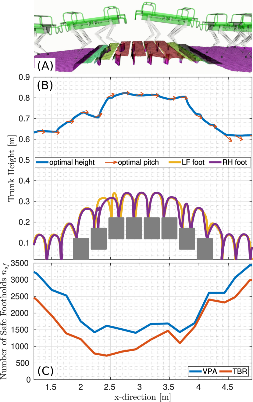
We show HyQ’s capabilities of climbing stairs with gaps using ViTAL, and we compare the VPA with the TBR. In this scenario, HyQ is commanded to trot at 0.4 m/s. Figure 11(A) shows overlayed screenshots of the simulation and the used setup. Figure 11(B) shows the robot’s height and pitch based on the VPA, and the corresponding feet trajectories of the LF leg and the RH leg based on the VFA, and Fig. 11(C) shows the number of safe footholds using the VPA and the TBR. Because of ViTAL, HyQ was able to climb the stairs with gaps while continuously adapting its pose and feet. Furthermore, the number of safe footholds from using the TBR is always lower than from using the VPA, which shows that indeed the VPA outperforms the TBR. Video 11 shows the output of this simulation using ViTAL.

VI-G Pose Optimization: Single vs. Receding Horizons

Figure 12: Pose Optimization: Single vs. Receding Horizons. (A) The number of safe footholds. (B) Variation (numerical difference) of the robot’s height. (C) Variation (numerical difference) of the robot’s pitch. (D) The tracking error of the robot’s height.

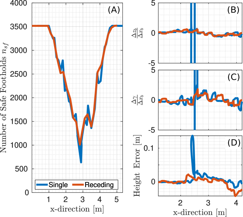
To analyze the differences between the receding horizon and the single horizon in pose optimization, we use the stairs setup in Fig. 5 with a commanded forward velocity of 0.4 m/s, and report the outcome in Fig. 12 and Video 12. The main advantage of using a receding horizon instead of a single horizon is that the pose optimization can consider future decisions. Thus, if the robot is trotting at higher velocities, the pose optimizer can adapt the robot’s pose before hand. This can result in a better adaptation strategy with less variations in the generated optimal pose. Thus, we analyze the two approaches by taking a look at the variations in the body pose

$$\acute{z}_{b}=\frac{\Delta z_{b}}{\Delta x_{b}}~{},~{}~{}~{}\text{and}~{}~{}~{}\acute{\gamma}=\frac{\Delta\gamma}{\Delta x_{b}}$$ (26)

where $\acute{z}_{b}$ and $\acute{\gamma}$ are the numerical differences (variations) of the robot height $z_{b}$ and pitch $\gamma$ with respect to the robot forward position $x_{b}$, respectively.

Figure 12 reports the differences between the two cases. The number of safe footholds is shown in Fig. 12(A). The variations in $\acute{z}_{b}$ and $\acute{\gamma}$ are shown in Fig. 12(B,C), respectively. Finally, the tracking error of the robot’s height is shown in Fig. 12(D). As shown in Figure 12 the receding horizon resulted in less variations in the body pose compared to the single horizon. This resulted in a smaller tracking error for the receding horizon in the body height, which resulted in slightly larger number of safe footholds. All in all, the receding horizon reduces variations in the desired trajectories which improves the trajectory tracking response.

The differences between the receding and single horizon in the pose optimization can also be noticed in Video 12. In the case of a single horizon, the robot was struggling while climbing up the stairs but was able to recover and accomplish the task. However, using the receding horizon, the robot was able to adapt its pose in time, and thus resulting in safer footholds that allowed the robot to accomplish the task.

Figure 13: Pose Optimization: $\mathcal{C}_{\mathrm{sum}}$ vs. $\mathcal{C}_{\mathrm{int}}$. The shaded areas are the envelopes of the number of safe footholds. The lines are the thicknesses (errors) between these envelopes.

VI-H Pose Optimization: $\mathcal{C}_{\mathrm{sum}}$ vs. $\mathcal{C}_{\mathrm{int}}$

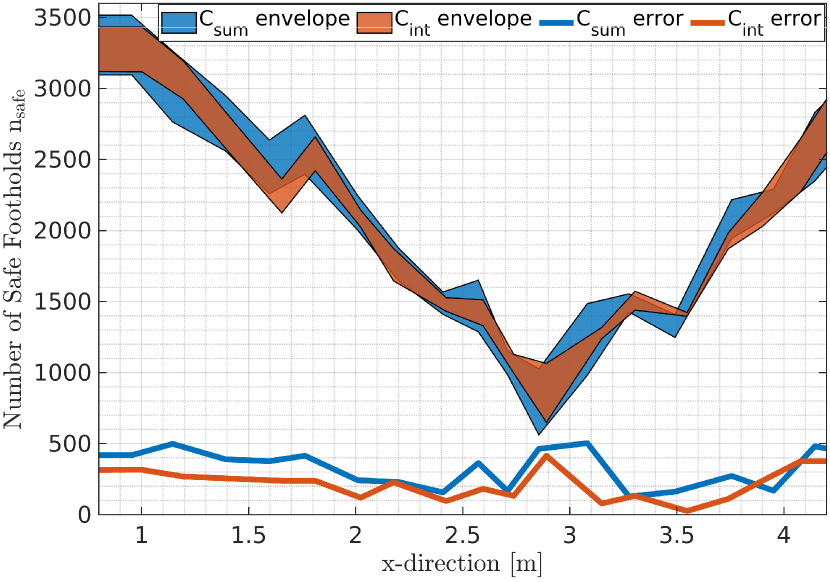
To analyze the differences between $\mathcal{C}_{\mathrm{sum}}$ and $\mathcal{C}_{\mathrm{int}}$ in the pose optimization, we use the stairs setup in Fig. 5 with a commanded forward velocity of 0.4 m/s, and report the outcome in Fig. 13. The main advantage of using $\mathcal{C}_{\mathrm{int}}$ over $\mathcal{C}_{\mathrm{sum}}$ is that $\mathcal{C}_{\mathrm{int}}$ will result in a pose that does not just maximize the number of safe footholds for all of the legs, but also ensures that the number of safe footholds of the poses around the optimal pose is still high. To compare the two cost functions, we take a look at the number of safe footholds. In particular, we evaluate the number of safe footholds corresponding to the optimal pose, and the poses around it with a margin of $m=$ 0.025 m. Thus, in Fig. 13, we plot the envelope (shaded area) between $\hat{\mathcal{F}}(u^{*}+m)$ and $\hat{\mathcal{F}}(u^{*}-m)$ for both cases, and the thickness between these envelopes which we refer to as error

$$\textbf{error}~{}=|\hat{\mathcal{F}}(u^{*}+m)-\hat{\mathcal{F}}(u^{*}-m)|.$$ (27)

As shown in Fig. 13 the envelope of the number of safe footholds resulting from $\mathcal{C}_{\mathrm{int}}$ is almost always encapsulated by $\mathcal{C}_{\mathrm{sum}}$. The thickness (error) of the number of safe footholds resulting from using $\mathcal{C}_{\mathrm{int}}$ is always smaller than $\mathcal{C}_{\mathrm{sum}}$. This means that any variation of $m$ in the optimal pose will be less critical if $\mathcal{C}_{\mathrm{int}}$ is used compared to $\mathcal{C}_{\mathrm{sum}}$.

Figure 14: HyQ traversing rough terrain and climbing stairs sideways. (A,B) HyQ traversing rough terrain with and without ViTAL, respectively. (C,D) HyQ climbing stairs while yawing (commanding the yaw rate) using ViTAL. (E,F) HyQ climbing stairs sideways using ViTAL.

VI-I Locomotion over Rough Terrain

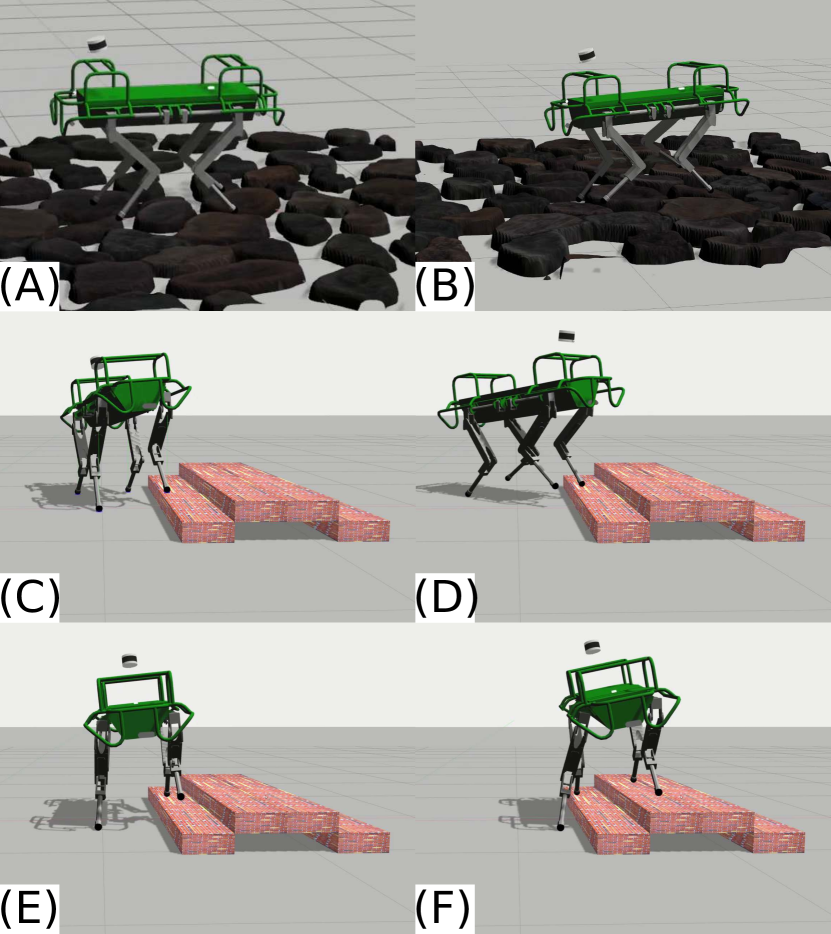
We evaluate the performance of HyQ in traversing rough terrain as shown in Fig. 14(A,B) and in Video 13. We conducted two simulations: one with ViTAL and thus with exteroceptive and proprioceptive reactions (Fig. 14(A)), and another without ViTAL and thus only with proprioceptive reactions (Fig. 14(B)). HyQ was commanded to traverse the rough terrain with a forward velocity of 0.2 m/s. No hyper parameters re-tuning, or CNNs re-training were needed.

As shown in Video 13, HyQ was able to successfully traverse the terrain in both cases. With ViTAL, HyQ collided less with the terrain and continuously adapted its footholds over the small cobblestones. Without ViTAL, HyQ traversed the rough terrain, yet, with significantly more effort. Additionally, without ViTAL, HyQ continuously collided with the terrain, and in some incidents, the feet got stuck. For this reason, we had to re-tune the gait parameters, and increase the step height to reduce these incidents. The robot’s feet also kept slipping since the feet were always close to edges and corners.

VI-J Climbing Stairs with Different Commands

Instead of commanding only forward velocities as in the previous sections, we command HyQ to climb the stairs with ViTAL while yawing (commanding the yaw rate) as shown in Video 14 and Fig. 14(C,D), and to climb stairs laterally as shown in Video 15 and Fig. 14(E,F). Climbing stairs sideways is more challenging than facing the stairs since the range of motion of the robot’s roll orientation is more restricted versus the pitch orientation. That said, because of ViTAL, HyQ was still able to climb these stairs in both cases as shown in Video 14 and Video 15.

VII Conclusion

We presented ViTAL which is an online vision-based locomotion planning strategy. ViTAL consists of the VPA for pose adaptation, and the VFA for foothold selection. The VPA introduces a different paradigm to current state-of-the-art pose adaptation strategies. The VPA finds body poses that maximize the chances of the legs to succeed in reaching safe footholds. This notion of success emerges from the robot’s skills. These skills are encapsulated in the FEC that include (but are not limited to) the terrain roughness, kinematic feasibility, leg collision, and foot trajectory collision. The VFA is a foothold selection algorithm that continuously adapts the robot’s trajectory based on the FEC. The VFA algorithm of this work extends our previous work in [49, 38] as well as the state of the art [37, 46]. Since the computation of the FEC is usually expensive, we rely on approximating these criteria with CNNs.

The robot’s skills and the notion of success provided by the FEC allowed the VPA to generate body poses that maximize the chances of success in reaching safe footholds. This resulted in body poses that are aware of the terrain and aware of what the robot and its legs can do. For that reason, the VPA was able to generate body poses that give a better chance for the VFA to select safe footholds. As a result, because of ViTAL, HyQ and HyQReal were able to traverse multiple terrains with various forward velocities and different gaits without colliding or reaching workspace limits. The terrains included stairs, gaps, and rough terrains, and the commanded velocities varied from 0.2 m/s to 0.75 m/s. The VPA outperformed other strategies for pose adaptation. We compared VPA with the TBR which is another vision based pose adaptation strategy, and showed that indeed the VPA puts the robot in a pose that provides the feet with higher number of safe footholds. Because of this, the VPA made our robots succeed in various scenarios where the TBR failed.

VIII Limitations and Future Work

One issue that we faced during experiment was in tracking the motion of the robot, especially for HyQReal. We were using a WBC for motion tracking. We believe that the motion tracking and our strategy can be improved by using a Model Predictive Control (MPC) alongside the WBC. Similarly, instead of using a model-based controller (MPC or WBC), we hypothesize that an RL-based controller can also improve the robustness and reliability of the overall robot behavior.

As explained in Section V, one other key limitation was regarding the perception system. State estimation introduced a significant drift that caused a major noise and drift in the terrain map. Albeit not being a limitation to the suggested approach, we plan on improving the state estimation and perception system of HyQ and HyQReal to allow us to test ViTAL in the wild.

The pose optimization problem of the VPA does not reason about the robot’s dynamics. This did not prevent HyQ and HyQReal from achieving dynamic locomotion while traversing challenging terrains at high speeds. However, we believe that incorporating the robot’s dynamics into ViTAL may result in a better overall performance. That said, we believe that in the future, the VPA should also reason about the robot’s dynamics. For instance, one can augment the FEC with another criterion that ensures that the selected footholds are dynamically feasible by the robot.

Additionally, in the future, we plan to extend the VPA of ViTAL to not only send pose references, but also reason about the robot’s body twist. We also plan to augment the robot skills to not only consider foothold evaluation criteria, but also skills that are tailored to the robot pose. Finally, in this work, ViTAL considered heightmaps which are 2.5D maps. In the future, we plan to consider full 3D maps that will enable ViTAL to reason about navigating in confined space (inspired by [39]).

-A CNN approximation in the VFA and the VPA

In the VFA, the foothold evaluation stage is approximated with a CNN [65] as explained in Remark 3. The CNN approximates the mapping between $T_{\mathrm{vfa}}$ and $p_{*}$. The heightmap $H_{\mathrm{vfa}}$ in $T_{\mathrm{vfa}}$ passes through three convolutional layers with $5\times 5$ kernels, $2\times 2$ padding, Leaky ReLU activation [66], and $2\times 2$ max-pooling operation. The resulted one-dimensional feature vector is concatenated with the rest of the variables in the tuple $T_{\mathrm{vfa}}$, namely, $z_{h},v_{b},\alpha,$ and $p_{n}$. This new vector passes through two fully-connected layers with Leaky ReLU and softmax activations. The parameters of the CNN are optimized to minimize the cross-entropy loss [67] of classifying a candidate foothold location as optimal $p_{*}$.

In the VPA, the pose evaluation and the function approximation is approximated with a CNN as explained in Remark 5. The CNN infers the weights $w$ of $\hat{\mathcal{F}}$ given $T_{\mathrm{vpa}}$ (the mapping between $T_{\mathrm{vpa}}$ and $w$). The heightmap $H_{\mathrm{vpa}}\in\mathbb{R}^{33\times 33}$ passes through three convolutional layers with $5\times 5$ kernels, $2\times 2$ padding, Leaky ReLU activation, and $2\times 2$ max-pooling operation. The body velocities $v_{b}$ pass through a fully-connected layer with Leaky ReLU activation that is then concatenated with the one-dimensional feature vector obtained from the heightmap. This new vector passes through two fully-connected layers with Leaky ReLU and linear activations. The parameters of this CNN are optimized to minimize the mean squared error loss between the number of safe footholds $\mathrm{n_{sf}}$ predicted by $\hat{\mathcal{F}}(z_{h},w)$ and $\hat{\mathcal{F}}(z_{h},\hat{w})$ where $\hat{w}$ are the function parameters approximated by the CNN.

For both CNNs, we used the Adam optimizer [68] with a learning rate of $0.001$, and we used a validation-based early-stopping using a $9$-to-$1$ proportion to reduce overfitting. The datasets required for training this CNNs are collected by running simulated terrain scenarios that consist of bars, gaps, stairs, and rocks. In this work, we considered a $33\times 33$ heightmap with a resolution of 0.02 m ($H_{\mathrm{vfa}},H_{\mathrm{vpa}}\in\mathbb{R}^{33\times 33}$).

Figure 15: An illustration of the Function Approximation of the VPA.

-B Details on the Function Approximation of the VPA

As explained in Section IV-D, the function $\hat{\mathcal{F}}(z_{h_{i}},w)$

$$\hat{\mathcal{F}}(z_{h_{i}},w)=\sum_{e=1}^{E}w_{e}\cdot g(z_{h_{i}},\Sigma_{e},c_{e})$$ (28)

is defined as the weighted sum of Gaussian basis functions

$$g(z_{h_{i}},\Sigma_{e},c_{e})=\text{exp}(-0.5(z_{h_{i}}-c_{e})^{T}\Sigma_{e}^{-1}(z_{h_{i}}-c_{e})).$$ (29)

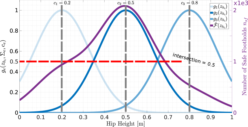
The parameters $\Sigma_{e}$ and $c_{e}$ are the widths and centers of the Gaussian function $g_{e}$ (see Section 3.1 in [57]). In the literature, $c_{e}$ is usually referred to as the mean or the expected value, and $\Sigma_{e}$ as the standard deviation. The regression algorithm should predict the weights $w_{e}$, and the parameters $\Sigma_{e}$ and $c_{e}$. To reduce the dimensionality of the problem, as explained in Section IV-D, and in Section 4.1 in [57], we decided to fix the values of the parameters of the Gaussian functions $\Sigma_{e}$ and $c_{e}$. In detail, the centers $c_{e}$ are spaced equidistantly within the bounds of the hip heights $z_{h_{i}}$, and the widths are determined by the value at which the Gaussian functions intersect. That way, the regression algorithm only outputs the weights $w_{e}$. Figure 15 shows an example of the function approximation. In this example, the bounds of the hip heights $z_{h_{i}}$ are 0.2 m and 0.8 m. Assuming a number of basis functions $E=3$, the centers $c_{e}$ are then chosen to be equidistant within the bounds, and thus, the centers $c_{e}$ are 0.2 m, 0.3 m and 0.8 m. By choosing the Gaussian functions to intersect at 0.5, the widths $\Sigma_{e}$ are 0.13.

-C Representing the Hip Heights in terms of the Body Pose

To represent the hip heights in terms of the body pose, we first write the forward kinematics of the robot’s hips

$$p_{h_{i}}^{W}=p_{b}^{W}~{}+~{}R_{b}^{W}p_{h_{i}}^{b}$$ (30)

where $p_{h_{i}}^{W}\in\mathbb{R}^{3}$ is the position of the hip of the $i$th leg in the world frame, $p_{b}^{W}\in\mathbb{R}^{3}$ is the position of the robot’s base in the world frame, $R_{b}^{W}\in SO(3)$ is the rotation matrix mapping vectors from the base frame to the world frame, and $p_{h_{i}}^{b}\in\mathbb{R}^{3}$ is the position of the hip of the $i$th leg in the base frame. The rotation matrix $R_{b}^{W}$ is a representation of the Euler angles of the robot’s base with sequence of roll $\beta$, pitch $\gamma$, and yaw $\psi$ (Cardan angles) [69]. The variable $p_{h_{i}}^{b}$ is obtained from the CAD of the robot. Expanding (30) yields

$$\begin{bmatrix}x_{h_{i}}^{W}\\ y_{h_{i}}^{W}\\ z_{h_{i}}^{W}\end{bmatrix} = \begin{bmatrix}x_{b}^{W}\\ y_{b}^{W}\\ z_{b}^{W}\end{bmatrix}+R_{b}^{w}(\beta,\gamma,\psi)\begin{bmatrix}x_{h_{i}}^{b}\\ y_{h_{i}}^{b}\\ z_{h_{i}}^{b}\end{bmatrix}$$ (31)

$$= \begin{bmatrix}x_{b}^{W}\\ y_{b}^{W}\\ z_{b}^{W}\end{bmatrix}+\begin{bmatrix}\cdots&\cdots&\cdots\\ \cdots&\cdots&\cdots\\ -s\gamma&c\gamma~{}s\beta&c\gamma~{}c\beta\end{bmatrix}\begin{bmatrix}x_{h_{i}}^{b}\\ y_{h_{i}}^{b}\\ z_{h_{i}}^{b}\end{bmatrix}$$ (32)

where $s$ and $c$ are sine and cosine of the angles, respectively. Since we are interested only in the hip heights, the z-component (third row) of (32) yields

$$z_{h_{i}}^{W}=z_{b}^{W}-x_{h_{i}}^{b}s\gamma+y_{h_{i}}^{b}c\gamma s\beta+z_{h_{i}}^{b}c\gamma c\beta.$$ (33)

-D Details on Using the Sum of Squared Integrals as a Cost Function in the Pose Optimization Problem of the VPA

Figure 16: Using the sum of squared integrals as a cost function in the pose optimization of the VPA. The two curves represent $\hat{\mathcal{F}}_{l}$. The x-axis is the hip height and the y-axis is $\mathrm{n_{sf}}$. The figure shows two optimal poses: $u_{1}^{*}$ which is from using $\mathcal{C}_{\mathrm{sum}}$ or $\mathcal{C}_{\mathrm{prod}}$, and $u_{2}^{*}$ which is from using $\mathcal{C}_{\mathrm{int}}$.

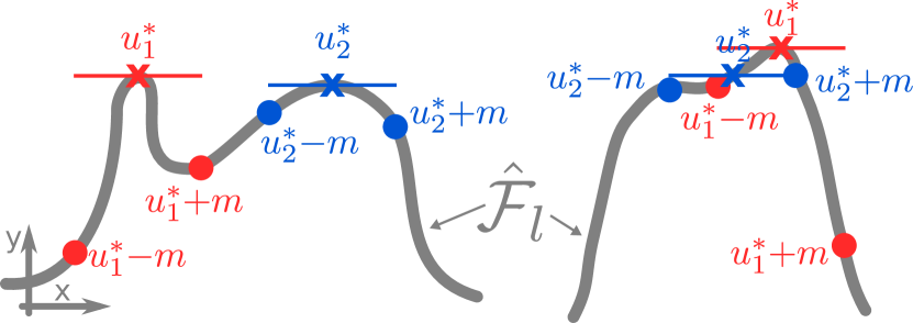
Using $\mathcal{C}_{\mathrm{int}}$ as a cost function can be motivated by taking Fig. 16 as an example. In this figure, there are two curves that represent $\hat{\mathcal{F}}_{l}$ where the horizontal axis is the hip height and the vertical axis represent $\mathrm{n_{sf}}$. The figure shows two optimal poses where $u_{1}^{*}$ is the optimal pose using the cost functions $\mathcal{C}_{\mathrm{sum}}$ or $\mathcal{C}_{\mathrm{prod}}$ that only maximize for $\hat{\mathcal{F}}_{l}$, and $u_{2}^{*}$ is the optimal pose using the cost function $\mathcal{C}_{\mathrm{int}}$. As shown in the figure, if $\mathcal{C}_{\mathrm{sum}}$ or $\mathcal{C}_{\mathrm{prod}}$ is used, the optimal pose will be $u_{1}^{*}$ which is indeed the one that results in the maximum $\hat{\mathcal{F}}_{l}$. However, if there is a tracking error of $m$ (thus the robot reaches $u_{1}^{*}\pm m$), the robot might end up in the pose $u_{1}^{*}\pm m$ that results in a small number of safe footholds. Using $\mathcal{C}_{\mathrm{int}}$ will take into account the safe footholds within a margin $m$. This might result in a pose that does not yield the maximum number of safe footholds, but it will result in a safer foothold in case the robot pose has any tracking errors. Note that using the sum of squared integrals $\mathcal{C}_{\mathrm{int}}$ as a cost function is similar to smoothing $\hat{\mathcal{F}}_{l}$ with respect to the hip height (a moving average smoothing). Using a smoothing function $\mathcal{C}_{s}$ may take the form

$$\mathcal{C}_{s}=\sum_{l=1}^{N_{l}=4}\|\frac{1}{2\epsilon}\sum_{i=-\epsilon}^{\epsilon}\hat{\mathcal{F}}_{l}(z_{h_{l}}+i)\ \|^{2}_{Q}.$$ (34)

-E Defining the Receding Horizon

In the receding horizon there is a tuple $T_{\mathrm{vpa},j}$ for every $j$th horizon that is defined as

$$T_{\mathrm{vpa},j}=(H_{\mathrm{vpa},j},v_{b},\alpha)$$ (35)

hence sharing the same body twist $v_{b}$ and gait parameters $\alpha$ but a different heightmap $H_{\mathrm{vpa},j}$. For every leg, a heightmap of horizon $j+1$ is overlapping with the previous horizon’s $j$ heightmap. This overlap has a magnitude of $\Delta h$ taking the same direction as the body velocity $\dot{x}_{b}$. Without loss of generality, we chose the magnitude of the overlap to be half of the diagonal size of the heightmap in this work. To sum up, we first gather $T_{\mathrm{vpa},j}$ that share the same $v_{b}$ and $\alpha$, but a different $H_{\mathrm{vpa},j}$. Then, we evaluate $T_{\mathrm{vpa},j}$ and approximate the output using the function approximation yielding $\hat{\mathcal{F}}_{j}$ that is sent to the optimizer for all of the legs.

-F Miscellaneous Settings

In this work, all simulations were conducted on an Intel Core i7 quad-core CPU, and all experiments were running on an onboard Intel Core i7 quad-core CPU where state estimation, mapping, and controls were running. The RCF (including the WBC) runs at 250 Hz, the low-level controller runs at 1000 Hz, the state estimator runs at 333 Hz, and the mapping algorithm runs at 20 Hz. The VPA and the VFA run asynchronously at the maximum possible update rate.

ViTAL is implemented in Python. The CNNs are implemented in PyTorch [70]. As explained in Appendix -A, in this work, we considered a $33\times 33$ heightmap with a resolution of 0.02 m ($H_{\mathrm{vfa}},H_{\mathrm{vpa}}\in\mathbb{R}^{33\times 33}$). The finite set $\bar{\mathcal{Z}}$ consisted of a hip height range between 0.2 m and 0.8 m with a resolution of 0.02 m yielding $N_{z_{h}}=31$ samples. The number of radial basis functions used in the function approximation was $E=30$. The pose optimization problem is solved with a trust-region interior point method [71, 72] which is a non-linear optimization problem solver that we solved using SciPy [73]. The bounds of the pose optimization problem $u_{\min}$ and $u_{\max}$ are $[0.2\,\mathrm{m},-0.35\,\mathrm{rad},-0.35\,\mathrm{rad}]$, and $[0.8\,\mathrm{m},0.35\,\mathrm{rad},0.35\,\mathrm{rad}]$, respectively. We used a receding horizon of $N_{h}=2$ with a map overlap of half the size of the heightmap. For a heightmap of a size of $33\times 33$ and a resolution of 0.02 m, the map overlap $\Delta h$ is 0.33 m. We used Gazebo [74] for the simulations, and ROS for communication.

-G Estimation Accuracy

We compare the estimation accuracy of the VFA by comparing the output of the foothold evaluation stage (explained in Section III) given the same input tuple $T_{\mathrm{vfa}}$. That is to say, we compare the estimation accuracy of the VFA by comparing $\hat{g}(T_{\mathrm{vfa}})$ versus $g(T_{\mathrm{vfa}})$ (see Remark 3). To do so, once trained, we generated a dataset of 4401 samples from randomly sampled heightmaps for every leg. This analysis was done on HyQ.

As explained in Section III, from all of the safe candidate footholds in $\mu_{\mathrm{safe}}$, the VFA chooses the optimal foothold to be the one closest to the nominal foothold. Thus, to fairly analyse the estimation accuracy of the VFA, we present three main measures: perfect match being the amount of samples where $\hat{g}(T_{\mathrm{vfa}})$ outputted the exact value of $g(T_{\mathrm{vfa}})$, safe footholds, being the amount of samples where $\hat{g}(T_{\mathrm{vfa}})$ did not output the exact value of $g(T_{\mathrm{vfa}})$, but rather a foothold that is safe but not closest to the nominal foothold, and mean distance, being the average distance of the estimated optimal foothold from $\hat{g}(T_{\mathrm{vfa}})$ relative to the exact foothold from $g(T_{\mathrm{vfa}})$. These measures are presented as the mean of all legs.

Based on that, the perfect match measure is $74.0\%$. Thus, $74\%$ of $\hat{g}(T_{\mathrm{vfa}})$ perfectly matched $g(T_{\mathrm{vfa}})$. The safe footholds measure is $93.7\%$. Thus, $93.7\%$ of $\hat{g}(T_{\mathrm{vfa}})$ were deemed safe. Finally, the mean distance of the estimated optimal foothold from $\hat{g}(T_{\mathrm{vfa}})$ relative to the exact foothold from $g(T_{\mathrm{vfa}})$ is 0.02 m. This means that, on average, $\hat{g}(T_{\mathrm{vfa}})$ yielded optimal footholds that are 0.02 m far from the optimal foothold from $g(T_{\mathrm{vfa}})$. Note that, the radius of HyQ’s foot, and the resolution of the heightmap is also 0.02 m, which means that the average distance measure is still acceptable especially since we account for this value in the uncertainty margin as explained in Remark 1.

Similar to the VFA, we compare the accuracy of VPA by comparing the output of the pose evaluation stage (explained in Section IV-C) given the same input tuple $T_{\mathrm{vfa}}$. That is to say, we compare the estimation accuracy of the VPA by comparing $\bar{\mathcal{F}}$ versus $\hat{\mathcal{F}}$ (see Remark 4 and Remark 5). To do so, we ran one simulation using the stairs setup shown in Fig. 5 on HyQ, and gathered the input tuple $T_{\mathrm{vfa}}$. Then, we ran the VPA offline, once with the exact evaluation (yielding $\bar{\mathcal{F}}$) and once with the approximate one (yielding $\hat{\mathcal{F}}$).

Based on this simulation run, the mean values of the exact and the approximate evaluations are $\mathrm{mean}(\bar{\mathcal{F}})=1370$ and $\mathrm{mean}(\hat{\mathcal{F}})=1322$, respectively. This yields an estimation accuracy $\mathrm{mean}(\hat{\mathcal{F}})/\mathrm{mean}(\bar{\mathcal{F}})$ of $96.5\%$.

-H Computational Analysis

To analyze the computational time of the VFA and the VPA, we ran one simulation using the stairs setup shown in Fig. 5 on HyQ to gather the input tuples of the VFA and the VPA, $T_{\mathrm{vfa}}$ and $T_{\mathrm{vpa}}$, respectively. Then, we ran both algorithms offline, once with the exact evaluation and once using the CNNs, and collected the time it took to run both algorithms (all stages included). The mean and standard deviation of the time taken to compute the exact and the CNN-approximated VFA (per leg) algorithms are $7.5\,\mathrm{ms}\pm 1\,\mathrm{ms}$, and $3.5\,\mathrm{ms}\pm 1\,\mathrm{ms}$, respectively. The mean and standard deviation of the time taken to compute the exact and the CNN-approximated VPA algorithms are $720\,\mathrm{ms}\pm 68\,\mathrm{ms}$, and $180\,\mathrm{ms}\pm 60\,\mathrm{ms}$, respectively. Hence, the VFA and the VPA can run at roughly 280 Hz and 5 Hz, respectively. This also shows that the CNNs can speed up the evaluation of the VFA and the VPA up to 4 times and 2 times, respectively.

Note that it takes longer to compute the VFA of this work versus our previous work [38]. This is because the VFA of this work considers more inputs than in our previous work, and thus, the size of the CNN is larger. As can be seen, the VPA runs at a relatively lower update rate compared to the VFA. We believe that this is not an issue since the VFA runs at the legs-level while the VPA runs as the body-level which means that the legs experience faster dynamics than the body.

During simulations and experiments, the CNNs were running on a CPU. A significant amount of computational time can be reduced if we run the CNNs of the VFA and the VPA on a GPU. Likewise, a significant amount of computational time can be reduced if a different pose optimization solver is used. However, both suggestions are beyond the scope of this work, and are left as a future work.

Glossary

CNN

Convolutional Neural Network

RL

Reinforcement Learning

FC

Foot Trajectory Collision

$\mathcal{F}$

Set of Safe Footholds

FEC

Foothold Evaluation Criteria

HyQ

Hydraulically actuated Quadruped

KF

Kinematic Feasibility

LC

Leg Collision

MPC

Model Predictive Control

$\mathrm{n_{sf}}$

Number of Safe Footholds

RCF

Reactive Controller Framework

TAL

Terrain-Aware Locomotion

TBR

Terrain-Based Body Reference

TO

Trajectory Optimization

TR

Terrain Roughness

VFA

Vision-Based Foothold Adaptation

ViTAL

Vision-Based Terrain-Aware Locomotion

VPA

Vision-Based Pose Adaptation

WBC

Whole-Body Controller

Shamel Fahmi (S’19) was born in Cairo, Egypt. He received the B.Sc. degree in Mechatronics from the German University in Cairo, Cairo, Egypt, in 2015, the M.Sc. degree in Systems and Control from the University of Twente, Enschede, the Netherlands, in 2017, and the Ph.D. degree in Advanced and Humanoid Robotics from the Italian Institute of Technology, Genoa, Italy, in 2021. His Ph.D. was on terrain-aware locomotion for legged robots. Currently, he is researcher at the Biomimetic Robotics Lab, Massachusetts Institute of Technology, MA, USA. His research interests include locomotion planning and control for quadruped and humanoid robots using model- and learning-based methods.

Victor Barasuol received the Diploma in electrical engineering from Universidade do Estado de Santa Catarina (UDESC), Joinville, Brazil, in 2006. He has a M.Sc. degree in electrical engineering and a Ph.D. degree in automation and systems engineering, both obtained from Universidade Federal de Santa Catarina (UFSC), Florianópolis, Brazil, in 2008 and 2013, respectively. He is currently a researcher at the Dynamic Legged Systems (DLS) lab at Istituto Italiano di Tecnologia (IIT), Genoa, Italy. He is knowledgeable from the kinematic design to the control of hydraulic quadruped robots, with major expertise in dynamic motion generation and control. His research activities focus on proprioceptive-based and exteroceptive-based reactions, whole-body control, machine learning for locomotion, active impedance modulation, and loco-manipulation.

Domingo Esteban received the B.Sc. degree in industrial engineering from the Universidad Nacional de San Agustin, Arequipa, Peru, in 2009, the M.Sc. degree in robotics and automation from the Universidad Carlos III, Madrid, Spain, in 2014, and the Ph.D. degree in advanced and humanoid robotics from the Italian Institute of Technology (IIT), Genoa, Italy, in 2019. From 2019 to 2021, he was a Postdoctoral Researcher with the Dynamic Legged Systems Lab at IIT. He is currently working at ANYbotics A.G., Zurich, Switzerland. He is interested in machine learning for decision-making and motion control in robotics.

Octavio Villarreal received the M.Sc. degree in mechanical engineering track control engineering from TU Delft, The Netherlands, in 2016, and the Ph.D. degree from IIT and the University of Genoa, in 2019, working at the Dynamic Legged Systems (DLS) lab for his work on vision-based foothold adaptation and locomotion strategies for legged robots. He is currently a robotics research engineer at Dyson Technology Ltd.

Claudio Semini (S’07-M’10) received the M.Sc. degree in electrical engineering and information technology from ETH, Zurich, Switzerland, in 2005, and the Ph.D. degree in humanoid technologies from Istituto Italiano di Tecnologia (IIT), Genoa, Italy, in 2010. During his doctorate, he developed the hydraulic quadruped robot HyQ and worked on its control. Since 2012, he leads the Dynamic Legged Systems (DLS) lab. He is a co-founder of the Technical Committee on Mechanisms and Design of the IEEE-RAS Society. He is/was the coordinator/partner of several EU-, National and Industrial projects (including HyQ-REAL, INAIL Teleop, Moog@IIT joint lab, ESA-ANT, etc). His research interests include the design and control of highly dynamic and versatile legged robots for real-world operations, locomotion, hydraulics, and others.

References

- [1] J. Lee, J. Hwangbo, L. Wellhausen, V. Koltun, and M. Hutter, “Learning quadrupedal locomotion over challenging terrain,” Sci. Robot., vol. 5, no. 47, p. eabc5986, Oct. 2021, DOI:10.1126/scirobotics.abc5986.
- [2] C. Yang, K. Yuan, Q. Zhu, W. Yu, and Z. Li, “Multi-expert learning of adaptive legged locomotion,” Sci. Robot., vol. 5, no. 49, p. eabb2174, Dec. 2020, DOI:10.1126/scirobotics.abb2174.
- [3] C. Semini, V. Barasuol, M. Focchi, C. Boelens, M. Emara, S. Casella, O. Villarreal, R. Orsolino, G. Fink, S. Fahmi, G. Medrano-Cerda, and D. G. Caldwell, “Brief introduction to the quadruped robot HyQReal,” in Italian Conference on Robotics and Intelligent Machines (I-RIM), Rome, Italy, Oct. 2019, pp. 1–2.
- [4] B. Katz, J. D. Carlo, and S. Kim, “Mini cheetah: A platform for pushing the limits of dynamic quadruped control,” in Proc. IEEE Int. Conf. Robot. Automat. (ICRA), Montreal, QC, Canada, May 2019, pp. 6295–6301, DOI:10.1109/ICRA.2019.8793865.
- [5] G. Bledt, M. J. Powell, B. Katz, J. Di Carlo, P. M. Wensing, and S. Kim, “MIT Cheetah 3: Design and control of a robust, dynamic quadruped robot,” in Proc. IEEE/RSJ Int. Conf. Intell. Robot. Syst. (IROS), Madrid, Spain, Oct. 2018, pp. 2245–2252, DOI:10.1109/IROS.2018.8593885.
- [6] M. Hutter, C. Gehring, D. Jud, A. Lauber, C. D. Bellicoso, V. Tsounis, J. Hwangbo, K. Bodie, P. Fankhauser, M. Bloesch, R. Diethelm, S. Bachmann, A. Melzer, and M. Hoepflinger, “Anymal - a highly mobile and dynamic quadrupedal robot,” in Proc. IEEE/RSJ Int. Conf. Intell. Robot. Syst. (IROS), Daejeon, South Korea, Oct. 2016, pp. 38–44, DOI:10.1109/IROS.2016.7758092.
- [7] Boston Dynamics, Spot, 2021, https://www.bostondynamics.com/spot, [Online; accessed Aug. 2022].
- [8] Agility Robotics, Robots, 2021, https://www.agilityrobotics.com/robots, [Online; accessed Aug. 2022].
- [9] Unitree Robotics, Go1, 2021, https://www.unitree.com/products/go1, [Online; accessed Aug. 2022].
- [10] S. Fahmi, “On terrain-aware locomotion for legged robots,” Ph.D. dissertation, Istituto Italiano di Tecnologia (IIT), Apr. 2021. [Online]. Available: https://arxiv.org/abs/2212.00683
- [11] R. Buchanan, J. Bednarek, M. Camurri, M. Nowicki, K. Walas, and M. Fallon, “Navigating by touch: haptic monte carlo localization via geometric sensing and terrain classification,” Auton. Robot., vol. 45, pp. 843–857, Aug. 2021, DOI:https://doi.org/10.1007/s10514-021-10013-w.
- [12] S. Fahmi, G. Fink, and C. Semini, “On state estimation for legged locomotion over soft terrain,” IEEE Sens. Lett. (L-SENS), vol. 5, no. 1, pp. 1–4, Jan. 2021.
- [13] S. Wang, A. Bhatia, M. T. Mason, and A. M. Johnson, “Contact localization using velocity constraints,” in Proc. IEEE/RSJ Int. Conf. Intell. Robot. Syst. (IROS), Las Vegas, NV, USA (Virtual), Oct. 2020, pp. 7351–7358.
- [14] A. Ahmadi, T. Nygaard, N. Kottege, D. Howard, and N. Hudson, “Semi-supervised gated recurrent neural networks for robotic terrain classification,” IEEE Robot. Automat. Lett. (RA-L), vol. 6, no. 2, pp. 1848–1855, Feb. 2021, DOI:10.1109/LRA.2021.3060437.
- [15] H. C. Lin and M. Mistry, “Contact surface estimation via haptic perception,” in Proc. IEEE Int. Conf. Robot. Automat. (ICRA), Paris, France (Virtual), May 2020, pp. 5087–5093, DOI:10.1109/ICRA40945.2020.9196816.
- [16] S. Fahmi, M. Focchi, A. Radulescu, G. Fink, V. Barasuol, and C. Semini, “Stance: Locomotion adaptation over soft terrain,” IEEE Trans. Robot. (T-RO), vol. 36, no. 2, pp. 443–457, Apr. 2020, DOI:10.1109/TRO.2019.2954670.
- [17] K. Paigwar, L. Krishna, S. Tirumala, N. Khetan, A. Sagi, A. Joglekar, S. Bhatnagar, A. Ghosal, B. Amrutur, and S. Kolathaya, “Robust quadrupedal locomotion on sloped terrains: A linear policy approach,” in Proc. Conf. Robot Learn. (CoRL), Virtual, Nov. 2020, pp. 1–11.
- [18] L. Wellhausen, A. Dosovitskiy, R. Ranftl, K. Walas, C. Cadena, and M. Hutter, “Where should i walk? predicting terrain properties from images via self-supervised learning,” IEEE Robot. Automat. Lett. (RA-L), vol. 4, no. 2, pp. 1509–1516, Jan. 2019, DOI:10.1109/LRA.2019.2895390.
- [19] W. Bosworth, J. Whitney, Sangbae Kim, and N. Hogan, “Robot locomotion on hard and soft ground: Measuring stability and ground properties in-situ,” in Proc. IEEE Int. Conf. Robot. Automat. (ICRA), Stockholm, Sweden, May 2016, pp. 3582–3589, DOI:10.1109/ICRA.2016.7487541.
- [20] D. D. Fan, K. Otsu, Y. Kubo, A. Dixit, J. Burdick, and A. Agha-mohammadi, “STEP: Stochastic Traversability Evaluation and Planning for Risk-Aware Off-road Navigation,” in Proc. Robot.: Sci. and Syst. (RSS), Virtual, Jul. 2021, pp. 1–12, DOI:10.15607/RSS.2021.XVII.021.
- [21] O. Melon, R. Orsolino, D. Surovik, M. Geisert, I. Havoutis, and M. Fallon, “Receding-horizon perceptive trajectory optimization for dynamic legged locomotion with learned initialization,” in Proc. IEEE Int. Conf. Robot. Automat. (ICRA), Xi’an, China (Virtual), Jun. 2021, pp. 9805–9811, DOI:10.1109/ICRA48506.2021.9560794.
- [22] B. Ponton, M. Khadiv, A. Meduri, and L. Righetti, “Efficient multicontact pattern generation with sequential convex approximations of the centroidal dynamics,” IEEE Trans. Robot. (T-RO), vol. 37, no. 5, pp. 1661–1679, Feb. 2021, DOI:10.1109/TRO.2020.3048125.
- [23] C. Mastalli, R. Budhiraja, W. Merkt, G. Saurel, B. Hammoud, M. Naveau, J. Carpentier, L. Righetti, S. Vijayakumar, and N. Mansard, “Crocoddyl: An efficient and versatile framework for multi-contact optimal control,” in Proc. IEEE Int. Conf. Robot. Automat. (ICRA), Virutal, May 2020, pp. 2536–2542, DOI:10.1109/ICRA40945.2020.9196673.
- [24] A. W. Winkler, C. D. Bellicoso, M. Hutter, and J. Buchli, “Gait and trajectory optimization for legged systems through phase-based end-effector parameterization,” IEEE Robot. Automat. Lett. (RA-L), vol. 3, no. 3, pp. 1560–1567, Feb. 2018, DOI:10.1109/LRA.2018.2798285.
- [25] C. Mastalli, I. Havoutis, M. Focchi, D. G. Caldwell, and C. Semini, “Motion planning for quadrupedal locomotion: Coupled planning, terrain mapping and whole-body control,” IEEE Trans. Robot. (T-RO), vol. 36, no. 6, pp. 1635–1648, Apr. 2020, DOI:10.1109/TRO.2020.3003464.
- [26] M. Brunner, B. Brüggemann, and D. Schulz, “Hierarchical rough terrain motion planning using an optimal sampling-based method,” in Proc. IEEE Int. Conf. Robot. Automat. (ICRA), Karlsruhe, Germany, May 2013, pp. 5539–5544, DOI:10.1109/ICRA.2013.6631372.
- [27] H. Li and P. M. Wensing, “Hybrid systems differential dynamic programming for whole-body motion planning of legged robots,” IEEE Robot. Automat. Lett. (RA-L), vol. 5, no. 4, pp. 5448–5455, Jul. 2020, DOI:10.1109/LRA.2020.3007475.
- [28] H. Li, R. J. Frei, and P. M. Wensing, “Model hierarchy predictive control of robotic systems,” IEEE Robot. Automat. Lett. (RA-L), vol. 6, no. 2, pp. 3373–3380, Feb. 2021, DOI:10.1109/LRA.2021.3061322.
- [29] N. Rudin, D. Hoeller, P. Reist, and M. Hutter, “Learning to walk in minutes using massively parallel deep reinforcement learning,” in Proc. Conf. Robot Learn. (CoRL), London, UK, Nov. 2021, pp. 91–100.
- [30] W. Yu, D. Jain, A. Escontrela, A. Iscen, , P. Xu, E. Coumans, S. Ha, J. Tan, and T. Zhang, “Visual-locomotion: Learning to walk on complex terrains with vision,” in Proc. Conf. Robot Learn. (CoRL), London, UK, Nov. 2021, pp. 1291–1302.
- [31] T. Miki, J. Lee, J. Hwangbo, L. Wellhausen, V. Koltun, and M. Hutter, “Learning robust perceptive locomotion for quadrupedal robots in the wild,” Sci. Robot., vol. 7, no. 62, p. eabk2822, Jan. 2022, DOI:10.1126/scirobotics.abk2822.
- [32] S. Gangapurwala, M. Geisert, R. Orsolino, M. Fallon, and I. Havoutis, “Real-time trajectory adaptation for quadrupedal locomotion using deep reinforcement learning,” in Proc. IEEE Int. Conf. Robot. Automat. (ICRA), Xi’an, China (Virtual), Oct. 2021, pp. 1–7.
- [33] A. Kumar, Z. Fu, D. Pathak, and J. Malik, “RMA: Rapid motor adaptation for legged robots,” in Proc. Robot.: Sci. and Syst. (RSS), Virtual, Jul. 2021, pp. 1–15, DOI:10.15607/RSS.2021.XVII.011Fe.
- [34] J. Siekmann, K. Green, J. Warila, A. Fern, and J. Hurst, “Blind bipedal stair traversal via sim-to-real reinforcement learning,” in Proc. Robot.: Sci. and Syst. (RSS), Virtual, Jul. 2021, pp. 1–9, DOI:10.15607/RSS.2021.XVII.061.
- [35] V. Tsounis, M. Alge, J. Lee, F. Farshidian, and M. Hutter, “Deepgait: Planning and control of quadrupedal gaits using deep reinforcement learning,” IEEE Robot. Automat. Lett. (RA-L), vol. 5, no. 2, pp. 3699–3706, Mar. 2020, DOI:10.1109/LRA.2020.2979660.
- [36] M. Kalakrishnan, J. Buchli, P. Pastor, M. Mistry, and S. Schaal, “Learning, planning, and control for quadruped locomotion over challenging terrain,” Int. J. Robot. Res. (IJRR), vol. 30, no. 2, pp. 236–258, Nov. 2011, DOI:10.1177/0278364910388677.
- [37] P. Fankhauser, M. Bjelonic, C. Dario Bellicoso, T. Miki, and M. Hutter, “Robust rough-terrain locomotion with a quadrupedal robot,” in Proc. IEEE Int. Conf. Robot. Automat. (ICRA), Brisbane, QLD, Australia, May 2018, pp. 5761–5768, DOI:10.1109/ICRA.2018.8460731.
- [38] O. Villarreal, V. Barasuol, M. Camurri, L. Franceschi, M. Focchi, M. Pontil, D. G. Caldwell, and C. Semini, “Fast and continuous foothold adaptation for dynamic locomotion through cnns,” IEEE Robot. Automat. Lett. (RA-L), vol. 4, no. 2, pp. 2140–2147, Feb. 2019, DOI:10.1109/LRA.2019.2899434.
- [39] R. Buchanan, L. Wellhausen, M. Bjelonic, T. Bandyopadhyay, N. Kottege, and M. Hutter, “Perceptive whole-body planning for multilegged robots in confined spaces,” J. Field Robot., vol. 38, no. 1, pp. 68–84, Jun. 2021, DOI:10.1002/rob.21974.
- [40] P. Fernbach, S. Tonneau, and M. Taïx, “CROC: Convex resolution of centroidal dynamics trajectories to provide a feasibility criterion for the multi contact planning problem,” in Proc. IEEE/RSJ Int. Conf. Intell. Robot. Syst. (IROS), Madrid, Spain, Oct. 2018, pp. 8367–8373, DOI:10.1109/IROS.2018.8593888.
- [41] S. Tonneau, A. Del Prete, J. Pettré, C. Park, D. Manocha, and N. Mansard, “An efficient acyclic contact planner for multiped robots,” IEEE Trans. Robot. (T-RO), vol. 34, no. 3, pp. 586–601, Apr. 2018, DOI:10.1109/TRO.2018.2819658.
- [42] J. Z. Kolter, M. P. Rodgers, and A. Y. Ng, “A control architecture for quadruped locomotion over rough terrain,” in Proc. IEEE Int. Conf. Robot. Automat. (ICRA), Pasadena, CA, USA, May 2008, pp. 811–818, DOI:10.1109/ROBOT.2008.4543305.
- [43] M. Kalakrishnan, J. Buchli, P. Pastor, and S. Schaal, “Learning locomotion over rough terrain using terrain templates,” in Proc. IEEE/RSJ Int. Conf. Intell. Robot. Syst. (IROS), St. Louis, MO, USA, Oct. 2009, pp. 167–172, DOI:10.1109/IROS.2009.5354701.
- [44] D. Belter and S. Piotr, “Rough terrain mapping and classification for foothold selection in a walking robot,” J. Field Robot., vol. 28, no. 4, pp. 497–528, Jun. 2011, DOI:10.1002/rob.20397.
- [45] V. Barasuol, M. Camurri, S. Bazeille, D. G. Caldwell, and C. Semini, “Reactive trotting with foot placement corrections through visual pattern classification,” in Proc. IEEE/RSJ Int. Conf. Intell. Robot. Syst. (IROS), Hamburg, Germany, Sep. 2015, pp. 5734–5741, DOI:10.1109/IROS.2015.7354191.
- [46] F. Jenelten, T. Miki, A. E. Vijayan, M. Bjelonic, and M. Hutter, “Perceptive locomotion in rough terrain – online foothold optimization,” IEEE Robot. Automat. Lett. (RA-L), vol. 5, no. 4, pp. 5370–5376, Jul. 2020, DOI:10.1109/LRA.2020.3007427.
- [47] D. Song, P. Fernbach, T. Flayols, A. Del Prete, N. Mansard, S. Tonneau, and Y. J. Kim, “Solving footstep planning as a feasibility problem using l1-norm minimization,” IEEE Robot. Automat. Lett. (RA-L), vol. 6, no. 3, pp. 5961–5968, Jun. 2021, DOI:10.1109/LRA.2021.3088797.
- [48] D. Belter, J. Bednarek, H. Lin, G. Xin, and M. Mistry, “Single-shot foothold selection and constraint evaluation for quadruped locomotion,” in Proc. IEEE Int. Conf. Robot. Automat. (ICRA), Montreal, QC, Canada, May 2019, pp. 7441–7447, DOI:10.1109/ICRA.2019.8793801.
- [49] D. Esteban, O. Villarreal, S. Fahmi, C. Semini, and V. Barasuol, “On the influence of body velocity in foothold adaptation for dynamic legged locomotion via cnns,” in Proc. Int. Conf. Clim. Walk. Robot. (CLAWAR), Moscow, Russia, Aug. 2020, pp. 353–360, DOI:10.13180/clawar.2020.24-26.08.62.
- [50] D. Kim, D. Carballo, J. Di Carlo, B. Katz, G. Bledt, B. Lim, and S. Kim, “Vision aided dynamic exploration of unstructured terrain with a small-scale quadruped robot,” in Proc. IEEE Int. Conf. Robot. Automat. (ICRA), Paris, France (Virtual), May 2020, pp. 2464–2470, DOI:10.1109/ICRA40945.2020.9196777.
- [51] D. Belter and S. Piotr, “Posture optimization strategy for a statically stable robot traversing rough terrain,” in Proc. IEEE/RSJ Int. Conf. Intell. Robot. Syst. (IROS), Vilamoura, Portugal, Oct. 2012, pp. 2204–2209, DOI:10.1109/IROS.2012.6385548.
- [52] D. Belter, “Efficient modeling and evaluation of constraints in path planning for multi-legged walking robots,” IEEE Access, vol. 7, pp. 107 845–107 862, Aug. 2019, DOI:10.1109/ACCESS.2019.2933178.
- [53] O. Villarreal, V. Barasuol, P. M. Wensing, D. G. Caldwell, and C. Semini, “Mpc-based controller with terrain insight for dynamic legged locomotion,” in Proc. IEEE Int. Conf. Robot. Automat. (ICRA), Paris, France (Virtual), May 2020, pp. 2436–2442, DOI:10.1109/ICRA40945.2020.9197312.
- [54] R. Buchanan, M. Camurri, and M. Fallon, “Haptic sequential monte carlo localization for quadrupedal locomotion in vision-denied scenarios,” in Proc. IEEE/RSJ Int. Conf. Intell. Robot. Syst. (IROS), Las Vegas, NV, USA (Virtual), Oct. 2020, pp. 3657–3663.
- [55] K. Green, Y. Godse, J. Dao, R. L. Hatton, A. Fern, and J. Hurst, “Learning spring mass locomotion: Guiding policies with a reduced-order model,” IEEE Robot. Automat. Lett. (RA-L), vol. 6, no. 2, pp. 3926–3932, Mar. 2021, DOI:10.1109/LRA.2021.3066833.
- [56] V. Barasuol, J. Buchli, C. Semini, M. Frigerio, E. R. De Pieri, and D. G. Caldwell, “A reactive controller framework for quadrupedal locomotion on challenging terrain,” in Proc. IEEE Int. Conf. Robot. Automat. (ICRA), Karlsruhe, Germany, May 2013, pp. 2554–2561, DOI:10.1109/ICRA.2013.6630926.
- [57] F. Stulp and O. Sigaud, “Many regression algorithms, one unified model: A review,” Neural Networks, vol. 69, pp. 60–79, Sep. 2015, DOI:10.1016/j.neunet.2015.05.005.
- [58] M. Focchi, V. Barasuol, I. Havoutis, J. Buchli, C. Semini, and D. Gladwell, “Local reflex generation for obstacle negotiation in quadrupedal locomotion,” in Proc. Int. Conf. Clim. Walk. Robot. (CLAWAR), Sydney, Australia, Jul. 2013, pp. 443–450, DOI:10.1142/9789814525534_0056.
- [59] S. Fahmi, C. Mastalli, M. Focchi, and C. Semini, “Passive whole-body control for quadruped robots: Experimental validation over challenging terrain,” IEEE Robot. Automat. Lett. (RA-L), vol. 4, no. 3, pp. 2553–2560, Jul. 2019, DOI:10.1109/LRA.2019.2908502.
- [60] T. Boaventura, J. Buchli, C. Semini, and D. Caldwell, “Model-based hydraulic impedance control for dynamic robots,” IEEE Trans. Robot. (T-RO), vol. 31, no. 6, pp. 1324–1336, Dec. 2015, DOI:10.1109/TRO.2015.2482061.
- [61] M. Camurri, M. Fallon, S. Bazeille, A. Radulescu, V. Barasuol, D. G. Caldwell, and C. Semini, “Probabilistic contact estimation and impact detection for state estimation of quadruped robots,” IEEE Robot. Automat. Lett. (RA-L), vol. 2, no. 2, pp. 1023–1030, Apr. 2017, DOI:10.1109/LRA.2017.2652491.
- [62] C. Semini, N. G. Tsagarakis, E. Guglielmino, M. Focchi, F. Cannella, and D. G. Caldwell, “Design of HyQ – a hydraulically and electrically actuated quadruped robot,” Proc. Inst. Mech. Eng. Part I J. Syst. Control Eng., vol. 225, no. 6, pp. 831–849, 2011, DOI:10.1177/0959651811402275.
- [63] P. Fankhauser and M. Hutter, “A universal grid map library: Implementation and use case for rough terrain navigation,” in Robot Operating System (ROS): The Complete Reference, A. Koubaa, Ed. Cham, Switzerland: Springer International Publishing, Feb. 2016, vol. 1, pp. 99–120, DOI:10.1007/978-3-319-26054-9_5.
- [64] S. Fahmi, V. Barasuol, D. Esteban, O. Villarreal, and C. Semini, “ViTAL Accompanying Video,” Youtube, Nov. 2021, https://youtu.be/b5Ea7Jf6hbo. [Online; accessed Aug. 2022].
- [65] Y. Le Cun, B. Boser, J. S. Denker, D. Henderson, R. E. Howard, and L. D. J. W. Hubbard, “Handwritten digit recognition with a back-propagation network,” in Proc. Int. Conf. Neural Inf. Process. Syst. (NeurIPS), Cambridge, MA, USA, Jan. 1989, pp. 396–404.
- [66] A. L. Maas, A. Y. Hannun, and A. Y. Ng, “Rectifier nonlinearities improve neural network acoustic models,” in Proc. Int. Conf. Mach. Learn. (ICML), Atlanta, GA, USA, Jun. 2013, pp. 1–6.
- [67] C. M. Bishop, Pattern Recognition and Machine Learning, 1st ed. New York, NY, USA: Springer-Verlag, 2006.
- [68] D. P. Kingma and J. L. Ba, “Adam: A method for stochastic optimization,” in Proc. Int. Conf. Learn. Repr. (ICLR), San Diego, CA, USA, May 2015, pp. 1–15. [Online]. Available: http://arxiv.org/abs/1412.6980
- [69] J. Diebel, “Representing attitude: Euler angles, unit quaternions, and rotation vectors,” Stanford University, Stanford, CA, US, Tech. Rep., Oct. 2006.
- [70] A. Paszke, S. Gross, F. Massa, A. Lerer, J. Bradbury, G. Chanan, T. Killeen, Z. Lin, N. Gimelshein, L. Antiga, A. Desmaison, A. Kopf, E. Yang, Z. DeVito, M. Raison, A. TEjani, S. Chilamkurthy, B. Steiner, L. Fang, J. Bai, and S. Chintala, “PyTorch: An imperative style, high-performance deep learning library,” in Proc. Int. Conf. Neural Inf. Process. Syst. (NeurIPS), Vancouver, Canada, Dec. 2019, pp. 8026–8037.
- [71] J. Nocedal and S. J. Wright, Numerical Optimization, 1996, vol. 17, DOI:10.1097/00003446-199604000-00005.
- [72] R. H. Byrd, M. E. Hribar, and J. Nocedal, “An interior point algorithm for large-scale nonlinear programmin,” SIAM Journal on Optimization, vol. 9, no. 4, pp. 877–900, Sep. 2021, DOI:0.1137/S1052623497325107.
- [73] P. Virtanen, R. Gommers, T. E. Oliphant, M. Haberland, T. Reddy, D. Cournapeau, E. Burovski, P. Peterson, W. Weckesser, J. Bright, S. J. van der Walt, M. Brett, J. Wilson, K. J. Millman, N. Mayorov, A. R. J. Nelson, E. Jones, R. Kern, E. Larson, C. J. Carey, İ. Polat, Y. Feng, E. W. Moore, J. VanderPlas, D. Laxalde, J. Perktold, R. Cimrman, I. Henriksen, E. A. Quintero, C. R. Harris, A. M. Archibald, A. H. Ribeiro, F. Pedregosa, P. van Mulbregt, and SciPy 1.0 Contributors, “SciPy 1.0: Fundamental algorithms for scientific computing in python,” Nature Methods, vol. 17, no. 3, pp. 261–272.
- [74] N. Koenig and A. Howard, “Design and use paradigms for gazebo, an open-source multi-robot simulator,” in Proc. IEEE/RSJ Int. Conf. Intell. Robot. Syst. (IROS), St. Louis, MO, USA, Oct. 2004, pp. 2149–2154, DOI:10.1109/IROS.2004.1389727.
![[Uncaptioned image]](/html/2212.01246/assets/includes/shamel.jpg) |