Loss shaping enhances exact gradient learning with EventProp in Spiking Neural Networks

Abstract

In a recent paper Wunderlich and Pehle introduced the EventProp algorithm that enables training spiking neural networks by gradient descent on exact gradients. In this paper we present extensions of EventProp to support a wider class of loss functions and an implementation in the GPU enhanced neuronal networks framework which exploits sparsity. The GPU acceleration allows us to test EventProp extensively on more challenging learning benchmarks. We find that EventProp performs well on some tasks but for others there are issues where learning is slow or fails entirely. Here, we analyse these issues in detail and discover that they relate to the use of the exact gradient of the loss function, which by its nature does not provide information about loss changes due to spike creation or spike deletion. Depending on the details of the task and loss function, descending the exact gradient with EventProp can lead to the deletion of important spikes and so to an inadvertent increase of the loss and decrease of classification accuracy and hence a failure to learn. In other situations the lack of knowledge about the benefits of creating additional spikes can lead to a lack of gradient flow into earlier layers, slowing down learning. We eventually present a first glimpse of a solution to these problems in the form of ‘loss shaping’, where we introduce a suitable weighting function into an integral loss to increase gradient flow from the output layer towards earlier layers.

1 Introduction

For a long time there had been doubts whether spiking neural networks (SNNs) can be trained by gradient descent due to the non-differentiable jumps in membrane potential when spikes occur. Using approximations and simplifying assumptions and building up from single spike, single layer to more complex scenarios, gradient based learning in spiking neural networks has gradually been developed over the last 20 years, including the early SpikeProp algorithm[2] and its variants [22, 3, 36, 35, 25], also applied to deeper networks [21, 33, 29], the Chronotron [9], the (multispike) tempotron [13, 28, 12, 8], the Widrow-Hoff rule-based ReSuMe algorithm [27, 31, 41] and PSD [38], as well as the SPAN algorithm [23, 24] and Slayer [30]. Other approaches have tried to relate back-propagation to phenomenological learning rules such as STDP [32], to enable gradient descent by removing the abstraction of instantaneous spikes [14], or using probabilistic interpretations to obtain smooth gradients [7]. More recently, a flurry of new algorithms in two main categories have been discovered. A number of groups are proposing gradient descent based learning rules that employ a surrogate gradient [39, 15, 1] while others have developed novel ways of calculating exact gradients [34, 10, 11, 4].

In this paper we investigate the EventProp learning rule introduced in 2021 by Wunderlich and Pehle [34]. This algorithm leverages the adjoint method from optimisation theory to formulate an approach for calculating exact gradients for SNNs. In brief, the method is based on a forward and backward pass where in the forward pass the membrane potential equations are numerically integrated as normal and spikes are recorded upon threshold crossings. In the backward pass a system of adjoint variables is numerically integrated backward in time and errors are back-propagated through the magnitude of jumps in these variables at the previously recorded spike times. The scheme is summarised in table 1. Besides using exact gradients rather than approximations, which some may find attractive, EventProp also has attractive properties in terms of numerical efficiency, in particular for parallel computing. As the gradients are calculated with the adjoint method, the backward pass is – like the forward pass – the numerical integration of dynamical equations per neuron with communication between neurons only upon sparse recorded spikes. This is highly suitable for existing parallel implementations for simulating SNNs and scales in compute complexity predominantly with the number of neurons rather than the number of synapses.

In this paper we present work based on implementing EventProp in the GPU enhanced neural networks framework (GeNN) [37, 18] using the Python interface PyGeNN [17]. GeNN is a software framework that allows users to define models of neural networks in a higher level API and then compiles the model description into efficient executable code for a number of backends. Here we use the CUDA backend for efficient simulation on NVIDIA GPUs. Due to the flexibility of GeNN implementing EventProp necessitated only a minor modification of GeNN itself to allow synaptic effects onto pre-synaptic neurons. All other elements of the forward and backward pass were easily implemented on the level of user-defined model elements. The code for the EventProp implementation is available on Github [26].

With the GPU acceleration of GeNN in place we set out to test EventProp-based learning on larger and more challenging learning problems than the examples originally presented by Wunderlich and Pehle [34]. We will focus on classification problems in this work.

We first reproduced the latency encoded MNIST [20] classification task before moving on to the Spiking Heidelberg Digits (SHD) [5], a dataset derived from high quality voice recordings of 12 speakers pronouncing the digits $0$ to $9$ in German and in English (see details in Results below). In the process of working on the SHD dataset we noticed issues with the learning performance when using EventProp in its original form. These eventually could be identified as fundamental issues with using exact gradients in SNNs that occur for particular combinations of loss functions and task attributes. Noting that the type of loss functions that EventProp had originally been derived for is unnecessarily restrictive, we extended the scheme to a wider class of loss functions. Using the additional freedom of choice in loss function, we then identified better-performing formulations, including one that leads to very competitive performance on SHD.

In the remainder of the paper we will first present the results on why learning fails for certain loss functions in certain tasks including a detailed analysis on numerical observations that elucidates the underlying fundamental problem. We then introduce the extended EventProp algorithm for a wider class of loss functions and present numerical results for four types of loss functions on latency MNIST and SHD.

Table 1: EventProp gradient calculation, adapted from [34].

Free dynamics	Transition	Jumps at transition
	condition
Forward:
(i) $\tau_{\text{mem}}\frac{d}{dt}V=-V+I$	$(V)_{n}-\vartheta=0$,	$(V^{+})_{n}=0$
(ii) $\tau_{\text{syn}}\frac{d}{dt}I=-I$	$\big{(}\dot{V}\big{)}_{n}\neq 0$	$I^{+}=I^{-}+We_{n}$
Backward:
(iii) $\tau_{\text{mem}}\lambda_{V}^{\prime}=-\lambda_{V}-\frac{\partial l_{V}}{\partial V}$	$t-t_{k}=0$	$(\lambda_{V}^{-})_{n(k)}=(\lambda_{V}^{+})_{n(k)}+\frac{1}{\tau_{\text{mem}}(\dot{V}^{-})_{n(k)}}\Big{[}\vartheta(\lambda_{V}^{+})_{n(k)}$
(iv) $\tau_{\text{syn}}\lambda_{I}^{\prime}=-\lambda_{I}+\lambda_{V}$		$\hphantom{(\lambda_{V}^{-})_{n(k)}=}+\left(W^{T}(\lambda_{V}^{+}-\lambda_{I})\right)_{n(k)}+\frac{\partial l_{p}}{\partial t_{k}}+l_{V}^{-}-l_{V}^{+}\Big{]}$
Gradient of the loss: (v) $\frac{d{\cal L}}{dw_{ji}}=-\tau_{\text{syn}}\sum_{t\in t_{\text{spike}}(i)}\lambda_{I,j}(t)$

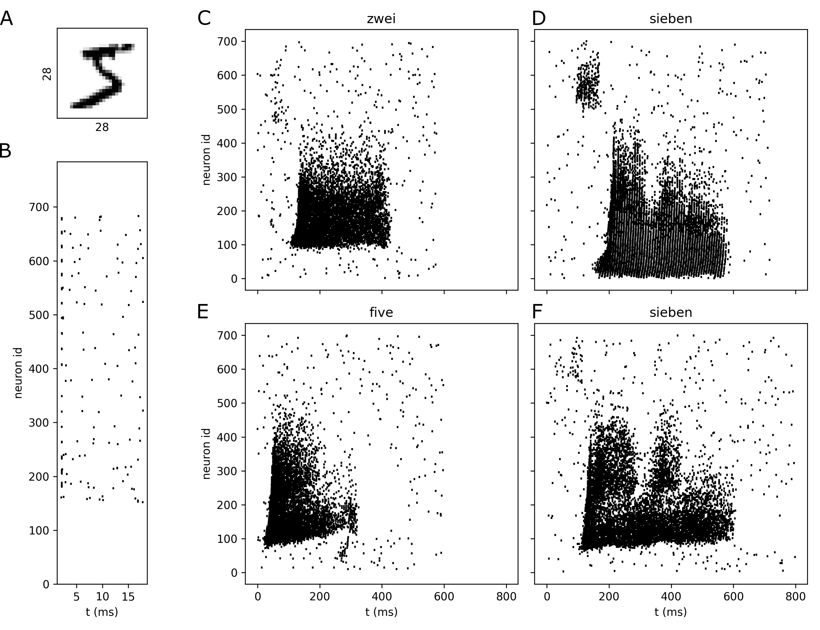
Figure 1: Examples of the MNIST and SHD data and encoding. (A) example of a $28\times 28$ MNIST gray scale image. (B) Spike encoding of the image in A), using the formula $t_{i}=\frac{255-x_{i}}{255}(T_{\text{trial}}-4$ ms$)+2$ ms, where $x_{i}$ is the grey level of the $i$th pixel in a row-wise translation through the MNIST image. (C-F) example SHD inputs for the spoken digits marked on top. Note the similarities and dissimilarities of the same spoken digit "sieben" in examples D) and F).

2 Results

Having implemented EventProp in GeNN we can explore larger and more difficult learning benchmarks. We first reproduced the results of [34] on the latency encoded MNIST dataset. The latency encoded MNIST data set consists of spiking input patterns where each of $28\times 28=784$ input neurons represents one of the pixels of the MNIST [20] pictures of handwritten digits. Each neuron fires at most once, the dark pixels earlier and lighter pixels later, see Figure 1A,B for details. We used the average cross-entropy loss

$${\cal L}_{\text{x-entropy}}=-\frac{1}{N_{\text{batch}}}\sum_{m=1}^{N_{\text{batch}}}\int_{0}^{T}\log\left(\frac{\exp\left(V_{l(m)}^{m}(t)\right)}{\sum_{k=1}^{N_{\text{class}}}\exp\left(V_{k}^{m}(t)\right)}\right)\,dt$$ (1)

that integrates a cross-entropy term of the output neurons’ membrane potentials over the duration of the trial. Here, $N_{\text{batch}}$ is the number of trials in a mini-batch, $m$ is the index of each trial, $T$ is the trial duration, $V^{m}_{*}$ is the output voltage of output neuron $*$ in the $m$th trial, and $l(m)$ denotes the correct label in trial $m$. This loss function is of the standard form supported by EventProp (Wunderlich and Pehle [34], equation (1)),

$${\cal L}=l_{p}(t^{\text{post}})+\int_{0}^{T}l_{V}(V(t),t)dt$$ (2)

with $l_{p}=0$ and

$$l_{V}=-\frac{1}{N_{\text{batch}}}\sum_{m=1}^{N_{\text{batch}}}\log\left(\frac{\exp\left(V_{l(m)}^{m}(t)\right)}{\sum_{k=1}^{N_{\text{class}}}\exp\left(V_{k}^{m}(t)\right)}\right).$$ (3)

Hence, the EventProp updates $\frac{\partial l_{V}}{\partial V}$ can be derived and applied to the dynamics of $\lambda_{V}$ of the output neurons (see table 1, equation (iii)). We implemented these updates in our PyGeNN EventProp implementation [26] and applied the learning rule in a three layer feedforward LIF network (784 – 128 – 10 neurons) to the latency encoded MNIST task. We found that we could achieve a similar classification performance on the test set ($97.8\pm 0.1$% correct – mean $\pm$ standard deviation in 10 repeated runs) as Wunderlich and Pehle [34] achieved with a not further specified implementation of a loss function based on the maximum of output voltages ($97.6\pm 0.1$% correct). This independently reproduces their work and demonstrates that our discrete time GPU implementation with $1$ ms timesteps is sufficiently precise to reach the same performance as their more exact event-based simulations.

We then considered the Spiking Heidelberg Digits (SHD) data set [5] which was generated from high quality speech recordings of 12 subjects pronouncing the digits $0$ to $9$ in both German and English. The recordings were processed through a cochlea model to yield spike patterns of $700$ input neurons of durations of a few hundred to almost $1400$ ms, depending on digit, language and speaker, see Figure 1C-F. The dataset has 8156 training examples and 2264 test samples. Two of the twelve speakers only feature in the test set, making the SHD benchmark less prone to overfitting if used appropriately. The goal in this benchmark is to classify the 20 spoken digits based on these spatio-temporal spike patterns.

We again used gradient descent with EventProp and the ${\cal L}_{\text{x-entropy}}$ loss and attempted to train a variety of three-layer networks with differently sized hidden layers both with and without recurrent connectivity, and a variety of meta-parameter values. However, we observed that the neural networks did not learn and performed close to chance level (e.g. training performance $10.9\pm 1.3$% correct after 200 epochs – mean $\pm$ standard deviation in 10 repeated trials – for a feedforward network with 256 hidden neurons). Chance level is $5$%. The example result was generated with train_test_SHD_from_json.py test_avg_xentropy/test_axe0.json test_axe0). In order to understand this failure, we inspected the learning dynamics of the network in more detail.

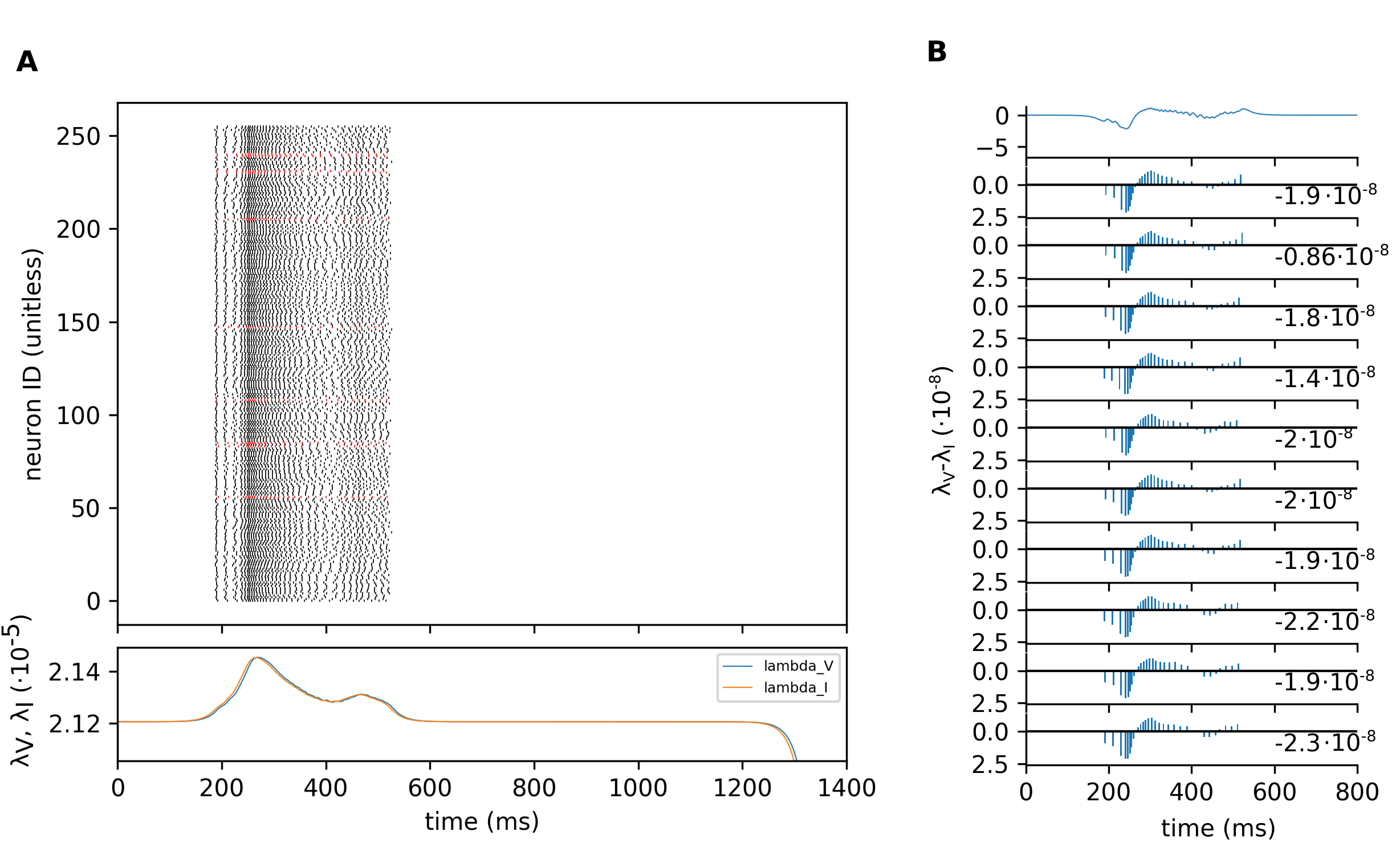
Figure 2: Illustration of the mechanism that leads to unhelpful spike deletions in hidden neurons. (A) Spike rater of hidden neurons for one input (top) and $\lambda_{V}$, $\lambda_{I}$ in the corresponding backwards pass. During backwards integration, $\lambda_{V}$ increases rapidly from 0 to the value corresponding to all output voltages being $0$. $\lambda_{I}$ follows $\lambda_{V}$. When the stored spikes are encountered, $\lambda_{V}$, $\lambda_{I}$ increase further as the model is not yet trained and the correct output voltage does not dominate in the response. (B) the difference $\lambda_{V}-\lambda_{I}$ that is transported to the neurons in the hidden layer. Top panel, entire time series, other panels the individual values when transported during a stored spike, shown as bars. We show this for the $10$ hidden neurons that were the most active on average for the input class of this example (class 7, spoken "seven") during the first two mini-batches (64 input presentations total). These neurons are highlighted in red in A). The figure was generated with test_avg_xentropy/plot_lambda_analytics.py and using the outputs test_axe1_lbdfig_trb_56.png and test_axe1_lV-lI_fig_trb_56.png.

We examined the gradient flow from the output to the hidden layer. During EventProp’s backward pass, gradients are communicated from an output neuron $j$ towards a hidden neuron $i$ by adding $w_{ji}(\lambda_{V,j}-\lambda_{I,j})$ to $\lambda_{V,i}$ at each point in backward time where a stored pre-synaptic spike was recorded during the previous forward pass. In turn, $\lambda_{V,i}$ drives $\lambda_{I,i}$, which drives the loss gradient term with respect to weights of synapses into hidden neuron $i$, see equation (v) in table 1. Accordingly, input synapses to hidden neuron $i$ with positive weight will be strengthened if $\lambda_{V,i}>0$ drives $\lambda_{I,i}>0$, and input synapses with negative weights will be weakened. This means $\lambda_{V,i}>0$ drives the hidden neuron to receive more positive input and spike earlier. The converse is true if $\lambda_{V,i}<0$ which leads to less positive input and later spiking. By inspecting $\lambda_{V,j}-\lambda_{I,j}$ at the spike times of the hidden neurons, we can hence observe the trend of whether input to hidden neurons will become more positive or more negative through learning.

Figure 2 shows an example of a trial in the early learning phase. Figure 2A shows a spike raster of hidden neuron activity (top) in response to an input digit in trial $n$ and the matching backward pass of the correct output neuron $l(n)$ (bottom) that is calculated during the next trial. Note, that the backward pass is plotted against forward time, i.e. integration proceeds from the right to the left. In this example, the correct neuron’s membrane potential does not dominate the response and $\lambda_{V,l(n)}$, and hence $\lambda_{I,l(n)}$ increase during the period where input and hidden spikes occur. Figure 2B Shows the difference $\lambda_{V,l(n)}-\lambda_{I,l(n)}$ (top panel) and the values that hence contribute to the signal transported to hidden neurons for the 10 hidden neurons that initially are the most active for class $l(n)$ ($10$ remaining panels, corresponding to neurons marked by red spikes in 2A). The overall sum of the transmitted $\lambda_{V,l(n)}-\lambda_{I,l(n)}$ values is shown to the right and is negative for all $10$ neurons, mostly because the early spike bout in the trial is more dense than the tail of spikes at the end of the trial and in this example the response was not yet appropriate: $\lambda_{V}$ increased above the ‘steady state’ value of all output voltages $=0$. This implies that the hidden neurons with a positive weight to the correct output neuron will be subdued and the activity of neurons with negative weights to the correct output neuron will be increased after learning. In other words, the most active neurons that presumably represent the relevant input best are switched off if they already connect with the correct sign to the correct output neuron and others that suppress the correct output neuron will be switched on – contrary to what one would expect.

For other trials there can be mixed positive and negative sums of transported $\lambda_{V,l(n)}-\lambda_{I,l(n)}$ or they can all be positive. In the overall balance, however, we numerically observe that hidden neurons receive less excitation over time and many of them fall silent. This in itself can cause failure but normally can be corrected with regularisation in the hidden layer (see Methods). However, in this case, while regularisation does avoid silencing of the hidden layer, it does not enable successful learning of the task. It turns out that due to the process described above, the downward pressure on hidden neurons is particularly strong for those neurons that have positive weights onto the correct output neuron, while the regularisation ensures activity recovery equally for all neurons.

To investigate this effect more explicitly we trained the network with a single input class (class 0, spoken “Null”) and inspected the relationship between the activity of hidden neurons and the weights from hidden neurons to the correct output neuron $0$. As seen in Figure 3 there is a clear negative correlation between the observed number of spikes in the hidden neurons (Figure 3B,C) and their output weights onto output neuron $0$ (Figure 3A, Pearson correlation coefficient $-0.707$). In other words, the highest output weights are from hidden neurons that do no longer respond to the class of inputs that the output neuron is supposed to represent – they have been switched off due to the gradient descent in the hidden layer.

The underlying reason why (stochastically) following the exact gradient of ${\cal L}_{\text{x-entropy}}$ leads to this failure to reduce the loss and learn the task is quite fundamental. By its nature, the exact gradient does not include information about the creation or deletion of spikes, only information about the change of the loss due to changes of spike timing of existing spikes with changes in weights. Furthermore, the gradient with respect to the spike timings of the hidden layer leads along a direction in the loss landscape where desirable spikes (of hidden neurons that drive the correct output neuron strongly) tend to be destroyed. The driving force behind these detrimental directions in weight space is the structure of the loss function. To gain a bit more intuition about this, note that the cross-entropy term in the integral has diminishing returns in terms of loss reduction when additional spikes occur at the same time. On the flipside, the silent periods before and after the spike pattern within a trial are areas where the loss term is large and cannot be reduced. In combination, the gradient on this loss function is such that when the cross-entropy term drops during the trial due to a correct response, weights will be changed such that hidden spikes are spread out (to avoid the diminishing returns) and pushed into the empty spaces to reduce loss there. This can lead to positive or negative total weight change. When the cross-entropy term increases above its baseline level, i.e. in trials where the correct output neuron’s voltage does not yet dominate during hidden layer spiking, hidden spikes are pushed together and away from the silent periods (using the diminishing returns to diminish the large loss due to their causing the wrong response). Due to the stronger spiking at the start of the response, this mostly leads to an overall negative change of the drive to the hidden neurons. In the balance, this leads to a total downward pressure onto the wrong neurons and the failure of learning. Note, that this description is somewhat simplified as we have not discussed all cases and influences of other output neurons but the numerical evidence of anti-correlations between firing rates and weight values is striking.

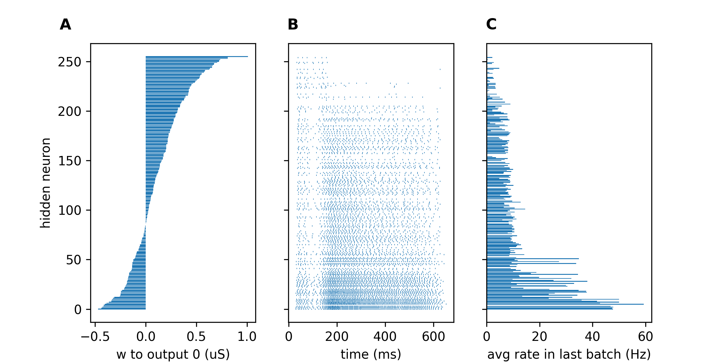
Figure 3: Illustration of the unhelpful opposing forces on hidden to output weights and hidden neuron activities. (A) hidden to output weights after $30$ epochs of training with class $0$ inputs, ordered by the weights values. (B) An example spike pattern of hidden neurons in response to an input of class $0$ in the last mini-batch. Neurons are ordered as in A). (C) averaged firing rate of hidden neurons during the last mini-batch, again ordered as in A). Results were produce by test_avg_xentropy/plot_weight_activity_correlation.py using data from a run with train_SHD_from_json.py test_axe2.json test_axe2.

Another indirect confirmation of this explanation comes from an experiment where the network is trained on the first $400$ ms of each SHD digit. In this case, the detrimental effects caused by the potentially extended silent period at the end of the trial are removed. Correspondingly, we see a somewhat better performance of the network (training $30.2\pm 1.2$% correct – mean $\pm$ standard deviation in 10 repeated trials, produced from train_test_SHD_from_json.py test_axe3.json test_axe3).

In order to avoid the problems incurred with ${\cal L}_{\text{x-entropy}}$ we need to remove the arguably unnecessary goal of classifying well across the entire duration of the trial, in particular where this is impossible during periods where input and hidden layers are silent.

A natural loss function to consider with this goal in mind is the cross-entropy of the sum or integral of the membrane potentials of the output neurons, also known to work with BPTT [40],

$${\mathcal{L}_{\text{sum}}}=-\frac{1}{N_{\text{batch}}}\sum_{m=1}^{N_{\text{batch}}}\log\left(\frac{\exp\left(\int_{0}^{T}V_{l(m)}^{m}(t)dt\right)}{\sum_{k=1}^{N_{\text{out}}}\exp\left(\int_{0}^{T}V_{k}^{m}(t)dt\right)}\right),$$ (4)

where $V_{k}^{m}$ is the membrane potential of the $k$th non-spiking output neuron in trial $m$ and $T$ denotes the duration of each trial.

With ${\cal L}_{\text{sum}}$, the contribution of each spike does now (almost) not depend on when it occurs, so that there is (almost) no pressure for changes of spike timings of hidden neurons. However, this loss function is not supported in the normal EventProp algorithm as it is not of the shape (2). In order to be able to use loss functions of this type we will derive a generalised EventProp scheme in the next section.

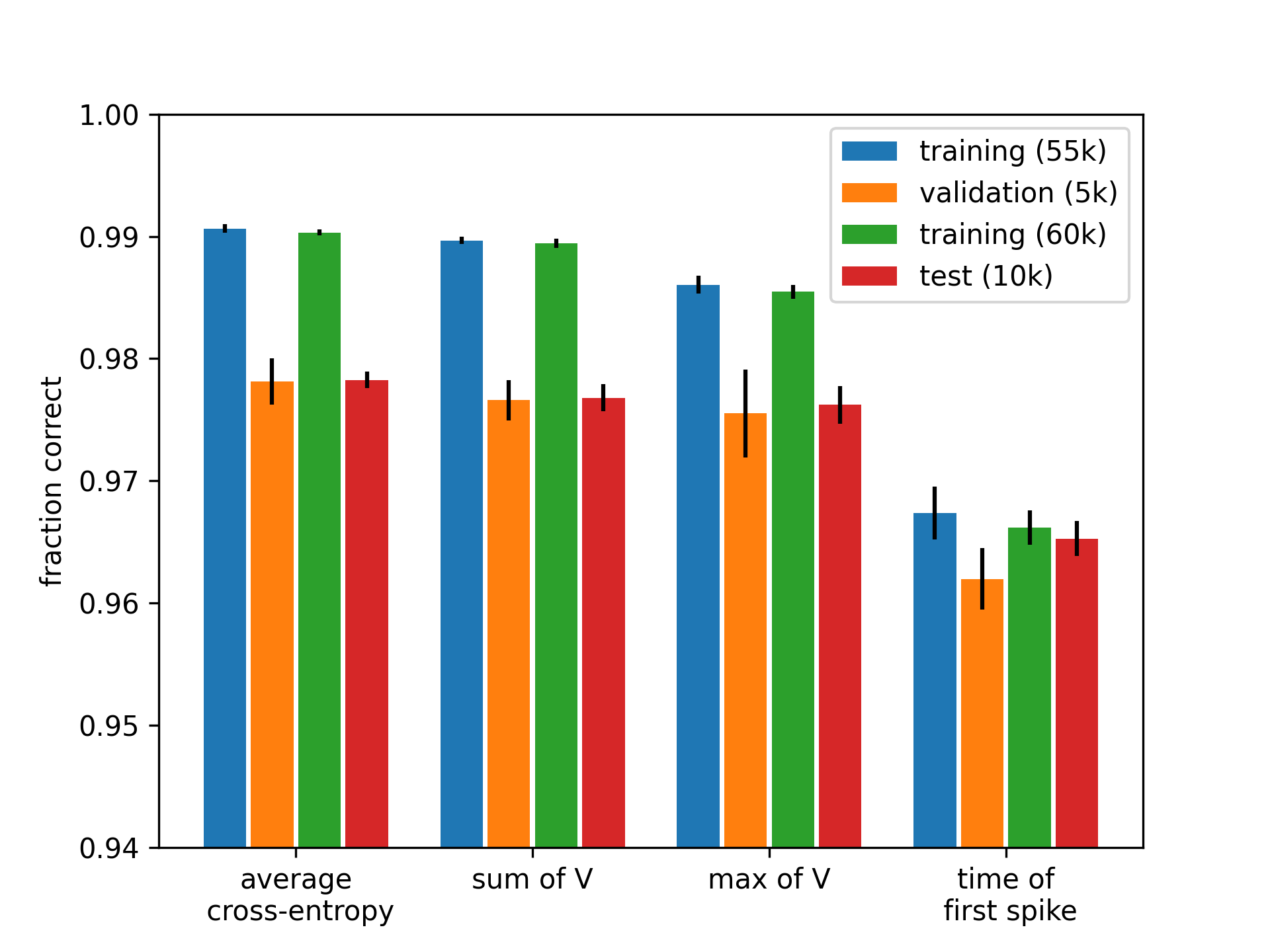
Figure 4: Overview of the classification performance of a feedforward EventProp network on the latency encoded MNIST dataset. Bars are the mean of $10$ runs and errorbars the standard deviation. All training was for $50$ epochs. There was no regularisation in the hidden layer except for when ${\cal L}_{\text{time}}$ was used. In this case $k_{\text{reg}}=10^{-8}$ and $\nu_{\text{hidden}}=4$. Results were produced with train_test_MNIST_x.py, where x is avg_xentropy, sum, max, first_spike respectively.

2.1 Additional loss functions in EventProp

The EventProp learning algorithm was formulated for loss functions of the form (2). Here, we extend the algorithm so it can also be applied to losses of the shape

$${\cal L}_{F}=F\left(\textstyle\int_{0}^{T}l_{V}(V(t),t)\,dt\right),$$ (5)

where $F$ is a differentiable function and $l_{V}$ can be vector-valued, e.g. $l_{V}=V$ as in the loss functions used in our investigations below. In brief, we can use the chain rule to calculate

$$\frac{d{\cal L}_{F}}{dw_{ji}}=\frac{\partial F}{\partial\left(\int_{0}^{T}l_{V}\,dt\right)}\cdot\frac{d\left(\int_{0}^{T}l_{V}\,dt\right)}{dw_{ji}}.$$ (6)

The expression $\int_{0}^{T}l_{V}dt$ is of the shape of supported loss functions in the original EventProp algorithm and we can calculate $\frac{d\left(\int_{0}^{T}l_{V}\,dt\right)}{dw_{ji}}$ using it. This leads to as many separate models as $l_{V}$ has dimensions but because equation (6) is linear in $\frac{d\left(\int_{0}^{T}l_{V}\,dt\right)}{dw_{ji}}$, and equations (iii) and (iv) in table 1 are linear in $\lambda_{V}$ and $\lambda_{I}$, we can “push this extra complexity into the dynamics” by recombining the adjoint variables $\lambda$ in the individual model copies into ‘aggregate’ adjoint variables to recover a single EventProp backward pass of the form

$$\tau_{\text{mem}}\tilde{\lambda}_{V,j}^{\prime} =-\tilde{\lambda}_{V,j}-\sum_{n}\frac{\partial F}{\partial(\int l_{V}^{n}dt)}\frac{\partial l_{V}^{n}}{\partial V_{j}},$$ (7)

$$\tau_{\text{syn}}\tilde{\lambda}_{I,j}^{\prime} =-\tilde{\lambda}_{I,j}+\tilde{\lambda}_{V,j},$$ (8)

$$\frac{d{\cal L}}{dw_{ji}} =-\tau_{\text{syn}}\sum_{t\in t_{\text{spike}}(i)}\tilde{\lambda}_{I,j}(t),$$ (9)

where (7) replaces equation (iii), (8) equation (iv), and (9) equation (v) in table 1. See Appendix A for a detailed derivation of these equations.

Equipped with the extended scheme we were able to implement EventProp for three additional loss functions. We can now make decisions based on the integrated voltage of the non-spiking output neurons and use the sum loss (4). We can also make classifications based on the maximum membrane potential of the non-spiking output neurons and use the loss

$${\cal L}_{\text{max}}=-\frac{1}{N_{\text{batch}}}\sum_{m=1}^{N_{\text{batch}}}\log\left(\frac{\exp\left(\max_{[0,T]}V_{l(m)}^{m}(t)\right)}{\sum_{k=1}^{N_{\text{class}}}\exp\left(\max_{[0,T]}V_{k}^{m}(t)\right)}\right),$$ (10)

where again $V_{k}^{m}$ is the membrane potential of the $k$th non-spiking output neuron in trial $m$ and $T$ denotes the duration of each trial. Finally, if we use spiking output neurons and make the classification decision depending on which of the output neurons fires the first spike, we can use the time to first spike loss

$${\cal L}_{\text{time}}=-\frac{1}{N_{\text{batch}}}\sum_{m=1}^{N_{\text{batch}}}\left[\log\left(\frac{\exp(-t^{m}_{l(m)}/\tau_{0})}{\sum_{k=1}^{N_{\text{class}}}\exp(-t_{k}^{m}/\tau_{0})}\right)-\alpha\left(\exp(t^{m}_{l(m)}/\tau_{1})-1\right)\right]$$ (11)

where $t_{k}^{m}$ is the first spike in output neuron $k$ and trial $m$ and $l(m)$ is the correct label for trial $m$. The first loss term is a cross-entropy loss pushing spikes of the correct output neuron to earlier times relative to spikes of other output neurons. The second term ensures that the spikes of the correct output neuron are pushed to earlier times to avoid all output spikes floating beyond the end of the trial. $\alpha$, $\tau_{0}$ and $\tau_{1}$ are hyper-parameters of the loss function, $N_{\text{class}}$ is the number of classes and $N_{\text{batch}}$ the number of trials in a mini-batch.

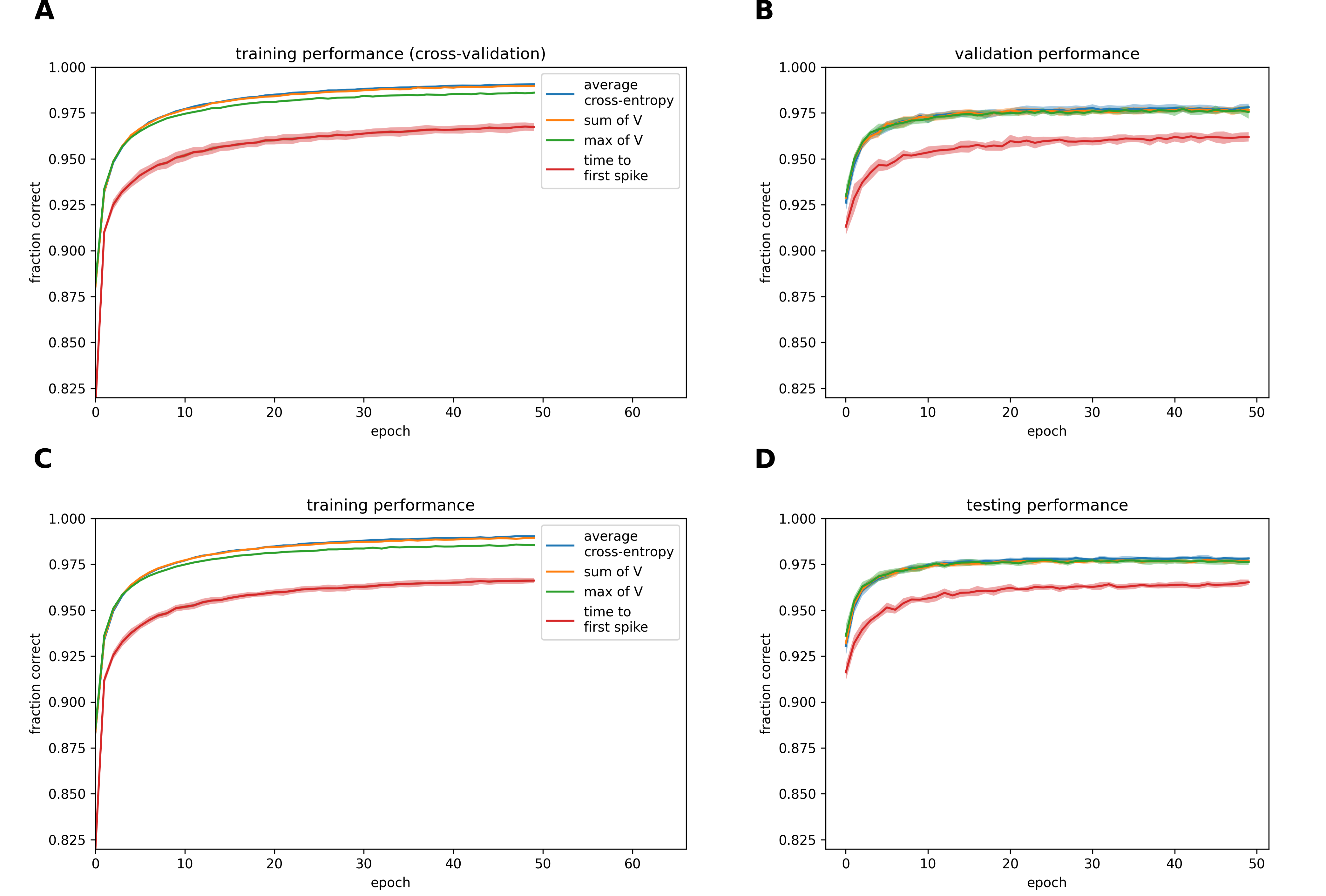
Figure S1: Learning curves for the latency MNIST task. (A) training performance during cross-validation runs with 55,000 to 5,000 random split on the training set. Curves are the mean of 10 folds, areas the standard deviation across folds. (B) matching validation performance. (C) Training performance for the entire training set. (D) testing performance at the end of each epoch.

We implemented this larger set of loss functions and again addressed the latency MNIST task. We found that all considered loss functions performed reasonably well on this task, with a slightly lower performance with the ${\cal L}_{\text{time}}$ loss (Figure 4). The displayed performance could be achieved with minimal hand-tuning of meta-parameters and learning occurred fast and reliably (see learning curves in Supplementary Figure S1).

We then returned to the SHD benchmark. We adjusted meta-parameters of the models with each of the loss functions using grid searches in a 10-fold cross-validation approach: In each fold we trained the network on $9$ of the speakers and tested it on the inputs derived from the $10$th speaker (2 speakers are exclusive to the test set that we only used later). After adjusting meta-parameters this way (see tables 1, 2), we then also measured training and testing performance with the full training and test set. The result are shown in Figure 5. The results for the failing ${\cal L}_{\text{x-entropy}}$ loss were omitted in this figure to avoid too much clutter.

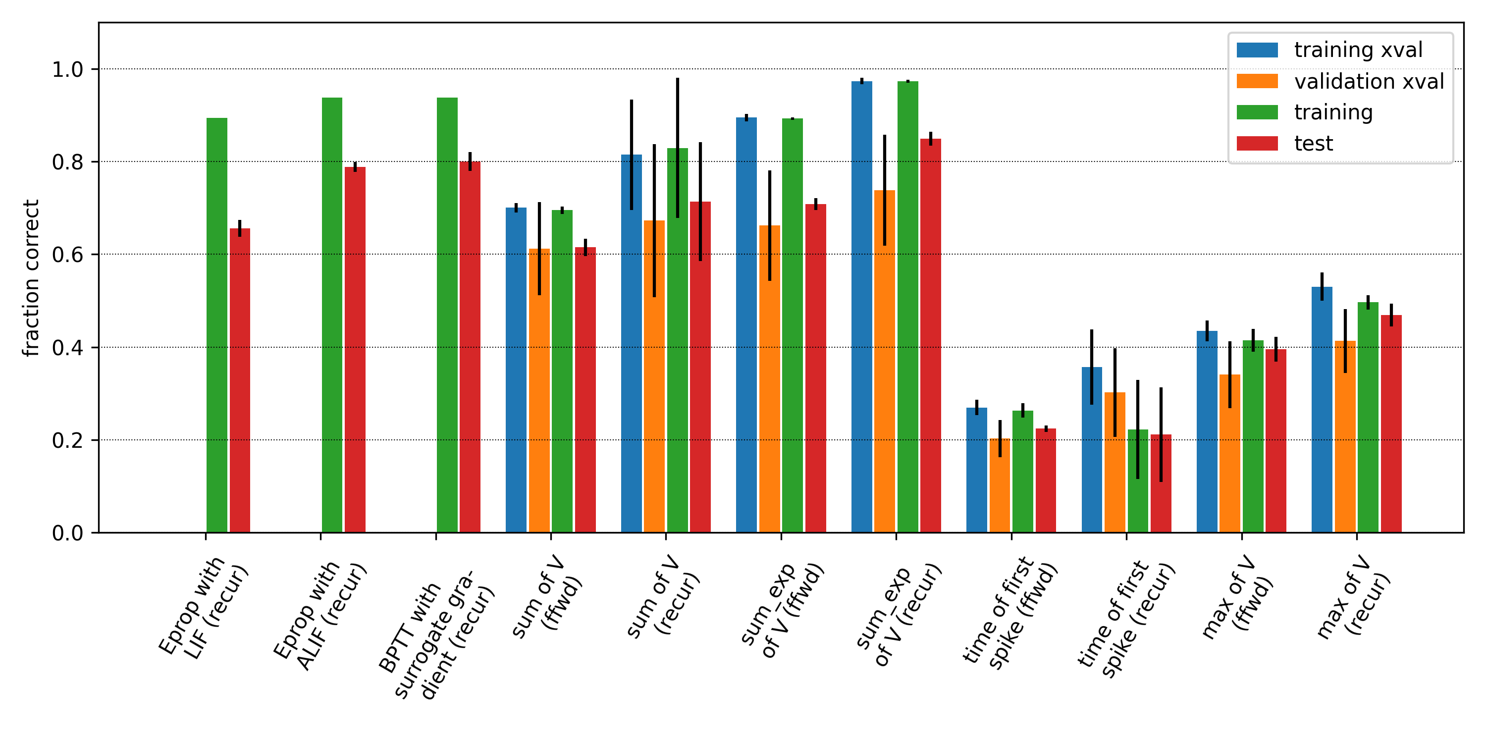
Figure 5: Summary of SHD classification results. The back-propagation through time with surrogate gradient result is from [40]. "ffwd" are feed-forward networks, "recur" recurrent networks. "xval" refers to "leave one speaker out" cross-validation (see methods). The bars are the average fraction of correctly predicted digits after $300$ training epochs, for the cross-validation averaged over the $10$ folds of left out speakers, for the full training and testing averaged over $10$ runs with different random seeds. We used up to $512$ samples from the left out speaker for validation. The error bars are standard deviations for the same repeats. In the cross-validation, mean and standard deviation are additionally averaged across two runs with different seeds. The parameters for the different models leading to these results are summarised in tables 2,3. Results were analysed with get_best_values_paras.py and subsequently plotted with plot_SHD_summary_v3.py.

The classification success of the different loss functions varies. Apart from the completely failing ${\cal L}_{\text{x-entropy}}$ loss, the worst performance and least reliability in performance was observed for the ${\cal L}_{\text{time}}$ loss, followed by the ${\cal L}_{\text{max}}$ loss. The ${\cal L}_{\text{sum}}$ loss performed competitively with respect to the results reported in the literature [40] and the e-prop results obtained in our lab [19], in particular with recurrent connectivity. However, the performance was not quite as good as the competitors. When we inspected the learning dynamics (Figure 6), we observed that learning for ${\cal L}_{\text{sum}}$ is comparatively slow in spite of the fact that we ran the model with an increased learning rate $\lambda=5\cdot 10^{-3}$ (see table 2). The optimised regularisation strength of the hidden layer is also orders of magnitudes smaller in this model than in the others. Both observations may be indicative of very weak gradients flowing from the output layer towards the hidden layer. On reflection, this effect can be easily understood when realising that due to the shape of ${\cal L}_{\text{sum}}$ the timing of hidden spikes does (almost) not matter for their effect on the overall loss. Every post-synaptic potential (PSP) causes the same added (or subtracted for negative synaptic weight) area under the membrane potential and hence the same increase or reduction in loss. The only exception to this is that the PSPs are cut off at trial end so that earlier spikes contribute a tiny bit more as less area is cut off. This cut-off causes a minute contribution to the gradient to move hidden spikes earlier or later.

Based on this insight, we then tried to improve the gradient flow to the hidden layer by adding a weighting function to ${\cal L}_{\text{sum}}$ that would make earlier PSPs more effective for increasing or reducing the loss. We tried four different weightings, linearly decreasing, exponentially decreasing, sigmoid and proportional to the number of input spikes at each timestep. In numerical experiments, the exponential weighting appeared to perform best leading to our use of the loss

$${\mathcal{L}_{\text{sum\_exp}}}=-\frac{1}{N_{\text{batch}}}\sum_{m=1}^{N_{\text{batch}}}\log\left(\frac{\exp\left(\int_{0}^{T}e^{-t/T}V_{l(m)}^{m}(t)dt\right)}{\sum_{k=1}^{N_{\text{out}}}\exp\left(\int_{0}^{T}e^{-t/T}V_{k}^{m}(t)dt\right)}\right).$$ (12)

As shown in Figure 5 this loss function leads to a learning network that can beat the previous SNN result with BPTT [40] and our own results with e-prop [19]. Additionally, learning is much faster and more reliable (see Figure 6).

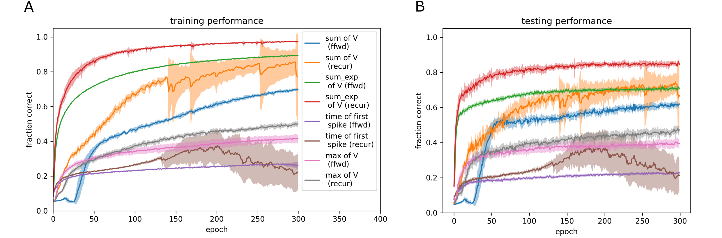
Figure 6: Fraction of correct digit recognition during the training process. (A) fraction of correctly predicted digits in the training set. (B) fraction of correctly predicted digits in the testing set. The lines are the mean of 10 repetitions with different random seeds. The shaded regions are the standard deviation around the mean for the 10 repetitions. The parameters used for each model are the same as for figure 5. Results were analysed with get_best_values_paras.py and subsequently plotted with plot_SHD_curves_v3.py

Table 2: Major model parameters

Name	Description	Value MNIST	Value SHD
$\tau_{\text{mem}}$	timescale of membrane potential	$20$ ms	$20$ ms
$\tau_{\text{syn}}$	synaptic timescale	$5$ ms	$5$ ms
$\vartheta$	firing threshold	$1$ mV	$1$ mV
$V_{\text{reset}}$	reset for membrane potential	$0$ mV	$0$ mV
$T$	trial duration	$20$ ms	$1400$ ms
$\mu_{i\_h}$	Mean initial weight value input to hidden	$0.045$ mV	$0.03$ mV
$\sigma_{i\_h}$	Standard deviation of initial weight value input to hidden	$0.045$ mV	$0.01$ mV
$N_{\text{hidden}}$	Number of hidden neurons	$128$	$256$
$\mu_{h\_o}$	Mean initial weight value hidden to output	$\!\!\!\!\left\{\begin{array}[]{ll}\!\!\!0.9\text{ mV}&\!\!\text{if }{\cal L}_{\text{time}}\\ \!\!\!0.2\text{ mV}&\!\!\text{o.w.}\end{array}\right.$	table 2
$\sigma_{h\_o}$	Standard deviation of initial value hidden to output	$\!\!\!\!\left\{\begin{array}[]{ll}\!\!\!0.03\text{ mV}&\!\!\text{if }{\cal L}_{\text{time}}\\ \!\!\!0.37\text{ mV}&\!\!\text{o.w.}\end{array}\right.$	table 2
$\mu_{h\_h}$	standard deviation of initial weight value hidden to hidden	–	$0$ mV
$\sigma_{h\_h}$	standard deviation of initial weight value hidden to hidden	–	$0.02$ mV
$p_{\text{drop}}$	Dropout probability for input spikes	$0.2$	$0$
$\nu_{\text{hidden}}$	target hidden spike number for regularisation	$4$ if ${\cal L}_{\text{time}}$	$14$
$\eta$	Learning rate	$\!\!\!\!\left\{\begin{array}[]{ll}\!\!\!5\cdot 10^{-3}&\!\!\text{if }{\cal L}_{\text{time}}\\ \!\!\!10^{-2}&\!\!\text{o.w.}\end{array}\right.$	table 2
$\tau_{0}$	Parameter of timing loss ${\cal L}_{\text{time}}$	$1$ ms	$1$ ms
$\tau_{1}$	Parameter of timing loss ${\cal L}_{\text{time}}$	$3$ ms	$100$ ms
$\alpha$	Parameter of timing loss ${\cal L}_{\text{time}}$	$3.6\cdot 10^{-4}$	$5\cdot 10^{-5}$
$\beta_{1}$	Adam optimiser parameter	$0.9$	$0.9$
$\beta_{2}$	Adam optimiser parameter	$0.999$	$0.999$
$\epsilon$	Adam parameter	$10^{-8}$	$10^{-8}$
$\Delta t$	simulation timestep	$1$ ms	$1$ ms
$N_{\text{batch}}$	min-batch size	$32$	table 2
$N_{\text{epoch}}$	number of training epochs	$50$	$300$
$f_{\text{shift}}$	amplitude of "frequency shift" augmentation	–	$40$

Table 3: Specific parameters of different SHD models

Parameter	Models
loss	${\cal L}_{\text{sum}}$		${\cal L}_{\text{sum\_exp}}$		${\cal L}_{\text{time}}$		${\cal L}_{\text{max}}$
architecture	ffwd	recur	ffwd	recur	ffwd	recur	ffwd	recur
$N_{\text{batch}}$	$256$	$256$	$32$	$32$	$32$	$32$	$256$	$256$
$k_{\text{reg}}$	$10^{-12}$	$5\cdot 10^{-13}$	$5\cdot 10^{-10}$	$5\cdot 10^{-10}$	$2\cdot 10^{-07}$	$2\cdot 10^{-07}$	$2\cdot 10^{-10}$	$5\cdot 10^{-9}$
$\mu_{h\_o}$	$0$	$0$	$0$	$0$	$1.2$	$1.2$	$0$	$0$
$\sigma_{h\_o}$	$0.03$	$0.03$	$0.03$	$0.03$	$0.6$	$0.6$	$0.03$	$0.03$
$\eta$	$0.005$	$0.005$	$0.001$	$0.001$	$0.001$	$0.001$	$0.002$	$0.002$

3 Discussion and Conclusions

In this article we have presented learning results for the EventProp algorithm implemented in GeNN. We have identified issues when training a small spiking neural network with the exact gradient descent calculated with EventProp when using the average cross-entropy loss function ${\cal L}_{\text{x-entropy}}$. In essence the problem we identified was that the exact gradient would inadvertently lead to weight updates that eventually silenced the hidden neurons that were best placed to represent a given class of inputs and drive the correct output. Underlying this unhelpful learning dynamics were two fundamental factors. One is that by its nature the exact gradient of a loss function in an SNN does not contain information about spike creation or spike loss when input weights are increased or decreased. The other factor was the combination of the task structure and the choice of the ${\cal L}_{\text{x-entropy}}$ loss function. As explained in detail in the Results, the diminishing effect of synchronous excitation on the correct output neuron and the large losses incurred during the silent periods in the beginning and at the end of a trial led to gradients that moved spikes in the hidden layer forwards and backwards in an unhelpful way that eventually led to the unfortunate silencing of important hidden neurons. While the specific effect in this particular model is very subtle and depends on many details, such as the number of input spikes early and later in each trial, fundamentally, the problem is that the loss function incorporated more structure than was needed for the successful completion of the task. The classification decision is always based on the comparison of properties of the output neurons’ membrane potentials and only depend on which was the highest, not their actual values. Driving up the membrane potential, or derived terms like the cross-entropy loss, to ever higher values and especially trying to do so for e.g. the silent periods, is counter-productive and does not assist the learning.

We overcame the shortcomings by deriving an extended EventProp algorithm that allows more general loss functions and found that the cross-entropy loss of average output voltages ${\cal L}_{\text{sum}}$ allowed successful learning but learning was arguably slow and somewhat unreliable and performance slightly below competing learning rules. We identified that one issue was now an almost complete lack of gradient flow towards the hidden layer. So we went full circle and now introduced a beneficial weighting term into the loss function that pushed helpful hidden spikes forward in time and inadvertently also created more of these spikes. With the weighted loss function ${\cal L}_{\text{sum\_exp}}$ we finally observed fast, reliable and competitive learning on the SHD problem with a headline $97.3\pm 0.3$% correct training and $84.8\pm 1.5$% correct testing performance. It is worth noting once more that we have here added extra complexity to induce a beneficial deformation of the loss landscape that avoided undesired spike loss and generated beneficial additional spikes, both effects that cannot be directly induced by a loss function on an SNN if using exact gradients.

A few other observations are important. We ran the forward pass and previous’ mini-batch’s backward pass computations in parallel in the same neuron model for efficiency. This implies that the weight updates are applied one mini-batch later than in the normal sequential forward pass – backward pass scheme. In initial testing with the MNIST task, we did not find any measurable difference between the two approaches.

We have tried different types of data augmentations in the SHD task, as described in the Methods but found that within the range of parameter scans we were able to compute, only the random shift augmentation made a measurable difference. This contrasts somewhat with the results reported in [5], where an overlapping but not identical set of augmentations were used. A detailed analysis of appropriate augmentations for SHD and tasks of similar nature is an important future research direction. The remaining sizeable gap between training and validation/testing errors suggests that there is still a measurable amount of overfitting in the present setup.

We also implemented and tested different types of regularisation in the hidden layer, based on different combinations of the overall number of spikes in a trial, the number of spikes in individual neurons in each trial and similar quantities averaged across the mini-batch. We found that the simple regularisation based on the average number of spikes of individual hidden neurons across the mini-batch as described in the methods provided a reliable stabilisation of the activity in the hidden layer and was sufficient to allow learning to proceed. An urgent future research direction is, however, the investigation of more principled ways of finding the right regularisation strength in the hidden layer. The ideal strength of the regularisation loss term depends intimately on the details of the main loss function and the resulting gradient flow. It would be desirable to find ways of regularisation that did not necessitate the grid searches for the correct regularisation strength employed here.

The exponentially weighted sum loss was the most successful loss function among those we investigated and allows both, rapid and stable learning. We tried a few other weighting schemes, linear weighting across the trial and weighing loss terms in proportion to the instantaneous firing rate in the input neurons. The latter was motivated by the idea that meaningful responses would occur mostly when there is informative input and less so when the input layer is silent. We found, however, that the exponential weighting worked best in the cross-validation assessment and it was therefore selected for the final assessment on the test set.

The EventProp implementation in GeNN introduced in this paper is efficient and makes use of GeNNs advanced algorithms for event propagation when spikes occur in forward and backward passes. Nevertheless, a full $10$-fold cross-validation with $300$ epochs per fold still takes about $16$ hours on an A100 GPU highlighting that this type of research remains compute-intensive. A detailed comparison of runtimes in comparison to other learning rules such as e-prop will be published separately.

In conclusion, while the ability to calculate exact gradients efficiently using the EventProp method is attractive, the exact gradient is agnostic of spike creation and deletion and in combination with task and model details, including the exact choice of the loss function, this can lead to learning failures. In this paper we have extended EventProp to allow more general loss functions and have demonstrated on the example of the SHD classification task how ‘loss shaping’, i.e. choosing a bespoke loss function that induces beneficial gradient flows and learning dynamics, leads to competitive learning results. Whether ‘loss shaping’ can be done in a more principled way and how it carries over to deeper networks are open questions we would like to address in the near future.

4 Methods

4.1 Phantom spike regularisation

For the time to first spike loss function ${\cal L}_{\text{time}}$, there is a risk that if the correct output neuron does not spike in spite of the loss term that tries to push its spikes forward in time, there will be no valid gradient to follow. To address this issue we introduced ‘phantom spikes’ so that if the correct neuron does not spike during a trial, a regularisation loss term is added to the $\Lambda_{V}$ dynamical equation as if the neuron had spiked at time $T$.

4.2 Regularisation in the hidden layer

When hidden layer neurons spike too frequently or cease to spike, network performance degrades. We therefore introduced a regularisation term to the loss function that penalises derivations from a target firing rate,

$${\cal L}_{\text{reg}}=\frac{1}{2}k_{\text{reg}}\sum_{l=1}^{N_{\text{hidden}}}\left(\left(\frac{1}{N_{\text{batch}}}\sum_{n=1}^{N_{\text{batch}}}n^{\text{spike},n}_{l}\right)-\nu_{\text{hidden}}\right)^{2}$$ (13)

where $n^{\text{spike},n}_{l}$ denotes the number of spikes in hidden neuron $l$ in trial $n$ and $\nu_{\text{hidden}}$ represents the target number of spikes in a trial. For example, in the SHD experiments, $\nu_{\text{hidden}}=14$ corresponding to a 10 Hz target firing rate in a 1400 ms trial. $k_{\text{reg}}$ is a free parameter scaling the strength of the regularisation term. We can write

$$n^{\text{spike},n}_{l}=\int_{0}^{T}\sum_{k}\frac{V_{l}^{n}(t)}{\vartheta}\delta(t-t_{l,k}^{n})dt,$$ (14)

where $t_{k,l}^{n}$ is the $k$th spike in hidden neuron $l$ during trial $n$ and we assume that the membrane potential $V_{l}^{n}(t)$ is equal to the threshold $\vartheta$ when the spikes occur. The regularisation loss then has the shape of a function of the integral over a function of the membrane potential, so that we can use the method in Appendix A to derive jumps of

$$\lambda_{V,l}^{-}=\lambda_{V,l}^{+}-k_{\text{reg}}\left(\frac{1}{N_{\text{batch}}}\sum_{n=1}^{N_{\text{batch}}}n^{\text{spike},n}_{l}-\nu_{\text{hidden}}\right)\frac{1}{N_{\text{batch}}\vartheta}$$ (15)

at recorded spikes of the hidden neurons during the backward pass.

4.3 Augmentation

We initially investigated three types of input augmentation to lessen the detrimental effects of over-fitting.

1. The ID jitter augmentation was implemented as in [5]. For each input spike, we added a ${\cal N}(0,\sigma_{u})$ distributed random number to the index $i$ of the active neuron, rounded to an integer and created the spike in the corresponding neuron instead.

2. In the random dilation augmentation, we rescaled the spike times of each input pattern homogeneously by a factor random factor $k^{\text{scale}}$ drawn uniformly from $[k^{\text{scale}}_{\text{min}},k^{\text{scale}}_{\text{max}}]$.

3. In the random shift augmentation we globally shifted the input spikes of each digit across input neurons by a distance $k^{\text{shift}}$ uniformly drawn from $[-f_{\text{shift}},f_{\text{shift}}]$, rounded to the nearest integer.

In preliminary experiments we observed that only the random shift augmentation improved generalisation noticeably and we conducted the remainder of the research only with this augmentation.

4.4 Implementation details

We have used the GeNN simulator version 4.8.0 [37, 6] through the PyGeNN interface [17] for this research. The EventProp backward pass is implemented with additional neuron variables $\lambda_{V}$ and $\lambda_{I}$ within the neuron sim_code code snippet. For efficiency we ran the forward pass of mini-batch $i$ and the backward pass of mini-batch $i-1$ simultaneously in the same neurons. For mini-batch $0$ no backward pass is run and the backward pass of the last mini-batch in each epoch is not simulated. In initial experiments we observed no measurable difference other than reduced runtime when comparing to properly interleaved forward-only and backward-only simulations.

During training the inputs are presented in a random order in each epoch. For the weight updates we used the Adam optimizer [16]. The parameters of the simulations are detailed in tables 1 and 2. The simulation code is published on Github [26].

Simulations were run on a local workstation with NVIDIA GeForce RTX 3080 GPU, on the JADE GPU cluster equipped with NVIDIA V100 GPUs and the JUWELS-Booster system at the Jülich Supercomputer Centre, equipped with NVIDIA A100 GPUs.

Appendix

Appendix A Full derivation of extended EventProp

In this Appendix we present the detailed derivation for extending the EventProp algorithm to losses of the shape

$${\cal L}_{F}=F\left(\textstyle\int_{0}^{T}l_{V}(V(t),t)\,dt\right),$$ (16)

where $F$ is a differentiable function and $l_{V}$ can be vector-valued, e.g. $l_{V}=V$ as in the loss functions used in the main body of the paper.

Using the chain rule, we can calculate

$$\frac{d{\cal L}_{F}}{dw_{ji}}=\frac{\partial F}{\partial\left(\int_{0}^{T}l_{V}\,dt\right)}\cdot\frac{d\left(\int_{0}^{T}l_{V}\,dt\right)}{dw_{ji}}=\sum_{n}\frac{\partial F}{\partial\left(\int_{0}^{T}l_{V}^{n}\,dt\right)}\frac{d\left(\int_{0}^{T}l_{V}^{n}\,dt\right)}{dw_{ji}}$$ (17)

where $n$ labels the components of the vector-valued $l_{V}$, for instance $l_{V}$= $V_{\text{output}}$ and $n$ labels the output neurons (see below). The integrals $\int_{0}^{T}l_{V}^{n}(t)dt$ are of the shape (2) of a classic EventProp loss function, so we can use the EventProp algorithm to calculate

$$\frac{d\left(\int_{0}^{T}l_{V}^{n}\,dt\right)}{dw_{ji}}=-\tau_{\text{syn}}\sum_{t\in t_{\text{spike}}(i)}\lambda_{I,j}^{n}(t),$$ (18)

where

$$\tau_{\text{syn}}{\lambda_{I,j}^{n}}^{\prime}=-\lambda_{I,j}^{n}+\lambda_{V,j}^{n}$$ (19)

$$\tau_{\text{mem}}{\lambda_{V,j}^{n}}^{\prime}=-\lambda_{V,j}^{n}-\frac{\partial l_{V}^{n}}{\partial V_{j}}$$ (20)

With this in mind, we can then calculate the gradient of the loss function (16):

$$\frac{d{\cal L}_{F}}{dw_{ji}} =-\tau_{\text{syn}}\sum_{n}\frac{\partial F}{\partial(\int_{0}^{T}l_{V}^{n}dt)}\sum_{t\in t_{\text{spike}}(i)}\lambda_{I,j}^{n}(t)$$ (21)

$$=-\tau_{\text{syn}}\sum_{t\in t_{\text{spike}}(i)}\sum_{n}\frac{\partial F}{\partial(\int l_{V}^{n}dt)}\lambda_{I,j}^{n}(t)=-\tau_{\text{syn}}\sum_{t\in t_{\text{spike}}(i)}\tilde{\lambda}_{I,j}(t)$$ (22)

where we have defined

$$\tilde{\lambda}_{I,j}(t):=\sum_{n}\frac{\partial F}{\partial(\int l_{V}^{n}dt)}\lambda_{I,j}^{n}(t).$$ (23)

We can then derive dynamics for $\tilde{\lambda}_{I,j}$ by simply using this definition and noting that $\frac{\partial F}{\partial(\int l_{V}^{n}dt)}$ does not depend on $t$,

$$\tau_{\text{syn}}\tilde{\lambda}_{I,j}^{\prime} =\sum_{n}\frac{\partial F}{\partial(\int l_{V}^{n}dt)}\tau_{\text{syn}}{\lambda_{I,j}^{n}}^{\prime}=\sum_{n}\frac{\partial F}{\partial(\int l_{V}^{n}dt)}\left(-\lambda_{I,j}^{n}+\lambda_{V,j}^{n}\right)=-\tilde{\lambda}_{I,j}+\tilde{\lambda}_{V,j},$$ (24)

where we defined

$$\tilde{\lambda}_{V,j}:=\sum_{n}\frac{\partial F}{\partial(\int l_{V}^{n}dt)}\lambda_{V,j}^{n}.$$ (25)

That implies the dynamics

$$\tau_{\text{mem}}\tilde{\lambda}_{V,j}^{\prime} =\sum_{n}\frac{\partial F}{\partial(\int l_{V}^{n}dt)}\tau_{\text{mem}}{\lambda_{V,j}^{n}}^{\prime}=-\tilde{\lambda}_{V,j}-\sum_{n}\frac{\partial F}{\partial(\int l_{V}^{n}dt)}\frac{\partial l_{V}^{n}}{\partial V_{j}}.$$ (26)

In this fashion we have recovered an EventProp algorithm to calculate the gradient of the general loss function (16) by using equations (22),(24), and (26). Remarkably, this algorithm is exactly as the original EventProp algorithm except for the slightly more complex driving term for $\tilde{\lambda}^{\prime}_{V,j}$ in equation (26).

Appendix B Extended EventProp for specific loss functions

For the concrete example of the loss function (4), we have $l_{V}=(V_{n}^{m})$, i.e. the vector of output voltages of output neuron $n$ in each batch $m$. With respect to the mini-batch summation we typically calculate the gradient as the sum of the individual gradients for each trial in the mini-batch,

$$\frac{d{\cal L}}{dw_{ji}}=\frac{1}{N_{\text{batch}}}\sum_{m=1}^{N_{\text{batch}}}\frac{d}{dw_{ji}}\left(-\log\frac{\exp\left(\int_{0}^{T}V_{l(m)}^{m}(t)dt\right)}{\sum_{k=1}^{N_{\text{out}}}\exp\left(\int_{0}^{T}V_{k}^{m}(t)dt\right)}\right)=\frac{1}{N_{\text{batch}}}\sum_{m=1}^{N_{\text{batch}}}\frac{dF^{m}}{dw_{ji}},$$ (27)

with

$$F^{m}({\textstyle\int_{0}^{T}Vdt})=-\log\frac{\exp\left(\int_{0}^{T}V_{l(m)}^{m}(t)dt\right)}{\sum_{k=1}^{N_{\text{out}}}\exp\left(\int_{0}^{T}V_{k}^{m}(t)dt\right)}$$ (28)

and for each trial $m$ and output neuron $n$ we get

$$\frac{\partial F^{m}}{\partial(\int_{0}^{T}V_{n}^{m}dt)}=-\delta_{n,l(m)}+\frac{\exp(\int V_{n}^{m}dt)}{\sum_{k=1}^{N_{\text{class}}}\exp(\int_{0}^{T}V_{k}^{m}dt)}$$ (29)

and $\frac{\partial l_{V}}{\partial V_{j}^{m}}=\frac{\partial V_{n}^{m}}{\partial V_{j}^{m}}=\delta_{jn}$. We, therefore, can formulate the EventProp scheme

$$\frac{dF^{m}}{dw_{ji}} =-\tau_{\text{syn}}\sum_{\{t_{\text{spike}}(i)\}}\tilde{\lambda}_{I,j}^{m}(t_{\text{spike}})$$ (30)

$$\tau_{\text{syn}}\tilde{\lambda}_{I,j}^{m}{}^{\prime} =-\tilde{\lambda}_{I,j}^{m}+\tilde{\lambda}_{V,j}^{m}$$ (31)

$$\tau_{\text{mem}}\tilde{\lambda}_{V,j}^{m}{}^{\prime} =-\tilde{\lambda}_{V,j}^{m}+\delta_{j,l(m)}-\frac{\exp(\int V_{j}^{m}dt)}{\sum_{k=1}^{N_{\text{class}}}\exp(\int_{0}^{T}V_{k}^{m}dt)}.$$ (32)

i.e. there is a positive contribution $1$ for each correct output neuron and the negative fraction of exponentials for all output neurons. All other neurons do not enter the loss function directly and the loss propagates as normal from the output neurons through the $W^{T}(\lambda_{V}^{+}-\lambda_{I})$ terms. The final loss is then added up according to (27).

Another typical loss function for classification works with the maxima of the voltages of the non-spiking output neurons

$${\mathcal{L}_{\text{max}}}=-\frac{1}{N_{\text{batch}}}\sum_{m=1}^{N_{\text{batch}}}\log\frac{\exp\left(\max_{[0,T]}V_{l(m)}^{m}(t)\right)}{\sum_{k=1}^{N_{\text{out}}}\exp\left(\max_{[0,T]}V_{k}^{m}(t)\right)}$$ (33)

As already argued in [34], we can rewrite

$$\max_{[0,T]}V_{n}^{m}(t)=\int_{0}^{T}V_{n}^{m}(t)\delta(t-t_{\text{max},n}^{m})\,dt,$$ (34)

where $\delta$ is the Dirac distribution and $t_{\text{max}}$ the time when the maximum $V$ was observed. Then we can use arguments as above to find the EventProp scheme

$$\frac{d{F^{m}}}{dw_{ji}} =-\tau_{\text{syn}}\sum_{\{t_{\text{spike}}(i)\}}\tilde{\lambda}_{I,j}^{m}(t_{\text{spike}})$$ (35)

$$\tau_{\text{syn}}\tilde{\lambda}_{I,j}^{m}{}^{\prime} =-\tilde{\lambda}_{I,j}^{m}+\tilde{\lambda}_{V,j}^{m}$$ (36)

$$\tau_{\text{mem}}\tilde{\lambda}_{V,j}^{m}{}^{\prime} =-\tilde{\lambda}_{V,j}^{m}+\left(\delta_{j,l(m)}-\frac{\exp\left(\max_{[0,T]}V_{j}^{m}\right)}{\sum_{k=1}^{N_{\text{class}}}\exp\left(\max_{[0,T]}V_{k}^{m}\right)}\right)\delta\left(t-t_{\text{max},j}^{m}\right),$$ (37)

i.e. we have jumps at the times where the maximum voltages in each of the neurons occurred, with a magnitude determined by the combination of the maximum voltages of all output neurons.

Supplementary material

References

- [1] Guillaume Bellec, Franz Scherr, Anand Subramoney, Elias Hajek, Darjan Salaj, Robert Legenstein, and Wolfgang Maass. A solution to the learning dilemma for recurrent networks of spiking neurons. Nature Communications, 11(1):3625, 2020.
- [2] Sander M Bohte, Joost N Kok, and Han La Poutre. Error-backpropagation in temporally encoded networks of spiking neurons. Neurocomputing, 48(1-4):17–37, 2002.
- [3] Olaf Booij and Hieu tat Nguyen. A gradient descent rule for spiking neurons emitting multiple spikes. Information Processing Letters, 95(6):552–558, 2005.
- [4] Iulia-Maria Comşa, Krzysztof Potempa, Luca Versari, Thomas Fischbacher, Andrea Gesmundo, and Jyrki Alakuijala. Temporal coding in spiking neural networks with alpha synaptic function: Learning with backpropagation. IEEE Transactions on Neural Networks and Learning Systems, 33(10):5939–5952, 2022.
- [5] Benjamin Cramer, Yannik Stradmann, Johannes Schemmel, and Friedemann Zenke. The Heidelberg Spiking Data Sets for the Systematic Evaluation of Spiking Neural Networks. IEEE Transactions on Neural Networks and Learning Systems, 33(7):2744–2757, 2022.
-
[6]
GeNN developers.
The GeNN repository,
https://github.com/genn-team/genn, 2022. - [7] Steve K Esser, Rathinakumar Appuswamy, Paul Merolla, John V Arthur, and Dharmendra S Modha. Backpropagation for energy-efficient neuromorphic computing. Advances in neural information processing systems, 28, 2015.
- [8] Jakub Fil and Dominique Chu. Minimal Spiking Neuron for Solving Multilabel Classification Tasks. Neural Computation, 32(7):1408–1429, 07 2020.
- [9] Rǎzvan V. Florian. The chronotron: A neuron that learns to fire temporally precise spike patterns. PLOS ONE, 7(8):1–27, 08 2012.
- [10] J. Göltz, A. Baumbach, S. Billaudelle, A. F. Kungl, O. Breitwieser, K. Meier, J. Schemmel, L. Kriener, and M. A. Petrovici. Fast and deep neuromorphic learning with first-spike coding. In Proceedings of the Neuro-Inspired Computational Elements Workshop, NICE ’20, New York, NY, USA, 2020. Association for Computing Machinery.
- [11] J. Göltz, L. Kriener, A. Baumbach, S. Billaudelle, O. Breitwieser, B. Cramer, D. Dold, A. F. Kungl, W. Senn, J. Schemmel, K. Meier, and M. A. Petrovici. Fast and energy-efficient neuromorphic deep learning with first-spike times. Nature Machine Intelligence, 3(9):823–835, 2021.
- [12] Robert Gütig. Spiking neurons can discover predictive features by aggregate-label learning. Science, 351(6277):aab4113, 2016.
- [13] Robert Gütig and Haim Sompolinsky. The tempotron: a neuron that learns spike timing–based decisions. Nature Neuroscience, 9(3):420–428, 2006.
- [14] Dongsung Huh and Terrence J Sejnowski. Gradient descent for spiking neural networks. Advances in neural information processing systems, 31, 2018.
- [15] Jacques Kaiser, Hesham Mostafa, and Emre Neftci. Synaptic plasticity dynamics for deep continuous local learning (decolle). Frontiers in neuroscience, 14:424, 2020.
- [16] Diederik P. Kingma and Jimmy Ba. Adam: A method for stochastic optimization. In Yoshua Bengio and Yann LeCun, editors, 3rd International Conference on Learning Representations, ICLR 2015, San Diego, CA, USA, May 7-9, 2015, Conference Track Proceedings, 2015.
- [17] James C. Knight, Anton Komissarov, and Thomas Nowotny. PyGeNN: A Python Library for GPU-Enhanced Neural Networks. Frontiers in Neuroinformatics, 15, 2021.
- [18] James C. Knight and Thomas Nowotny. GPUs Outperform Current HPC and Neuromorphic Solutions in Terms of Speed and Energy When Simulating a Highly-Connected Cortical Model. Frontiers in Neuroscience, 12, 2018.
- [19] James C Knight and Thomas Nowotny. Efficient gpu training of lsnns using eprop. In Neuro-Inspired Computational Elements Conference, NICE 2022, page 8–10, New York, NY, USA, 2022. Association for Computing Machinery.
- [20] Y. LeCun and C. Cortes. Mnist database. http://yann.lecun.com/exdb/mnist/, 1998.
- [21] Jun Haeng Lee, Tobi Delbruck, and Michael Pfeiffer. Training deep spiking neural networks using backpropagation. Frontiers in neuroscience, 10:508, 2016.
- [22] Sam McKennoch, Dingding Liu, and Linda G Bushnell. Fast modifications of the spikeprop algorithm. In The 2006 IEEE International Joint Conference on Neural Network Proceedings, pages 3970–3977. IEEE, 2006.
- [23] Ammar Mohemmed, Stefan Schliebs, Satoshi Matsuda, and Nikola Kasabov. Span: Spike pattern association neuron for learning spatio-temporal spike patterns. International journal of neural systems, 22(04):1250012, 2012.
- [24] Ammar Mohemmed, Stefan Schliebs, Satoshi Matsuda, and Nikola Kasabov. Training spiking neural networks to associate spatio-temporal input–output spike patterns. Neurocomputing, 107:3–10, 2013.
- [25] Hesham Mostafa. Supervised learning based on temporal coding in spiking neural networks. IEEE transactions on neural networks and learning systems, 29(7):3227–3235, 2017.
-
[26]
Thomas Nowotny.
The GeNN EventProp repository,
https://github.com/tnowotny/genn_eventprop, 2022. - [27] Filip Ponulak and Andrzej Kasiński. Supervised Learning in Spiking Neural Networks with ReSuMe: Sequence Learning, Classification, and Spike Shifting. Neural Computation, 22(2):467–510, 02 2010.
- [28] Ran Rubin, Rémi Monasson, and Haim Sompolinsky. Theory of spike timing-based neural classifiers. Phys. Rev. Lett., 105:218102, Nov 2010.
- [29] Abhronil Sengupta, Yuting Ye, Robert Wang, Chiao Liu, and Kaushik Roy. Going deeper in spiking neural networks: Vgg and residual architectures. Frontiers in neuroscience, 13:95, 2019.
- [30] Sumit B Shrestha and Garrick Orchard. Slayer: Spike layer error reassignment in time. Advances in neural information processing systems, 31, 2018.
- [31] Ioana Sporea and André Grüning. Supervised learning in multilayer spiking neural networks. Neural computation, 25(2):473–509, 2013.
- [32] Amirhossein Tavanaei and Anthony Maida. Bp-stdp: Approximating backpropagation using spike timing dependent plasticity. Neurocomputing, 330:39–47, 2019.
- [33] Yujie Wu, Lei Deng, Guoqi Li, Jun Zhu, and Luping Shi. Spatio-temporal backpropagation for training high-performance spiking neural networks. Frontiers in neuroscience, 12:331, 2018.
- [34] Timo C. Wunderlich and Christian Pehle. Event-based backpropagation can compute exact gradients for spiking neural networks. Scientific Reports, 11(1):12829, 2021.
- [35] Yan Xu, Jing Yang, and Shuiming Zhong. An online supervised learning method based on gradient descent for spiking neurons. Neural Networks, 93:7–20, 2017.
- [36] Yan Xu, Xiaoqin Zeng, Lixin Han, and Jing Yang. A supervised multi-spike learning algorithm based on gradient descent for spiking neural networks. Neural Networks, 43:99–113, 2013.
- [37] Esin Yavuz, James Turner, and Thomas Nowotny. GeNN: a code generation framework for accelerated brain simulations. Sci Rep, 6:18854, 2016.
- [38] Q Yu, H Tang, and and H Li KC Tan. Precise-spike-driven synaptic plasticity: Learning hetero-association of spatiotemporal spike patterns. PLOS One, 8(11):1–16, 2013.
- [39] Friedemann Zenke and Surya Ganguli. SuperSpike: Supervised Learning in Multilayer Spiking Neural Networks. Neural Computation, 30(6):1514–1541, 06 2018.
- [40] Friedemann Zenke and Tim P. Vogels. The Remarkable Robustness of Surrogate Gradient Learning for Instilling Complex Function in Spiking Neural Networks. Neural Computation, 33(4):899–925, 03 2021.
- [41] Malu Zhang, Hong Qu, Xiurui Xie, and Jürgen Kurths. Supervised learning in spiking neural networks with noise-threshold. Neurocomputing, 219:333–349, 2017.