Wo suchen wir das Nichts? Wie finden wir das Nichts? Müssen wir, um etwas zu finden, nicht überhaupt schon wissen, daß es da ist?

Martin Heidegger, “Was ist Metaphysik”

Everything not forbidden is compulsory.

Murray Gell-Mann

Æther as an Inevitable Consequence of Quantum Gravity

S.L. Cherkas ^a, V.L. Kalashnikov^b

^aInstitute for Nuclear Problems, Belarus State University

Minsk 220006, Belarus

Email: cherkas@inp.bsu.by

^b Department of Physics,

Norwegian University of Science and Technology,

Høgskoleringen 5, Realfagbygget, 7491, Trondheim, Norway

Email: vladimir.kalashnikov@ntnu.no

Submitted: November 29, 2022

The fact that quantum gravity does not admit an invariant vacuum state has far-reaching consequences for all physics. It points out that space could not be empty, and we return to the notion of an æther. Such a concept requires a preferred reference frame for describing universe expansion and black holes. Here, we intend to find a reference system or class of metrics that could be attributed to “æther”. We discuss a vacuum and quantum gravity from three essential viewpoints: universe expansion, black hole existence, and quantum decoherence.

I Introduction

From the earliest times, people comprehended an emptiness as “Nothing”, which consists of absolutely nothing, no matter, no light, nothing. Others are convinced that “nothing” is unthinkable and a space-time should always contain “something,” i.e., to be “æther” [1]. From straightforward point of view, the æther represents some stationary “medium” mimicking some matter and needs a preferred reference frame in which it is at rest “in tote”. After the development of the quantum field theory (QFT), it was found that a vacuum actually contains a number of virtual particle–antiparticle pairs appearing and disappearing during the time of $\Delta t\propto\frac{1}{m}$, where $m$ is a particle mass. That leads to the experimentally observable effects such as anomalous electron magnetic moment, the Lamb shift of atomic levels [2], the Casimir effect [3], etc. However, although a vacuum is not empty, a “soup” of the virtual particle–antiparticle pairs is not æther because it does not prevent the test particles from moving freely due to the Lorentz invariance (LI) of a QFT vacuum, as it is illustrated in Figure 1. That implies rigid limits on a local LI violation, and the existence of a preferred reference frame in the framework of QFT [4]. However, considering gravity seems to insist on the æther existence and the preferred reference frame due to an absence of a vacuum state invariant relative general transformation of coordinates. That demands reconsidering an idea of æther [5]. A possibility of the LI violation was also considered within string theory and loop quantum gravity (see [6] and references herein), the Einstein-Æther [7], and Horava–Lifshitz [8] theories, and others (see [9, 10] for phenomenological implications). It could also mention the CPT invariance violation [11], which manifests itself both under Minkowski’s space-time [12, 13] and in the presence of gravity [14, 10].

Another argument for a preferred reference frame is the vacuum energy problem. If the zero-point energy is real, we need to explain why this energy does not influence a universe’s expansion. One of the solutions is to modify the gravity theory. That may violate the invariance relative to the general transformation of coordinates. For example, the Five Vectors Theory (FVT) of gravity demonstrates such a violation, including a LI violation [15].

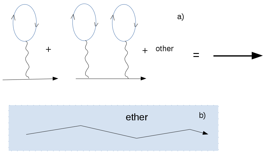
Figure 1: Illustration of vacuum influence on the particle propagation in (a) QFT, where the vacuum loops renormalize the mass and charge of the particle but do not prevent their free motion, and in (b) QG, where the æther fills space due to the absence of an invariant vacuum state.

II Vacuum State and QG

The notion of a vacuum state originates from the ground state of a quantum oscillator. In QFT, the free fields are decomposed into a set of independent field oscillators by Fourier decomposition. Exited states of the oscillators are treated as particles, i.e., matter (both massive and massless). Introducing the interaction term leads to the renormalization of a particle mass and charge, but a one-particle state remains a one-particle state. Consequently, a one-particle wave packet moves freely with the constant envelope velocity, i.e., with no in vacuo dispersion [16]. That implies that even in the presence of perturbative interaction, one could still introduce a LI vacuum state in QFT.

Quantization of GR is too complicated to discuss a vacuum state. Nevertheless, let us consider a toy QG model regarding this issue. In this model only a spatially nonuniform scale factor represents gravity $a(\eta,\bm{r})$. It is certainly not a self-consistent approach within the GR frameworks [17]. Nevertheless, there exists a (1+1)– dimensional toy model [17] including a scalar fields $\bm{\phi}(\tau,\sigma)=\{\phi_{1}(\tau,\sigma),\phi_{2}(\tau,\sigma)\dots\}$ and a scale factor $a(\tau,\sigma)$ described by the action

$$S=\int L\,d\tau=\frac{1}{2}\int\left(-a^{\prime 2}+(\partial_{\sigma}a)^{2}+a^{2}\left(\bm{\phi}^{\prime 2}-(\partial_{\sigma}{\bm{\phi}})^{2}\right)\right)d\sigma d\tau,$$ (1)

where $\tau$ is a time variable, $\sigma$ is a spatial variable, and prime denotes differentiation with respect to $\tau$. Here, like GR, the scalar fields evolve on the curved background $a(\tau,\sigma)$, which is, in turn, determined by the fields. The equations of motion is written as

$$\bm{\phi}^{\prime\prime}-\partial^{2}_{\sigma}\bm{\phi}+2\alpha^{\prime}\bm{\phi}^{\prime}-2\partial_{\sigma}\alpha\partial_{\sigma}\bm{\phi}=0,~{}~{}~{}~{}~{}~{}~{}~{}~{}~{}~{}~{}~{}~{}~{}~{}~{}~{}$$ (2)

$$\alpha^{\prime\prime}-\partial^{2}_{\sigma}\alpha+\alpha^{\prime 2}-(\partial_{\sigma}\alpha)^{2}+\bm{\phi}^{\prime 2}-(\partial_{\sigma}\bm{\phi})^{2}=0.$$ (3)

The relevant Hamiltonian and momentum constraints, written in terms of momentums $\bm{\pi}(\tau,\sigma)\equiv\frac{\delta L}{\delta{\bm{\phi}^{\prime}(\tau,\sigma)}}=a^{2}\bm{\phi}^{\prime}$, $p_{a}(\tau,\sigma)\equiv-\frac{\delta L}{\delta a^{\prime}(\tau,\sigma)}=a^{\prime}$ is

$$\mathcal{H}=\frac{1}{2}\left(-p_{a}^{2}+\frac{\bm{\pi}^{2}}{a^{2}}+a^{2}(\partial_{\sigma}{\bm{\phi}})^{2}-(\partial_{\sigma}a)^{2}\right)=0,$$ (4)

$$\mathcal{P}=-p_{a}\partial_{\sigma}a+\bm{\pi}\partial_{\sigma}\bm{\phi}=0,$$ (5)

and obey the constraint evolution similar to GR [17]:

$$\partial_{\tau}{\mathcal{H}}=\partial_{\sigma}{\mathcal{P}},$$ (6)

$$\partial_{\tau}{\mathcal{P}}=\partial_{\sigma}{\mathcal{H}}.$$ (7)

II.1 Quasi-Heisenberg Quantization and a Region of Small Scale Factor: Absence of Vacuum State

It is believed that our universe originates from a singularity in which a scale factor equals zero. Let us consider a region of small scale-factors first. In this region, it is convenient to use the quasi-Heisenberg picture [18], in which the setting of the initial conditions for operators at the initial moment allows quantization of the equations of motion. In the vicinity of small-scale factors, kinetic energy terms dominate over potential ones [17, 18] so that the equations of motion (2) and (3) reduce to

$$\hat{\bm{\phi}}^{\prime\prime}+2\hat{\alpha}^{\prime}\hat{\bm{\phi}}^{\prime}\approx 0,~{}~{}$$ (8)

$$\hat{\alpha}^{\prime\prime}+\hat{\alpha}^{\prime 2}+\hat{\bm{\phi}}^{\prime 2}\approx 0.$$ (9)

The solutions of Equations (8) and (9) for two scalar fields $\phi_{1}(\tau,\sigma)$, $\phi_{2}(\tau,\sigma)$ under initial conditions, discussed in Appendix A, are written as

$$\hat{\phi_{1}}(\tau,\sigma)=-\frac{i}{\pi_{1}}\int_{-\infty}^{\infty}\theta(\sigma-\sigma^{\prime})S\left(k(\sigma^{\prime})\partial_{\sigma^{\prime}}\,\frac{\delta}{\delta k(\sigma^{\prime})}\right)d\sigma^{\prime}+~{}~{}~{}~{}~{}~{}~{}~{}~{}~{}~{}~{}~{}~{}$$

$$\frac{\pi_{1}}{2\sqrt{\pi_{1}^{2}+k^{2}(\sigma)}}\ln\left(1+2e^{-2\alpha_{0}}\sqrt{\pi_{1}^{2}+k^{2}(\sigma)}\,\tau\right),$$

$$\hat{\phi_{2}}(\tau,\sigma)=i\frac{\delta}{\delta k(\sigma)}+\frac{k(\sigma)}{2\sqrt{\pi_{1}^{2}+k^{2}(\sigma)}}\ln\left(1+2e^{-2\alpha_{0}}\sqrt{\pi_{1}^{2}+k^{2}(\sigma)}\,\tau\right),$$

$$\hat{\alpha}(\tau,\sigma)=\alpha_{0}+\frac{1}{2}\ln\left(1+2\,e^{-2\alpha_{0}}\sqrt{\pi_{1}^{2}+k^{2}(\sigma)}\,\tau\right),$$

where the notations are given in the Appendix A.

As one can see, the scalar fields and the logarithm of the scale factor have monotonic behavior with time. It means that there are no oscillators in the vicinity of small-scale factors and no possibility of defining a vacuum state. In this situation, a quantum state is described by the momentum wave packet $C[k(\sigma)]$ as it is discussed in the Appendix A.

The difference in behavior in the vicinity of small-scale factors and at the epoch of the quantum oscillators occurrence was known long ago from analysis of the Wheeler–DeWitt equation solutions for the Gowdy model [19]. Therefore, we simply illustrate this fact in terms of asymptotic solutions of operator equations.

II.2 String-Like Quantization within the Intermediate Region

From the previous subsection one can see that the operator equations of motion are not the oscillator equations in the vicinity of a$\sim$0, which does not allow defining a vacuum state. A question arises: Could we define a vacuum state when the fields begin to oscillate, and quantum oscillators arise? In this region, the fields obey nonlinear wave Equations (2) and (3), which could not be solved analytically. That complicates using the quasi-Heisenberg picture, and to obtain some analytical results, we will use bosonic string quantization [20, 21]. The action (1) could be rewritten in the reparametrization invariant form of a string on the curved background [17]

$$S=\frac{1}{2}\int d^{2}\xi\sqrt{-g}\,g^{\alpha\beta}(\xi)\partial_{\alpha}X^{A}\partial_{\beta}X^{B}G_{A\,B}(X(\xi)),$$ (10)

where $\xi=\{\tau,\sigma\}$, $X^{A}=\{a,\phi_{1},\phi_{2},\dots\}$, and the metric tensors $g_{\mu\nu}$, $G_{A\,B}(X)$ are in the form of

$$g=\left(\begin{array}[]{cc}-N^{2}+N_{1}^{2}&N_{1}\\ N_{1}&1\end{array}\right),~{}~{}~{}~{}~{}~{}~{}~{}~{}~{}~{}~{}~{}~{}~{}G=\left(\begin{array}[]{cccc}1&0&0&\dots\\ 0&-a^{2}&0&\dots\\ 0&0&-a^{2}&\dots\\ \dots&\dots&\dots&\dots\end{array}\right).$$

The particular gauge for the lapse $N=1$ and shift $N_{1}=0$ functions results in (1). The metric tensor $g_{\alpha\beta}(\xi)$ describes an intrinsic geometry of a (1+1)-dimensional manifold, i.e., a (1+1)-dimensional space-time, and it is an analog of the four-dimensional metric of general relativity. $G_{A\,B}(X(\xi))$ represents a geometry of the external space unifying scale factor and scalar fields and has no direct physical meaning here. The system (10) manifests an invariance relative to the reparametrization of the variables $\tau,\sigma$, which is analog of the general coordinate transformation in GR. The transformations of coordinates $\tilde{\tau}=\tilde{\tau}(\tau,\sigma)$, $\tilde{\sigma}=\tilde{\sigma}(\tau,\sigma)$ imply transition to another reference frame for an observer who “lives on a string”.

For obtaining a vacuum state, the key point is fixing the gauge by taking $g_{\mu\nu}$ in the form of Minkowski’s metric by setting $N=1$, $N_{1}=0$, which simplifies the action (10) to the form

$$S=\frac{1}{2}\int d\sigma d\tau G^{AB}\left(-\partial_{\tau}X_{B}\partial_{\tau}X_{A}+\partial_{\sigma}X_{B}\partial_{\sigma}X_{A}\right).$$ (11)

The momentum

$$P^{A}=\frac{\delta S}{\delta(\partial_{\tau}X_{A})}=-\partial_{\tau}X^{A}=-G^{AB}\partial_{\tau}X_{A}$$ (12)

and the variable $X_{A}$ obey the canonical commutation relations

$$[\hat{P}_{A}(\tau,\sigma),\hat{X}_{B}(\tau,\sigma^{\prime})]=iG_{AB}\delta(\sigma-\sigma^{\prime}).$$ (13)

As a zero-order approximation, one may take $G$ to be equal to $\mathcal{G}$, where

$$\mathcal{G}=\left(\begin{array}[]{ccc}1&0&\dots\\ 0&-1&\dots\\ \dots&\dots&\dots\end{array}\right).$$

Then, it could be possible to develop the perturbation theory on $G-\mathcal{G}$. In zero-order, $X_{A}$ satisfies the wave equation

$$\hat{X}_{A}^{\prime\prime}-\partial^{2}_{\sigma}X_{A}=0,$$ (14)

and the commutation relations (13) can be realized using creation and annihilation operators

$$\hat{X}_{A}=\sum_{k=-\infty}^{\infty}\frac{1}{\sqrt{2k}}\left(\mbox{a}_{kA}e^{ik\sigma-i|k|\tau}+\mbox{a}_{kA}^{+}e^{-ik\sigma+i|k|\tau}\right),$$ (15)

$$\hat{P}_{A}=\sum_{k=-\infty}^{\infty}i\sqrt{\frac{k}{2}}\left(-\mbox{a}_{kA}e^{ik\sigma-i|k|\tau}+\mbox{a}_{kA}^{+}e^{-ik\sigma+i|k|\tau}\right),$$ (16)

where $\mbox{a}_{kA}$, $\mbox{a}_{kB}^{+}$ obey

$$[\mbox{a}_{kA},\mbox{a}_{qB}^{+}]=-\mathcal{G}_{AB}\delta_{k,q}.$$ (17)

Thus, only when the gauge is fixed by $N=1$, $N_{1}=0$, it is possible to define a vacuum state by $\mbox{a}_{kA}|0>=0$. This vacuum state is not gauge-invariant because the dynamic variable $X_{A}$ satisfies the wave Equation (14) in only this gauge (and in zero-order on $G-\mathcal{G}$). Moreover, one could see a problem with the definition of the Fock space of quantum states. Actually, Equation (17) leads to $[\mbox{a}_{k0},\mbox{a}_{k0}^{+}]=-1$. That means that the state $\mbox{a}_{k0}^{+}|0>$ has a negative norm $<0|\mbox{a}_{k0}\mbox{a}_{k0}^{+}|0>=-1$. To avoid the negative norms, the string theory uses additional conditions on the physical Fock states $|>$:

$$\hat{\mathcal{L}}_{f}|>=0,$$ (18)

where $\hat{\mathcal{L}}_{f}=\int(\hat{P}_{A}(\tau,\sigma)+\partial_{\sigma}\hat{X}_{A}(\tau,\sigma))^{2}\,f(\sigma)d\sigma$, and $f(\sigma)$ is an arbitrary function. Operators $\hat{\mathcal{L}}_{f}$ obey the Virasoro algebra. It should be noted that the definition of the Virasoro operators includes the normal ordering [20, 21, 22], but it is beyond the concept of our work. If one accepts the feasibility of using the normal ordering, then the vacuum energy problem does not exist at all. However, we intend to refrain from discussing the status of excluding anomalies in the string theory here.

II.3 Towards a Classical Background

In Section II.1, it is shown that there is no vacuum state in the vicinity of a small scale-factor because of an absence of field oscillators. In principle, the quasi-Heisenberg picture could be used for the description of the subsequent evolution, but it could be done only numerically because solving the operator equations with the initial conditions is complicated. Instead, we have used a string-like quantization described in Section II.2. That allows an analytical consideration of the vacuum state, but it is only half of the problem because a further investigation of the perturbation series on $G-\mathcal{G}$ is needed. Moreover, the trouble with the negative norm of the states can be solved based on the Virasoro algebra by the transition to the $D=26$ dimension in the string theory [20, 21, 22]. The general conclusion for us is that the vacuum state is not gauge-invariant and is defined in a single gauge $N=1$, $N_{1}=0$. We could not make some other physical predictions for this region. However, one could put forward a hypothesis that in the presence of multiple scalar fields, a scale factor acquires monotonic behavior in time and could be considered classically finally. Such a situation is studied in the next section and allows for obtaining a number of physical predictions.

III Vacuum Energy Problem as a Criterion for Finding the Preferred Reference Frame

The more straightforward problem is to define the vacuum state on a classical background space-time. Even in this case, the exact vacuum state exists only for some particular space-time. In other cases, the vacuum state has only an approximate meaning [23]. The observer moving with acceleration straightforwardly [24] or circularly [25] in Minkowski’s space-time will detect quanta of the fields. That means that, although an observer could be in a resting coordinate system, the quantum fields are not in a vacuum state.

Nevertheless, a vacuum state could be defined, for example, in the slowly expanding universe, where a solution to the vacuum energy problem could serve as a criterion for choosing a preferred reference frame. The solution implies avoidance of the enormous zero-point energy density of the quantum fields affecting the universe’s expansion. To do this, a class of conformally unimodular (CUM) metrics has been introduced [15]:

$$ds^{2}\equiv g_{\mu\nu}dx^{\mu}dx^{\nu}=a^{2}\left(1-\partial_{m}P^{m}\right)^{2}d\eta^{2}-\gamma_{ij}(dx^{i}+N^{i}d\eta)(dx^{j}+N^{j}d\eta),$$ (19)

where $x^{\mu}=\{\eta,\bm{x}\}$, $\eta$ is a conformal time, $\gamma_{ij}$ is a spatial metric, $a=\gamma^{1/6}$ is a locally defined scale factor, and $\gamma=\det\gamma_{ij}$. The interval (19) is similar formally to the ADM one [26], but the lapse function is taken in the form of $a(1-\partial_{m}P^{m})$, where $P^{m}$ is a three-dimensional vector, and $\partial_{m}$ is a conventional partial derivative.

Using the restricted class of the metrics (19), the theory [15] has been suggested in which the Hamiltonian constraint is not necessarily zero but equals some constant. Such a theory is known as the Five Vectors theory (FVT) of gravity [15], because the interval (19) contains two 3-vectors $\bm{P}$, $\bm{N}$ and, moreover, spatial metric can be decomposed into a set of three triads $\gamma_{ij}=e_{ia}e_{ja}$, where index $a$ enumerates vectors of the triads $\bm{e}_{a}$.

This theory satisfies the strong equivalence principle (EP) because no additional tensor fields appear. Nevertheless, in contrast to GR, where the lapse and shift are arbitrary functions fixing the gauge, the restrictions $\partial_{n}(\partial_{m}N^{m})=0$ and $\partial_{n}(\partial_{m}P^{m})=0$ arise in FVT. The Hamiltonian $\mathcal{H}$ and momentum $\mathcal{P}_{i}$ constraints in the particular gauge $P^{i}=0$, $N^{i}=0$ obey the constraint evolution equations [15]:

$$\partial_{\eta}{\mathcal{H}}=\partial_{i}\left(\tilde{\gamma}^{ij}\mathcal{P}_{j}\right),$$ (20)

$$\partial_{\eta}{\mathcal{P}_{i}}=\frac{1}{3}\partial_{i}{\mathcal{H}},$$ (21)

where $\tilde{\gamma}_{ij}=\gamma_{ij}/a^{2}$ is a matrix with a unit determinant. Equations (20) and (21) admit adding some constant to ${\mathcal{H}}$ and, in the FVT frame, it is not necessary that $\mathcal{H}=0$, but $\mathcal{H}=const$ is also allowed. That solves the problem of the main part of the zero-point energy density.

Let us consider a spatially uniform, isotropic, and a flat universe with the metric

$$ds^{2}=a(\eta)^{2}(d\eta^{2}-d\bm{x}^{2}),$$ (22)

which belongs to a class of (19). Using the Pauli hard cutoff of the 3-momentums $k_{max}$ [30, 31] reduces the zero-point energy density calculated in the metric (22) to

$$\begin{split}\rho_{v}&=\frac{(N_{boson}-N_{ferm})}{4\pi^{2}a^{4}}\int_{0}^{k_{max}}k^{2}\sqrt{k^{2}+a^{2}m^{2}}dk\approx\\ &\frac{(N_{boson}-N_{ferm})}{16\pi^{2}}\biggl{(}\frac{k_{max}^{4}}{a^{4}}+\frac{m^{2}k_{max}^{2}}{a^{2}}+\frac{m^{4}}{8}\left[1+2\ln\left(\frac{m^{2}a^{2}}{4k_{max}^{2}}\right)\right]+\ldots\biggr{)},~{}\end{split}$$ (23)

where, for simplicity, bosons and fermions of equal masses are considered.

The main part of this energy density $\sim\frac{k_{max}^{4}}{a^{4}}$ scales as radiation, and it has to cause an extremely fast universe expansion in the frame of GR. This result contradicts the observations [32]. In our approach, a constant in the Hamiltonian constraint [15] compensates this main part of zero-point energy and makes it unobservable.

The remaining parts in (23) are also huge but assuming the sum rules for masses of bosons and fermions (the condensates should be taken into account, as well) would provide a mutual compensation for these terms [31, 34]. Of course, all spectrum of the particles in nature, including unknown now, should be taken into account. The empirical cutoff of momentums $k_{max}$ is used in (23), with the hope that some fundamental basis will be found for that in the future (e.g., like a noncommutative geometry [35, 36, 37]), and will provide the UV completions of QG without a renormalization.

Equation (19) determines the preferred reference frame ensuring an æther existence and an absence of dipole anisotropy of the cosmic microwave background (CMB) [38]. Otherwise, the question arises: What is the physical foundation of the frame where CMB is in a rest “in tote,” i.e., does not have a dipole component [39]?

IV Cosmological Consequences of Residual Vacuum Energy

Other contributors to the vacuum energy density are the terms depending on the derivatives of the universe expansion rate [40, 41, 34]. Sum rules cannot remove these terms, but they have the correct order of $\rho_{v}\sim M_{p}^{2}H^{2}$, where $H$ is the Hubble constant, and allow explaining the accelerated expansion of the universe. These energy density and pressure are [40, 41, 34]:

$$\rho_{v} =\frac{a^{\prime 2}}{2a^{6}}M_{p}^{2}S_{0},~{}~{}~{}~{}~{}~{}~{}~{}p_{v}=\frac{M_{p}^{2}S_{0}}{a^{6}}\left(\frac{1}{2}a^{\prime 2}-\frac{1}{3}a^{\prime\prime}a\right),$$ (24)

where, $S_{0}=\frac{k_{max}^{2}}{8\pi^{2}M_{p}^{2}}$ is determined by the UV cut-off of the comoving momenta and the reduced Planck mass $M_{p}=\sqrt{\frac{3}{4\pi G}}$ is implied. The energy density and pressure of vacuum (24) satisfy a continuity equation

$$\rho_{v}^{\prime}+3\frac{a^{\prime}}{a}(\rho_{v}+p_{v})=0,$$ (25)

and, in the expanding universe, are related to the equation of state $p_{v}=w\,\rho_{v}$, as Figure 2 (upper panel) illustrates. Using this equation of vacuum state leads to the cosmological Vacuum Fluctuations Domination (VFD) model [42, 40, 41]. According to VFD the universe behavior at early times, when the scale factor was small, is as freely rolling, i.e., without any deceleration or acceleration, but it is accelerated at a late time. The deceleration parameter $q(a)=-\frac{a^{\prime\prime}a}{{a^{\prime}}^{2}}+1$ is shown in Figure 2 (lower panel) [42]. The discovery of an accelerated universe expansion was a big surprise [43]. However, if the above view of a vacuum is true, a stage preceding the acceleration should be Milne-like, i.e., linear in a cosmic time. The Milne-like universes have been much discussed again recently [44, 45, 46, 47, 48, 49, 50].

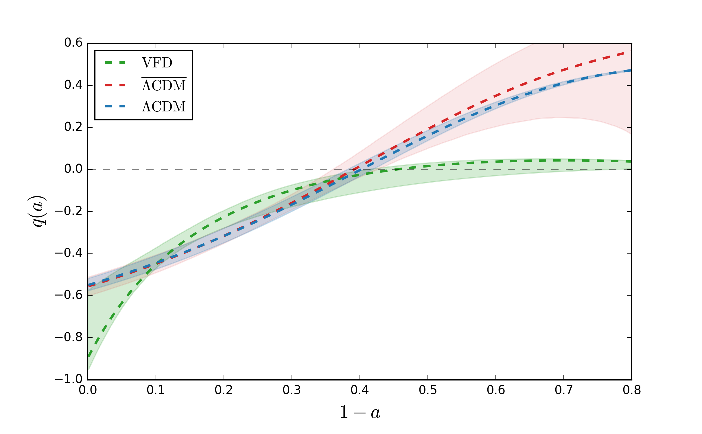
Figure 2: (Upper panel). Equation of the vacuum state in dependence on the universe scale factor $a$. (Lower panel) Deceleration parameter $q(a)$ and the corresponding dispersion channels for the VFD model (24) and two versions of $\Lambda$CDM model.

IV.1 Nucleosynthesis in the Milne-like universe

Nucleosynthesis in a slowly expanding universe was considered earlier [51, 52, 53]. Here, we present our calculation for the VFD model, which has a Milne-like stage, as shown in Figure 2, corresponding to the region where the deceleration parameter $q$ is close to zero. The calculations have been performed with the PRIMAT code (version 0.1.1) [54, 55] including 423 nuclear reactions. The results of the calculations are presented in Table 1 and Figure 3. For comparison, the results for the standard cosmological model are also shown.

As expected, there is a very low rate of neutrons during a period of helium formation in the VFD model (see Figure 3b). That is because an equilibrium between protons and neutrons is shifted towards a neutron decay during the slow universe expansion. Nevertheless, a small amount of neutrons during a long time can create a necessary amount of helium if baryonic density $\Omega_{b}\approx 0.76$. From analysis of Supernovae Type-Ia, Cosmic Chronometers, and Gamma-ray bursts, it was also found that $\Omega_{m}\approx 0.87$ for the VFD model [42]. It means that there is no need for any ad hoc dark matter in the VFD cosmological model because $\Omega_{m}\approx\Omega_{b}$. Moreover, as it was conjectured in [56], spatially nonuniform vacuum polarization should be taken into account in the dynamics of the structure formation.

On the other hand, there is a lot of time for the growth of inhomogeneities in the VFD model [57, 34], and the nonlinear regime begins soon after the last scattering surface. That allows the suggestion that almost all the baryonic matter collapses into eicheons [58], which replace the black holes in FVT. There are no strong constraints on the abundance of black holes in a region of mass $M\sim 10^{13}$– $10^{19}~{}~{}M_{\bigodot}$ [59], and it is possible that the matter concentrates namely in this region.

In the VFD model, there is no cosmological deuterium production. The amount of lithium is less than that in the $\Lambda$CDM, that alleviates the lithium overproduction problem of the standard cosmological model. The amount of CNO is $10^{7}$ times greater compared to $\Lambda$CDM, but it does not contradict the observations [60, 61].

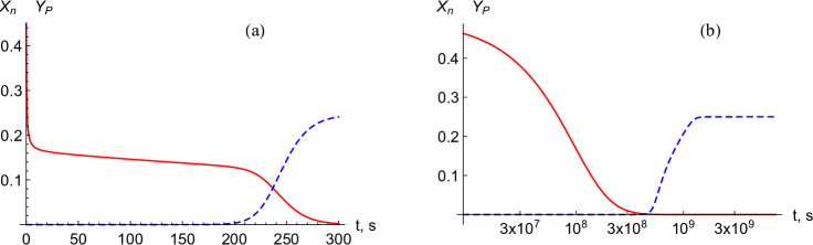
Figure 3: Dependencies of relative abundances of neutron and ${}^{4}\mbox{He}$ on cosmic time $dt=ad\eta$ are given by red and blue curves, respectively, (a) for standard cosmological model, (b) for the VFD model.

Table 1: Final abundances of light elements in the $\Lambda$CDM model at $\Omega_{b}=0.049$ and the VFD model at $\Omega_{b}=0.87$.

	$\Lambda$CDM	VFD
H	0.75	$0.75$
$\mbox{Y}_{p}=4\mbox{Y}_{\mbox{He}}$	$0.25$	$0.25$
$\mbox{D/H}\times 10^{5}$	2.6	$<10^{-25}$
${}^{3}\mbox{He/H}\times 10^{5}$	1.1	$<10^{-8}$
$\mbox{T/H}\times 10^{8}$	7.9	$<10^{-32}$
$(^{7}\mbox{Li}+^{7}\mbox{Be})/\mbox{H}\times{10}^{10}$	5.7	$2.1$
${}^{6}\mbox{Li/H}\times{10}^{14}$	1.2	$<10^{-25}$
${}^{9}\mbox{Be/H}\times{10}^{19}$	9.2	$<10^{-34}$
${}^{10}\mbox{B/H}\times{10}^{21}$	2.9	$<10^{-8}$
${}^{11}\mbox{B/H}\times{10}^{16}$	3.3	$<10^{-10}$
$\mbox{CNO/H}\times{10}^{16}$	8.0	$5.6\times 10^{7}$

It is widely believed that deuterium is produced only cosmologically in $\Lambda$CDM, but for the VFD model, the most plausible and direct way is to create necessary deuterium by beams of antineutrino arising during a collapse [62] before the formation of eicheons in the range of $M\sim 10^{13}$–$10^{19}~{}~{}M_{\bigodot}$. Their formation is unavoidable in the slowly expanding cosmologies because there is much time for the collapse of inhomogeneities in contrast to the standard cosmological model. Indeed, the matter stored in the supermassive eicheons is not related to “dark matter” observed in rotational curves of galaxies because the latter could be explained by the vacuum polarization [56]. Other mechanisms of non-cosmological deuterium production are also discussed [63].

IV.2 Notes about Cosmic Microwave Background in the Slowly Expanding Cosmological Models

By this time, there are no trustable studies of the CMB background for slowly expanding cosmological models, and only some heuristic calculations exist [64]. The main question is the origin of a scale corresponding to the first peak in the CMB spectrum and the origin of the baryon acoustic oscillations (BAO) ruler [65]. In the standard cosmological model, this is the sound horizon’s size at the recombination moment. For the Milne-like cosmology, these quantities must be different [66, 65]. Apart from this, the sound horizon for the Milne-like flat universe is vast and cannot be a scale, which determines the position of the first CMB peak. Let us hypothesize that the width of the last scattering surface [64] could be such a scale for VFD. In this light, the mechanisms of perturbation growth during a recombination period are of interest [67]. As for the BAO ruler, it has to be determined by the complex nonlinear process in the slowly evolving cosmologies and is not related directly to the scale corresponding to the first peak of CMB.

V Size of Eicheon

The concept of æther considered in this work is based on postulating the preferred coordinate frame, namely, CUM. One more consequence of this hypothesis is a replacement of the black hole solutions of GR by the so-called “eicheons”. In Ref. [58], the spherically symmetric solution of the Einstein equations in the CUM metrics (19) was analyzed, and it was found that the finite pressure solution exists for an arbitrarily large mass. As a result, there are no compact objects with an event horizon, because an “eicheon” appears instead of a black hole [58].

In Ref. [58], we have turned from the CUM metrics (27) to Schwarzschild-like in order to demonstrate that a compact object looks like a hollow sphere with a radius greater than that of Schwarzschild (see Figure 4).

Figure 4: (a) A compact object of uncompressible fluid with the radius of $r_{f}$ in the CUM metrics (27) looks as a shell (b) with the boundaries $r_{g}<R_{i}<R_{f}$ in Schwarzschild’s type metric, where $r_{g}$ is a Schwarzschild’s radius.

Here, we intend to calculate the radius of a compact object of constant density in the CUM metrics depending on maximum pressure and density. For a spherically symmetric space-time, the CUM metrics (19) is reduced to

$$ds^{2}=a^{2}(d\eta^{2}-\tilde{\gamma}_{ij}dx^{i}dx^{j})=e^{2\alpha}\left({d\eta^{2}-e^{-2\lambda}(d{\bm{x}})^{2}-(e^{4\lambda}-e^{-2\lambda})({\bm{x}}d{\bm{x}})^{2}/r^{2}}\right),$$ (26)

where $r=|\bm{x}|$ and $\alpha$, $\lambda$ are the functions of $r$. In the spherical coordinates, Equation (26) looks as

$$ds^{2}=e^{2\alpha}\left({d\eta^{2}-dr^{2}e^{4\lambda}-e^{-2\lambda}r^{2}\left({d\theta^{2}+\sin^{2}\theta d\phi^{2}}\right)}\right){\kern 1.0pt}{\kern 1.0pt}.$$ (27)

Let us compare (27) with Schwarzschild’s type metrics

$$ds^{2}=B(R)dt^{2}-A(R)dR^{2}-R^{2}\left({d\theta^{2}+\sin^{2}\theta d\phi^{2}}\right).$$ (28)

The difference between the metrics (26) and (28) is that the metric (28) suggests that the circumference equals $2\pi R$. However, there is no evidence for this fact in an arbitrary spherically symmetric space-time. For the metric (26), the circumference is not equal to $2\pi r$ in the close vicinity of a point-like mass. Coordinate transformation $t=\eta$, $R=R(r)$ relates the metrics (27) and (28), while their comparison gives:

$$B(R)=e^{2\alpha},~{}~{}~{}~{}~{}~{}~{}~{}~{}~{}~{}~{}~{}~{}~{}~{}~{}~{}~{}$$ (29)

$$R^{2}=r^{2}e^{-2\lambda+2\alpha},~{}~{}~{}~{}~{}~{}~{}~{}~{}~{}~{}~{}~{}~{}~{}~{}$$ (30)

$$A(R)\left(\frac{dR}{dr}\right)^{2}=e^{4\lambda+2\alpha}.$$ (31)

Using (29), (30) in (31) to exclude $\lambda$ and $\alpha$ yields

$$\frac{dr}{dR}=\frac{R^{2}}{r^{2}}\frac{A^{1/2}}{B^{3/2}}.$$ (32)

For an empty Schwarzschild space-time $A(R)=(1-r_{g}/R)^{-1}$ and $B(R)=1-r_{g}/R$, whereas in the region filled by matter, $A(R)$ and $B(R)$ obey [72]

$$\frac{d}{dR}\left(\frac{R}{A}\right)=1-\frac{6}{M_{p}^{2}}\rho R^{2},$$ (33)

$$\frac{1}{B}\frac{dB}{dR}=-\frac{2}{p+\rho}\frac{dp}{dR},$$ (34)

where $r_{g}=\frac{3m}{2\pi M_{p}^{2}}$. Further, as in [58], we will consider a model of the constant density $\rho(R)=\rho_{0}$. In this case, Equations (33) and (34) can be integrated explicitly that gives

$$A=\frac{R}{R-r_{g}-2\rho_{0}\left(R^{3}-R_{f}^{3}\right)M_{p}^{-2}},$$ (35)

$$B=\left(1-\frac{r_{g}}{R_{f}}\right)\frac{\rho_{0}^{2}}{(p(R)+\rho_{0})^{2}}$$ (36)

and one needs only to find a pressure $p(R)$, which obeys the Tolman–Volkov–Oppenheimer (TVO) equation

$$p^{\prime}(R)=-\frac{3}{4\pi M_{p}^{2}R^{2}}\mathcal{M}(R)\rho(R)\left(1+\frac{4\pi R^{3}p(R)}{\mathcal{M}(R)}\right)\left(1+\frac{p(R)}{\rho(R)}\right)\left(1-\frac{3\mathcal{M}(R)}{2\pi M_{p}^{2}R}\right)^{-1}.$$ (37)

It is convenient to measure density and pressure in the units of $M_{p}^{2}r_{g}^{-2}$, so that the mean density of Schwarzschild black hole $\rho_{0}=m/(\frac{4}{3}\pi r_{g}^{3})$ equals $1/2$, while the TOV limit $R_{f}<\frac{9}{8}r_{g}$ gives the value of $\rho_{0}=\frac{1}{2}\left(\frac{8}{9}\right)^{3}\approx 0.35$. As for the eicheon radius in Schwarzschild’s type metric, it equals $R_{f}=\sqrt[3]{R_{i}^{3}+\frac{1}{2\rho_{0}}}$ in the units of $r_{g}$, where $R_{i}$ is an inner radius, which determines maximum pressure. Using

$$\mathcal{M}(R)=\frac{4\pi}{3}\rho_{0}\left({R}^{3}-{R_{i}}^{3}\right),$$ (38)

for solving the TOV equation for pressure, it is possible to find $B$, and then solve (32) with the initial condition $r(R_{i})=0$ and find the eicheon radius $r_{f}=r(R_{f})$ in the CUM metrics.

Let us plot (see Figure 5) the calculated radius of the eicheon in the CUM metrics in dependence on density $\rho_{0}$ and maximum pressure, that is, the pressure in the center of a solid ball in the metric (27). An approaching $R_{i}$ to unity increases the maximal pressure. Actual density and pressure in the center of eicheon are defined by the extremal equation of state, which is the subject of future investigations. However, Figure 5 allows concluding that the pressure is considerably smaller than the energy density in a region of interest. That results in a straightforward analytic estimation of the eicheon radius. For the estimation, one could take pressure equal to some constant (e.g., $p(R)=\rho_{0}/10$) in (36), or even simply $p(R)=0$. Then one could take $R_{i}=1$, i.e., the Schwarzschild radius and integrate (32) to obtain

$$r_{f}=\sqrt[3]{3\int_{1}^{R_{f}}\frac{A^{1/2}}{B^{3/2}}R^{2}dR}\approx\frac{\sqrt{3}\sqrt[3]{11}\,\rho_{0}^{1/6}}{2^{5/6}},$$ (39)

where a small “thickness” of the eicheon surface $R_{f}-1$ is used, $R_{f}$ is expressed as $R_{f}=\sqrt[3]{1+\frac{1}{2\rho_{0}}}$ , and only asymptotic term of large $\rho_{0}$ is retained. In the ordinary units, the result reads

$$r_{f}=\frac{3\ 3^{5/6}\sqrt[3]{11}\,m^{4/3}\sqrt[6]{\rho_{0}}}{4\sqrt[6]{2}\,\pi^{4/3}M_{p}^{3}}$$ (40)

and it is slightly unexpected because the eicheon radius rises with the density that turns out to be a specific manifestation of the CUM geometry. In particular, the eicheon of the Planck density $\rho_{0}=M_{p}^{4}$, which is sometimes considered as a maximal density in nature [74] has a radius of $r_{f}\approx 0.8\frac{1}{M_{p}}\left(\frac{m}{M_{p}}\right)^{4/3}$ in the CUM metrics. Looking at the last equation, one may assume that the large eicheons cannot be very dense. However, $r_{f}$ given by (39) is not a physical distance but only points out a border of eicheon in the CUM metrics, whereas the physical distance is given by $l_{eiche}=\int_{0}^{r_{f}}e^{\alpha+2\lambda}dr=\int_{1}^{R_{f}}A^{1/2}dR\approx\frac{5}{24\rho_{0}}$.

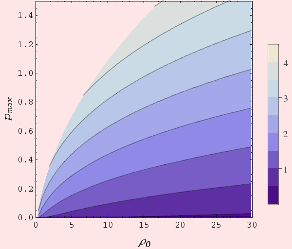
Figure 5: Dependence of the eicheon radius $r_{f}=r(R_{f})$ in the CUM metrics, expressed in the units of gravitational radius, on the density and maximal pressure (i.e., pressure in the eicheon center). Pressure and density are in the units of $M_{p}^{2}r_{g}^{-2}$.

Recently, many investigations explored the footprints of black holes manifesting themselves through star trajectories and a shadow in the accretion disks around the galaxy centers, gravitational lensing, and gravitational waves from the colliding compact objects (see footnote 3 on p. 15). These phenomena can be explained from the properties of both stationary and non-stationary metrics of Schwarzschild and Kerr types, where the radius of “source” objects is of the order of $r_{g}$. It seems reasonable to interpret these observations in the CUM framework and obtain an actual eicheon radius $r_{f}$ using its equation of state. The most informative study originates from collisions of ultracompact massive objects producing the gravitational waves observed by the existing and developing detectors. At this moment, direct astrophysical observations and, much less, analogous modeling cannot provide decisive evidence, which would rule out some alternative concepts of ultracompact massive objects without a horizon (nevertheless, see [76]). One could suggest that off-horizon properties of an eicheon are the same as for a black hole. However, near-horizon phenomena like gravitation wave emission in black hole collisions could be most informative [71, 77, 78] and the study of these phenomena in the framework of FVT is a matter for the future.

VI Decoherence of the Particles Due to Gravitational Potential Fluctuations

Here, we return to the consideration of a locally defined scale factor as an operator. One more implication of the CUM metrics and æther arises for a gravitational decoherence [79], which is the subject of the table-top quantum gravity experiments. In GR, it would not be possible to say that the vacuum fluctuations under Minkowski’s space-time are small. Actually, for the small vacuum fluctuations, one could turn to the reference system where they are significant. That means the appearance of the so-called gauge waves, which are the consequence of the reference frame choice. By restricting the possible reference systems, it would be possible to reveal the actual vacuum fluctuation influencing the motion of the massive particles. The main fundamental question is: Does a massive particle lose its coherence due to interaction with æther? Under Minkowski’s background, one could write for a locally defined scale factor:

$$a(\eta,\bm{r})=(1+\Phi(\eta,\bm{r})),$$ (41)

According to [79], the correlator of the Fourier amplitudes for the gravitational potential in vacuum $\hat{\Phi}(\eta,\bm{r})=\sum_{\bm{k}}\hat{\Phi}_{\bm{k}}(\eta)e^{i\bm{k}\bm{r}}$ takes the form

$$S(\tau-\eta,k)=<0|\hat{\Phi}_{\bm{k}}^{+}(\eta)\hat{\Phi}_{\bm{k}}(\tau)|0>=\int_{-\infty}^{\infty}\tilde{S}(\omega,k)e^{i\omega(\tau-\eta)}d\omega,$$ (42)

where a spectral function $\tilde{S}(\omega,\bm{q})$ is approximately written as [79]

$$\tilde{S}(\omega,k)\approx\left\{\begin{array}[]{c}\frac{N_{all}}{32\pi^{2}{M_{p}}^{4}},\,q<\omega<2k_{max}\\ 0,\,\,\mbox{otherwise}.\end{array}\right.,$$ (43)

where $N_{all}=N_{boson}+N_{ferm}$ is a number of all degrees of freedom.

For a nonrelativistic massive point particle propagating among the fluctuations of the gravitational potential, the Fokker–Plank equation is:

$$\partial_{\eta}f_{\bm{k}}(\bm{p})+i(E_{{\bm{p}}+{\bm{k}}/2}-E_{{\bm{p}}-{\bm{k}}/2})f_{\bm{k}}(\bm{p})=-i\,K_{1}\,\bm{k}\frac{\partial f_{\bm{k}}}{\partial\bm{p}}+2iK_{2}\,\bm{k}\bm{p}\,\Delta_{\bm{p}}f_{\bm{k}}(\bm{p})+2iK_{3}\,p_{i}k_{j}\frac{\partial^{2}f_{\bm{k}}}{\partial p_{j}\partial p_{i}},~{}~{}$$ (44)

where $f_{\bm{k}}(\bm{p})$ is a Fourier transform of the Wigner function $\tilde{f}(\bm{r},\bm{p})=\sum_{\bm{k}}f_{\bm{k}}(\bm{p})e^{i\bm{k}\bm{r}}$. In the first order on the constants $K_{1}$, $K_{2}$, $K_{3}$ it is possible to write:

$$\int f_{\bm{k}}(\bm{p},\eta)f_{-\bm{k}}(\bm{p},\eta)d^{3}\bm{p}d^{3}\bm{k}\approx 1-(3{K_{1}}+3{K_{2}}+6{K_{3}})\frac{\Gamma^{2}\eta^{2}}{m}.$$ (45)

This means that the interaction with a vacuum produces decoherence manifesting itself in the decreasing of “purity” [79] of a particle state according to (45). From Equation (45), the decoherence time is estimated as

$$t_{dec}\approx\frac{1}{\Gamma}\sqrt{\frac{m}{3{K_{1}}+3{K_{2}}+6{K_{3}}}},$$ (46)

and using the approximate expressions for the constants $K_{1},K_{2},K_{3}$, the decoherence length can be found [79]

$$L_{dec}\approx\frac{4M_{p}}{3\sqrt{3\,N_{all}}\pi\,m}\frac{v}{\Gamma}\,,$$ (47)

where $v$ is a particle velocity, $m$ is a particle mass, $1/\Gamma$ is a localization length of the particle wave packet. That is, a point-like particle of mass $m\sim\frac{4M_{p}\,v}{3\sqrt{3N_{all}}\pi}$ loses coherence at a distance equal to the length of the wave packet $1/\Gamma$. It should be noted that interaction with the æther does not produce a particle scattering because the momentum distribution $f_{0}(\bm{p})$ does not change. Nevertheless, decoherence arises. That is a fundamental result implying Lorentz and Galilean invariance violation because one particle state becomes non-pure quantum state.

The difference in particle propagation in the QG and QFT is illustrated in Figure 1. The æther in QG originates from an absence of an invariant vacuum state. The last is not invariant relatively to the general transformation of coordinates and, in particular relative to the Lorentz transformation when it is considered as a subgroup of the general transformation of coordinates.

As regards the decoherence observation (47), such massive point particles are unknown. A real particle of large mass has a finite size, which restricts momentums transferred by the particle form factor: $q<1/d$, where $d$ is particle size. In this case, the following estimation arises [79]

$$L_{dec}\approx\frac{8\pi(M_{p}d)^{2}}{\sqrt{N_{all}}}\frac{v}{\Gamma}.$$ (48)

This quantity seems very large and unobservable. At the same time, the real particles are not rigid but have internal degrees of freedom and consist of a number of point particles, so more careful investigation is needed. Moreover, other possible fundamental mechanisms of decoherence also need investigation [80].

Recently, a gravitationally induced entanglement has attracted great attention (see e.g., [81, 82, 83, 84, 85]). There is no doubt that the nonrelativistic quantum mechanics holds for any interaction, including gravitational interaction in the form of the second Newton’s law and any weak external gravitational field [86]. It is also no doubt that the gravitational waves of linearized gravity are fully analogous to electromagnetic waves and have to be quantized. Undoubtedly, the second Newton’s law could be interpreted as an exchange by gravitons, like the Coulomb law can be interpreted as an exchange by photons. In contrast, the result (47) seems much less trivial because this fundamental decoherence implies the existence of æther with stochastic properties. Such an æther is absent in quantum electrodynamics due to the existence of the LI vacuum state. Implications of the æther in a photon sector of LI violation [87, 88] have to be investigated.

VII Conclusions

To summarize, the CUM metrics gives a sustained basis for quantum gravity physics, cosmology, and physics of compact astrophysical objects. Although fascinating physics like closed time-like curves [89, 90, 91], time machines [92, 93], wormholes [94], and Hawking radiation [95, 96, 97] are excluded in the CUM metrics, these metrics give a fresh impetus to investigate the real physical phenomena, including the structure formation [34], CMB [64], the structure of ultracompact astrophysical objects, and search for the decoherence QG effects and other QG consequences from the vacuum fluctuations of the gravitational potential. All these phenomena imply to single out the conformally unimodular metrics corresponding to a reference system, where the æther is at rest “in tote”. Certainly, it suggests the æther existence per se. In QG, an æther is not simply some background but a thing that weaves all the physical phenomena into a whole quantum universe.

On the other hand, because black holes are absent in this theory, there is no actual “eraser” of the information in the CUM metrics. In other words, a wave function of some particular quantum system is only mixed to a more general wave function, including vacuum and, finally, all universe, and the universe’s wave function seems not an idealization, but a reality conserving all information without any loss [98].

Appendix A Quasi-Heisenberg Quantization

For simplicity, it is convenient to consider two scalar fields, $\phi_{1}$ and $\phi_{2}$, that correspond to a system with three degrees of freedom, including the logarithm of scale factor $\alpha=\ln a$. As a result, there is only one degree of freedom because the Hamiltonian and momentum constraints allow excluding two of them. Let us discuss a quantum picture of the system (1), (4), and (5). The quasi-Heisenberg picture suggests that one needs to define the commutation relations and initial values for operators at the initial moment and then permit the operator evolution according to the equation of motions. For quantization with the help of the Dirac brackets (see also [99]), one should set two additional gauge fixing conditions corresponding to the Hamiltonian and momentum constraints.

Let us take these conditions as

$$\hat{\alpha}(0,\sigma)=\alpha_{0}=const,$$ (49)

$$\partial_{\sigma}\hat{\pi}_{1}(0,\sigma)=0,$$ (50)

i.e., the logarithm of the scale factor and momentum $\hat{\pi}_{1}(0,\sigma)=\pi_{1}$ are $c$-number constants at the initial moment. Generally, that is some time-dependent gauge, which is known only at an initial moment. Then it is permissible for the commutation relations to evolve.

Dirac brackets could allow calculating the operator commutation relations at the initial moment, but the equivalent receipt is to set

$$\hat{\phi}_{2}(0,\sigma)\equiv\varphi(\sigma),$$ (51)

$$\hat{\pi}_{2}(0,\sigma)\equiv-i\frac{\delta}{\delta\varphi(\sigma)},~{}~{}~{}~{}~{}\hat{\phi}_{2}^{\prime}(0,\sigma)=-i\,e^{-2\alpha_{0}}\frac{\delta}{\delta\varphi(\sigma)}$$ (52)

and express other variables from constraints and gauge conditions to obtain

$$\hat{p}_{\alpha}(0,\sigma)=\sqrt{-\frac{\delta^{2}}{\delta\varphi^{2}(\sigma)}+\pi_{1}^{2}},~{}~{}~{}~{}\hat{\alpha}^{\prime}(0,x)=e^{-2\alpha_{0}}\sqrt{-\frac{\delta^{2}}{\delta\varphi^{2}(\sigma)}+\pi_{1}^{2}},$$ (53)

$$\hat{\phi}_{1}(0,\sigma)=\frac{i}{\pi_{1}}\int_{-\infty}^{\infty}\theta(\sigma-\sigma^{\prime})S\left(\frac{\delta}{\delta\varphi(\sigma^{\prime})}\,\partial_{\sigma^{\prime}}\varphi(\sigma^{\prime})\right)d\sigma^{\prime},$$ (54)

$$\hat{\phi}_{1}^{\prime}(0,\sigma)=e^{-2\alpha_{0}}\pi_{1},$$ (55)

where the symbol $S$ denotes symmetrization of the noncommutative operators, i.e., $S(\hat{A}\hat{B})=\frac{1}{2}(\hat{A}\hat{B}+\hat{B}\hat{A})$ or $S(\hat{A}\hat{B}\hat{C})=\frac{1}{6}(\hat{A}\hat{B}\hat{C}+\hat{B}\hat{A}\hat{C}+\hat{A}\hat{C}\hat{B}+\dots)$ and $\theta(\sigma)$ is a unit step function. Its appearance in (54) is the only nontrivial moment that follows from calculation of the Dirac brackets [100], and we have introduced it here for expressing $\phi_{1}$ from the momentum constraint (5).

The equations of motion (2), (3) should be considered as the operator equations with the initial conditions (49), (51)– (55). The second stage of quantization consists of building the Hilbert space where the quasi-Heisenberg operators act. This stage again begins from the classical Hamiltonian (4) and momentum (5) constraints. The momentum constraint and corresponding gauge condition (50) are resolved relatively the variable $\phi_{1}$ and its momentum $\pi_{1}$. Then, these quantities are substituted to the Hamiltonian constraint, which is then quantized and considered as the Wheeler–DeWitt equation in the vicinity of the small scale factor a$\sim$0, i.e., $\ln a=\alpha\rightarrow-\infty$. In such a way, we come to

$$\left(\frac{\delta^{2}}{\delta\alpha(\sigma)}-\frac{\delta^{2}}{\delta^{2}\varphi(\sigma)}+\pi_{1}^{2}\right)\Psi[\alpha,V]=0,$$ (56)

where it is taken into account that $\pi_{1}$ is some constant. Space of the negative frequency solutions of the equation (56) constitutes the Hilbert space for the quasi-Heisenberg operators.

In the general case, the solution of Equation (56) is of the form of the wave packet

$$\Psi[\alpha,\varphi]=\int C[k]\,e^{\int\left(-i\alpha(\sigma)\sqrt{\pi_{1}^{2}+k^{2}(\sigma)}+ik(\sigma)\varphi(\sigma)\right)d\sigma}\,\mathcal{D}k(\sigma),$$ (57)

where only negative frequency solutions are taken and $\mathcal{D}k(\sigma)$ denotes a functional integration over $k(\sigma)$. The scalar product has a form [101, 18, 17]

$$<\Psi|\Psi>=i\,Z\prod_{\sigma}\int\biggl{(}\Psi^{*}[\alpha,\varphi]{\hat{D}^{-1/2}}(\sigma)\frac{\delta}{\delta\alpha(\sigma)}\Psi[\alpha,\varphi]$$

$$~{}~{}~{}~{}~{}~{}~{}~{}~{}~{}~{}~{}~{}~{}~{}~{}~{}~{}-\left({\hat{D}^{-1/2}}(\sigma)\frac{\delta}{\delta\alpha(\sigma)}\Psi^{*}[\alpha,\varphi]\right)\Psi[\alpha,\varphi]\biggr{)}d\varphi(\sigma),$$ (58)

where $\hat{D}(\sigma)=-\frac{\delta^{2}}{\delta\varphi^{2}(\sigma)}+\pi_{1}^{2}$ and $Z$ is a normalization constant. The infinite product is taken over $\sigma$-points, and to be understood in a formal sense as representing the result of a limiting process based on a lattice in $\sigma$-space. The scalar product (58) is independent of the choice of the hyperplane $\alpha(\sigma)$.

The mean value of an arbitrary operator can be evaluated as

$$<\Psi|\hat{A}[\alpha,-i\frac{\delta}{\delta\varphi(\sigma)},\varphi(\sigma)]|\Psi>=i\,Z\prod_{\sigma}\int\biggl{(}\Psi^{*}[\alpha,\varphi]\hat{A}\,{\hat{D}^{-1/2}}(\sigma)\frac{\delta}{\delta\alpha(\sigma)}\Psi[\alpha,\varphi]$$

$$~{}~{}~{}~{}~{}~{}~{}~{}~{}~{}~{}~{}~{}~{}~{}~{}~{}~{}-\left({\hat{D}^{-1/2}}(\sigma)\frac{\delta}{\delta\alpha(\sigma)}\Psi^{*}[\alpha,\varphi]\right)\hat{A}\,\Psi[\alpha,\varphi]\biggr{)}d\varphi(\sigma)\biggr{|}_{\,\alpha(\sigma)=\alpha_{0}\rightarrow-\infty}.$$ (59)

Let us note that the hyperplane $\alpha(\sigma)=\alpha_{0}$ along which the integration is performed in (59), is the same as it is used as an initial condition for the quasi-Heisenberg operator $\hat{\alpha}$ in (17). In a more convenient momentum representation $\hat{\pi}_{2}(\sigma)=k(\sigma)$, $\hat{\phi}_{2}(\sigma)=i\frac{\delta}{\delta k(\sigma)}$, the wave function $\psi$ is

$${\psi}[\alpha,k]=C[k]\exp\left({-i\int\alpha(\sigma)\sqrt{k^{2}(x)+\pi_{1}^{2}}\,dx}\right).$$ (60)

Then, the mean value of an operator becomes

$$<\psi|\hat{A}[\alpha(\sigma),k(\sigma),i\frac{\delta}{\delta k(\sigma)}|\psi>=~{}~{}~{}~{}~{}~{}~{}~{}~{}~{}~{}~{}~{}~{}~{}~{}~{}~{}~{}~{}~{}~{}~{}~{}~{}~{}~{}~{}~{}~{}~{}~{}~{}~{}~{}~{}~{}~{}~{}~{}~{}~{}~{}~{}~{}~{}~{}~{}~{}~{}~{}~{}~{}~{}$$

$$\int C^{*}[k]e^{-i\int\alpha(\sigma)\sqrt{k^{2}(\sigma)+\pi_{1}^{2}}\,d\sigma}\hat{A}\,e^{i\int\alpha(\sigma)\sqrt{k^{2}(\sigma)+\pi_{1}^{2}}\,d\sigma}C[k]\,\mathcal{D}k(\sigma)\biggl{|}_{\,\alpha(\sigma)=\alpha_{0}\rightarrow-\infty}.$$ (61)

Thus, we have an exact quantization scheme consisting of the Wheeler–DeWitt equation in the vicinity of small scale-factor (56), the operator initial conditions (53) for the equations of motion and the expressions (59) and (61) for calculation of the mean values of operators.

References

- Schaffner [1972] K. F. Schaffner, Nineteenth-Century Aether Theories (Pergamon, NY, 1972).
- Berestetskii et al. [1982] V. B. Berestetskii, L. Landau, E. Lifshitz, and L. P. Pitaevskii, Quantum Electrodynamics (Butterworth-Heinemann, Oxford, 1982).
- Klimchitskaya and Mostepanenko [2006] G. L. Klimchitskaya and V. M. Mostepanenko, Contemp. Phys. 47, 131 (2006).
- Mattingly [2005] D. Mattingly, Liv. Rev. Rel. 8, 1 (2005).
- Dirac [1951] P. A. M. Dirac, Nature 168, 906 (1951).
- Collins et al. [2006] J. Collins, A. Perez, and D. Sudarsky, Lorentz invariance violation and its role in quantum gravity phenomenology (2006), arXiv:0603002 [hep-th] .
- Jacobson [2008] T. Jacobson, Proc. Sci. QG-Ph, 020 (2008).
- Horava [2009] P. Horava, Phys. Rev. D 79, 10.1103/physrevd.79.084008 (2009).
- Nilsson and Czuchry [2019] N. A. Nilsson and E. Czuchry, Phys. Dark Univ. 23, 100253 (2019).
- Nilsson [2020] N. A. Nilsson, Aspects of Lorentz and CPT Violation in Cosmology, Ph.D. thesis, National Centre for Nuclear Research, Otwock-Świerk (2020).
- Tureanu [2013] A. Tureanu, J. Phys.: Conf. Ser. 474, 012031 (2013).
- Cherkas et al. [2002] S. L. Cherkas, K. G. Batrakov, and D. Matsukevich, Phys. Rev. D 66, 10.1103/physrevd.66.065011 (2002).
- Kostelecky and Russell [2011] V. A. Kostelecky and N. Russell, Rev. Mod. Phys. 83, 11 (2011).
- Kostelecky and Mewes [2018] V. A. Kostelecky and M. Mewes, Phys. Lett. B 779, 136 (2018).
- Cherkas and Kalashnikov [2019] S. L. Cherkas and V. L. Kalashnikov, Proc. Natl. Acad. Sci. Belarus, Ser. Phys.-Math. 55, 83 (2019), arXiv:1609.00811 [gr-qc] .
- Amelino-Camelia et al. [1998] G. Amelino-Camelia, J. Ellis, N. Mavromatos, D. V. Nanopoulos, and S. Sarkar, Nature 393, 763 (1998).
- Cherkas and Kalashnikov [2012] S. L. Cherkas and V. L. Kalashnikov, Gen. Rel. Grav. 44, 3081 (2012).
- Cherkas and Kalashnikov [2006] S. L. Cherkas and V. L. Kalashnikov, Grav.Cosmol. 12, 126 (2006), arXiv:0512107 [gr-qc] .
- Mizner [1973] C. W. Mizner, Phys. Rev. D 8, 3271 (1973).
- Green et al. [1987] M. B. Green, J. Schwarz, and E. Witten, Superstring Theory, Vol. 1 (Univ. Press, Cambridge, 1987).
- Kaku [2012] M. Kaku, Introduction to Superstrings (Springer, New York, 2012).
- Kiritsis [2019] E. Kiritsis, String Theory in a Nutshell. (Princeton University Press, Princeton, 2019).
- Anischenko et al. [2009] S. Anischenko, S. Cherkas, and V. Kalashnikov, Nonlin. Phenom. Compl. Syst. 12, 16 (2009), arXiv:0806.1593 [quant-ph] .
- Unruh [1976] W. G. Unruh, Phys. Rev. D 14, 870 (1976).
- Akhmedov and Singleton [2008] E. T. Akhmedov and D. Singleton, JETP Lett. 86, 615 (2008).
- Arnowitt et al. [2008] R. Arnowitt, S. Deser, and C. W. Misner, Gen. Rel. Grav. 40, 1997 (2008).
- Lehmkuhl [2019] D. Lehmkuhl, The equivalence principle(s) (2019).
- Knox [2013] E. Knox, Stud. Hist. Philos. Mod. Phys. 44, 346 (2013).
- Shalyt-Margolin [2021] A. Shalyt-Margolin, Int. J. Theor. Phys. 60, 1858 (2021).
- Pauli [1971] W. Pauli, Pauli Lectures on Physics: Vol 6, Selected Topics in Field Quantization (MIT Press, Cambridge, 1971).
- Visser [2018] M. Visser, Particles 1, 138 (2018), arXiv:1610.07264 [gr-qc] .
- Blinnikov and Dolgov [2019] S. I. Blinnikov and A. D. Dolgov, Phys. Usp. 62, 529 (2019).
- Autermann [2016] C. Autermann, Progr.Part. Nucl. Phys. 90, 125 (2016).
- Cherkas and Kalashnikov [2020a] S. Cherkas and V. Kalashnikov, Nonlin. Phenom. Complex Syst. 23, 332 (2020a), arXiv:1810.06211 [gr-qc] .
- Kowalski-Glikman and Nowak [2003] J. Kowalski-Glikman and S. Nowak, Int. J. Mod. Phys. D 12, 299 (2003).
- Pachol [2013] A. Pachol, J. Phys.: Conf. Ser. 442, 012039 (2013).
- Mir-Kasimov [2017] R. M. Mir-Kasimov, Phys. Part. Nucl. 48, 309 (2017).
- Dodelson [2003] S. Dodelson, Modern Cosmology (Elsevier, Amsterdam, 2003).
- Consoli and Pluchino [2021] M. Consoli and A. Pluchino, Universe 7, 10.3390/universe7080311 (2021).
- Cherkas and Kalashnikov [2007a] S. L. Cherkas and V. L. Kalashnikov, JCAP 01, 028, arXiv:0610148 [gr-qc] .
- Cherkas and Kalashnikov [2008] S. L. Cherkas and V. L. Kalashnikov, in Proc. Int. conf. “Problems of Practical Cosmology”,Saint Petersburg, June 23 - 27, 2008 (2008) pp. 135–140, arXiv:astro-ph/0611795 [astro-ph] .
- Haridasu et al. [2020] B. S. Haridasu, S. L. Cherkas, and V. L. Kalashnikov, Fortschr. Phys. 68, 2000047 (2020), arXiv:1912.09224 .
- Perlmutter [2003] S. Perlmutter, Physics Today 56, 53 (2003).
- Sultana [2016] J. Sultana, MNRAS 457, 212 (2016).
- Klinkhamer and Wang [2019] F. R. Klinkhamer and Z. L. Wang, Instability of the big bang coordinate singularity in a milne-like universe (2019), arXiv:1911.11116 [gr-qc] .
- Wan et al. [2019] H.-Y. Wan, S.-L. Cao, F. Melia, and T.-J. Zhang, Phys. Dark Univ. 26, 100405 (2019).
- John [2019] M. V. John, MNRAS Lett. 484, L35 (2019).
- Manfredi et al. [2020] G. Manfredi, J.-L. Rouet, B. N. Miller, and G. Chardin, Phys. Rev. D 102, 10.1103/physrevd.102.103518 (2020).
- Lewis and Barnes [2021] G. F. Lewis and L. A. Barnes, Publ. Astron. Soc. Aust. 38, e007 (2021).
- Chardin et al. [2021] G. Chardin, Y. Dubois, G. Manfredi, B. Miller, and C. Stahl, Astron. Astrophys. 652, A91 (2021), arXiv:2102.08834 [astro-ph.GA] .
- Batra et al. [2000] A. Batra, D. Lohiya, S. Mahajan, A. Mukherjee, and A. Ashtekar, Int. J. Mod. Phys. D 9, 757 (2000).
- Singh and Lohiya [2018] G. Singh and D. Lohiya, MNRAS 473, 14 (2018).
- Lewis et al. [2016] G. Lewis, L. Barnes, and R. Kaushik, MNRAS 460, stw1003 (2016).
- Pitrou et al. [2019] C. Pitrou, A. Coc, J.-P. Uzan, and E. Vangioni, in Proc. of the 15th Int. Symposium on Origin of Matter and Evolution of Galaxies, Kyoto Univ., July 2–5 2019 (2019) p. 011034, https://journals.jps.jp/doi/pdf/10.7566/JPSCP.31.011034 .
- Pitrou et al. [2021] C. Pitrou, A. Coc, J.-P. Uzan, and E. Vangioni, MNRAS 502, 2474 (2021).
- Cherkas and Kalashnikov [2022a] S. L. Cherkas and V. L. Kalashnikov, Universe 8, 10.3390/universe8090456 (2022a).
- Cherkas and Kalashnikov [2021a] S. L. Cherkas and V. L. Kalashnikov, Vestnik Brest Univ., Ser. Fiz.-Mat. 1, 41 (2021a), arXiv:1810.06211 [gr-qc] .
- Cherkas and Kalashnikov [2020b] S. L. Cherkas and V. L. Kalashnikov, Phys. Scr. 95, 085009 (2020b).
- Carr and Kuhnel [2022] B. Carr and F. Kuhnel, SciPost Physics Lecture Notes 10.21468/scipostphyslectnotes.48 (2022).
- Cassisi and Castellani [1993] S. Cassisi and V. Castellani, Astrophys. J. Suppl. 88, 509 (1993).
- Coc et al. [2014] A. Coc, J.-P. Uzan, and E. Vangioni, JCAP 2014, 050.
- Woosley [1977] S. Woosley, Nature 269, 42 (1977).
- Jedamzik [2002] K. Jedamzik, Planetary and Space Science 50, 1239 (2002).
- Cherkas and Kalashnikov [2018] S. L. Cherkas and V. L. Kalashnikov, in Fractional Dynamics, Anomalous Transport and Plasma Science, edited by C. H. Skiadas (Springer, Cham, 2018) Chap. 9.
- Fujii [2020] H. Fujii, Research Notes of the AAS 4, 72 (2020).
- J. et al. [2016] E. J., A., S. Escoffier, O. Le Fèvre, S. Ilić, A. Pisani, S. Plaszczynski, Z. Sakr, V. Salvatelli, T. Schücker, A. Tilquin, and J.-M. Virey, Phys. Rev. D 94, 10.1103/physrevd.94.103511 (2016).
- Lewis [2007] A. Lewis, Phys. Rev. D 76, 10.1103/physrevd.76.063001 (2007).
- Gillessen et al. [2009] S. Gillessen, F. Eisenhauer, S. Trippe, T. Alexander, R. Genzel, F. Martins, and T. Ott, Astrophys. J. 692, 1075 (2009).
- Akiyama et al. [2021] K. Akiyama et al., Astrophys. J. Lett. 910, L12 (2021).
- Abbott et al. [2016] B. P. Abbott et al., Phys. Rev. Lett. 116, 241102 (2016).
- Konoplya and Zhidenko [2016] R. Konoplya and A. Zhidenko, Phys. Lett. B 756, 350 (2016).
- Weinberg [1972] S. Weinberg, Gravitation and Cosmology: Principles and Applications of the General Theory of Relativity (John Wiley & Sons, New York, 1972).
- Lattimer and Prakash [2001] J. M. Lattimer and M. Prakash, Astrophys. J. 550, 426 (2001).
- Barrau and Rovelli [2014] A. Barrau and C. Rovelli, Phys. Lett. B 739, 405 (2014).
- Sandin [2007] F. Sandin, in How And Where To Go Beyond The Standard Model (World Scientific, 2007) pp. 411–420.
- Bambi et al. [2017] C. Bambi, A. Cárdenas-Avendaño, T. Dauser, J. A. García, and S. Nampalliwar, Astrophys. J. 842, 76 (2017).
- Agullo et al. [2021] I. Agullo, V. Cardoso, A. del Rio, M. Maggiore, and J. Pullin, Phys. Rev. Lett. 126, 041302 (2021).
- Dong and Stojkovic [2021] R. Dong and D. Stojkovic, Phys. Rev. D 103, 024058 (2021).
- Cherkas and Kalashnikov [2021b] S. L. Cherkas and V. L. Kalashnikov, Phys. Scr. 96, 115001 (2021b), arXiv:2012.02288 [gr-qc] .
- Petruzziello and Illuminati [2021] L. Petruzziello and F. Illuminati, Nat. Commun. 12, 4449 (2021).
- Belenchia et al. [2018] A. Belenchia, R. M. Wald, F. Giacomini, E. Castro-Ruiz, C. Brukner, and M. Aspelmeyer, Phys. Rev. D 98, 126009 (2018).
- Carney [2022] D. Carney, Phys. Rev. D 105, 024029 (2022).
- Danielson et al. [2022] D. L. Danielson, G. Satishchandran, and R. M. Wald, Phys. Rev. D 105, 086001 (2022).
- Christodoulou et al. [2022] M. Christodoulou, A. Di Biagio, M. Aspelmeyer, C. Brukner, C. Rovelli, and R. Howl, Locally mediated entanglement through gravity from first principles (2022), arXiv:2202.03368 [quant-ph] .
- Krisnanda et al. [2020] T. Krisnanda, G. Y. Tham, M. Paternostro, and T. Paterek, npj Quantum Information 6, 1 (2020).
- Gorbatsievich [1985] A. K. Gorbatsievich, Quantum Mechanics in General Relativity Theory: Basic Principles and Elementary Applications (BSU, Minsk, 1985).
- Martinez-Huerta et al. [2020] H. Martinez-Huerta, R. G. Lang, and V. de Souza, Symmetry 12, 10.3390/sym12081232 (2020).
- Wei and Wu [2021] J.-J. Wei and X.-F. Wu, Tests of lorentz invariance (2021), arXiv:2111.02029 [(astro-ph.HE] .
- Gonzalez-Diaz and Garay [2002] P. Gonzalez-Diaz and L. Garay, in Recent Developments in General Relativity, edited by R. Cianci, R. Collina, M. Francaviglia, and P. Fre (Springer, Genoa, 2002) pp. 459–463.
- Bini and Geralico [2013] D. Bini and A. Geralico, in Eur. Phys. J. Web of Conferences, Eur. Phys. J. Web of Conferences, Vol. 58 (2013) p. 01002.
- Faizuddin [2016] A. Faizuddin, Progr. Phys. 12, 329 (2016).
- Novikov [1989] I. Novikov, JETP 95, 439 (1989).
- Wuthrich [2019] C. Wuthrich, Time travelling in emergent spacetime (2019), arXiv:1907.11167 [physics.hist-ph] .
- Teo [1998] E. Teo, Phys. Rev. D 58, 10.1103/physrevd.58.024014 (1998).
- Herrero-Valea et al. [2021] M. Herrero-Valea, S. Liberati, and R. Santos-Garcia, JHEP 2021 (4), 1.
- Coogan et al. [2021] A. Coogan, L. Morrison, and S. Profumo, Phys. Rev. Lett. 126, 10.1103/physrevlett.126.171101 (2021).
- Saraswat and Afshordi [2021] K. Saraswat and N. Afshordi, JHEP 2021 (2), 1.
- Cherkas and Kalashnikov [2022b] S. L. Cherkas and V. L. Kalashnikov, Nonlin. Phenom. Complex Syst. 25, 266 (2022b), arXiv:1905.06790 [physics.gen-ph] .
- Burdík and Navrátil [2007] C̆. Burdík and O. Navrátil, Univ. J. Phys. Appl. 4, 487 (2007).
- Cherkas and Kalashnikov [2015] S. L. Cherkas and V. L. Kalashnikov, Nonlin. Phenom. Complex Syst. 18, 1 (2015), arXiv:1302.2229 [gr-qc] .
- Cherkas and Kalashnikov [2007b] S. L. Cherkas and V. L. Kalashnikov, in Proc. VIIIth International School-seminar ”The Actual Problems of Microworld Physics”, Gomel, July 25-August 5, Vol. 1 (JINR, Dubna, 2007) p. 208, arXiv:0502044 [gr-qc] .