Comparative Judgement Modeling to Map Forced Marriage at Local Levels

Abstract

Forcing someone into marriage against their will is a violation of their human rights. In 2021, the county of Nottinghamshire, UK, launched a strategy to tackle forced marriage and violence against women and girls. However, accessing information about where victims are located in the county could compromise their safety, so it is not possible to develop interventions for different areas of the county. Comparative judgement studies offer a way to map the risk of human rights abuses without collecting data that could compromise victim safety. Current methods require studies to have a large number of participants, so we develop a comparative judgement model that provides a more flexible spatial modelling structure and a mechanism to schedule comparisons more effectively. The methods reduce the data collection burden on participants and make a comparative judgement study feasible with a small number of participants. Underpinning these methods is a latent variable representation that improves on the scalability of previous comparative judgement models. We use these methods to map the risk of forced marriage across Nottinghamshire thereby supporting the county’s strategy for tackling violence against women and girls.

Keywords: Bradley–Terry Model, Bayesian Inference, Scheduling, Violence Against Women and Girls

1 Introduction

Our work is motivated by a project to estimate the risk of forced marriage across the county of Nottinghamshire, UK. Forced marriage is crime where one or both parties do not consent to the marriage and where pressure or abuse is used to force them into the marriage. It is a form of domestic abuse and a serious abuse of human rights, according to the UK Government, and is illegal under the Anti-social Behaviour, Crime and Policing Act (2014).

Local level data allows the development of targeted safeguarding interventions and policies; however, there is no publicly available data at such a level. The UK Parliament’s Home Affairs Committee’s inquiry into honour-based violence and forced marriage found the lack of data makes it difficult to “formulate policy responses” to honour-based abuse and forced marriage (Home Affairs Commmittee,, 2008). Bates, (2020) argues that identification of victims in a community should be a priority for safeguarding professionals. Previous studies have shown local level policy on forced marriage in the UK is patchy, with procedures varying across local authorities (Chantler et al.,, 2021). The UK Government’s Forced Marriage Unit is a specialised unit devoted to supporting victims, and produces some statistics. They typically deal with over 1,300 cases a year (Forced Marriage Unit,, 2019), but the Unit only provides spatial statistics at regional, not local, level.

Motivated by the need to estimate local level risk of forced marriage in Nottinghamshire, we wish to analyse data on forced marriage at local level in the county. However, there is no centralised database of forced marriage cases in the county. Additionally, victims are supported by a range of independent services (e.g. law enforcement, social services, voluntary agencies), so no one service has a complete picture of the issue. Obtaining data-sharing agreements with all these services would be complex and time consuming. Instead, we carry out a comparative judgement study as this allowed us to collect evidence from a wide range of service providers in the county in an efficient and low cost manner.

Existing comparative judgement models make use of spatial information in a limited way, as a form of prior correlation (Seymour et al.,, 2022) and the interpretation of the results is not straightforward. Instead we develop a method that clusters areas by geolocation and rate of forced marriage, which provides a risk map for safeguarding professionals in the county. In 2021, the office of the Nottinghamshire Police and Crime Commissioner published a strategy on tackling violence against women and girls; the strategy identifies forced marriage as a key crime (Office of the Police and Crime Commissioner in Nottinghamshire,, 2021). One of the aims of the strategy is to work “within the strategic assessments of local partnerships” to tackle violence against women and girls and our clustering method can be used to inform local partnerships.

The pool of potential judges in Nottinghamshire numbers in the tens, whereas previous comparative judgement surveys used hundreds of judges (224 in Seymour et al., (2022) and 1,056 in Marshall, (2020)). Mechanisms to schedule upcoming comparisons for the comparative judgement have been developed previously, but evaluation of these mechanisms has been limited due to high computational costs and intractability. Graßhoff and Schwabe, (2008) were able to analytically derive an experimental design but only for studies with at most three objects. Effective scheduling methods have been developed for studies where comparisons can be made in rounds, e.g. sporting contests, Glickman and Jensen, (2005); Cattelan et al., (2012). The comparisons can be scheduled after each round based on the information learnt from the previous comparisons. Guo et al., (2018) developed an experimental design but, due to the computational cost, an approximate method for inference has been used. In addition to developing a scalable method for making non-approximate inference for comparative judgement models to data, we make use of prior spatial correlation to effectively schedule comparisons in our study.

To address the need for results to inform local partnerships, we develop a Bayesian spatial clustering model to cluster wards by both geolocation and risk of forced marriage (§2.3). To address the limited pool of judges, we develop an efficient scheduling mechanism in §3. To underpin these developments, we introduce an efficient latent variable Markov Chain Monte Carlo algorithm (§4.1) which enables fast inference. We demonstrate our methods via a simulation study (§5) and describe the results of our study in §6.

1.1 Data Collection

To map risk of forced marriage at a high spatial resolution in Nottinghamshire, we carried out a comparative judgement study in the county. Nottinghamshire is a county in central England, with an approximate population of 750,000. Aside from the city of Nottingham in the south and the Mansfield conurbation in the west, the county is largely rural. The county consists of 76 local authority wards (20 in Nottingham City Council and 56 in Nottinghamshire County Council) – a map of the wards used is shown in Figure 1.

Participants, who we refer to as judges, took part in the study remotely via a web interface we designed; they were shown pairs of wards and asked “which of the pair has a higher rate of forced marriage”. There were able to say if they were not familiar with a ward, in which case the comparison was skipped and the ward was not featured in future comparisons. Judges were also able skip a comparison without a reason. We carried out a stakeholder mapping exercise to identify judges and an emailed all judges with an explanation of the project and a link to the interface. We received ethical approval from the University of Nottingham School of Politics and International Relations ethics committee.

A web interface was developed for this study in Python version 3.9 and makes use of following external python packages; flask (v2.0.2), numpy (v1.22.0), pandas (v1.3.5), geopandas (v0.10.2) and SQLAlchemy (v1.4.29). Additionally, SQLite was used as the backend database during the study to collect and store comparative judgements. Images displayed to users during the assessment were sourced from OpenStreetMap data. It was based on the web interface used in Seymour et al., (2022). An example of the web interface that judges see when participating in the study is shown in Figure 2.

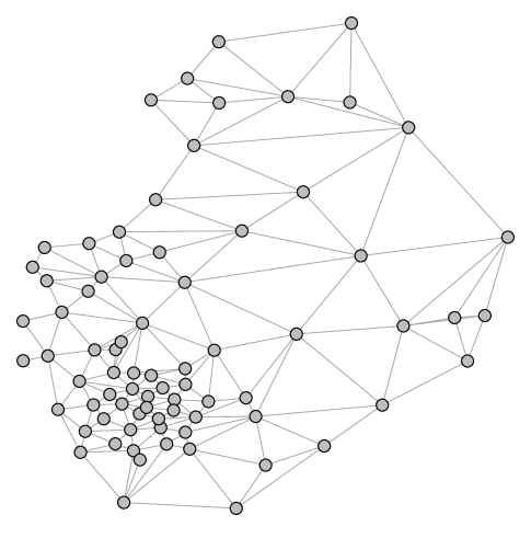
Figure 1: Left: A map of the upper tier local authority wards in Nottinghamshire. Right: The wards represented as a network, nodes represent wards and edges are placed between adjacent wards.

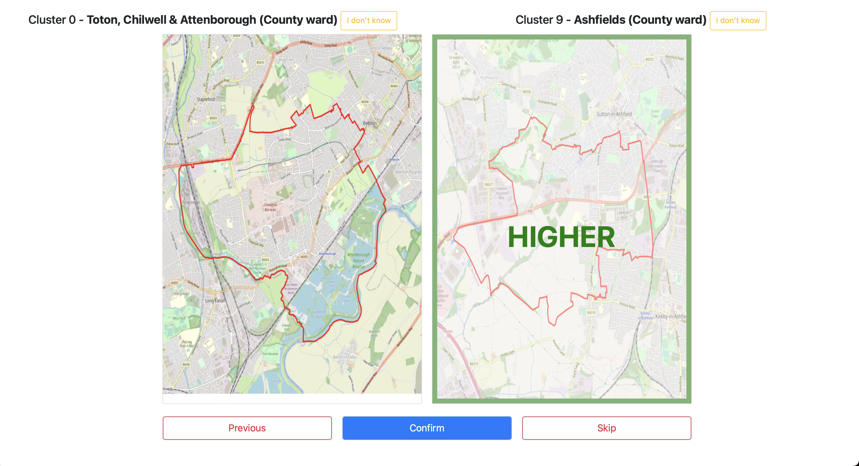
Figure 2: A screenshot of the web interface for the comparative judgement study. Here the judge is asked to compare Toton, Chilwell & Attenborough ward with Ashfields ward. The judge has chosen Ashfields to have the higher rate.

2 Spatial Bradley–Terry Models

2.1 The Standard Bradley–Terry Model

One of the most widely used models for modelling comparative judgement data is the Bradley–Terry model (Bradley and Terry,, 1952) and is defined as follows. Consider a set of wards labelled $1,\ldots,N$. We assign a parameter $\lambda_{i}\in\mathbb{R}$ to each ward describing the (relative) rate of forced marriage; this parameter is sometimes referred to as the quality parameter, but we use the term rate as we asked judges to compare the wards based on rate of forced marriage. For this application, $\lambda_{i}$ is a large positive value if ward $i$ has a high rate of forced marriage and a large negative value if the ward has a low rate of forced marriage. When comparing wards $i$ and $j$, the probability ward $i$ is judged to be have a higher rate than ward $j$ depends on the difference in the rate parameters:

$$\hbox{logit}(\pi_{ij})=\lambda_{i}-\lambda_{j}\iff\pi_{ij}=\frac{\exp(\lambda_{i})}{\exp(\lambda_{i})+\exp(\lambda_{j})}\qquad(i\neq j,1\leq i,j\leq N).$$ (1)

To write the likelihood function for this model, let $n_{ij}$ be the number of times wards $i$ and $j$ are compared, $y_{ij}$ be the number of times ward $i$ is judged to have a higher rate of forced marriage than are $j$ and $\boldsymbol{y}$ the set of outcomes for all pairs of wards. Under the reasonable assumption that comparisons between different pairs of wards and also comparisons for a given pair are independent, the likelihood of the observed data is

$$\pi(\boldsymbol{y}\mid\boldsymbol{\lambda})=\prod_{i=1}^{N}\prod_{j=1}^{i-1}\begin{pmatrix}n_{ij}\\ y_{ij}\end{pmatrix}\pi_{ij}^{y_{ij}}(1-\pi_{ij})^{n_{ij}-y_{ij}},$$ (2)

where $\boldsymbol{\lambda}=\{\lambda_{1},\ldots,\lambda_{N}\}$ is the set of parameters describing the rates for forced marriage. There are a wide variety of methods for estimating the rate parameters, with both classical and Bayesian methods available (Turner and Firth,, 2012; Cattelan et al.,, 2012). As our application has a spatial element, we briefly describe the Bayesian Spatial Bradley–Terry model (BSBT) (Seymour et al.,, 2022).

2.2 The Bayesian Spatial Bradley–Terry Model

The BSBT model allows for the incorporation of prior assumptions about spatial structure of the rate parameters $\boldsymbol{\lambda}$. We place a zero-mean multivariate normal distribution on the rate parameters

$$\boldsymbol{\lambda}\sim\rm MVN(\boldsymbol{0},\Sigma).$$ (3)

To construct the covariance matrix $\Sigma$, we create a network from the wards in the study, treating the wards as nodes and placing edges between adjacent wards. See Figure 1 for the network constructed from the wards in Nottinghamshire. Let $\Lambda=e^{A}$, where $A$ is the adjacency matrix of the network, and $D$ be the matrix containing the diagonal elements of $\Lambda$. The prior distribution covariance matrix is given by

$$\Sigma=\alpha^{2}D^{-\frac{1}{2}}\Lambda D^{-\frac{1}{2}},$$

where $\alpha^{2}$ is a signal variance parameter. Using the matrix exponential assigns high correlation to pairs of wards that are well connected and low correlation to pairs that are only connected via long paths. The normalisation by $D$ ensures the diagonal elements of $\Sigma$ are $\alpha^{2}$ and the off-diagonal entries are proportional to the communicability of each pair of subwards in the network (Estrada and Higham,, 2010). We place a conjugate inverse-Gamma prior distribution on the signal variance parameter $\alpha^{2}$ with shape $\chi$ and scale $\omega$.

The posterior distribution for this model is given by

$$\pi(\boldsymbol{\lambda},\alpha^{2}\mid\boldsymbol{y})\propto\pi(\boldsymbol{y}\mid\boldsymbol{\lambda})\,\pi(\boldsymbol{\lambda}\mid\alpha^{2})\,\pi(\alpha^{2}).$$

2.3 Spatial Clustering Bradley–Terry Model

To address the first limitation we identified and produce results that can align with local partnerships, we now develop a model that clusters the wards by geolocation and rate. It is possible to specify the number of clusters a priori, but it is difficult to justify such a choice. Based on the Bayesian nonparametric method known as a distance dependent Chinese restaurant process (ddCRP) (Blei and Frazier,, 2011), we develop a model where the number of clusters is not specified in advance, but instead learned as part of the statistical inference.

In the spatial clustering BT model, each ward is associated with one other ward (which could be itself) and the clusters are defined implicitly through these associations. The rate parameters $\boldsymbol{\lambda}$ are independently and identically distributed according to an underlying distribution for each cluster. We assume the distribution of the qualities of wards in cluster $k$ is a $N(m_{k},\sigma^{2}_{k})$ distribution, and that there is a base distribution $G_{0}$, according to which the cluster mean and variance parameters are distributed. We take this to be the normal inverse-gamma distribution. We let the assignment of ward $i$ be denoted by $\theta_{i}$, and the prior distribution on the on $\theta_{i}$ is

$$\pi(\theta_{i}=j\mid\beta)\propto\begin{cases}f(i,j)&\textrm{if }i\neq j\\ \beta&\textrm{if }i=j.\\ \end{cases}$$

The concentration parameter $\beta$ controls how likely each ward is to associate with itself, with large values of $\beta$ giving many smaller clusters and small values of $\beta$ giving fewer, larger clusters. The function $f$ determines the probability pairs of wards are associated with each other and is a modelling choice. In our application, we use a distance based metric, $f(i,j)=g(d(i,j))$, based on the graph distance in the network of the wards. The posterior distribution for this model is

$$\pi(\boldsymbol{\lambda},\boldsymbol{\theta},\boldsymbol{m},\boldsymbol{\sigma}^{2}\mid\boldsymbol{y})\propto\pi(\boldsymbol{y}\mid\boldsymbol{\lambda})\,\pi(\boldsymbol{\lambda}\mid\boldsymbol{m},\boldsymbol{\sigma}^{2},\boldsymbol{\theta})\,\pi(\boldsymbol{\theta})\,\pi(\boldsymbol{m}\mid\boldsymbol{\sigma}^{2})\,\pi(\boldsymbol{\sigma}^{2}),$$

where $\boldsymbol{\theta},\boldsymbol{\mu}$ and $\boldsymbol{\sigma}^{2}$ are sets containing the ward assignments, cluster mean and variance parameters respectively.

3 Efficient Data Collection for Spatial Bradley–Terry Models

The second limitation we identified was the limited number of judges. When collecting comparative judgement data about specific abuses or at fine grain levels, there may be a limited number of judges who have sufficient expertise to take part in the study. Therefore, it is particularly important to ask judges to make comparisons that are likely to maximise the information gained in the study. In our motivating example, we are unable to control the number of judges or number of comparisons. Instead, we control the comparisons the judges are asked to make, showing them comparisons that elicit the most information.

In a comparative judgement study, the schedule $\boldsymbol{s}$ is the set of $M$ upcoming comparisons. We focus on schedules where upcoming comparisons are drawn from a distribution, although it is possible to use schedules which are deterministic or manually created. Previous studies have not considered spatial structure when scheduling comparisons. In Seymour et al., (2022) comparisons were scheduled uniformly at random from all possible pairs of wards.

In our motivating study, asking judges to compare two highly connected wards may not elicit the most informative response as we assume the rates are highly correlated. We pursue a scheduling method that utilises the prior covariance structure, with pairs of wards that are not highly connected being prioritised over pairs of wards that are. We derive a probability distribution over all possible comparisons to represent this mechanism. When scheduling comparisons for a study, the pairs of wards are to be compared are drawn from this distribution.

3.1 Scheduling Comparisons for a Spatial Comparative Judgement Study

To construct our scheduling distribution, we adapt a method from principal component analysis to weight the importance of pairs of wards by the amount of prior variance they explain. We denote the distribution by $\mathcal{S}$ and assume $s_{m}\overset{iid}{\sim}\mathcal{S},\,m={1,\ldots,M}$, is the labels of the $m^{th}$ pair of wards to be compared.

As comparisons provide information about one ward relative to another, instead of absolute information, we construct the distribution of difference in the rate parameters. This distribution can be obtained through an affine transformation of the prior distribution $\boldsymbol{\lambda}\sim N(\boldsymbol{\mu},\Sigma)$ and is given by $\boldsymbol{\lambda}_{\rm diff}\sim N(\boldsymbol{\nu},\Delta)$. The vector $\boldsymbol{\lambda}_{\rm diff}=\{\lambda_{1}-\lambda_{2},\lambda_{1}-\lambda_{3},\ldots,\lambda_{N-1}-\lambda_{N}\}$ contains the difference in qualities of each pair of wards, $\boldsymbol{\nu}$ is the corresponding vector of differences in the mean parameters and $\Delta$ is the matrix containing the covariances between each pair of pairs of relative differences. The element of $\Delta$ corresponding to the covariance between the pair $(i,j)$ and $(k,l)$ is given by

$$\hbox{Cov}(\lambda_{i}-\lambda_{j},\lambda_{k}-\lambda_{l})=\hbox{Cov}(\lambda_{i},\lambda_{k})-\hbox{Cov}(\lambda_{i},\lambda_{l})-\hbox{Cov}(\lambda_{j},\lambda_{k})+\hbox{Cov}(\lambda_{j},\lambda_{l}).$$

The spectral decomposition of the covariance matrix $\Delta$ is $\Delta=U\Psi U^{T}$, where $\Psi$ is a diagonal matrix of eigenvalues of $\Delta$ and columns of $U$ are the corresponding eigenvectors. We order the eigenpairs $\{\psi^{(c)},\boldsymbol{u}^{(c)}\}$ such that $\psi^{(c)}\geq\psi^{(c+1)}$ (recall that $\psi^{(c)}\geq 0$ since $\Delta$ is positive semidefinite). The eigenvectors create an orthogonal basis for $\mathbb{R}^{N(N-1)/2}$ and each vector is known as a principal component (Mardia et al.,, 1979).

The $c^{th}$ principal component is the vector that explains the maximum variance of the prior distribution of $\boldsymbol{\lambda}_{\rm diff}$ whilst still being orthogonal to the $c-1$ vectors before it. The proportion of variance explained by the $c^{th}$ principal component is $\frac{\psi^{(c)}}{\sum_{d}\psi^{(d)}}$ and the $i^{th}$ variable in the $c^{th}$ principal component can be thought of as explaining $\frac{\left(\mathbf{u}^{(c)}_{i}\right)^{2}}{\sum_{k}\left(\mathbf{u}^{(c)}_{k}\right)^{2}}$ proportion of this proportion of variability.

We then define the probability pair $\{i,j\}$ is shown to a judge is

$$p_{i,j}=\frac{\sum_{c}\left(\mathbf{u}^{(c)}_{\beta}\right)^{2}\psi^{(c)}}{\sum_{c}\psi^{(c)}},$$

with $\beta=\frac{N(N-1)}{2}-\frac{(N-i+1)(N-i)}{2}+j-i$ being the linear index of $\boldsymbol{\lambda}_{\rm diff}$ corresponding to the pair $(i,j)$. This is equivalent to the sum of the loadings squared for a ward’s rate parameter over the total variance explained. The set $\{p_{1,2},\ldots,p_{N,(N-1)}\}$ describes the probability distribution $\mathcal{S}$ over the set of pairs of wards which places higher mass on pairs which have higher prior variance.

4 Scalable Bayesian Inference for Bradley–Terry Models

We now describe our method to perform posterior computation, a latent variable algorithm. Our latent variable algorithm is considerably more efficient than the currently available algorithms (Seymour et al.,, 2022), providing a better mixing Markov chain and a faster time to convergence. This allows us to evaluate scheduling mechanisms and to implement inference algorithms for the clustering model.

4.1 Pólya-Gamma Latent Variable Representation

We now present an alternative latent variable formulation of the BT model that allows incorporation of a prior covariance structure for the rate parameters $\boldsymbol{\lambda}$ and leads to a very efficient Gibbs sampler; this formulation is based on Caron and Doucet, (2012). Consider the likelihood contribution from all comparisons of the pair of wards $(i,j)$. If this pair is compared $n_{ij}$ times, out of which ward $i$ was judged to be superior to ward $j$ $y_{ij}$ times, then the likelihood contribution is

$$\pi_{ij}(\boldsymbol{\lambda})=\frac{\exp\left(\boldsymbol{x}_{ij}^{T}\,\boldsymbol{\lambda}\right)^{y_{ij}}}{\left(1+\exp\left(\boldsymbol{x}_{ij}^{T}\,\boldsymbol{\lambda}\right)\right)^{n_{ij}}},\quad i,j=1,\ldots,N,$$

where $\boldsymbol{x}_{ij}$ is $N\times 1$ vector with all elements being zero apart from the $i^{\mbox{\tiny{th}}}$ and $j^{\mbox{\tiny{th}}}$ elements which take values $1$ and $-1$ respectively. Introducing a latent variable $z_{ij}$ which follows a Pólya-Gamma distribution and then following Polson et al., (2013) we can write

$$\pi_{ij}(\boldsymbol{\lambda})\propto\exp\left(k_{ij}\,\boldsymbol{x}_{ij}^{T}\,\boldsymbol{\lambda}\right)\int_{0}^{\infty}\exp\left(-z_{ij}\left(\boldsymbol{x}_{ij}^{T}\,\boldsymbol{\lambda}\right)^{2}/2\right)p(z_{ij}|n_{ij},0)\mbox{ d}z_{ij},$$

where $k_{ij}=y_{ij}-n_{ij}/2$ and $p(z_{ij}|n_{ij},0)$ is the density of a Pólya-Gamma random variable with parameters $n_{ij}$ and 0. We can now augment the observed data $\boldsymbol{y}$ from all $M$ pairs of wards with the corresponding set $\boldsymbol{z}=(z_{ij})$ of latent variables for all pairs of wards and write the observed-data likelihood as follows:

$$\pi(\boldsymbol{y}|\boldsymbol{\lambda}) \propto\int_{\boldsymbol{z}}\pi(\boldsymbol{y},\boldsymbol{z}|\boldsymbol{\lambda})\mbox{ d}\boldsymbol{z}=\prod_{i=1}^{N}\prod_{j<i}\pi_{i,j}(\boldsymbol{\lambda})$$

$$=\prod_{i=1}^{N}\prod_{j<i}\Bigg{(}\exp\left(k_{ij}\,\boldsymbol{x}_{ij}^{T}\,\boldsymbol{\lambda}\right)\int_{0}^{\infty}\exp\left(-z_{ij}\left(\boldsymbol{x}_{ij}^{T}\,\boldsymbol{\lambda}\right)^{2}/2\right)p(z_{ij}|n_{ij},0)\mbox{ d}z_{ij}\Bigg{)}.$$ (4)

As in the Exponential latent variable representation in Caron and Doucet, (2012), the introduction of $\boldsymbol{z}$ is instrumental in constructing a scalable and efficient MCMC algorithm. The conditional posterior distributions $\pi(\boldsymbol{z}|\boldsymbol{y},\boldsymbol{\lambda})$ and $\pi(\boldsymbol{\lambda}|\boldsymbol{z},\boldsymbol{y})$ are available in closed form, leading to a straightforward implementation of a Gibbs sampler. Letting $X$ be the BT design matrix constructed from $\boldsymbol{x}_{ij}$, the conditional distribution of $\boldsymbol{\lambda}|\boldsymbol{y},\boldsymbol{z}$ is derived by

$$\pi(\boldsymbol{\lambda}|\boldsymbol{z},\boldsymbol{y}) \propto\pi(\boldsymbol{\lambda})\prod_{i=1}^{N}\prod_{j<i}\pi_{ij}(\boldsymbol{\lambda})$$

$$=\pi(\boldsymbol{\lambda})\prod_{i=1}^{N}\prod_{j<i}\exp\left(k_{ij}\,\boldsymbol{x}_{ij}^{T}\,\boldsymbol{\lambda}-z_{ij}\left(\boldsymbol{x}_{ij}^{T}\,\boldsymbol{\lambda}\right)^{2}/2\right)$$

$$=\pi(\boldsymbol{\lambda})\prod_{i=1}^{N}\prod_{j<i}\exp\left(\frac{z_{ij}}{2}\left(\boldsymbol{x}_{ij}^{T}\,\boldsymbol{\lambda}-\frac{k_{ij}}{z_{ij}}\right)^{2}\right)$$

$$=\pi(\boldsymbol{\lambda})\exp\left(-\frac{1}{2}\left(\boldsymbol{\zeta}-X\boldsymbol{\lambda}\right)^{T}Z(\boldsymbol{\zeta}-X\boldsymbol{\lambda})\right)$$

$$=\pi(\boldsymbol{\lambda})\exp\Bigg{(}-\frac{1}{2}\left(\boldsymbol{\lambda}-X^{-1}\boldsymbol{\zeta}\right)^{T}\left(X^{T}ZX\right)\left(\boldsymbol{\lambda}-X^{-1}\boldsymbol{\zeta}\right)\Bigg{)},$$

where $Z=\mbox{diag}(z_{ij})$ and $\boldsymbol{\zeta}=\left(k_{12}/z_{12}\,,k_{13}/z_{13},\ldots,k_{N-1\,N}/z_{N-1\,N}\right)$. Assigning a multivariate Normal prior distribution on $\boldsymbol{\lambda}$ that allows for a priori dependence among the rate parameters $\boldsymbol{\lambda}$, i.e. $\boldsymbol{\lambda}\sim N(\bar{\boldsymbol{\mu}},{\Sigma})$, it can be shown that

$$\boldsymbol{\lambda}|\boldsymbol{y},\boldsymbol{z}\sim N(\boldsymbol{\mu},S),$$ (5)

where $S=\left(X^{T}ZX+\Sigma^{-1}\right)^{-1}$ and $\boldsymbol{\mu}=S\left(X^{T}\left(\boldsymbol{y}-\boldsymbol{n}/2)\right)+\Sigma^{-1}\bar{\boldsymbol{\mu}}\right)$. By the definition of a Pólya-Gamma random variable and its expectation Polson et al., (2013) shows that

$$\pi(z_{ij}|y_{ij},\lambda_{ij})\sim PG(n_{ij},\lambda_{i}-\lambda_{j}).$$ (6)

Sampling from (6) can be efficiently done using an accept/reject algorithm based on the alternating-series method of Devroye, (1986). In conjunction with exploiting the sparse structure of the matrix $X$, we have a Gibbs sampler in Algorithm 1 that allows sampling of the joint posterior distribution of $\boldsymbol{\lambda}$ and $\boldsymbol{z}$ and which is scalable and efficient to implement.

Algorithm 1 The Pólya-Gamma latent variable algorithm

Initialise the chain with values $\lambda_{1},\ldots,\lambda_{m}$ and $z_{1,2}\ldots z_{N-1,N}$

repeat

     for $1\leq i<j\leq N,n_{ij}>0$ do

         Draw $z_{ij}\sim PG(n_{ij},\lambda_{i}-\lambda_{j})$

     end for

     Draw $\boldsymbol{\lambda}\sim\textrm{MVN}(\boldsymbol{\mu},S)$

     Draw values for any model hyperparameters

until Markov chain has converged

An R software package to implement the MCMC algorithm can be found at https://anonymous.4open.science/r/speedyBBT-B53F/README.md [anonymised for review].

4.2 Spatial Clustering Bradley–Terry Model

The Pólya-Gamma latent variable representation can be used with the spatial clustering model and we now adapt Algorithm 1 to construct an MCMC algorithm for this model. Recall that in the clustering model each ward is assigned to another ward $\theta_{i}$ and $\boldsymbol{\theta}=(\theta_{i})$ define the clustering. When updating $\theta_{i}$ there are three possibilities we need to consider: that $\theta_{i}=i$; that $\theta_{i}=j\neq i$ and this assignment results in two clusters merging; that that $\theta_{i}=j\neq i$ and this connection does not result in two clusters merging. Example configurations are given in Figure 3. The full conditional distribution for $\theta_{i}$ is

$$\pi(\theta_{i}\mid\boldsymbol{\theta}_{-i},\boldsymbol{\lambda}^{*})\propto\begin{cases}\beta&\hbox{if }\theta_{i}=i,\\ f(i,j)\frac{\pi(\boldsymbol{\lambda}_{k}\cup\boldsymbol{\lambda}_{l}|G_{0})}{\pi(\boldsymbol{\lambda}_{k}|G_{0})\pi(\boldsymbol{\lambda}_{l}|G_{0})}&\hbox{if }\theta_{i}=j\hbox{ and clusters }k\hbox{ and }l\hbox{ would be joined},\\ f(i,j)&\hbox{if }\theta_{i}=j\hbox{ and a two clusters would not be joined,}\\ \end{cases}$$

where $\boldsymbol{\theta}_{-i}$ is the set of assignments excluding the assignment for ward $i$, and $\boldsymbol{\lambda}_{k}$ are the rate parameters associated with wards in cluster $k$. The term $\pi(\boldsymbol{\lambda}_{k}|G_{0})$ is the marginal likelihood

$$\pi(\boldsymbol{\lambda}_{k}\mid G_{0}) =\iint\prod_{i;\theta_{i}=k}\pi(\lambda_{i}\mid\mu,\sigma^{2})\,dG_{0}(\mu,\sigma^{2})$$

$$=\iint\left(\prod_{i;\theta_{i}=k}\pi(\lambda_{i};\mu,\sigma^{2})\right)\pi(\mu|\sigma^{2})\pi(\sigma^{2})\,d\mu\,d\sigma^{2}$$

$$=\frac{\Gamma(\alpha_{o}+n_{k}/2)}{\Gamma(\alpha_{0})}\frac{\beta_{0}^{\alpha_{0}}}{\bar{\beta}^{\alpha_{0}+n_{k}/2}}\left(\frac{1}{1+n_{k}}\right)^{\frac{1}{2}}(2\pi)^{-\frac{n_{k}}{2}},$$

where $\bar{\beta}=\beta_{0}+\frac{1}{2}\sum_{i;\theta_{i}=k}(\lambda_{i}-\theta_{k})^{2}+\frac{n_{k}(\theta_{k}-\mu_{0})^{2}}{2(1+n_{k})}$ and $\theta_{k}=\frac{1}{n_{k}}\sum_{i;\theta_{i}=k}\lambda_{i}$.

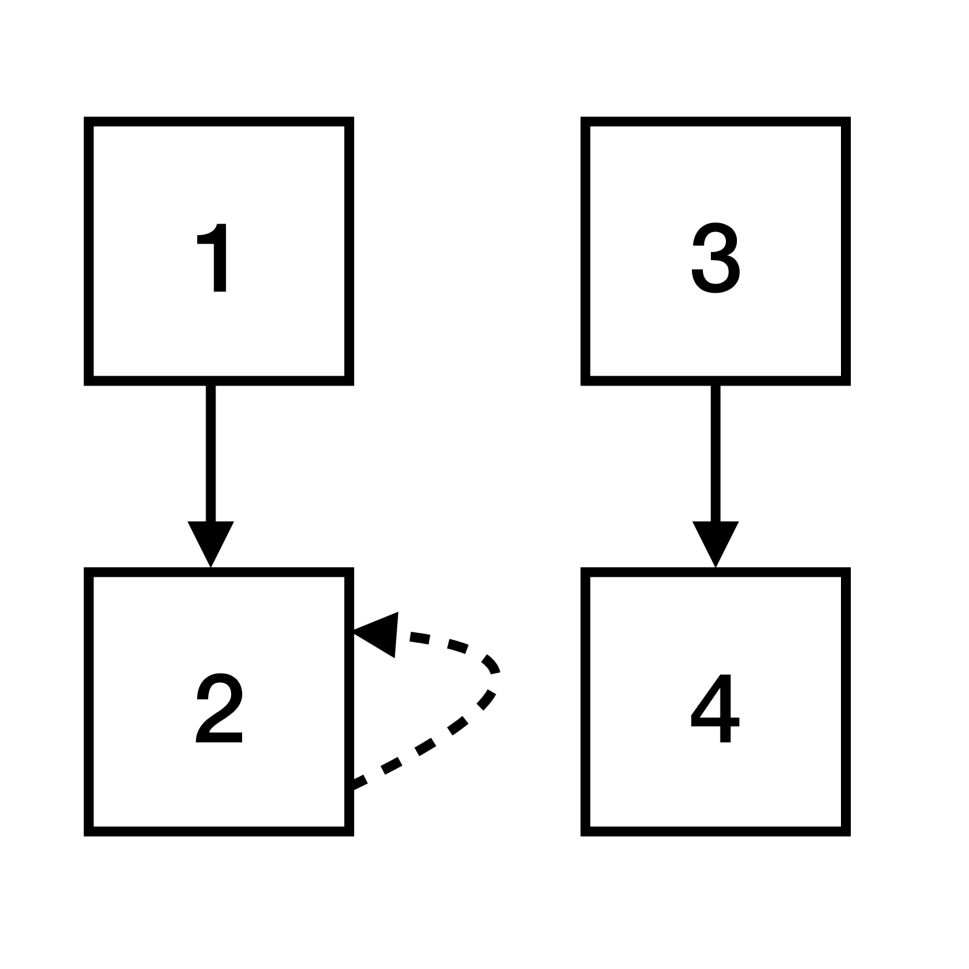
(a) Ward 2 is assigned to itself creating two clusters.

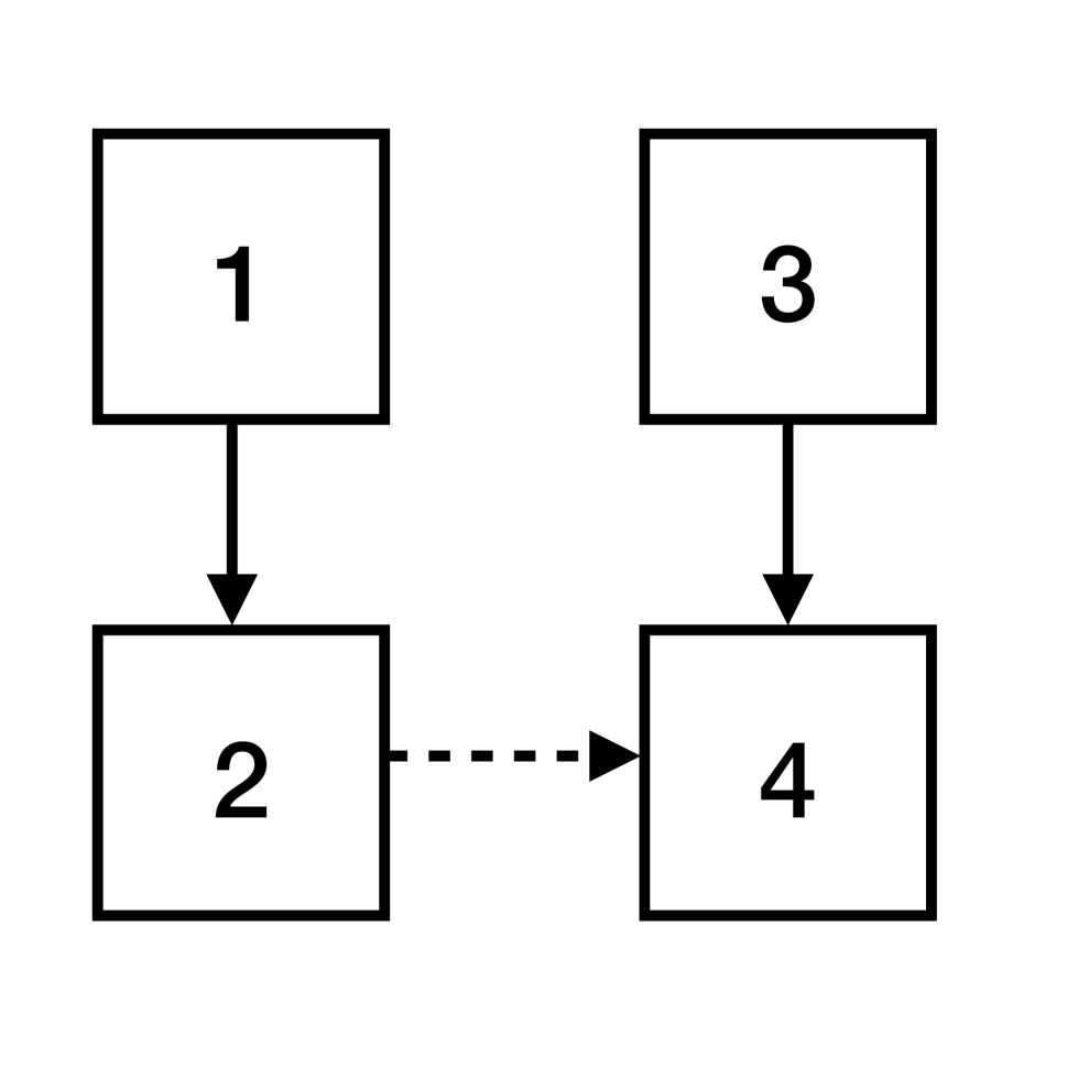
(b) Ward 2 is assigned to ward 4, creating one cluster.

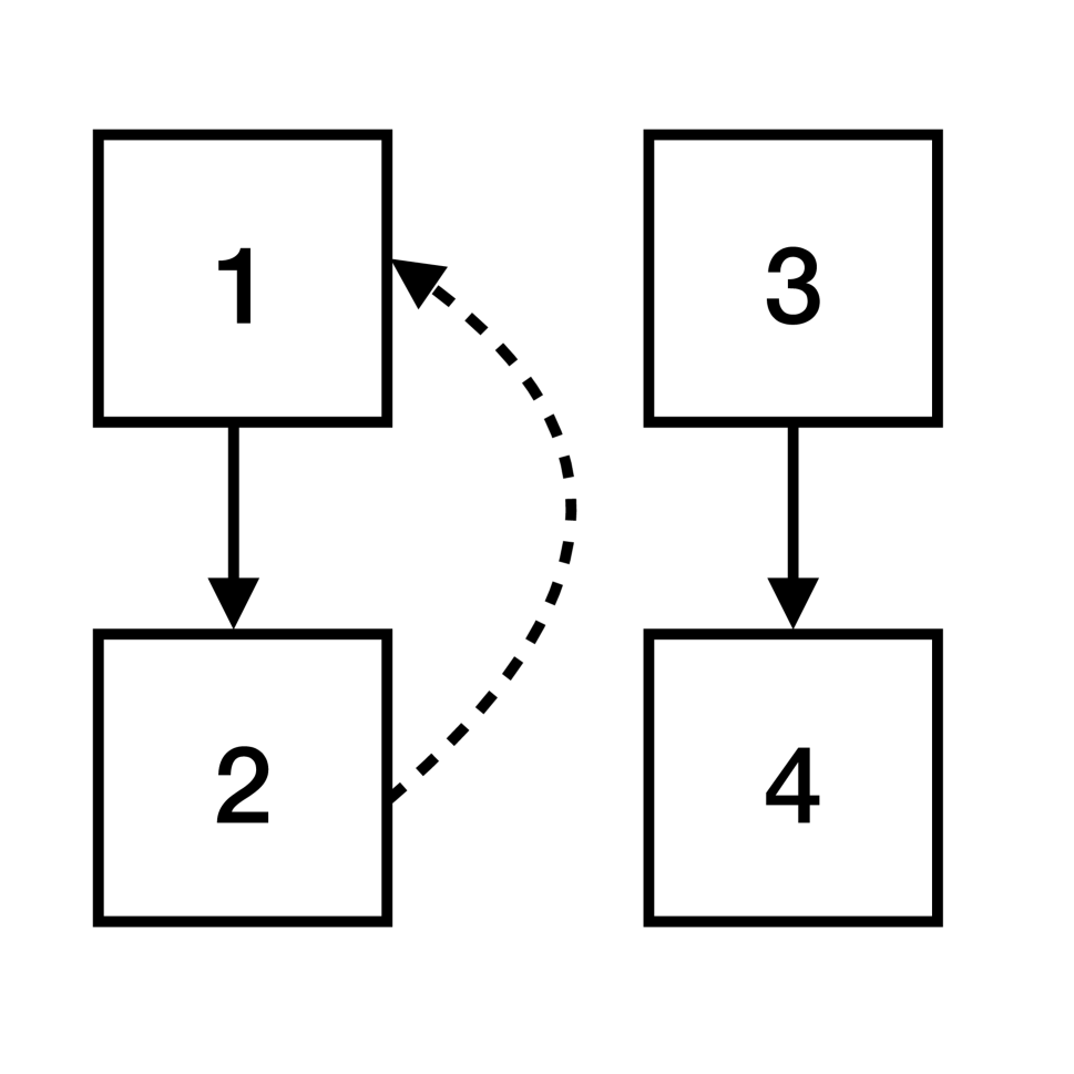
(c) Ward 2 is assigned to ward 1, creating two clusters.

Figure 3: An example of three configurations when assigning ward 2 to another ward. The dashed arrow corresponds to the assignment of ward 2.

We parameterise the cluster variance parameters through their inverses, the cluster precision parameters. The full conditional distribution for the precision of cluster $k$ is

$$\frac{1}{\sigma^{2}_{k}}\mid\boldsymbol{m},\boldsymbol{\lambda},\boldsymbol{\theta}\sim\Gamma\left(\alpha_{0}+\frac{n_{k}}{2},\,\bar{\beta}\right).$$

The full conditional distribution for the mean parameter for cluster $k$, $\lambda_{k}^{*}$, is given by

$$m_{k}|\sigma^{2}_{k},\boldsymbol{\lambda},\boldsymbol{\theta}\sim N\left(\frac{\mu_{0}+n_{k}\theta_{k}}{1+n_{k}},\frac{\sigma^{2}_{k}}{1+n_{k}}\right).$$

4.3 Identifiability

Model (1) is invariant to translations and hence an identifiability constraint is necessary when inferring the rate parameters $\boldsymbol{\lambda}$. This does not change the value of the likelihood function as it is invariant to translations. We adapt the translation in Caron and Doucet, (2012) and define

$$\Lambda=\frac{1}{N}\sum_{i=1}^{N}\lambda_{i}$$

to be the mean of the rate parameters. Under the prior distribution (3) the distribution of $\Lambda$ is

$$\Lambda\sim N\left(0,\frac{\boldsymbol{1}\Sigma\boldsymbol{1}^{T}}{N^{2}}\right),$$

where $\boldsymbol{1}=(1,\ldots,1)^{T}$ is a vector of ones. At each iteration of Algorithm 1 we draw a value for $\Lambda$ and translate the values of $\boldsymbol{\lambda}$.

5 Simulation Study

We now assess the utility of our spatial scheduling mechanism and compare it to two other scheduling mechanisms. The first scheduling mechanism is where pairs of wards are chosen uniformly at random from all possible pairs of wards. The second is a naive spatial scheduling mechanism, where the probability a pair of wards is chosen for comparison depends on how connected they are. Firstly, we construct a vector $\boldsymbol{p}^{*}$, where each element describes the connectedness between a pair of wards, i.e. the matrix $\exp(A)_{ij}$ in vector form. Secondly, we normalise $\boldsymbol{p}^{*}$ to create a probability distribution. The distribution governing the scheduling mechanism is given by

$$\boldsymbol{p}\propto\boldsymbol{1}-\frac{\boldsymbol{p}^{*}}{\sum\boldsymbol{p}^{*}}.$$

We subtract the normalised vector from one to assign low probability to pairs of wards that are highly connected and high probability to pairs of wards that are not.

We simulate 1,000 synthetic sets of rate parameters for the wards in Nottinghamshire. The values for the rate parameters were drawn from the distribution in equation (3) with $\alpha=3$. For each of the sets of rate parameters we simulate three sets of 500 comparisons, each corresponding to one of the three scheduling mechanisms. We choose 500 comparisons, as this represents 10 judges doing 50 comparisons each, which was our target for the data collection activity. We then fit the model to the simulated comparisons using the Pólya-Gamma latent variable representation and running the algorithm for 500 iterations; we remove the first 50 iterations as a burn-in period. For each set of comparisons we record the utility of the scheduling mechanism. Running such a large number of simulations is only possible using the Pólya-Gamma latent variable representation,

To assess the effectiveness the schedules, we define the utility of the schedule. There are a wide range of utility functions (see, e.g., Ryan et al.,, 2015), but due to the identifiability issues in the BT model, our choice of utility function is limited. We define the utility of a schedule $\boldsymbol{s}\in\mathcal{S}$ given the comparisons $\boldsymbol{y}$ to be

$$U(\boldsymbol{s}\mid\boldsymbol{y})=\frac{1}{\textrm{tr}(\textrm{cov}(\boldsymbol{\lambda}\mid\boldsymbol{s},\boldsymbol{y}))},$$

where $\textrm{cov}(\boldsymbol{\lambda}\mid\boldsymbol{s},\boldsymbol{y})$ is the posterior covariance matrix of the parameters $\boldsymbol{\lambda}$. This is referred to as the Bayesian A-posterior precision utility function and it depends on the variances of the marginal posterior distribution of the rate parameters (Ryan et al.,, 2015).

Table 1 summarises the utility across all 5,000 sets of comparisons. The principal component based scheduling mechanism has a greater utility than either of the other two deigns, with the mean utility for this scheduling mechanism around five times higher than for the two simpler scheduling mechanisms. The principal component scheduling mechanism allows for more information to be gained from fewer comparisons, and, on average, provides a 13% increase in the utility of the scheduling mechanism. Despite taking the spatial structure into account, the naive spatial scheduling mechanism has the same utility as the uniform scheduling mechanism, evidencing the effectiveness of our new spatial scheduling mechanism at gaining information from judges.

Table 1: The mean, minimum, and maximum utility for the three scheduling mechanisms across 5,000 simulated data sets.

Scheduling mechanism	Mean	Minimum	Maximum
Uniform	0.199	0.106	0.256
Naive spatial	0.197	0.108	0.257
Principal component	0.224	0.116	0.292

Two further simulation studies comparing the efficiency of MCMC algorithms are presented in the Supplementary Material

6 Forced Marriage in Nottinghamshire

There are a limited number of individuals with sufficient expertise in forced marriage in Nottinghamshire to act as judges in this study, and this was our motivation to develop a method to maximise the information gained from each comparison. We identified 29 organisations supporting victims of forced marriage in the county, this included large organisations such as local authorities and small organisations, such as charities run by volunteers. The organisations were identified through a stakeholder mapping exercise and through the Nottinghamshire modern slavery partnership (forced marriage has been included as a form of modern slavery by the International Labour Organisation since 2017).

Invites to take part in the study were emailed to individuals from all 29 organisations identified. We recruited 12 judges who made 1,848 comparisons. To ensure that no judge could be identified by their comparisons, no data was collected about the judges and each judge was assigned a random ID number when they enrolled in the study. Table 2 shows the number of comparisons each judge made.

Table 2: Summary of the judges and comparisons they made in the study.

Judge	1	2	3	4	5	6	7	8	9	10	1	12
# comp.	11	27	62	344	131	1	36	81	8	3	81	1063
Median time taken (s)	7.5	8.5	5.5	4	8	-	7.5	6	11.5	3	4	4

The distribution of the times to make each comparison is shown in Figure 4 and the median time taken by each judge is reported in Table 2. We see that all judges take a few seconds to make the comparisons, and across all comparisons the median time was four seconds. On this basis, we have no reason to exclude any judge. Despite being asked to spend ten minutes making comparisons, judge 12 spent almost two hours making comparisons and made more comparisons than all of the other judges combined. We carried out a sensitivity analysis of their comparisons and describe the results in full in the Supplementary Material. We found their comparisons to be in agreement with the rest of the judges.

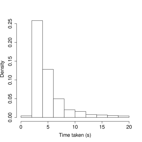
Figure 4: The distribution of the times taken for judges to make comparisons in the Nottinghamshire study.

6.1 Risk of Forced Marriage in Nottinghamshire

We fit the BSBT model using the Pólya-Gamma latent variable representation for 5,000 iterations, removing the first 50 iterations as a burn-in period. This took 54 seconds on a 2019 iMac with a 3 GHz CPU. We fixed the parameters for the inverse-Gamma prior distribution as $\chi=\omega=0.1$. Trace plots were examined to ensure the Markov chain had converged and mixed well, and are shown in the Supplementary Material.

The posterior median estimates for rate of forced marriage are shown in Figure 5. We see a divide between urban and rural areas in the county, with the ten wards with the highest rates all in the city of Nottingham. Mansfield is the other main urban centre in the county that is noticeable in the results. However, not all urban centres in the county are estimated to have a high rate of forced marriage with Worksop and Newark both ranked in the bottom third of wards. This suggests the judges were not making judgements based on population size. The posterior distribution for the covariance hyperparameter $\alpha$ is also shown in Figure 6; the posterior median is 14.8 with 95% credible interval (7.39, 40.8).

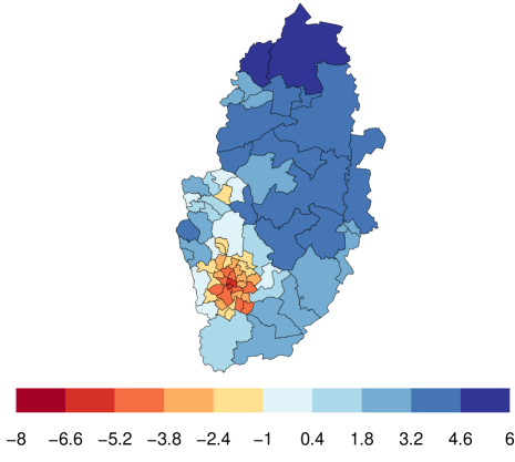
Figure 5: Left: A map of the wards in Nottinghamshire showing the results of the forced marriage study. The wards are coloured by the posterior median estimate for the rate for forced marriage. The wards with the highest rate are coloured in red, the lowest in blue. Right: The posterior distribution for the hyperparameter $\alpha$.

Figure 6 shows the posterior variance for each ward and the posterior variance compared against the posterior median. There is a clear relationship between the posterior median and variance of the rate parameters, where wards with very high or low rate have the largest posterior variance. This suggests some disagreement between these judges on the magnitude of these more extreme rate parameters.

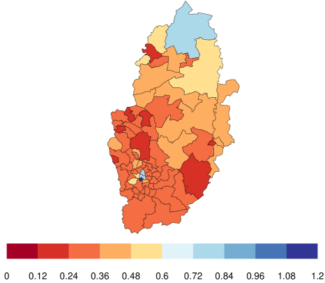
Figure 6: The uncertainty in the results for the Nottinghamshire forced marriage study. Left: The wards are coloured by the variance in the posterior distribution. Right: The posterior median estimate for rate of forced marriage against the variance of the posterior distribution.

6.2 Sensitivity Analysis for Judge Twelve

Judge 12 made over 1,000 comparisons over a period spanning one hour 40 minutes. This is a vastly higher number of comparisons than any other judge, representing around 60% of the total number of comparisons. We carried out a sensitivity analysis to assess the effect of this judge’s comparisons and as a form of quality assurance for our analysis. For the analysis, we fitted the model to three data sets: All. all the comparisons, Not 12. all the comparisons excluding judge 12, and Only 12. only the comparisons from judge 12.

We fitted the model to the three data sets in the same manner as to the full data set, running the MCMC algorithm for 5,000 iterations. Table 3 shows the Pearson and Spearman’s rank correlation coefficients between the estimates for the rate parameters $\boldsymbol{\lambda}$ for each pair of data sets. Both coefficients show a high level of agreement between judge 12 and the other judges. Removing the comparisons from judge 12 has little effect on the ordering of the wards (Spearman’s rank correlation coefficient 0.933). Maps and scatterplots of the relative rates showing that our conclusions are not sensitive to the data from judge 12 are provided in the Supplementary Material.

Data set	All	Not 12
Not 12	0.923	-
Only 12	0.971	0.832

Data set	All	Not 12
Not 12	0.933	-
Only 12	0.976	0.861

Table 3: The correlation coefficient (left) and Spearman’s rank correlation coefficient (right) between the estimates for the rate parameters $\lambda$.

6.3 Clustering for Forced Marriage in Nottinghamshire

To identify clusters of wards that have similar levels of forced marriage and are nearby, we fit the spatial clustering BT model described in Section 2.3. We describe the spatial relationship between the wards through the matrix exponential of the county’s adjacency matrix, i.e. $f(i,j)=(\exp A)_{i,j}$, which matches the prior distribution in the BSBT model. We ran the MCMC algorithm for 100,000 iterations, removing the first 1,000 iterations as burn-in period. We fix the concentration parameter $\beta=1\times 10^{-8}$ based on Ghosh et al., (2011). We ran a sensitivity analysis on the effect of different values of $\beta$, which is described in the Supplementary Material, and found this value had very little impact on the results. Each run of the MCMC algorithm took 45 minutes on a 2019 iMac with a 3 GHz CPU.

The model identifies three clusters of wards in the county and these are shown in Figure 7, alongside violin plots for the rate of forced marriage in the clusters and the posterior distribution for the number of clusters. There is little uncertainty about the number of clusters, with the model assigning a probability of 0.637 to there being three clusters, 0.188 to two clusters and 0.156 to four clusters. In the case of two clusters, clusters one and two (red and yellow in Figure 7) are merged, and in the case of four clusters the Nottingham urban area is split into inner and outer city clusters.

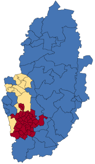
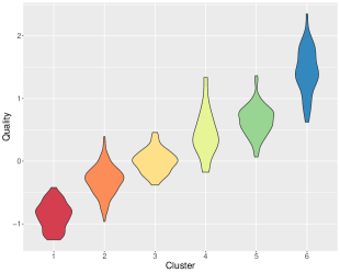
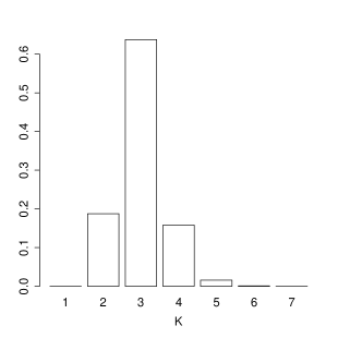
Figure 7: Left: A map of Nottinghamshire with the wards clustered by geolocation and rate of forced marriage. Middle: Violin plots showing the distribution of the rate in each cluster. Right: The posterior probabilities for the number of clusters in the county.

Focusing on the three cluster model, the clusters can be interpreted both as high-medium-low rate areas and through their geolocation. Cluster one consists of wards with high rates of forced marriage and broadly aligns with the Office for National Statistics definition of the Nottingham urban area. The second cluster consists of wards with middling rares of forced marriage and aligns with the Mansfield urban area and a nearby Nottingham suburb. The third cluster is the remainder of the county and forms a cluster of wards with low rates of forced marriage.

Figure 8 compares the results from the BSBT model to the clustering model. We find little substantive difference between the posterior medians. The clustering model shows some slight shrinkage in the posterior medians compared to the BSBT model. The clustering model however does show reduced uncertainty in the estimates, one reason for this may be because the concentration parameter $\beta$ in the clustering model is fixed, whereas the signal variance parameter $\alpha^{2}$ in the BSBT model is inferred. Overall, there are marginal differences in the estimates from both models and the clustering model provides results that are easier to interpret compared to the BSBT model.

Figure 8: Scatter plots comparing the posterior medians (left) and posterior variances (right) of the BSBT and spatial clustering model.

7 Discussion

Identifying high risk areas for forced marriage is an important step to prevent people from being forced into marriages. Current data on forced marriage in the UK is not avaliable at a local level, which limits the interventions that safeguarding professionals can design and implement. Comparative judgement studies are well suited to generate risk maps with high spatial resolution, but are limited to applications where are large number of people can be called upon as judges. By developing an efficient scheduling mechanism, we were able to collect comparative judgement data from a limited number of judges. This allowed us to generate ward level risk estimates for forced marriage in the county of Nottinghamshire, UK. Using Bayesian nonparametric methods, we were able to cluster the wards by both risk and geolocation, providing information on forced marriage to support the county’s Strategy on Tackling Violence Against Women and Girls.

We developed a policy briefing (see Supplementary Material) based on our findings and shared this widely with practitioners across the county. We also ran three in-person and online briefings with attendance from councillors, police officers, local authority support staff, housing agency workers and faith leaders. We showed how our findings can be used to inform safeguarding practices for forced marriage. Our risk maps identify wards in Nottinghamshire where front-line local authority workers should be alerted to the increased risk of forced marriage. Research has shown that schools and colleges can act as a support network for potential victims (Khan and Mikuska,, 2021) and schools and colleges in wards we identify as high risk can work with social services to support potential victims.

Our methods can also be used to improve forced marriage statistics nationally. We ran two in-person sessions with Members of the UK’s Parliament (MPs) and wrote to the Minister for Safeguarding to discuss these findings and improving national forced marriage statistics. MPs were then able to table questions in parliament asking the Government to improve its reporting on forced marriage statistics and making data available at ward level (see, e.g., HC Deb, 2022a, ; HC Deb, 2022b, ). Our research findings were also accepted as evidence to the House of Commons Committee of Public Accounts’ inquiry into protecting vulnerable adolescents (Seymour and McCabe,, 2022) and the Women and Equalities Committee’s inquiry into so-called honour based abuse (McCabe et al.,, 2022). In October 2022, the Minster for Safeguarding wrote to say “the research you have shared complements the wider work of the Government in this area” and the Government has “committed to explore options to better understand the prevalence of forced marriage”.

We collected over 1,800 comparisons from experts in forced marriage across the county. All comparisons were collected remotely via an online interface we developed. The interface worked successfully, however lacked a counter for the number of comparisons made, which led to one judge providing many more comparisons than others. Future studies should consider either limiting the number of comparisons a single judge can make or showing them a counter with the number of comparisons made so far and a recommended maximum number of comparisons. The minimum number of comparisons required to run a comparative judgement study is still an open question and methodological work on posterior contraction rates may provide clearer estimates for the amount of data that needs to be collected. Finally, further work could enable adaptive scheduling of comparisons, updating the prior distribution using the comparisons collected up to a given point.

Our study showed that comparative judgement can be used as a tool to map human rights abuses, such as forced marriage, at a high spatial resolution. This can provide local level information on human rights abuses and inform the design and implementation of safeguarding interventions. Bayesian computational methods are able to reduce the need for a large number of study participants and provide relevant results to local stakeholders.

SUPPLEMENTARY MATERIAL

Supplementary Material:

A simulation study of the MCMC algorithm and sensitivity analyses of the model. (.pdf file)

R Code to reproduce analysis:

All code used in the analysis and simulation studies. It also includes the shape files for Nottinghamshire and data collected. (Zipped file)

Policy briefing:

Non-technical briefing shared with MPs and councillors. (.pdf file)

Comparisons:

A 1,864 $\times$ 4 table containing the winner and loser of each comparison, the ID of the user who made the comparisons and the time it was made. (.csv file)

Results

A 76 $\times$ 5 table containing the name, posterior median, 5% and 95% quantiles and posterior variance of each ward (.csv file).

References

- Bates, (2020) Bates, L. (2020). Honor-based abuse in England and Wales: Who does what to whom? Violence Against Women, 27(10):1774–1795.
- Blei and Frazier, (2011) Blei, D. M. and Frazier, P. I. (2011). Distance dependent Chinese restaurant processes. Journal of Machine Learning Research, 12(74):2461–2488.
- Bradley and Terry, (1952) Bradley, R. A. and Terry, M. E. (1952). Rank analysis of incomplete block designs: I. the method of paired comparisons. Biometrika, 39(3/4):324–345.
- Caron and Doucet, (2012) Caron, F. and Doucet, A. (2012). Efficient Bayesian inference for generalized Bradley–Terry models. Journal of Computational and Graphical Statistics, 21(1):174–196.
- Cattelan et al., (2012) Cattelan, M., Varin, C., and Firth, D. (2012). Dynamic Bradley–Terry modelling of sports tournaments. Journal of the Royal Statistical Society: Series C, 62(1):135–150.
- Chantler et al., (2021) Chantler, K., Mirza, N., and Mackenzie, M. (2021). Policy and professional responses to forced marriage in Scotland. The British Journal of Social Work, 52(2):833–849.
- Devroye, (1986) Devroye, L. (1986). Non-Uniform Random Variate Generation. Springer New York.
- Estrada and Higham, (2010) Estrada, E. and Higham, D. J. (2010). Network properties revealed through matrix functions. SIAM Review, 52(4):696–714.
- Forced Marriage Unit, (2019) Forced Marriage Unit (2019). Forced marriage unit statistics 2019. Technical report, Foreign, Commonwealth & Development Office, and the Home Office.
- Ghosh et al., (2011) Ghosh, S., Ungureanu, A., Sudderth, E., and Blei, D. (2011). Spatial distance dependent Chinese restaurant processes for image segmentation. In Shawe-Taylor, J., Zemel, R., Bartlett, P., Pereira, F., and Weinberger, K., editors, Advances in Neural Information Processing Systems, volume 24. Curran Associates, Inc.
- Glickman and Jensen, (2005) Glickman, M. E. and Jensen, S. T. (2005). Adaptive paired comparison design. J. Stat. Plan. Inference, 127(1-2):279–293.
- Graßhoff and Schwabe, (2008) Graßhoff, U. and Schwabe, R. (2008). Optimal design for the Bradley–Terry paired comparison model. Statistical Methods and Applications, 17(3):275–289.
- Guo et al., (2018) Guo, Y., Tian, P., Kalpathy-Cramer, J., Ostmo, S., Campbell, J. P., Chiang, M. F., Erdogmus, D., Dy, J. G., and Ioannidis, S. (2018). Experimental design under the Bradley–Terry model. In Proceedings of the Twenty-Seventh International Joint Conference on Artificial Intelligence, pages 2198–2204.
- (14) HC Deb (2022a). 45683. https://questions-statements.parliament.uk/written-questions/detail/2022-09-02/45683.
- (15) HC Deb (2022b). 61026. https://questions-statements.parliament.uk/written-questions/detail/2022-10-11/61026.
- Home Affairs Commmittee, (2008) Home Affairs Commmittee (2008). Domestic Violence, Forced Marriage and “Honour”- Based Violence: Further Government Response to the Committee’s Sixth Report of Session 2007–08. Technical report.
- Khan and Mikuska, (2021) Khan, T. and Mikuska, É. (2021). The first three weeks of lockdown in England: The challenges of detecting safeguarding issues amid nursery and primary school closures due to COVID-19. Social Sciences and Humanities Open, 3(1):100099.
- Mardia et al., (1979) Mardia, K. V., Kent, J. T., and Bibby, J. M. (1979). Multivariate Analysis. Probability and Mathematical Statistics. Academic Press, San Diego, CA.
- Marshall, (2020) Marshall, H. (2020). Understanding demand for songbirds within Indonesia’s captive bird trade. PhD thesis, Manchester Metropolitan University, Manchester.
- McCabe et al., (2022) McCabe, H. R., Seymour, R. G., Schwarz, K., Eglen, L., and Brown, R. (2022). Written evidence HBA0016. Technical report, Women and Equalities Select Committee.
- Office of the Police and Crime Commissioner in Nottinghamshire, (2021) Office of the Police and Crime Commissioner in Nottinghamshire (2021). Violence against Women and Girls Strategy, Nottingham and Nottinghamshire 2021-2025. Technical report.
- Polson et al., (2013) Polson, N. G., Scott, J. G., and Windle, J. (2013). Bayesian inference for logistic models using Pólya–Gamma latent variables. Journal of the American Statistical Association, 108(504):1339–1349.
- Ryan et al., (2015) Ryan, E. G., Drovandi, C. C., McGree, J. M., and Pettitt, A. N. (2015). A review of modern computational algorithms for Bayesian optimal design. International Statistical Review, 84(1):128–154.
- Seymour and McCabe, (2022) Seymour, R. G. and McCabe, H. R. (2022). Written evidence SVA0006. Technical report, Committee of Public Accounts.
- Seymour et al., (2022) Seymour, R. G., Sirl, D., Preston, S. P., Dryden, I. L., Ellis, M. J. A., Perrat, B., and Goulding, J. (2022). The Bayesian Spatial Bradley–Terry Model: Urban Deprivation Modelling in Tanzania. Journal of the Royal Statistical Society Series C, 71(2):288–308.
- Turner and Firth, (2012) Turner, H. and Firth, D. (2012). Bradley-Terry models in R: The BradleyTerry2 package. Journal of Statistical Software, 48(9).