Denoising after Entropy-based Debiasing
A Robust Training Method for Dataset Bias with Noisy Labels

Abstract

Improperly constructed datasets can result in inaccurate inferences. For instance, models trained on biased datasets perform poorly in terms of generalization (i.e., dataset bias). Recent debiasing techniques have successfully achieved generalization performance by underestimating easy-to-learn samples (i.e., bias-aligned samples) and highlighting difficult-to-learn samples (i.e., bias-conflicting samples). However, these techniques may fail owing to noisy labels, because the trained model recognizes noisy labels as difficult-to-learn and thus highlights them. In this study, we find that earlier approaches that used the provided labels to quantify difficulty could be affected by the small proportion of noisy labels. Furthermore, we find that running denoising algorithms before debiasing is ineffective because denoising algorithms reduce the impact of difficult-to-learn samples, including valuable bias-conflicting samples. Therefore, we propose an approach called denoising after entropy-based debiasing, i.e., DENEB, which has three main stages. (1) The prejudice model is trained by emphasizing (bias-aligned, clean) samples, which are selected using a Gaussian Mixture Model. (2) Using the per-sample entropy from the output of the prejudice model, the sampling probability of each sample that is proportional to the entropy is computed. (3) The final model is trained using existing denoising algorithms with the mini-batches constructed by following the computed sampling probability. Compared to existing debiasing and denoising algorithms, our method achieves better debiasing performance on multiple benchmarks.

1 Introduction

Deep neural networks (DNNs) have achieved human-like performance in various tasks, such as image classification (He et al. 2016), image generation (Goodfellow et al. 2014), and object detection (He et al. 2017), but require well-organized training datasets for success. For example, the trained model might have prejudices when its training dataset is biased. In real life, we often encounter dataset bias problems (Bahng et al. 2020; Nam et al. 2020; Lee et al. 2021; Kim, Lee, and Choo 2021). For example, as shown in Figure 1, the dataset for classifying camels in images could be very biased, as most camel images are captured against a desert background (i.e., bias-aligned); only a few images are captured against other backgrounds, such as forests (i.e., bias-conflicting). This unintended bias causes the trained model to infer erroneously based on shortcuts (i.e., background). To mitigate such dataset bias, previous researches have used the fact that bias-conflicting samples are more difficult-to-learn than bias-aligned samples (Nam et al. 2020). Various approaches have been proposed, such as adjusting the loss function (Bahng et al. 2020; Nam et al. 2020; Creager, Jacobsen, and Zemel 2021), feature disentanglement (Lee et al. 2021), creating mixed-attribute samples (Kim, Lee, and Choo 2021), or reconstructing balanced datasets (Liu et al. 2021; Ahn and Yun 2021) to emphasize difficult-to-learn samples.

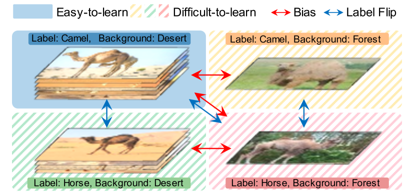
Figure 1: Examples of biased dataset with noisy labels. (1) Blue: bias-aligned, clean label samples. (2) Orange: bias-conflicting, clean labels samples. (3) Green: bias-aligned, noisy labels. (4) Red: bias-conflicting, noisy labels. The dashed background represents difficult-to-learn samples. Therefore, except for (bias-aligned, clean) case, other cases are difficult-to-learn. To mitigate dataset bias with noisy labels, training directions for each type differ. For example, (bias-aligned, noisy) case must be discarded or cleansed, while (bias-conflicting, clean) cases have to be emphasized.

In addition to dataset bias, noisy labels are caused by many reasons (Yu et al. 2018; Nicholson, Sheng, and Zhang 2016) and are known to degrade training mechanisms. For example, in Figure 1, the camel in the bottom row can be labeled horse by human error. Numerous studies have focused on alleviating the impact of noisy labels or directly correcting them. Some (Bahri, Jiang, and Gupta 2020; Zhang et al. 2020; Veit et al. 2017; Ren et al. 2018; Hendrycks et al. 2018) deal with the problem of noisy labels by assuming clean data to set training guidelines (i.e., purifying a given corrupted dataset by using a model trained on a small clean dataset). Recently, various methods have been proposed to relax this strong clean subset assumption by taking advantage of the characteristic that noisy labels are more difficult-to-learn than clean samples. For example, such difficult-to-learn samples are guided by regularizers (Liu et al. 2020; Cao et al. 2019, 2020), giving lower weights (Wang et al. 2019; Zhang and Sabuncu 2018), cleansing out (Mirzasoleiman, Cao, and Leskovec 2020; Wu et al. 2020; Pleiss et al. 2020; Han et al. 2018; Yu et al. 2019), or utilizing a semi-supervised learning algorithm by considering them as unlabeled samples (Kim et al. 2021; Li, Socher, and Hoi 2019).

Although dataset bias and noisy labels can occur simultaneously and independently, few studies (Creager, Jacobsen, and Zemel 2021) have addressed both problems at once. This is because the fundamental solutions of each problem are exact opposites. Difficult-to-learn samples have to be emphasized to mitigate dataset bias (Nam et al. 2020; Lee et al. 2021), while their influence should be reduced for denoising (Han et al. 2018; Zhang and Sabuncu 2018). Dataset bias and noisy labels can occur concurrently in the real-world. Therefore, both problems must be handled together.

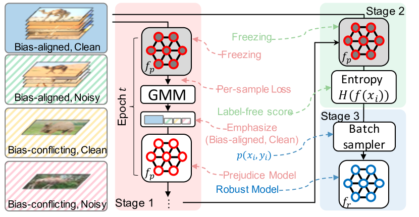
Figure 2: Overview of DENEB. It is composed of three steps. (1) Train by emphasizing (bias-aligned, clean) samples. (2) Compute label-free score, i.e., entropy. (3) Train the final robust model based on the batch sampler.

Contribution.  We present a training method that addresses dataset bias with noisy labels (DBwNL). We first empirically analyze why existing debiasing and denoising algorithms fail to achieve their respective objectives. In this regard, we discover two facts. (1) Existing debiasing methods using given labels suffer from problems when the training dataset contains noisy labels because they determine the degree of being emphasized based on a given label (e.g., per-sample loss). (2) Denoising methods eliminate valuable bias-conflicting samples (i.e., samples that should be emphasized for debiasing). This is because their denoising mechanism cleans or discards difficult-to-learn samples without considering whether a sample is bias-conflicting or noisy label.

Based on these findings, we propose an algorithm, coined as DENEB, which denoising after entropy-based debiasing (see Figure 2). The proposed method consists of three stages. The first stage trains a prejudice model biased toward (bias-aligned, clean) data. To this aim, DENEB  uses the Gaussian Mixture Model (GMM) based on per-sample losses to split (bias-aligned, clean) and the others at the beginning of each epoch. In the next stage, DENEB  measures the entropy for each sample from the prejudice model. From the per-sample entropy, DENEB  calculates the sampling probability of each sample in proportion to the entropy. The key intuition of the sampling probability is that (bias-aligned, noisy) samples are predicted to have low entropy by the prejudice model because it mainly learns (bias-aligned, clean) samples, but the excluded bias-conflicting samples will have a large entropy prediction. Note that the sampling probability is obtained without using the given labels as they might be corrupted. Finally, DENEB  trains the ultimate robust model on the sampled mini-batches, where the sampling probabilities are obtained during Step 2.

We demonstrate the efficacy of DENEB on a variety of biased datasets, including Colored MNIST (Nam et al. 2020; Bahng et al. 2020; Kim, Lee, and Choo 2021; Lee et al. 2021), Corrupted CIFAR-10 (Nam et al. 2020; Lee et al. 2021), Biased Action Recognition (BAR) (Nam et al. 2020; Kim, Lee, and Choo 2021), and Biased Flickr-Faces-HQ (Lee et al. 2021; Kim, Lee, and Choo 2021), with symmetric noisy labels. Compared to the existing debiasing, denoising, and naive combination of both algorithms, the proposed method achieves a successful debiasing performance for all benchmarks. For example, DENEB  improves the unbiased test accuracy from $39.24\%$ to $91.81\%$ on a colored MNIST dataset with $1\%$ bias scenario with $10\%$ noisy labels and BAR from $54.37\%$ to $62.30\%$ compared to the vanilla model.

2 Dataset Bias with Noisy Labels (DBwNL)

In this section, we define the dataset bias problem and the noisy label separately. Subsequently, we describe dataset bias with noisy labels, which is when dataset bias and noisy label problems occur in conjunction.

Dataset Bias.  Consider a dataset $\mathcal{D}=\{(x_{i},y_{i})\}_{i=1}^{N}$ in which each input is $x_{i}$ and its corresponding truth label $y_{i}=\{1,...,C\}$. Each sample can be described by a set of attributes. For example, the images in Figure 1 can have background, object, and so on. For convenience of explanation, we look at the top of Figure 1 (Blue and Orange cases), without the noisy label case. The objective, i.e., the target attribute, is to classify the “camel.” When most of the samples have attributes that are strongly correlated with the target, we call the phenomenon dataset bias and these attributes bias attributes. In Figure 1, the bias-attribute “desert background,” and the target attribute “camel” are highly correlated, i.e., almost “camel” images are captured against “desert background.” We call samples whose bias attribute is highly correlated (weakly correlated) with the target attribute bias-aligned (bias-conflicting) samples. This dataset bias problem is quite harmful when the bias attribute is easier to learn than the target attributes, because the model loses the motivation to learn the target attribute given its sufficiently low loss. We focus on the case where the bias attribute is easier to learn than the target. For convenience, we denote the set of bias-conflicting and bias-aligned samples by $\mathcal{D}_{c}$ and $\mathcal{D}_{a}$ as they are clearly distinct, but both sets need not be strictly separable. Note that the portion of bias-conflicting sample is called the bias conflict ratio $\alpha$, which is defined as:

$$\alpha=\frac{|\mathcal{D}_{c}|}{|\mathcal{D}|}.$$

Noisy Labels.  Collected labels may be corrupted. If a person labels the image $x$, the provided label can be corrupted i.e., $y_{\text{given}}\neq y$, even though the true label is $y$. We call samples whose labels are $y_{\text{given}}=y$ and $y_{\text{give}}\neq y$ clean label and noisy label, respectively. As shown in Figure 1, the lower row represents noisy label cases. For example, although the images in Figure 1 of the bottom boxes are “camel”, they are labeled as “horse”. We denote the portion of the samples whose labels are flipped as the noise ratio $\eta$. For convenience, we focus on the cases where the label corruption occurs symmetrically.

$$y_{\text{given}}=\begin{cases}\tilde{y}\sim\text{Uniform}(C).&\text{with probability }\eta\\ y&\text{with probability }1-\eta\end{cases},$$

DBwNL.  DBwNL cases occur sequentially, gathering images $x$ and labeling $y$. As mentioned above, the biased dataset has a small portion of bias-conflicting samples, i.e., $\alpha$ is small. Therefore, most of the samples in the given training dataset are bias-aligned. Training a robust model on the DBwNL dataset emphasizes bias-conflicting samples while discarding or reducing the impact of the noisy labels.

3 Failure to debias on a DBwNL dataset

In this section, we briefly summarize existing debiasing methods and demonstrate that they are vulnerable to noisy labels.

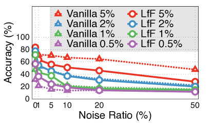
(a) LfF (Nam et al. 2020)

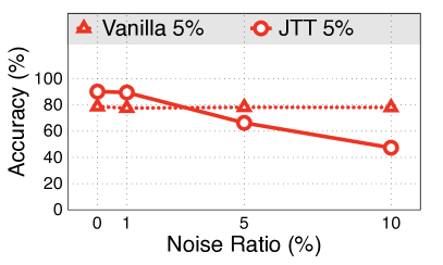
(b) JTT (Liu et al. 2021)

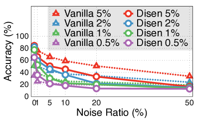
(c) Disen (Lee et al. 2021)

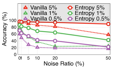
(d) Entropy

Figure 3: Performance when label corruption occurs. In the case of LfF and Disen, it is the unbiased test accuracy of colored MNIST, and JTT is the worst case test performance of the waterbird dataset. The triangle-dotted lines are the vanilla results, and the circle-solid lines represent the result of each algorithm. All algorithms except for entropy case perform worse than vanilla as noise ratio $\eta$ increases.

Brief summary of the previous methods.  In previous debiasing algorithms, bias-conflicting samples are highlighted based on each proposed score. Almost all previous approaches train a biased model $f_{b}$ on the given training dataset, and a debiased model $f_{d}$ is trained with emphasis in the following ways:

• Relative difficulty score (LfF (Nam et al. 2020), Disen (Lee et al. 2021))

  $$\mathcal{W}(x,\underline{\bm{y_{\text{given}}}})=\frac{\mathcal{L}_{\text{CE}}(f_{b}(x),\underline{\bm{y_{\text{given}}}})}{\mathcal{L}_{\text{CE}}(f_{b}(x),\underline{\bm{y_{\text{given}}}})+\mathcal{L}_{\text{CE}}(f_{d}(x),\underline{\bm{y_{\text{given}}}})},$$ (1)

  where $\mathcal{L}_{\text{CE}}$ denotes conventional cross-entropy loss and $f_{b}(\cdot)$ and $f_{d}(\cdot)$ are softmax outputs of biased and debiased models, respectively.

• Per-sample accuracy (JTT (Liu et al. 2021))

  $$\mathcal{D}_{\text{error-set}}=\{(x,y)\text{ s.t. }\underline{\bm{y_{\text{given}}}}\neq\operatorname*{arg\,max}_{c}f_{b}(x)[c]\},$$ (2)

  where $f_{b}(x)[c]$ denotes the softmax output of logit $c$. The ultimate debiased model is trained on $\mathcal{D}_{\text{train}}$ composed of $\lambda_{\text{up}}$ times $\mathcal{D}_{\text{error-set}}$ and the other $\mathcal{D}_{\text{corr-set}}=\mathcal{D}\setminus\mathcal{D}_{\text{error-set}}$.

3.1 Debiasing meets noisy labels

As in (1) and (2), all previous techniques are based on the given label $y_{\text{given}}$. Here, we refer to methods using $(x,y_{\text{given}})$ and only $(x)$ respectively as “label-based debiasing” and “label-free debiasing.” We observe the ultimate performance of previous methods when noisy labels are injected. We used the settings offered by their official repositories, such as dataset, implementation, and hyperparameters except for label flipping. For comparison, we include entropy-based debiasing, which highlights samples with proportion to the per-sample entropy score. It does not require the given label, i.e., label-free method. Detail description about entropy-based setting is described in Appendix.

Label-based debiasing is prone to noisy labels.  As shown in Figure 3, the performances of the label-based techniques are lower than those of the vanilla case; a small noise ratio occurs. However, as demonstrated in Figure 3d, the label-free method performs better than in the vanilla case. This is because label-based methods make incorrect emphasis, $\mathcal{W}(x,y_{\text{given}})$ and $\mathcal{D}_{\text{error-set}}$, when $y_{\text{given}}$ is corrupted.

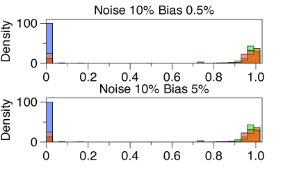
(a) LfF (Nam et al. 2020)

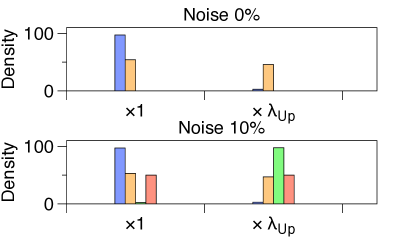
(b) JTT (Liu et al. 2021)

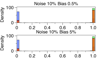
(c) Disen (Lee et al. 2021)

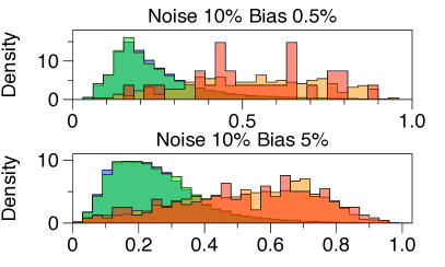
(d) Entropy

Figure 4: Score histogram of each methodology. As LfF and Disen operate online, we report the weight histogram right after the last epoch of training. Except for the Entropy case, LfF, JTT, and Disen shows entangled histograms between (noisy, aligned), (clean, conflicting), and (noisy, conflicting). By contrast, the histogram of entropy case indicates that it is clustered not according to label corruption but bias.

Why do label-based methods suffer side-effects?  As in Figure 5a 5b, and 5c, the label-based scores of the (conflicting, clean) and (aligned, noisy) are entangled. This means that noisy labels are also emphasized when we run the labe-based algorithms. By contrast, the label-free method, i.e., Entropy in Figure 5d, shows that the bias-conflicting and bias-aligned samples are easily distinguished regardless of whether their labels are noisy. In conclusion, a label-free method is needed to handle DBwNL.

4 DENoising after Entropy-based DeBiasing

In Section 3, we verified that the debiasing algorithms do not work properly for DBwNL alone. In this section, we analyze how debiasing algorithms should be combined with denoising algorithms, and finally propose DENEB.

4.1 How denoising algorithms work in the DBwNL

We first check how the denoising algorithms work in the DBwNL dataset by observing two cases.

Observation Setting.  Five denoising methods are used for the analysis: AUM (Pleiss et al. 2020), Co-teaching (Han et al. 2018), DivideMix (Li, Socher, and Hoi 2019), and f-DivideMix (Kim et al. 2021). We measure the number of samples of (noisy, aligned) and (clean, conflicting) after running the denoising algorithms. We run two types of tests. (1) Without modification (✗): to check how the denoising algorithms handle bias-conflicting samples. (2) Manually weighted training ($\CIRCLE$): we assign $\times 50$ weights to bias-conflicting samples, i.e., $50\times\mathcal{L}_{\text{CE}}(x,y)$, $\forall(x,y)\in\mathcal{D}_{c}$. The second case is unrealistic as we cannot know which sample is bias-conflicting, but the result can convey the following argument: if we want to protect bias-conflicting samples from the discarding by the denoising mechanism, make the bias-conflicting samples easy-to-learn.

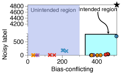
(a) $\alpha=1\%$, $\eta=10\%$

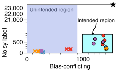
(b) $\alpha=5\%$, $\eta=50\%$

Figure 5: Number of remaining noisy labels and bias-conflicting samples after denoising is conducted. Star $\star$ mark represents the number of samples before cleansing, and ✗  and $\CIRCLE$ marks indicate with or without weighted training results. Since bias-conflicting samples is precious for debiasing, bias-conflicting samples have to be protected. Therefore, the region loses bias-conflicting samples (left, blue) is the unintended region. On the other hand, the region ignores noisy labels without losing the bias-conflicting samples (right, cyan) is the intended behavior.

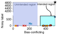
(a) $\alpha=1\%$, $\eta=10\%$

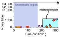
(b) $\alpha=1\%$, $\eta=50\%$

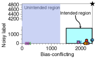
(c) $\alpha=5\%$, $\eta=10\%$

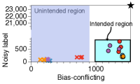
(d) $\alpha=5\%$, $\eta=50\%$

Figure 6: Number of remaining noisy labels and bias-conflicting samples after denoising is conducted. Star $\star$ mark represents the number of samples before cleansing, and ✗  and $\CIRCLE$ marks indicate with or without weighted training results. Since bias-conflicting samples is precious for debiasing, bias-conflicting samples have to be protected. Therefore, the region loses bias-conflicting samples (left, blue) is the unintended region. On the other hand, the region ignores noisy labels without losing the bias-conflicting samples (right, cyan) is the intended behavior.

Valuable bias-conflicting samples can be deemed noisy.  As illustrated in Figure 5, all denoising methods sufficiently differentiate noisy samples. For example, $\star$ in Figure 6a represents that the initial number of noisy samples is almost $5,000$, but almost all methods dropped to near $0$ after denoising (✗  marks). However, crucial bias-conflicting samples are also eliminated, i.e., ✗  marks are in the “unintended region.” Therefore, utilizing denoising algorithms before debiasing can discard valuable bias-conflicting samples. As in Figure 3, because the number of bias-conflicting samples is critical, removing the bias-conflicting samples prior to debiasing can cause performance degradation.

Preventing bias-conflicting samples from being discarded.  Bias-conflicting samples are considered noisy labels because the trained model thinks that they are difficult-to-learn. As illustrated in Figure 5 using $\CIRCLE$ marks, when we sufficiently highlight bias-conflicting samples, noisy labels can be eliminated by reducing the loss of bias-conflicting samples. Therefore, we can conclude that denoising should be performed after highlighting bias-conflicting samples.

4.2 Designing the Algorithm for DBwNL

Based on the previous experimental results, two inferences can be drawn in designing a debiasing algorithm for the DBwNL datasets. (1) No label-based: label-based debiasing emphasizes noisy labels. (2) Debiasing before denoising: denoising algorithms should be run after debiasing emphasizes bias-conflicting samples. We summarize our intuitions in Figure 6. For the DBwNL dataset, the main consideration is whether to apply debiasing or denoising first. If denoising is applied first, the bias-conflicting samples is erased, which is burdensome for debiasing (see the lower $\alpha$ cases in Figure 3). Conversely, if debiasing is conducted first, we can choose label-based or label-free. If a label-based algorithm is selected, the noisy labels are enlarged and a burden is placed on the denoising algorithm (see the higher $\eta$ cases in Figure 3). In other words, emphasizing the bias-conflicting sample and proceeding with denoising without emphasizing the noisy label through the label-free algorithm is the correct order.

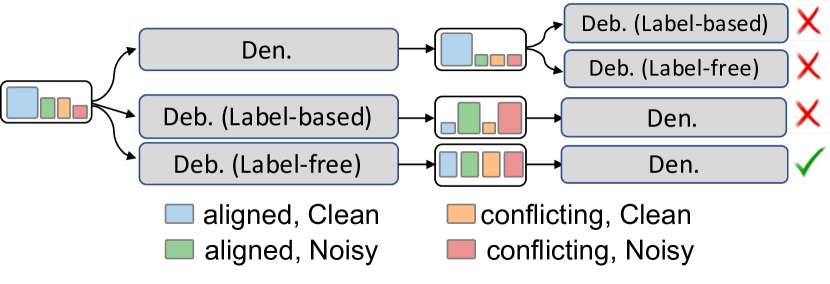
Figure 6: Case study of designing algorithm for DBwNL.

4.3 Denoising after entropy-based Debiasing

Based on the case study, we propose denoising after entropy-based debiasing, DENEB, which is composed of three steps.

Step 1: Train the prejudice model $f_{p}$.  The key aim while training the prejudice model $f_{p}$ is that regardless of label corruption, the model should comprehensively learn the bias-aligned samples so that it can identify the bias-conflicting samples in the next steps. However, it is difficult to detach (bias-aligned, noisy) from the bias-conflicting samples. Therefore, DENEB  trains the prejudice model on (bias-aligned, clean) only. Intuitively speaking, if the model is trained using only (bias-aligned,clean) samples, (bias-aligned,noisy) samples also can be regarded as easy-to-learn thanks to the bias attributes. DENEB  finds (bias-aligned, clean) by using the GMM, similar with (Li, Socher, and Hoi 2019; Kim et al. 2021). Step 1 consists of two sub-steps. At first, $f_{p}$ is trained on $\mathcal{D}$ with conventional cross-entropy loss, until the warm-up epoch $e_{w}$. After the warm-up phase, DENEB  splits $\mathcal{D}$ and obtains $\bar{\mathcal{D}}$ at the beginning of each epoch. To do so, DENEB  dynamically fits a GMM on per-sample losses and obtains $\bar{\mathcal{D}}$ whose probability of GMM $g(x_{i},y_{i})$ is higher than the threshold $p_{t}$ at the beginning of each epoch:

$$\bar{\mathcal{D}}=\{(x_{i},y_{i})|g(x_{i},y_{i})>p_{t},\text{ where }(x_{i},y_{i})\in\mathcal{D}\},$$ (3)

Note that, unlike DivideMix and f-DivideMix, DENEB does not use the samples whose $g(x_{i},y_{i})\leq p_{t}$, to deepen bias, i.e., it ignores every-types except for (bias-aligned,clean).

Step 2: Calculate sampling probability.  Based on the trained prejudice model $f_{p}$, we extract the entropy score for each sample:

$$H_{\tau}(x)=-\sum_{c}^{C}f_{p}(x,\tau)[c]\times\log f_{p}(x,\tau)[c],$$ (4)

where $f_{p}(x,\tau)[j]$ is the temperature-scaled softmax for class $c$ with temperature parameter $\tau$, i.e., $f_{p}(x,\tau)[j]=\frac{\exp(q_{p}(x)[j]/\tau)}{\sum_{c}\exp(q_{p}(x)[c]/\tau)}$ with logit $q_{p}(x)$. Based on $H_{\tau}(x)$, we find the sampling probability of each instance as follows:

$$\mathcal{P}(x_{i},y_{i})=\frac{H_{\tau}(x_{i})}{\sum_{(x_{j},y_{j})\in\mathcal{D}}H_{\tau}(x_{j})}.$$ (5)

The reason why $\mathcal{P}(x_{i},y_{i})$ is proportional to the entropy score is because $f_{p}$ is sufficiently biased and thus the larger entropy samples are the bias-conflicting samples (see Figure 5d).

Step 3: Train the robust model $f_{r}$.  To train the robust model $f_{r}$, mini-batches are constructed based on the sampling probability in equation 5. As mini-batches contain sufficient bias-conflicting samples, the main purpose of this step is to mitigate the impact of noisy labels. To this end, we inherit previous denoising algorithms by simply modifying the mini-batches. Note that DENEB  can utilize any given denoising algorithm, $\mathcal{A}_{\text{den}}$, but we report based on GCE which performs better than the others. As analysis of various denoising algorithms is reported in Section 5.

5 Experiment

The effectiveness of the proposed algorithm is analyzed quantitatively and qualitatively. We compare DENEB to earlier debiasing and denoising techniques in four biased datasets, i.e., Colored-MNIST (CMNIST), Corrupted CIFAR-10 (CCIFAR), Biased Action Recognition (BAR), and Biased FFHQ (BFFHQ). To test the generalization performance, we report the unbiased test accuracy. Details of the implementation and datasets are given in Appendix.

Table 1: Benchmark Summary

4Dataset	train/valid/test	#class	Target	Bias
CMNIST	54K / 6K / 10K	10	Shape	Color
CCIFAR	45K / 5K / 10K	10	Object	Blur
BAR	1,746 / 195 / 654	6	Action	Place
BFFHQ	17,280/1,920/1,000	2	Gender	Age
4

Table 2: Unbiased test accuracy on CMNIST and CCIFAR. Best-performing results are marked in bold. All results are averaged on three independent runs. DENEB represents i.e., $\mathcal{A}_{\text{den}}=$ GCE.

4Algorithm	Colored MNIST		Corrupted CIFAR-10
	$\alpha=1$%, $\eta=10\%$	$\alpha=5$%, $\eta=50\%$	$\alpha=1$%, $\eta=10\%$	$\alpha=5$%, $\eta=50\%$
Vanilla	39.24 $\pm$ 1.91%	70.13% $\pm$ 3.42 %	25.43% $\pm$ 0.84 %	31.86% $\pm$ 0.96 %
Debiasing
LfF	29.87 $\pm$ 1.36%	57.97% $\pm$ 1.79 %	24.51% $\pm$ 1.30 %	29.68% $\pm$ 2.63 %
JTT	63.24 $\pm$ 2.60%	77.16% $\pm$ 1.15 %	23.75% $\pm$ 0.61 %	24.52% $\pm$ 0.98 %
EIIL	24.53 $\pm$ 0.31%	42.25% $\pm$ 1.43 %	20.30% $\pm$ 1.08 %	22.66% $\pm$ 1.94 %
Disen	31.49 $\pm$ 5.44%	69.20% $\pm$ 4.13 %	22.52% $\pm$ 0.38 %	28.35% $\pm$ 4.49 %
Denoising
GCE	19.52 $\pm$ 1.98%	73.45% $\pm$ 7.62 %	24.96% $\pm$ 1.53 %	30.72% $\pm$ 0.74 %
SCE	30.95 $\pm$ 2.87%	62.10% $\pm$ 5.02 %	23.34% $\pm$ 1.73 %	29.87% $\pm$ 1.00 %
ELR+	24.76 $\pm$ 0.90%	49.38% $\pm$ 3.74 %	22.10% $\pm$ 0.37 %	30.84% $\pm$ 0.43 %
AUM	23.89 $\pm$ 2.60%	49.51% $\pm$ 6.62 %	23.55% $\pm$ 1.10 %	28.06% $\pm$ 2.38 %
Co-teaching	41.89 $\pm$ 1.45%	76.64% $\pm$ 5.52 %	25.14% $\pm$ 0.27 %	26.84% $\pm$ 0.52 %
DivideMix	20.48 $\pm$ 1.94%	33.66% $\pm$ 2.91 %	18.86% $\pm$ 0.28 %	22.03% $\pm$ 0.59 %
f-DivideMix	22.06 $\pm$ 1.70%	39.92% $\pm$ 3.26 %	19.67% $\pm$ 0.25 %	27.60% $\pm$ 0.54 %
DENEB
DENEB	91.81 $\pm$ 0.84%	94.55% $\pm$ 0.22 %	26.05% $\pm$ 0.54 %	35.32% $\pm$ 1.03 %
4

Table 3: Unbiased test accuracy on BAR and BFFHQ. Best performing results are marked in bold. All results are averaged on three independent runs.

4Algorithm	BAR	BFFHQ
	$\eta=10\%$	$\eta=10\%$
Vanilla	54.37 $\pm$ 1.10%	71.38 $\pm$ 0.58%
LfF	53.62 $\pm$ 1.81%	54.35 $\pm$ 0.91%
JTT	55.67 $\pm$ 2.16%	70.18 $\pm$ 1.47%
Disen	55.80 $\pm$ 3.05%	67.44 $\pm$ 2.57%
GCE	56.39 $\pm$ 0.95%	68.45 $\pm$ 2.98%
Co-teaching	54.99 $\pm$ 1.28%	69.28 $\pm$ 1.24%
DivideMix	52.01 $\pm$ 1.51%	72.20 $\pm$ 0.58%
DENEB	62.30 $\pm$ 0.91%	75.24 $\pm$ 0.68%
4

5.1 Experimental settings

Baselines.  We report the performance of the debiasing and denoising algorithms. As debiasing algorithms, we use recent methods that are officially available, such as LfF, JTT, EIIL, and Disen. We utilize denoising algorithms GCE, SCE, ELR+, Co-teaching, DivideMix, and f-DivideMix. All implementations are reproduced following the official codes. The implementation and hyperparameters are reported in Appendix.

Datasets.  We employ four benchmarks: CMNIST, CCIFAR, BAR, and BFFHQ. The target and bias attributes are summarized in Table 1. For the CMNIST and CCIFAR datasets, two pairs of bias-ratio $(\alpha,\eta)=\{(1\%,10\%),(5\%,50\%)\}$ are utilized. The other datasets are tested on $\eta=10\%$. We summarize in detail the construction recipe in Appendix.

CMNIST and CCIFAR.  CMNIST and CCIFAR datasets have a bias attribute, which is injected manually. The goal of CMNIST is to classify the target attribute, digit shape, when the bias attribute is color. This dataset comes from (Nam et al. 2020; Bahng et al. 2020; Lee et al. 2021; Kim, Lee, and Choo 2021). In CCIFAR, the target attribute is objective such as {airplane, car,…} with the bias attribute corruption like {blur, gaussian noise, …}. We generate CCIFAR following the bias injection mechanism of (Nam et al. 2020; Lee et al. 2021; Hendrycks and Dietterich 2018).

BAR and BFFHQ.  BAR and BFFHQ are consists of real-world images. These benchmarks are biased when selecting samples by seeing the multiple attributes. BAR (Nam et al. 2020) aims to classify actions such as {racing, climbing,…} with background bias. For example, (Climbing, Rockwall) are bias-aligned samples, while (Climbing, Ice-cliff) are the bias-conflicting ones. BFFHQ (Kim, Lee, and Choo 2021; Lee et al. 2021) aims to classify gender when its age is biased. For example, the training dataset is made up of (Female, Young (age ranging from 10 to 29)) and (Male, Old (age ranging from 40 to 59)) and very few of (Female, Old) and (Male, Young) samples.

Implementation details.  For the Colored MNIST, we use a Simple-ConvNet with three convolutional layers, ReLU activation function (Agarap 2018), batch normalization (Ioffe and Szegedy 2015) and dropout (Srivastava et al. 2014). ResNet-18 (He et al. 2016) pre-trained on ImageNet is used as a backbone network for the rest. Based on grid searches, we find hyperparameters for all algorithms using $90\%$ and $10\%$ training and validation split. This implies that validation datasets contain noisy labels and bias-conflicting samples. The search space and searched hyperparameters are described in Appendix. For all experiments, we report the case where DENEB  uses GCE as $\mathcal{A}_{\text{den}}$, which achieves the best performance among all the denoising algorithms.

5.2 Experimental results

CMNIST and CCIFAR.  Table 2 presents comparisons of the accuracy of the unbiased test. Among the debiasing baselines, the accuracy-based algorithm, i.e., JTT, is better than the vanilla model in the CMNIST case. However, all debiasing baselines obtain worse performance than the vanilla model in the CCIFAR case because, as mentioned earlier, the debiasing algorithms highlight noisy labels that should not be emphasized. By contrast, denoising algorithms fail to debias, as they do not have a module to highlight bias-conflicting samples. DENEB  achieves the best performance for all injected bias cases. For example, the unbiased test accuracy of CMNIST with $\alpha=1\%$ and $\eta=10\%$ shows that DENEB  obtains $52.57\%$ gain compared to the Vanilla model.

BAR and BFFHQ.  The performances of DENEB  in real-world image benchmarks is also better than the other baselines. BAR shows $7.92\%$ improvements over vanilla and $6.5\%$ improvement over Disen, which has the best performance among the debiasing algorithms. DENEB  also shows $5.91\%$ performance gain over GCE. Similarly, BFFHQ shows $3.86\%$ improvement over vanilla, $5.06\%$ over JTT and $3.04\%$ over DivideMix. Thus, entropy-based debiases when trained on a more complex raw image dataset.

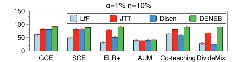
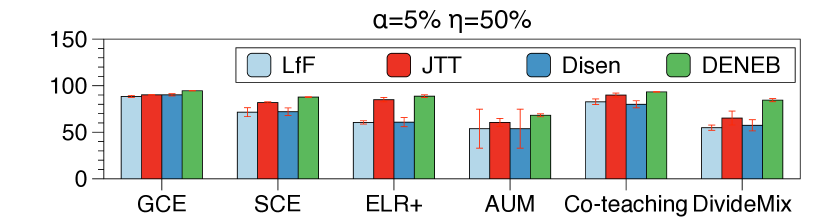
Figure 7: Combination result of Colored MNIST benchmark. All cases are the performances of Debiasing $\to$ Denoising, i.e., obtain per-sample weights from DENEBand then run GCE for DENEB$\to$GCE case.

Combination of Debiasing and Denoising.  In order to study how the other debiasing algorithms work with denoising algorithms, i.e., debiasing $\to$ denoising similarly to DENEB, we report pairwise performance in Figure 7 for CMNIST. As Disen and LfF are an online algorithms, we multiply the per-sample weight at the end of debiasing by denoising loss. Details are provided in Appendix. As shown in Figure 7, DENEB  performs better than the other debiasing algorithms for all combinations. DENEB  has better performance because the side-effects of focusing on the noisy sample are minimized when using the label-free entropy.

6 Related work

Noisy labels.  (Ghosh, Kumar, and Sastry 2017) had proposed the mean absolute error (MAE), and (Zhang and Sabuncu 2018) claim that MAE suffers poor robustness with DNN and suggested another type of cross-entropy (CE) loss, called generalized cross-entropy (GCE). The authors of (Wang et al. 2019) propose symmetry cross-entropy (SCE) loss, which is a combination of conventional CE and reverse cross-entropy. Lukasik et al. (Lukasik et al. 2020) use label smoothing techniques for noisy labels. Recently, studies on the early learning phase have been a topic of extensive interest. These works claim that DNNs memorize difficult-to-learn samples in the later phase and learn common features in the early learning phase. Based on this fact, (Liu et al. 2020) propose the early learning regularizer (ELR) to prohibit memorizing noisy labels. Some works handle noisy labels by detecting and cleansing. To do so, the co-training method, i.e., teaching each other, is mainly used. In (Han et al. 2018) and (Yu et al. 2019) utilize loss and disagreement are utilized to construct a clean subset. (Pleiss et al. 2020) proposes a new metric, area under margin (AUM), to cleanse the dataset. (Li, Socher, and Hoi 2019) look at the noisy label problem as a semi-supervised learning (SSL) approach by dividing the training dataset into clean labeled and noisy unlabeled sets, and running the SSL algorithm (Berthelot et al. 2019). FINE (Kim et al. 2021) uses the alignment of the eigenvector to distinguish clean and noisy samples.

Debiasing with human supervision.  (Goyal et al. 2017, 2020) construct a debiased dataset with the human hand. (Alvi, Zisserman, and Nellåker 2018; Kim et al. 2019; McDuff et al. 2019; Singh et al. 2020; Li, Li, and Vasconcelos 2018; Li and Vasconcelos 2019) use bias labels to mitigate the impact of bias labels when classifying target labels. EnD (Tartaglione, Barbano, and Grangetto 2021) proposes to entangle the target attribute and disengle the biased attributes. Multi-expert approaches (Alvi, Zisserman, and Nellåker 2018; Kim et al. 2019; Teney et al. 2021) use a shared feature extrator with multiple FC layers to classify multiple attributes independently. (McDuff et al. 2019; Ramaswamy, Kim, and Russakovsky 2021) use conditional generator to determine if the trained classifier is biased. (Singh et al. 2020) proposes overlap loss, which is measured based on the class activation map. (Li and Vasconcelos 2019) employs bias type to detect bias-conflicting samples and reconstruct balanced dataset. On the other hand, (Geirhos et al. 2018; Wang et al. 2018; Lee et al. 2019) using prior knowledge of the bias context to mitigate dataset bias. (Liu et al. 2021; Zhang et al. 2022) use bias labels for validation datasets to tune the hyperparameters.

Debiasing without human supervision.  To reduce human intervention, (Le Bras et al. 2020; Kim, Lee, and Choo 2021; Idrissi et al. 2022) utilize per-sample accuracy. They regard the inaccurate samples as bias-conflicting. (Lee et al. 2021; Nam et al. 2020) use the loss to calculate the weight. In this case, samples with higher loss from the biased model are overweighted when training the debiased model. (Creager, Jacobsen, and Zemel 2021; Sohoni et al. 2020) infer the bias-conflicting labels and use the predicted labels to mitigate dataset bias problem. (Darlow, Jastrzkebski, and Storkey 2020) generate the samples whose loss becomes large using variational auto-encoder. (Zhang, Lopez-Paz, and Bottou 2022) propose an initialization point for enlarging the features.

7 Conclusion

Dataset bias with noisy labels can degrade prior debiasing algorithms. To overcome this issue, we propose DENEBcomprising three stpes. First, the prejudice model is trained on the clean bias-aligned samples. To do so, we utilize a GMM model to select clean bias-aligned samples. After training the prejudice model, DENEB  compute the entropy score for each sample. This entropy score does not require labels, which can mislead the algorithm into detecting bias-conflicting samples. Based on the obtained entropy score, we compute a sampling probability proportional to the entropy score. To train the final robust model, mini-batches are constructed with sampling probabilities and existing denoising algorithms are run based on the sampled mini-batches. Through extensive experiments across multiple datasets, such as Colored MNIST, Corrupted CIFAR-10, BAR, and BFFHQ, we show that DENEBconsistently obtains substantial performance improvements compared to the other algorithms for the debiasing, denoising, or naïvely combined method. For future work, we plan to adapt this algorithm to other domains such as NLP, VQA, and so on. We hope that this study opens the door of training a robust model on DBwNL dataset.

This is supplementary material for “Denoising after Entropy-based Debiasing A Robust Training Method for Dataset Bias with Noisy Labels.” This material presents additional results and descriptions that are not included in the main paper owing to the page limit. Section A describes the pseudocode of DENEB. Section B summarizes experimental settings. Section C shows experimental details for Section 3 and Section 4. Section D summarizes computation resources and training time for running DENEB.

Appendix A Pseudo-code

Input: Training set $\mathcal{D}$, Warmup epoch $e_{w}$, GMM threshold $p_{t}$, Denoising algorithm $\mathcal{A}_{\text{den}}$, Epoch $E$, GCE parameter $q$, Temperature parameter $\tau$.

Output: Debiased model.

while $e<E$

  // Train prejudice model $f_{p}$

 do

       if $e<e_{w}$ then

             Upate $f_{p}$ using $\mathcal{L}_{\text{CE}}(x_{i},y_{i})$, $\forall(x_{i},y_{i})\in\mathcal{D}$.

       end if

      else

             Obtain per-sample loss $l_{i}=\mathcal{L}_{\text{CE}}(f_{p}(x_{i}),y_{i})$, $\forall(x_{i},y_{i})\in\mathcal{D}$

             Compute clean probability $g(x_{i},y_{i})$ based on GMM

             Obtain $\bar{\mathcal{D}}=\{(x_{i},y_{i})|g(x_{i},y_{i})>p_{t}\}$

             Train $f_{p}$ using $\mathcal{L}_{\text{CE}}(x_{i},y_{i})$, $\forall(x_{i},y_{i})\in\bar{\mathcal{D}}$

            

       end if

      

end while

Compute entropy $H_{\tau}(x_{i})$, $\forall(x_{i},y_{i})\in\mathcal{D}$

Obtain sampling probability $\mathcal{P}(x_{i})$, $\forall(x_{i},y_{i})\in\mathcal{D}$

while $e<E$

  // Train robust model $f_{r}$

 do

       Batch sampling with $\mathcal{P}(x)$

       Denoising on batch $\mathcal{A}_{\text{den}}(B)$

end while

Algorithm 1 Deneb: Denoising after entropy-based debiasing

We summarize our pseudo-code at Section 4 in Algorithm 1.

Appendix B Experimental Settings

B.1 Implementation Details

Baseline Implementation.  We reproduce all the experimental results that refer to other official repositories of denoising algorithms and debiasing algorithms . Especially, we directly inherit their loss or training method without any modification.

B.2 Datasets

We summarize bias benchmarks and explain how to inject noisy labels. We follow the colors in the main manuscript: (aligned, clean), (aligned, noisy), (conflicting, clean), and (conflicting, noisy). Because the number of bias-conflicting samples are small, we plot some of samples in the following examples.

Dataset bias

Four types of benchmarks are presented: Colored MNIST, Corrupted CIFAR, BFFHQ, and BAR. Each benchmark is derived from earlier publications (Nam et al. 2020; Kim, Lee, and Choo 2021; Lee et al. 2021). The recipe for pruducing each benchmark is detailed in below.

• 

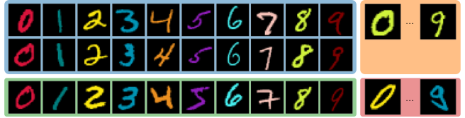
  Figure 1: Colored MNIST

  Table 1: Color Summary

  4Class	0	1	2	3	4	5	6	7	8	9
  R	0.8627451	0	0.99215686	0	0.929411765	0.568627451	0.274509804	0.980392157	0.823529412	0.501960784
  G	0.07843137	0.50196078	0.91372549	0.58431373	0.568627451	0.117647059	0.941176471	0.77254902	0.960784314	0
  B	0.23529412	0.50196078	0.0627451	0.71372549	0.129411765	0.737254902	0.941176471	0.733333333	0.235294118	0
  4

• Colored MNIST (Nam et al. 2020; Kim, Lee, and Choo 2021; Lee et al. 2021) Colored MNIST is a variant of the well-known handwritten digit dataset. This dataset is generated by injecting colors as follows: we pick ten different colors, $c_{0},...,c_{9}$, and color $1-\alpha$ samples of each class with $c_{i}$ colors where $i=y$, and the rest are colored $c_{j}$ where uniformly chosen $j\neq y$. The main objective of this task is to classify the digit shape while colors are highly correlated. For injecting variance of colors, we add variance from $c_{i}+v\sim\mathcal{N}(0,0.01^{2})$. Examples are described in Figure 1 and the picked colors are in Table 1

  

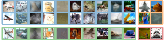
  Figure 2: Corrupted CIFAR

  Table 2: Color Summary

  4Class	0	1	2	3	4	5	6	7	8	9
  Corruption	Snow	Frost	Fog	Brightness	Contrast	Spatter	Elastic	JPEG	Pixelate	Saturate
  4

• Corrupted CIFAR (Nam et al. 2020; Lee et al. 2021) This dataset comes from the conventional CIFAR dataset. In this dataset, we focus on two attributes: object and corruption. Similar to the Colored MNIST, we select corruption types, such as $c_{0}$=blur,…, $c_{9}$=snow. $1-\alpha\%$ samples of each class are corrupted with $c_{i}$ where $i=y$. The rest samples are blurred uniformly random samples $c_{j}$ where $j\neq y$. Examples are in Figure 2 and the utilized corruptions are in Table 2.

  

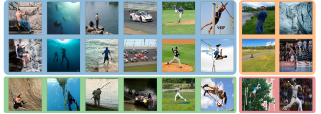
  Figure 3: Biased Action Recognition

• BAR (Nam et al. 2020) BAR dataset has totally six action categoris: e.g., racing, vaulting, climbing. Different with Colored MNIST and Corrupted CIFAR datasets, it does not contain manually injected bias attributes, i.e., it utilizes bias raw images. This dataset has two attributes: action and background. Each class has its own biased background. For example, almost all climbing action class images are taken against cliff, while only a few samples are taken against ice-cliff.

  

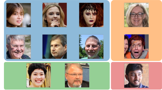
  Figure 4: Biased FFHQ

• BFFHQ (Kim, Lee, and Choo 2021; Lee et al. 2021) BFFHQ is manually subsampled dataset from FFHQ facial images. We focus on two attributes of this dataset: gender and age. Similar with BAR dataset, we do not inject manual bias attribute. The target attribute is gender when bias the bias attribute is age. The number of classes of this benchmark is binary; i.e., Male and Female. Almost male samples are old (age ranging from 40 to 59), while female samples are young (age ranging from 10 to 29). Bias-conflicting samples are opposite; (male young) and (female old).

Label flipping

We generate noisy labels by flipping the labels symmetrically, as mentioned in the main paper. Label flipping rule is as follows: (1) Select $\eta\%$ samples (2) Select new label $y$ uniformly $\{0,...,C\}$. Note that, new label $y$ can contains ground truth label.

B.3 Backbone network

Simple-Conv-Net.  We report Simple convolutional networks for Colored MNIST by PyTorch code as follows:

(conv1): Conv2d(3, 8, kernel_size=(4, 4), stride=(1, 1))
(bn1): BatchNorm2d(8, eps=1e-05, momentum=0.1, affine=True, track_running_stats=True)
(relu1): ReLU()
(dropout1): Dropout(p=0.5, inplace=False)
(avgpool1): AvgPool2d(kernel_size=2, stride=2, padding=0)
(conv2): Conv2d(8, 32, kernel_size=(4, 4), stride=(1, 1))
(bn2): BatchNorm2d(32, eps=1e-05, momentum=0.1, affine=True, track_running_stats=True)
(relu2): ReLU()
(dropout2): Dropout(p=0.5, inplace=False)
(avgpool2): AvgPool2d(kernel_size=2, stride=2, padding=0)
(conv3): Conv2d(32, 64, kernel_size=(4, 4), stride=(1, 1))
(relu3): ReLU()
(bn3): BatchNorm2d(64, eps=1e-05, momentum=0.1, affine=True, track_running_stats=True)
(dropout3): Dropout(p=0.5, inplace=False)
(avgpool3): AdaptiveAvgPool2d(output_size=(1, 1))
(fc): Linear(in_features=64, out_features=$num_class, bias=True)

ResNet18 pre-trained on ImageNet.  Except for Colored MNIST benchmark, we use pretrained ResNet18. This network is known that pre-trained using ImageNet. We obtain the parameters from torchvision library.

Table 3: Hyperparameter search spaces

4Algorithm	Name	Candidate
Common	LR	$\{0.1,0.01,0.001,0.0001\}$
	Batch size	$\{32,64,128,256\}$
	LR Decay	$\{1,0.1,0.01,0.001,0.0001\}$
	Lr decay step	$\{20,30,40\}$
	Momentum	$\{0.1,0.3,0.5,0.7,0.9\}$
	weight decay	$\{0.0,0.1,0.01,0.001,0.0001\}$
LfF	$q$	$\{0.1,0.5,0.7,0.9\}$
	$\alpha$	$\{0.01,0.1,0.5,0.7,0.9,0.99\}$
JTT	bias epochs	$\{1,10,20,50,100\}$
	$\lambda_{up}$	$\{1.,10.,20.,50.,100.\}$
Disen	$\alpha$	$\{0.01,0.1,0.5,0.7,0.9,0.99\}$
	$q$	$\{0.01,0.1,0.5,0.7,0.9,0.99\}$
	warmup	$\{0,10,20\}$
	$\lambda_{dis}$	$\{1,10,30\}$
	$\lambda_{swap}$	$\{1,10,30\}$
SCE	$\alpha$	$\{0.01,0.1,0.5,0.7,0.9,0.99\}$
	$\beta$	$\{1.0,0.5,0.7\}$
GCE	$q$	$\{0.1,0.3,0.5,0.7,0.9\}$
ELR+	$\lambda$	$\{1,3,5,7\}$
	$\beta$	$\{0.7,0.9\}$
	warmup	$\{0,10,30\}$
	ema $\alpha$	$\{0.9,0.99,0.997\}$
	ema step	$\{30000,40000,50000\}$
	mixup $\alpha$	$\{0.5,1.0,2.0,5.0\}$
	coef step	$\{0,100,1000\}$
AUM	Percentile	$\{1,10,30,50,99\}$
Co-teaching	num gradual	$\{0,2,5,10\}$
	forget rate	$\{0.1,0.3,0.5,0.9\}$
DivideMix	$\alpha$	$\{0.5,1.0,2.0,5.0\}$
	$\lambda_{u}$	$\{0,0.5,1,15,25\}$
	$p_{threshold}$	$\{0.1,0.3,0.5,0.7\}$
	warmup	$\{0,5,10\}$
	$T$	$\{0.1,0.5\}$
f-DivideMix	$\alpha$	$\{0.5,1.0,2.0,5.0\}$
	$\lambda_{u}$	$\{0,0.5,1,15,25\}$
	$p_{threshold}$	$\{0.1,0.3,0.5,0.7\}$
	warmup	$\{0,5,10\}$
	$T$	$\{0.1,0.5\}$
DENEB	$p_{threshold}$	$\{0.1,0.3,0.5,0.7,0.9\}$
	warmup	$\{0,5,10\}$
	$\tau$	$\{0.1,0.5,0.9,1.0,2.0,5.0,10.0\}$
4

Table 4: Hyperparameters for DENEB

4Benchmark	Type	$p_{threshold}$	$\tau$	$e_{w}$	$q$	Augmentation
CMNIST	$(\alpha=1\%,\eta=10\%)$	0.1	1.0	5	0.5	N/A
CMNIST	$(\alpha=5\%,\eta=50\%)$	0.9	2.0	5	0.7	N/A
CCIFAR	$(\alpha=1\%,\eta=10\%)$	0.9	10.0	5	0.3	RandomCrop(32,padding=4),RandomHorizontalFlip, Normalize((0.4914, 0.4822, 0.4465), (0.2023, 0.1994, 0.2010))
CCIFAR	$(\alpha=5\%,\eta=50\%)$	0.7	10.0	10	0.3	RandomCrop(32,padding=4),RandomHorizontalFlip, Normalize((0.4914, 0.4822, 0.4465), (0.2023, 0.1994, 0.2010))
BAR	$(\eta=10\%)$	0.5	1.0	10	0.7	Normalize((0.4914, 0.4822, 0.4465), (0.2023, 0.1994, 0.2010))
BFFHQ	$(\eta=10\%)$	0.5	1.0	10	0.7	RandomCrop(128,padding=4),Normalize((0.4914, 0.4822, 0.4465), (0.2023, 0.1994, 0.2010))
4

B.4 Hyperparameter tuning

Under our experiment, we searched best model under following search space in Table 3. Common hyperparameters, such as Learning rate, Batch size, LR decay rate, are shared for all algorithms. Since all algorithms have different hyper-parameters, we tune with $30$ trials for fair comparison. Hyperparameter tuning was conducted based on ASHAScheduler, efficient hyperparameter tuning module supported by official Ray (Liaw et al. 2018). We select the best validation accuracy model among all candidates.

Implementation details for DENEB  We summarize the hyperparameters for training DENEB for each benchmark. Detail parameters are in Table 4. These parameters are also obtained by following the hyper-parameter tuning rule.

Appendix C Experimental Settings for Section 3 and 4

C.1 Implementation for Section 3

To see the impact of the noisy labels, we observe how peformances are degraded when the labels are corrupted, as in Section 3.

Label-based implementation.  To check how the label-based approaches performs when noisy labels are injected, we test three baselines (Nam et al. 2020; Lee et al. 2021; Liu et al. 2021). For all baselines, we clone the official codes from their github site. Also, we download datasets as instructed in the site. After then, we only modify the dataloader part of the code for injecting noisy labels. Hyperparameters and running commands are exactly followed as in the instructions of all algorithms.

Label-free implementation.  To see the impact of label-free method, we utilize entropy score. Here, we summarize our entropy based approach which is composed of three steps. First, we train the biased model based on GCE with parameter $q=0.7$. This is similar with LfF and Disen. After fully train the biased model, we extract per-sample entropy. Based on the computed entropy, we obtain sampling probability of each sample, and run the stage 3 of DENEB.

C.2 Implenetation for Section 4

To see the impact of denoising on DBwNL dataset, we run five denoising algorithms. Except for AUM, all algorithms are online-manner. Therefore, we report the cleansing result at the end of training phase. For example, when we run the DivideMix with $100$ epochs, we extract division results after training $100$ epoch. Furthermore, to see the case when we can emphasize bias-conflicting samples, we multiply $\times 50$ for the bias-conflicting samples, regardless of it is noisy labels or not.

C.3 Other case study in Section 3 and 4

To verify our findings, we additionally offer the other cases. We change $\alpha$ and $\eta$. As in Figure 5, previous label-based approaches have entangled

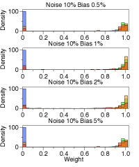
(a) LfF (Nam et al. 2020)

(b) JTT (Liu et al. 2021)

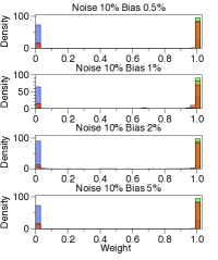
(c) Disen (Lee et al. 2021)

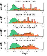
(d) Entropy

Figure 5: Score histogram of each methodology. As LfF and Disen operate online, we report the weight histogram right after the last epoch of training. Except for the Entropy case, LfF, JTT, and Disen shows entangled histograms between (noisy, aligned), (clean, conflicting), and (noisy, conflicting). By contrast, the histogram of entropy case indicates that it is clustered not according to label corruption but bias.

Appendix D Computation Resources

For all experiments, we utilized NVIDIA TITAN Xp GPUs and Intel Xeon CPU E5-2630 v4 CPU cores. $252$Gb RAM memory was available but, we partially utilized it. For Colored MNIST and Corrupted CIFAR cases, we use only one GPU. On the other hand, we use 4 GPUs for BAR and BFFHQ benchmarks. We summarize training time of CMNIST for each entity in Table 5.

Table 5: Color Summary

4Step	Step 1	Step 2	Step3
Training time	9m 3s	5s	6m 12s
Vanilla	5m 59s
4

References

- Agarap (2018) Agarap, A. F. 2018. Deep learning using rectified linear units (relu). arXiv preprint arXiv:1803.08375.
- Ahn and Yun (2021) Ahn, S.; and Yun, S.-Y. 2021. Mitigating Dataset Bias Using Per-Sample Gradients From A Biased Classifier.
- Alvi, Zisserman, and Nellåker (2018) Alvi, M.; Zisserman, A.; and Nellåker, C. 2018. Turning a blind eye: Explicit removal of biases and variation from deep neural network embeddings. In Proceedings of the European Conference on Computer Vision (ECCV), 0–0.
- Bahng et al. (2020) Bahng, H.; Chun, S.; Yun, S.; Choo, J.; and Oh, S. J. 2020. Learning de-biased representations with biased representations. In International Conference on Machine Learning, 528–539. PMLR.
- Bahri, Jiang, and Gupta (2020) Bahri, D.; Jiang, H.; and Gupta, M. 2020. Deep k-nn for noisy labels. In International Conference on Machine Learning, 540–550. PMLR.
- Berthelot et al. (2019) Berthelot, D.; Carlini, N.; Goodfellow, I.; Papernot, N.; Oliver, A.; and Raffel, C. A. 2019. Mixmatch: A holistic approach to semi-supervised learning. Advances in Neural Information Processing Systems, 32.
- Cao et al. (2020) Cao, K.; Chen, Y.; Lu, J.; Arechiga, N.; Gaidon, A.; and Ma, T. 2020. Heteroskedastic and imbalanced deep learning with adaptive regularization. arXiv preprint arXiv:2006.15766.
- Cao et al. (2019) Cao, K.; Wei, C.; Gaidon, A.; Arechiga, N.; and Ma, T. 2019. Learning imbalanced datasets with label-distribution-aware margin loss. Advances in neural information processing systems, 32.
- Creager, Jacobsen, and Zemel (2021) Creager, E.; Jacobsen, J.-H.; and Zemel, R. 2021. Environment inference for invariant learning. In International Conference on Machine Learning, 2189–2200. PMLR.
- Darlow, Jastrzkebski, and Storkey (2020) Darlow, L.; Jastrzkebski, S.; and Storkey, A. 2020. Latent Adversarial Debiasing: Mitigating Collider Bias in Deep Neural Networks. arXiv preprint arXiv:2011.11486.
- Geirhos et al. (2018) Geirhos, R.; Rubisch, P.; Michaelis, C.; Bethge, M.; Wichmann, F. A.; and Brendel, W. 2018. ImageNet-trained CNNs are biased towards texture; increasing shape bias improves accuracy and robustness. In International Conference on Learning Representations.
- Ghosh, Kumar, and Sastry (2017) Ghosh, A.; Kumar, H.; and Sastry, P. 2017. Robust loss functions under label noise for deep neural networks. In Proceedings of the AAAI conference on artificial intelligence, volume 31.
- Goodfellow et al. (2014) Goodfellow, I.; Pouget-Abadie, J.; Mirza, M.; Xu, B.; Warde-Farley, D.; Ozair, S.; Courville, A.; and Bengio, Y. 2014. Generative adversarial nets. Advances in neural information processing systems, 27.
- Goyal et al. (2020) Goyal, A.; Yang, K.; Yang, D.; and Deng, J. 2020. Rel3D: A Minimally Contrastive Benchmark for Grounding Spatial Relations in 3D. Advances in Neural Information Processing Systems, 33.
- Goyal et al. (2017) Goyal, Y.; Khot, T.; Summers-Stay, D.; Batra, D.; and Parikh, D. 2017. Making the v in vqa matter: Elevating the role of image understanding in visual question answering. In Proceedings of the IEEE Conference on Computer Vision and Pattern Recognition, 6904–6913.
- Han et al. (2018) Han, B.; Yao, Q.; Yu, X.; Niu, G.; Xu, M.; Hu, W.; Tsang, I.; and Sugiyama, M. 2018. Co-teaching: Robust training of deep neural networks with extremely noisy labels. Advances in neural information processing systems, 31.
- He et al. (2017) He, K.; Gkioxari, G.; Dollár, P.; and Girshick, R. 2017. Mask r-cnn. In Proceedings of the IEEE international conference on computer vision, 2961–2969.
- He et al. (2016) He, K.; Zhang, X.; Ren, S.; and Sun, J. 2016. Deep residual learning for image recognition. In Proceedings of the IEEE conference on computer vision and pattern recognition, 770–778.
- Hendrycks and Dietterich (2018) Hendrycks, D.; and Dietterich, T. G. 2018. Benchmarking neural network robustness to common corruptions and surface variations. arXiv preprint arXiv:1807.01697.
- Hendrycks et al. (2018) Hendrycks, D.; Mazeika, M.; Wilson, D.; and Gimpel, K. 2018. Using trusted data to train deep networks on labels corrupted by severe noise. Advances in neural information processing systems, 31.
- Idrissi et al. (2022) Idrissi, B. Y.; Arjovsky, M.; Pezeshki, M.; and Lopez-Paz, D. 2022. Simple data balancing achieves competitive worst-group-accuracy. In Conference on Causal Learning and Reasoning, 336–351. PMLR.
- Ioffe and Szegedy (2015) Ioffe, S.; and Szegedy, C. 2015. Batch normalization: Accelerating deep network training by reducing internal covariate shift. In International conference on machine learning, 448–456. PMLR.
- Kim et al. (2019) Kim, B.; Kim, H.; Kim, K.; Kim, S.; and Kim, J. 2019. Learning not to learn: Training deep neural networks with biased data. In Proceedings of the IEEE Conference on Computer Vision and Pattern Recognition, 9012–9020.
- Kim, Lee, and Choo (2021) Kim, E.; Lee, J.; and Choo, J. 2021. Biaswap: Removing dataset bias with bias-tailored swapping augmentation. In Proceedings of the IEEE/CVF International Conference on Computer Vision, 14992–15001.
- Kim et al. (2021) Kim, T.; Ko, J.; Choi, J.; Yun, S.-Y.; et al. 2021. FINE Samples for Learning with Noisy Labels. Advances in Neural Information Processing Systems, 34.
- Le Bras et al. (2020) Le Bras, R.; Swayamdipta, S.; Bhagavatula, C.; Zellers, R.; Peters, M.; Sabharwal, A.; and Choi, Y. 2020. Adversarial filters of dataset biases. In International Conference on Machine Learning, 1078–1088. PMLR.
- Lee et al. (2021) Lee, J.; Kim, E.; Lee, J.; Lee, J.; and Choo, J. 2021. Learning debiased representation via disentangled feature augmentation. Advances in Neural Information Processing Systems, 34.
- Lee et al. (2019) Lee, K.; Lee, K.; Shin, J.; and Lee, H. 2019. Network Randomization: A Simple Technique for Generalization in Deep Reinforcement Learning. In International Conference on Learning Representations.
- Li, Socher, and Hoi (2019) Li, J.; Socher, R.; and Hoi, S. C. 2019. DivideMix: Learning with Noisy Labels as Semi-supervised Learning. In International Conference on Learning Representations.
- Li, Li, and Vasconcelos (2018) Li, Y.; Li, Y.; and Vasconcelos, N. 2018. Resound: Towards action recognition without representation bias. In Proceedings of the European Conference on Computer Vision (ECCV), 513–528.
- Li and Vasconcelos (2019) Li, Y.; and Vasconcelos, N. 2019. Repair: Removing representation bias by dataset resampling. In Proceedings of the IEEE Conference on Computer Vision and Pattern Recognition, 9572–9581.
- Liaw et al. (2018) Liaw, R.; Liang, E.; Nishihara, R.; Moritz, P.; Gonzalez, J. E.; and Stoica, I. 2018. Tune: A Research Platform for Distributed Model Selection and Training. arXiv preprint arXiv:1807.05118.
- Liu et al. (2021) Liu, E. Z.; Haghgoo, B.; Chen, A. S.; Raghunathan, A.; Koh, P. W.; Sagawa, S.; Liang, P.; and Finn, C. 2021. Just train twice: Improving group robustness without training group information. In International Conference on Machine Learning, 6781–6792. PMLR.
- Liu et al. (2020) Liu, S.; Niles-Weed, J.; Razavian, N.; and Fernandez-Granda, C. 2020. Early-learning regularization prevents memorization of noisy labels. Advances in neural information processing systems, 33: 20331–20342.
- Lukasik et al. (2020) Lukasik, M.; Bhojanapalli, S.; Menon, A.; and Kumar, S. 2020. Does label smoothing mitigate label noise? In International Conference on Machine Learning, 6448–6458. PMLR.
- McDuff et al. (2019) McDuff, D.; Ma, S.; Song, Y.; and Kapoor, A. 2019. Characterizing bias in classifiers using generative models. In Advances in Neural Information Processing Systems, 5404–5415.
- Mirzasoleiman, Cao, and Leskovec (2020) Mirzasoleiman, B.; Cao, K.; and Leskovec, J. 2020. Coresets for robust training of neural networks against noisy labels. arXiv preprint arXiv:2011.07451.
- Nam et al. (2020) Nam, J.; Cha, H.; Ahn, S.; Lee, J.; and Shin, J. 2020. Learning from failure: De-biasing classifier from biased classifier. Advances in Neural Information Processing Systems, 33: 20673–20684.
- Nicholson, Sheng, and Zhang (2016) Nicholson, B.; Sheng, V. S.; and Zhang, J. 2016. Label noise correction and application in crowdsourcing. Expert Systems with Applications, 66: 149–162.
- Pleiss et al. (2020) Pleiss, G.; Zhang, T.; Elenberg, E.; and Weinberger, K. Q. 2020. Identifying mislabeled data using the area under the margin ranking. Advances in Neural Information Processing Systems, 33: 17044–17056.
- Ramaswamy, Kim, and Russakovsky (2021) Ramaswamy, V. V.; Kim, S. S.; and Russakovsky, O. 2021. Fair attribute classification through latent space de-biasing. In Proceedings of the IEEE/CVF Conference on Computer Vision and Pattern Recognition, 9301–9310.
- Ren et al. (2018) Ren, M.; Zeng, W.; Yang, B.; and Urtasun, R. 2018. Learning to reweight examples for robust deep learning. In International conference on machine learning, 4334–4343. PMLR.
- Singh et al. (2020) Singh, K. K.; Mahajan, D.; Grauman, K.; Lee, Y. J.; Feiszli, M.; and Ghadiyaram, D. 2020. Don’t Judge an Object by Its Context: Learning to Overcome Contextual Bias. In Proceedings of the IEEE/CVF Conference on Computer Vision and Pattern Recognition, 11070–11078.
- Sohoni et al. (2020) Sohoni, N.; Dunnmon, J.; Angus, G.; Gu, A.; and Ré, C. 2020. No subclass left behind: Fine-grained robustness in coarse-grained classification problems. Advances in Neural Information Processing Systems, 33: 19339–19352.
- Srivastava et al. (2014) Srivastava, N.; Hinton, G.; Krizhevsky, A.; Sutskever, I.; and Salakhutdinov, R. 2014. Dropout: a simple way to prevent neural networks from overfitting. The journal of machine learning research, 15(1): 1929–1958.
- Tartaglione, Barbano, and Grangetto (2021) Tartaglione, E.; Barbano, C. A.; and Grangetto, M. 2021. EnD: Entangling and Disentangling deep representations for bias correction. In Proceedings of the IEEE/CVF Conference on Computer Vision and Pattern Recognition, 13508–13517.
- Teney et al. (2021) Teney, D.; Abbasnejad, E.; Lucey, S.; and Hengel, A. v. d. 2021. Evading the Simplicity Bias: Training a Diverse Set of Models Discovers Solutions with Superior OOD Generalization. arXiv preprint arXiv:2105.05612.
- Veit et al. (2017) Veit, A.; Alldrin, N.; Chechik, G.; Krasin, I.; Gupta, A.; and Belongie, S. 2017. Learning from noisy large-scale datasets with minimal supervision. In Proceedings of the IEEE conference on computer vision and pattern recognition, 839–847.
- Wang et al. (2018) Wang, H.; He, Z.; Lipton, Z. C.; and Xing, E. P. 2018. Learning Robust Representations by Projecting Superficial Statistics Out. In International Conference on Learning Representations.
- Wang et al. (2019) Wang, Y.; Ma, X.; Chen, Z.; Luo, Y.; Yi, J.; and Bailey, J. 2019. Symmetric cross entropy for robust learning with noisy labels. In Proceedings of the IEEE/CVF International Conference on Computer Vision, 322–330.
- Wu et al. (2020) Wu, P.; Zheng, S.; Goswami, M.; Metaxas, D.; and Chen, C. 2020. A topological filter for learning with label noise. Advances in neural information processing systems, 33: 21382–21393.
- Yu et al. (2019) Yu, X.; Han, B.; Yao, J.; Niu, G.; Tsang, I.; and Sugiyama, M. 2019. How does disagreement help generalization against label corruption? In International Conference on Machine Learning, 7164–7173. PMLR.
- Yu et al. (2018) Yu, X.; Liu, T.; Gong, M.; and Tao, D. 2018. Learning with biased complementary labels. In Proceedings of the European conference on computer vision (ECCV), 68–83.
- Zhang, Lopez-Paz, and Bottou (2022) Zhang, J.; Lopez-Paz, D.; and Bottou, L. 2022. Rich Feature Construction for the Optimization-Generalization Dilemma. arXiv preprint arXiv:2203.15516.
- Zhang et al. (2022) Zhang, M.; Sohoni, N. S.; Zhang, H. R.; Finn, C.; and Ré, C. 2022. Correct-N-Contrast: A Contrastive Approach for Improving Robustness to Spurious Correlations. arXiv preprint arXiv:2203.01517.
- Zhang and Sabuncu (2018) Zhang, Z.; and Sabuncu, M. 2018. Generalized cross entropy loss for training deep neural networks with noisy labels. Advances in neural information processing systems, 31.
- Zhang et al. (2020) Zhang, Z.; Zhang, H.; Arik, S. O.; Lee, H.; and Pfister, T. 2020. Distilling effective supervision from severe label noise. In Proceedings of the IEEE/CVF Conference on Computer Vision and Pattern Recognition, 9294–9303.