On the strong local potential limit

Abstract

Finite, bound, many-body systems, where the interaction operator, $V=\sum v_{ij}$, is local and happens to strongly dominate the kinetic energy operator, $T=\sum t_{i}$, display a classical limit from diagonalizing $V$ alone, hence a clear picture of interparticle correlations, such as steric blocking emerges. This limit exhibits intrinsic symmetries and also fluctuations from mass formulae. The present work investigates how such emergent symmetries and fluctuations might be extrapolated to physical situations where $T$ is reinstated.

PACS numbers: 13.75.Cs,13.85.-t, 21.60.Cs

1 Introduction and basic formalism

Consider a system of a finite number $A$ of identical constituents with Hamiltonian, $H=T+V$, where $T=\sum_{i=1}^{A}p_{i}^{2}/(2m)$ is the kinetic energy and $V=\sum_{i<j}v\left(\left|\mathbf{r}_{i}-\mathbf{r}_{j}\right|\right)+v_{cm}$. Here, $v$ is the local two-body potential, which, for nuclear physics for instance, is the nucleon-nucleon interaction. (There are many formulations; see Refs. Vo65,Go70,Ma87,Ma89,Wi95 for representative examples.) The elementary mass is denoted by $m$, and $\mathbf{p}_{i}\equiv\left\{p_{xi},p_{yi},p_{zi}\right\}$ and $\mathbf{r}_{i}\equiv\left\{x_{i},y_{i},z_{i}\right\}$ are the momentum and position of particle $i$, respectively. Finally the term, $v_{cm}=Am\omega^{2}R^{2}/2$, where $\mathbf{R}=A^{-1}\sum_{i=1}^{A}\mathbf{r}_{i}\equiv\left\{X,Y,Z\right\}$, factorizes the center-of-mass (cm) in a spherical, Gaussian packet at the origin of the laboratory frame, with energy $\frac{3}{2}\hbar\omega$, in order to remove translational degeneracy. Without such a term, frequently omitted in the literature, the ground state of $H$ would not be square integrable, because of a zero momentum plane wave for its center-of-mass.

Since $T$ is a one-body operator, one usually replaces $V$ by a mean-field potential or a DFT one[6], $U=\sum_{i=1}^{A}u_{i}$, to take advantage of the easy diagonalization of $T+U$. One then reinstates, as much as possible, correlations brought by $V-U$. However, in the present work, we exchange the roles of $V$ and $T$, whereupon we shall show that it makes sense to first diagonalize $V$ and write $H=V+\lambda T$, where $\lambda$ is a small dimensionless constant such that $\lambda T$ represents a weak perturbation. (See Refs. Gi82,Gi78,Gi84, for the virtues of positive (semi-)definite operators, such as $T$, as perturbations.)

In many cases of physical interest, the physical system under study can be modeled as driven by a two-body interaction that can be taken as a local, finite-range, rotationally invariant potential, $v_{ij}=v\left(\left|\mathbf{r}_{i}-\mathbf{r}_{j}\right|\right)$, with a short range repulsion, sometimes even a hard core, and a pocket of attraction at mid-range. The presence or absence of a tail of $v_{ij}$ will not be important for our arguments in the following. What the diagonalization of $V$ alone will bring is a clear picture of the role of steric crowding, a familiar concept in classical physics, but a much less straightforward concept for the analysis of full-fledged wave functions, quantum mechanically, given that sharp positions are washed out by $T$. But we shall show that this concept of crowding can remain of some utility.

At the “strong $V$” limit used herein, it makes no difference whether the $A$ elements of our system are classical or quantum (boson or fermion) objects. This stems from the observation that in the limit $\lambda\rightarrow 0$, the Hamiltonian is driven solely by the potential energy and its spectrum in this limit is continuous[7]. For the sake of pedagogy and simplicity, this work ignores spin and other complications such as isospin, Coulomb effects, and/or mixtures of two or more kinds of particles. This then allows us to investigate the emergent symmetries of the Hamiltonian classically, and from those evaluations producing a natural correspondence to quantum mechanical many-body systems. As we shall show, the purely classical limit provided by $V$ alone illustrates important properties.

The locality of $v$ provides a trivial diagonalization of the full operator $V$. Indeed, one just needs a search of distinct, classical positions, $\mathbf{s}_{i}$, and, if one wants to make correspondence with quantum mechanics, one simply needs a product of very narrow wave packets as a substitute for the product of $\delta$-functions, $\prod_{i=1}^{A}\delta(\mathbf{r}_{i}-\mathbf{s}_{i})$. Those classical positions, $\mathbf{s}_{i}$, are the set that minimizes $V$ as a classical function. Note that, when calculating $\left\langle V\right\rangle$, exchange terms driven by distinct, very narrow, wave packets are negligible. (Exchange terms strictly vanish with $\delta$-functions.) Also, because of $v_{cm}$, any optimal pattern of positions $\mathbf{s}_{i}$ will be centered at the origin of the laboratory frame. Rotational degeneracy remains, but can be handled later, by using a deformed rather than spherical $v_{cm}$, for example.

The use of classical physics to achieve this may seem counter-intuitive, but, only important at this stage, is the fact that the diagonalization of just $V$ generates symmetries and transparently illustrates, often through shells, the steric blocking[10] of particles. This also gives an intuition of irregularities in the table of binding energies when the particle number $A$ increases. (Actually, the use of $\delta$-functions can be alleviated by subtracting from $V$ a slight perturbation, $\varepsilon\,\left|\phi\rangle\langle\phi\right|$, where $\varepsilon$ is a small, positive number and $\phi$ is a broad and flat wave function in $A$ dimensions, then adding that perturbation back to $\lambda T$[7]. This technicality does not influence physics and will be understood in the following.)

That $V$ alone can induce shells and also induces mass fluctuations is an important statement. In the nuclear shell model (for example), the evidence for shells in the structure of the many-body nucleonic systems comes from the observation of the magic numbers. A single-particle basis is constructed to explain the magic numbers. That basis assumes first and foremost harmonic oscillator single-particle states which are then supplemented by angular momentum states with spin-orbit splitting, as well as isospin. Harmonic oscillators are used for the single particle wave functions for their simplicity and analyticity, making the calculations tractable. And from that basis, the shell model Hamiltonian may be diagonalized with respect to many-body configurations within that shell model basis. The inherent shell structures are an underlying assumption in that respect, and the potentials derived within the spaces involved are defined only for those spaces. Woods-Saxon functions would be more appropriate, but, as the Woods-Saxon potential cannot be solved analytically, such calculations are highly impractical. Hence, instead of assuming shell structures a priori, can there be a more natural origin of shell structure?

In Section II, we present a toy model to suggest that results from $V$ alone are likely to survive the return of $T$. Then, in Sections III, IV, and V, for the sake of pedagogy, graphical convenience and shorter computer time, we shows quite a few two-dimensional (2d) results. We then present a significant number of three-dimensional (3d) results in Sec. VI, which display an illustrative sampling set of “$V$ alone” solutions, and their symmetries and/or irregularities.

Such calculations correspond to a semirealistic situation, with mainly a trivial Volkov-like potential, made of two Gaussians (2G),

$$v\left(r_{ij}\right)=v_{\text{rep}}\exp\left[-\mu_{\text{rep}}r^{2}_{ij}\right]+v_{\text{att}}\exp\left[-\mu_{\text{att}}r^{2}_{ij}\right],$$ (1)

where $r_{ij}=\left|\mathbf{r}_{i}-\mathbf{r}_{j}\right|$ , and $v_{\text{rep}}$, $v_{\text{att}}$, $\mu_{\text{rep}}$, and $\mu_{att}$, specify the strengths and ranges of a repulsion and an attraction. Such a choice is practical for the calculation of matrix elements in a harmonic oscillator shell model basis.

Section VII presents our conclusions. And, for what follows, the units are arbitrary in all our results.

2 Toy model to study localization

It is trivial that the ground state of a 1d harmonic oscillator, with Hamiltonian, $h=p^{2}/(2\mu)+\frac{1}{2}Kx^{2}$, lies at energy $\frac{1}{2}\hbar\sqrt{K/\mu}$ with wave function $\pi^{-\frac{1}{4}}\beta^{-\frac{1}{2}}e^{-x^{2}/(2\beta^{2})}$, where the width $\beta$ relates to $\mu$ through $\beta^{2}=\hbar/\sqrt{K\mu}$. We shall investigate whether, when $\mu$ is finite and large, delocalization effects remain small, of order $1/\sqrt{\mu}$.

We set $\hbar=1$, and, in a transparent notation, the equation for relative motion reads,

$$-\frac{1}{2\mu}\frac{d^{2}\psi\left(r\right)}{dr^{2}}+\left(9e^{-9r^{2}}-e^{-r^{2}}\right)\psi\left(r\right) =\eta_{rel}\psi\left(r\right),$$

$$\psi\left(0\right) =0.$$ (2)

(Remember that the cm factorises out into a Gaussian.) We are only interested in this relative motion equation, Eq. (2), with its relative coordinate $r=\left|\mathbf{r}_{2}-\mathbf{r}_{1}\right|$, relative momentum $p_{rel}=\left|\mathbf{p}_{2}-\mathbf{p}_{1}\right|/2$ and relative mass $\mu=m/2$. An expansion of the potential from its minimum, $v_{0}=-0.51320$ at $r_{0}=0.741152$, yields the harmonic approximation of Eq.(2),

$$-\frac{1}{2\mu}\frac{d^{2}\varphi\left(r\right)}{dr^{2}}+\left[v_{0}+\frac{1}{2}\left(\frac{d^{2}v_{0}}{dr^{2}}\right)\left(r-r_{0}\right)^{2}\right]\varphi\left(r\right)=\eta_{h}\,\varphi\left(r\right),$$ (3)

where $d^{2}v_{0}/dr^{2}=10.1485$ is the second derivative of the potential at its minimum. The potential with its harmonic approximation is shown in Fig. 1. It will be instructive to compare the radial wave $\psi$ and

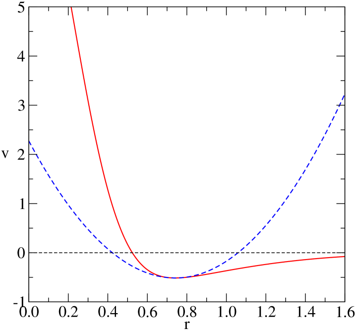
Figure 1: The toy potentials used to compare the Gaussian approximations with the full solutions. The toy potential around its minimum is portrayed by the solid line while the dashed line portrays its harmonic approximation.

the Gaussian $\varphi$, although the latter does not strictly vanish when $r=0$. But both narrow in width when $\mu$ increases. We show in Fig. 2 the Gaussians obtained when

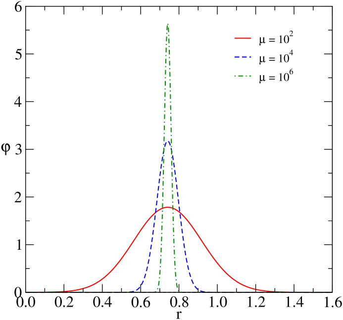
Figure 2: Narrowing Gaussians as the mass increases. The three cases shown are $\mu=10^{2}$ (solid line), $\mu=10^{4}$ (dashed line), and $\mu=10^{6}$ (dot-dashed line).

$\mu=10^{2},10^{4}$, and $10^{6}$. The narrowing of the Gaussians with increasing $\mu$ is clearly shown.

We show in Fig. 3 how close from each other the true

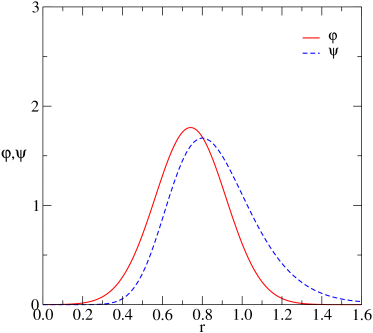
Figure 3: The case for $\mu=10^{2}$: the wave packet, the relative wave function, is denoted by the dashed line; the solid line portrays its Gaussian equivalent. The same potentials as in Fig. 1 are used.

relative function, at energy $\eta_{rel}=-0.369560$, and its Gaussian approximation, at energy $\eta_{h}=-0.353916$, are when $\mu=10^{2}$. Note that the former wave packet is slightly shifted towards greater $r$ compared to the latter. This occurs because the $v$ potential there is much less confining than the parabolic branch.

The case where $\mu=10^{4}$ is shown in Fig. 4, where the true wave

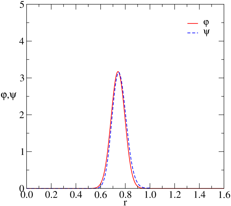
Figure 4: The case for $\mu=10^{4}$: the relative wave function is given by the dashed line, while the solid line portrays its Gaussian partner. The same potentials as in Fig. 1 are used.

packet, at energy $-0.497446$, shrinks like the harmonic one, at energy $-0.497272$, and a tiny shift remains. But then, when $\mu=10^{6}$, the wave packets are so close to each other that the shift becomes negligible (and so not shown). The localization process is at work and is driven by the scale order, $\mu^{-1/2}$.

3 Toy 2G potential for two-dimensional systems

In the following, we first use the schematic, scalar potential,

$$v_{ij}=5\exp\left[-9\left(\mathbf{r}_{i}-\mathbf{r}_{j}\right)^{2}\right]-\exp\left[-\left(\mathbf{r}_{i}-\mathbf{r}_{j}\right)^{2}\right],$$ (4)

a difference of two Gaussians (henceforth denoted as “2G”). This is displayed by the solid line in Fig. 5.

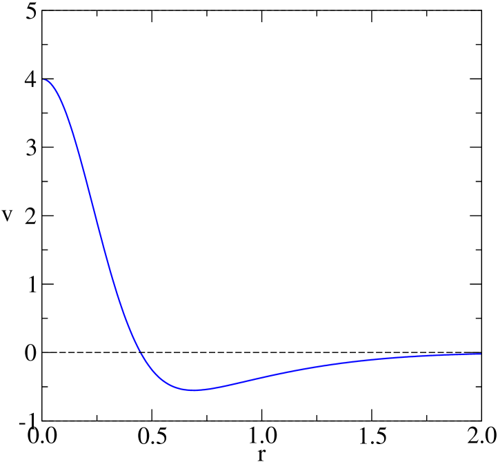
Figure 5: The toy 2G potential used in the 2d calculations.

The bottom of the 2G potential lies at $E_{2}=-0.5523$ with interparticle distance $r_{2}=0.6898$.

Such interparticle distances and bindings also give the correct results for the links of equilateral triangles, the trivial solution when $A=3$.

For the results to follow, we begin the calculation with a random distribution of the particles in a defined area (2d calculations) or volume (3d calculations later in this paper) and the two-body interaction is applied to any two particles in the system. With successive two-body interactions applied to the system, we seek the minimal energy solution, the resulting configuration of which we term the optimal configuration. Finally, the coordinates are translated such that the cm is at the origin of the coordinate system.

4 Shell structure

We begin with a nine-particle system, under the influence of the 2G potential, through to the twelve-particle system. That sequence is displayed in Figs. 6 to 9, and exhibits an increase in particle number in either the inner shell or the outer shell. This is not

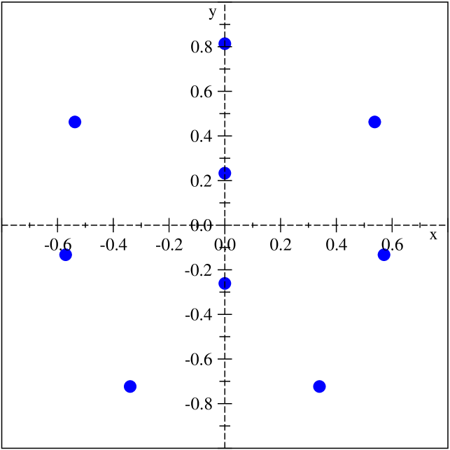
Figure 6: Optimal configuration obtained with the 2G potential for $A=9$. The energy is $-13.318$.

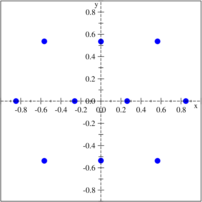
Figure 7: As for Fig. 6, but for $A=10$. The energy is $-15.807$.

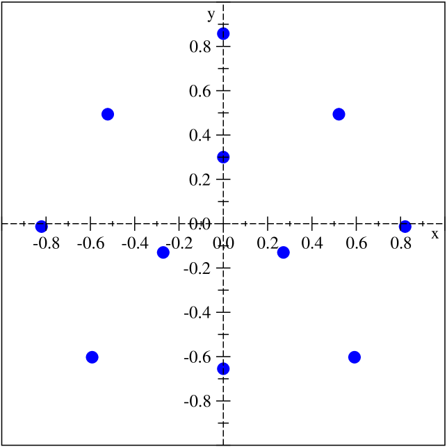
Figure 8: As for Fig. 6, but for $A=11$. The energy is $-18.620$.

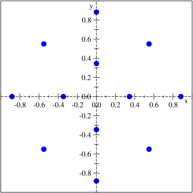
Figure 9: As for Fig. 7, but for $A=12$. The energy is $-21.457$.

entirely predictable: the evolution of the configurations to the minimal energy solution is classical. The Pauli Principle is not imposed on the system and so there is no maximum set number of particles in each shell as dictated by angular momentum quantum numbers in quantal systems. For this sequence, $9\leqslant A\leqslant 12$, the numbers in the inner shell are $2,2\left(3\right),3,4$ while those in the outer shell are $7,8\left(7\right),8,8$. The corresponding energies are $-13.318,-15.807\left(-15.774\right),-18.620,-21.457$. The anomalous case, $A=10$, is a result of a competing solution, corresponding to a very slightly excited configuration (as given in parentheses) compared to the minimal energy configuration. That excited configuration has 3 particles in the inner shell and 7 in the outer.

The existence of an alternative configuration for $A=10$ corresponding to the excited energy is not unique. It also occurs for $A=12$, whereby the excited energy configuration (for which the energy is $-21.337$) has 3 particles in the inner shell instead of 4. With that configuration there is also a breaking of symmetry; the configuration morphs from having two symmetry axes to one.

There is no doubt that the emergence of shell structure is observed at this point, although that differs from the usual behaviour where the inner shell is essentially stable and with growth occurring in the outer shell. One may speculate that the introduction of Coulomb effects may enhance the population of outer shells. The presence in Figs. 6 through 9, of quite a few quasi-alignments of particles and some parallel alignments is also noteworthy. Further, one may also conjecture that several more or less equilateral triangles are emerging. This suggests that some hexagonal crystallization may be at work.

5 Shells of many-particle systems

5.1 From two to three shells

We begin with the optimal configurations for $A=13,14$, being the minimal energy solutions for those particle numbers, as obtained using the 2G potential. Those solutions are shown in Figs. 10 and 11, respectively.

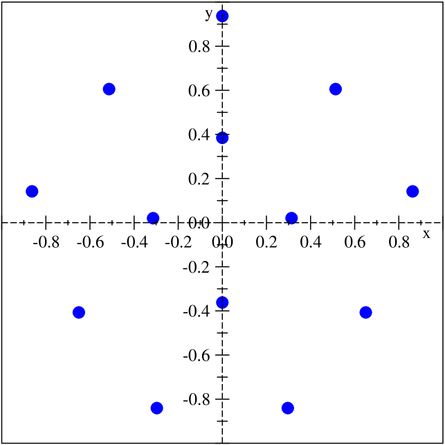
Figure 10: Optimal configuration using the 2G interaction for $A=13$. The energy is $-24.347$.

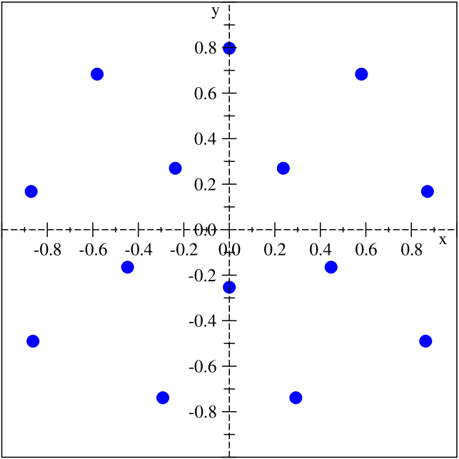
Figure 11: As for Fig. 10, but for $A=14$. The energy is $-27.298$.

With the addition of one particle, giving the $A=15$ system, one observes the emergence of a third shell, manifesting in the first instance as a particle at the centre-of-mass. This is shown in Fig. 12.

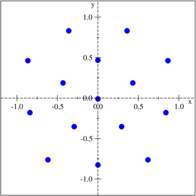
Figure 12: As for Fig. 10, but for $A=15$. The energy is $-30.378$.

This is observed also in the optimal configurations for $16\leqslant A\leqslant 19$.

The situation changes for $A=20$, as shown in Fig. 13. The innermost shell gains an additional particle, which results in there being no particle in the centre-of-mass, but two particles nearby, defining an axis of symmetry.

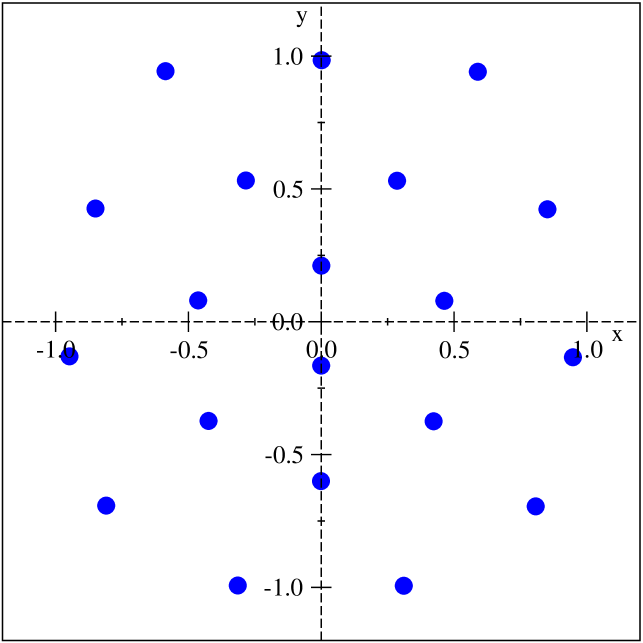
Figure 13: As for Fig. 10, but for $A=20$. The energy is $-47.628$.

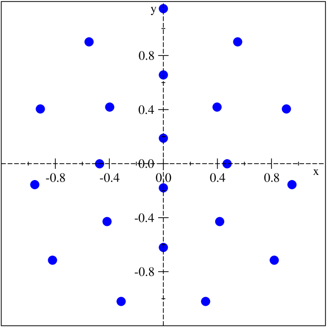
Figure 14: As for Fig. 10, but for $A=21$. The energy is $-51.331$.

From $A=20$ to $A=21$, the latter being shown in Fig 14, one observes that the addition of the particle occurs in the middle shell.

The addition of one more particle to form the $A=22$ system, shown in Fig. 15, results in a change in the innermost shell, forming a triangle, while the other two shells remain largely undisturbed.

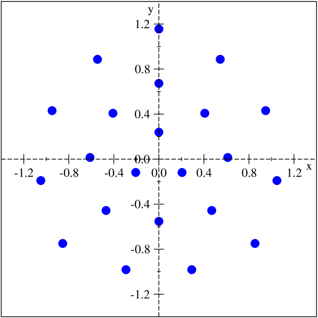
Figure 15: As for Fig. 10, but for $A=22$. The energy is $-55.083$.

The particle added to the $A=22$ system, forming the $A=23$ system as shown in Fig. 16, places that additional particle in the outer shell.

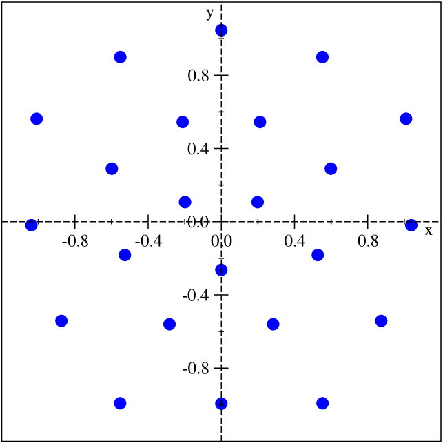
Figure 16: As for Fig. 10, but for $A=23$. The energy is $-58.993$.

It can be noted that in all cases, there exists at least one axis of symmetry.

5.2 From three to four shells and beyond

The emergence of the fourth shell occurs for $A=30$. Figs. 17 and 18 show this transition, where the $A=29$ system is the largest which exhibits three shells, with a pentagonal innermost shell, and $A=30$ showing the fourth shell, manifest as a single particle near the centre.

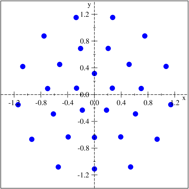
Figure 17: As for Fig. 10, but for $A=29$. The energy is $-83.933$.

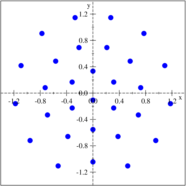
Figure 18: As for Fig. 10, but for $A=30$. The energy is $-88.357$.

The population of each shell for $A=30$ is $1,6,10,13$, proceeding from the innermost to the outermost. However, the shells are not truly distinct: there is a little ambiguity in the assigning of the number in the second shell, as one of the particles may be in the third shell. Yet that particle, on the $y$ axis, defines the shell as complete, in terms of a circular symmetry of the second shell consistent with the other shells, and so we ascribe it to the second shell. Further work is required as there is a lack of convexity in the outermost shell, and a fully convex solution may exist.

Figure 19 shows the optimal configuration of the system of 35 particles, with energy $-111.773$. This is the largest system which still has one particle, at or near the centre-of-mass, defining the innermost shell.

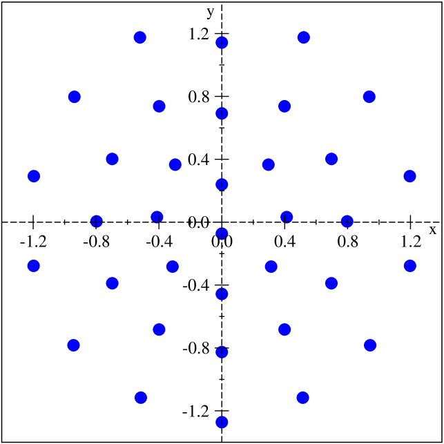
Figure 19: As for Fig. 10, but for $A=35$. The energy is $-111.773$.

The shell populations are 1, 8, 12, and 14, from the innermost to the outermost shells, respectively, with the same ambiguity in the inner shells as displayed in Fig. 18. While one may interpret the configuration as having two particles in the innermost shell and seven in the next shell, the definition of the outermost shell requiring the same average interparticle distance between all particles in that shell would favour the populations as stated with one particle only in the innermost shell.

It is in the next system, $A=36$, with energy $-116.701$, where two particles in the innermost shell become distinct. That is shown in Fig. 20.

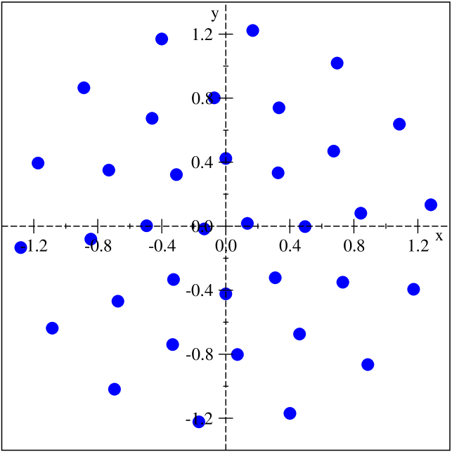
Figure 20: As for Fig. 10, but for $A=36$. The energy is $-116.701$.

The shell populations are 2, 8, 12 and 14. In this case, there are four distinct shells, but no real axis of symmetry. The particles near the $x$ axis suggest the possibility of a symmetry axis but that is not well-defined. Notice, however that the centre-of-mass turns out to be a symmetry centre of the whole pattern.

For $A=37$, for which the optimal configuration with energy $-121.706$ is shown in Fig. 21, a pair of particles in the innermost shell is still observed.

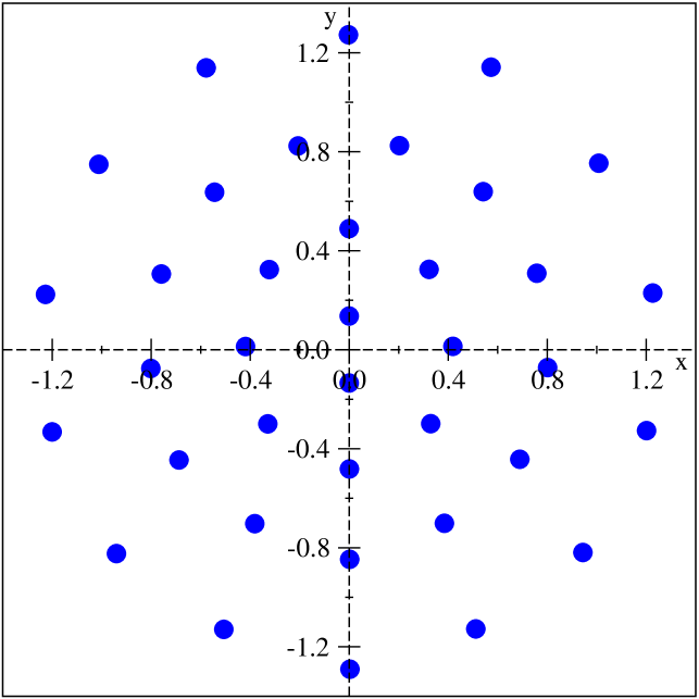
Figure 21: As for Fig. 10, but for $A=37$. The energy is $-121.706$.

The populations from the innermost to the outermost shells are 2, 8, 13, and 14. In this case, a symmetry axis is recovered.

While not displayed, we have also obtained results for $A=40$ and 41, which show more population of the innermost shells, with populations of 3 and 4, respectively, while retaining four shells overall.

We have also obtained preliminary results for the transition from four to five shells, with the transition occurring at $A=48$, showing 6 particles in the innermost shell. That is also the case for $A=49$. At $A=50$, the single particle at the centre returns, with 7 particles in the next shell. This requires further investigation.

Generally, one observes the growth of shells beginning with the innermost shell until saturation occurs, typically with five or six particles, after which the new shell emerges with a single particle at or close to the centre. The rest of the shells grow to accommodate the behaviour in the centre. This is intuitive: one expects that the particles influenced by the greatest number of interactions to be near the centre rather than the outer shells, which redistribute the populations to account accordingly. This may lead to a classical correspondence of magic numbers which, in quantal many-body systems, are attributed exclusively to angular momentum. It should be noted that these configurations display $SO(2)$ symmetry, indicating angular momentum emerges as a natural symmetry. (The analysis will be the subject of a forthcoming paper.)

6 From two to three dimensions

It is clear from the results for the optimum configurations in two dimensions that the potential [Eq. (4)] gives rise to concentric shells centred at the centre-of-mass. We now extend that to the case of three dimensions, using the potential, based on Eq. (1),

$$v_{ij}=9\exp\left[-9\left(\mathbf{r}_{i}-\mathbf{r}_{j}\right)^{2}\right]-\exp\left[-\left(\mathbf{r}_{i}-\mathbf{r}_{j}\right)^{2}\right],$$ (5)

which we denote as “2G3”, taking into account the change in steric crowding. We also, for these cases, give histograms for the distributions of the radii from the centre-of-mass of each particle to assist in illustration. As before, we begin with a random distribution of particles in a given volume, then apply the two-body 2G3 interaction to the system and allow the system to converge to the optimal, minimum energy, configuration.

We begin with the $A=15$ particle system by way of illustration. The optimal configuration obtained is shown in Fig. 22, for which the energy is $E=-38.0945$.

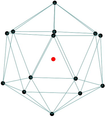
Figure 22: Optimal configuration for a system of 15 particles in 3 dimensions. The energy is $E=-38.0945$. The different colours and lines for the shells serve as a guide only: red denotes the inner shell while black denotes the outer shell.

The histogram of the radii is shown in Fig. 23. Therein, the configuration is

Figure 23: Histogram of particle radii for the $A=15$ system.

a particle at the centre surrounded by a shell of radius 0.5.

The optimal configuration for the $A=20$ system is shown in Fig. 24,

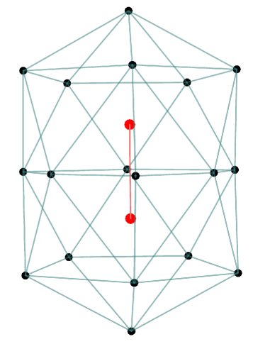
Figure 24: As for Fig. 22, but for $A=20$. The energy is $E=-61.4145$.

for which the corresponding histogram for the particle radii is given in Fig. 25.

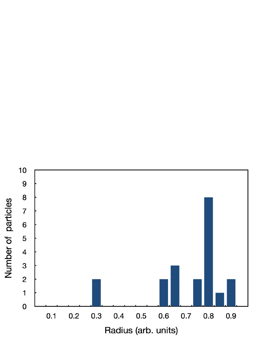
Figure 25: Histogram of particle radii for the $A=20$ system.

For the $A=20$ system, the inner shell, defined by two particles, clearly defines an axis of symmetry, and the particles in the outer shell are distributed evenly along that axis of symmetry, defining more a cylindrical shell rather than a spherical one. That is reflected in the wider distribution of radii of the particles in the outer shell as shown in Fig. 25.

Fig. 26 displays the optimal configuration for $A=40$, with the histogram of the particles’ radii shown in Fig. 27. The energy is $E=-192.6239$.

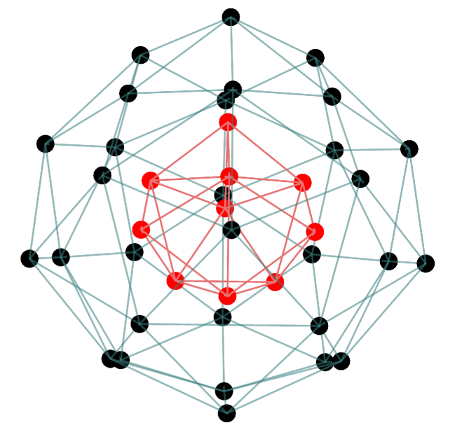
Figure 26: As for Fig. 22, but for a 40 particle system. The energy is $E=-193.6239$.

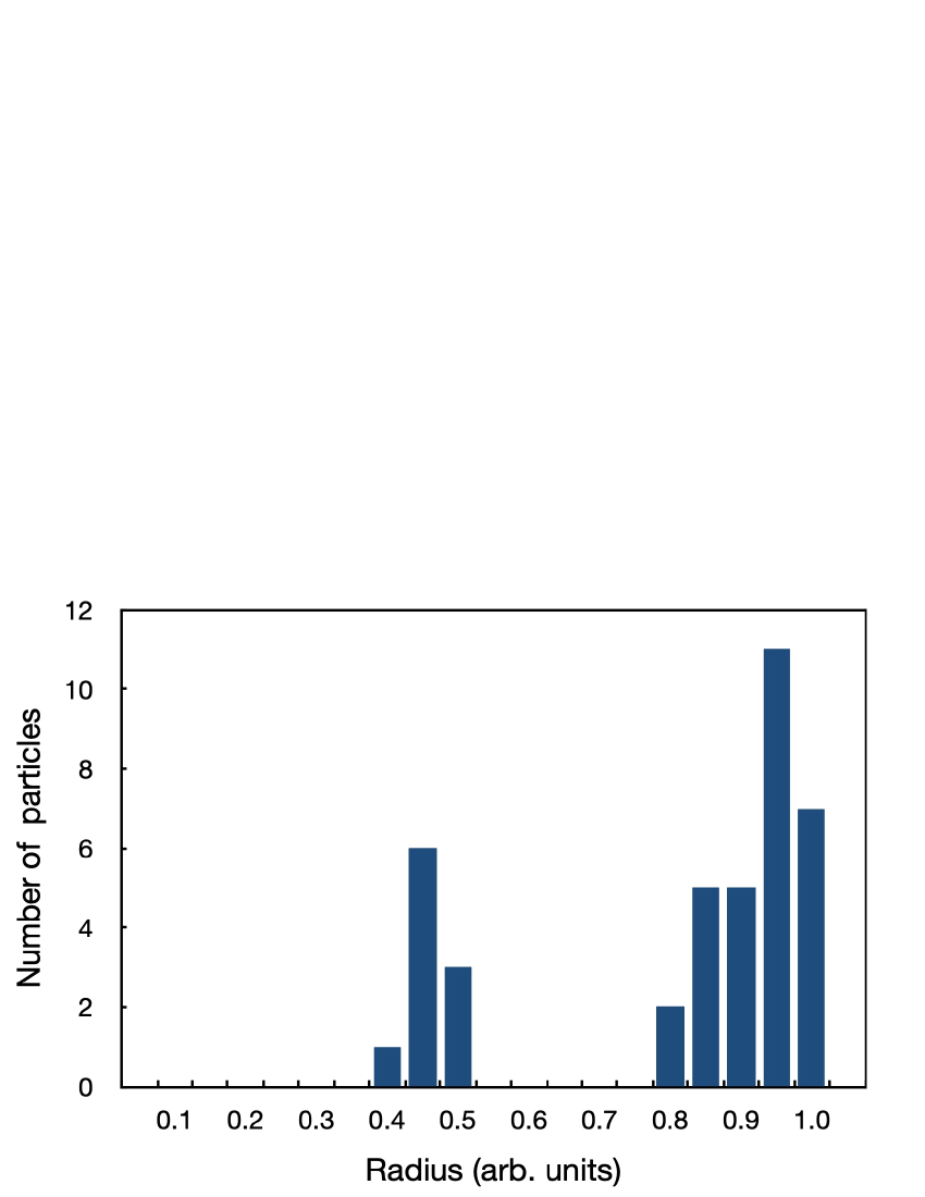
Figure 27: Histogram of particle radii for the $A=40$ system.

Again, there are two distinct concentric spherical shells in this configuration, with the radius of the outer shell roughly twice the radius of the inner one, as shown in the histogram.

The optimal configuration and histogram of the particles’ radii for the $A=60$ system are shown in Figs. 28 and 29, respectively.

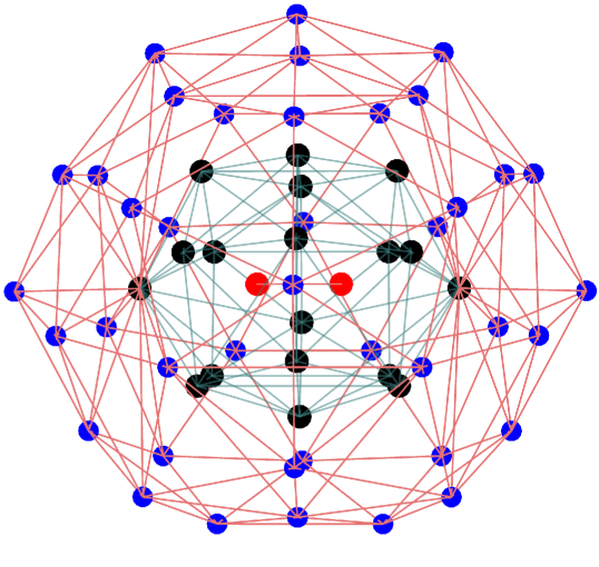
Figure 28: As for Fig. 22, but for $A=60$. The energy is $E=-374.8513$. The red and black shells denote the innermost and middle shells, respectively, while the outer shell is in blue.

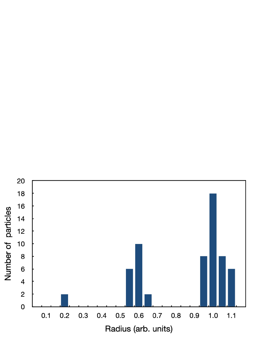
Figure 29: Histogram of particle radii for the $A=60$ system. As indicated by the spacing of the particles’ radii, this system has a configuration of three shells.

For $A=60$ there are now three distinct shells, as confirmed by the radii. The innermost shell has only two particles but with the much larger number of particles compared to $A=20$, the cylindrical symmetry is relaxed and the shells are now spherical.

Figs. 30 and 31 display the optimal configuration and the histogram of the particles’ radii for the $A=75$ system. The energy is $-538.6275$.

Figure 30: As for Fig. 28, but for the $A=75$ system. The energy is $E=-539.6275$.

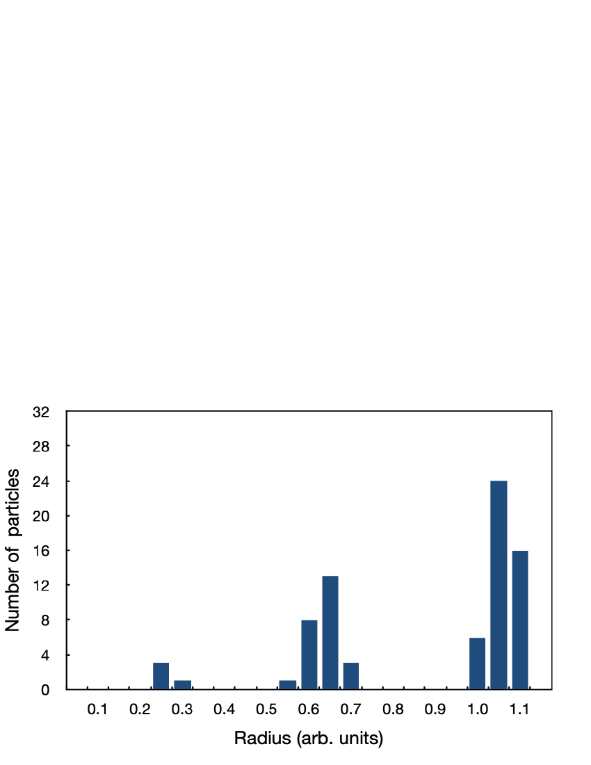
Figure 31: Histogram of the particles’ radii for the $A=75$ system.

The optimal configuration also shows three distinct shells. The innermost shell now is formed by a triangular pyramid, which entrenches the spherical symmetry of the middle and outer shells.

Similarly to the two-dimensional systems, these systems exhibit $SO(3)$ symmetry, with the increase in rank indicative of the extra dimension. Angular momentum emerges once more as a natural symmetry.

7 Conclusions

We have generated a catalogue of patterns in two dimensions of systems of identical particles that optimise the potential energy, and where the kinetic energy has been neglected. The systems were allowed to evolve classically under the action of finite-range attractive potentials with a repulsive hard core. This allowed for easy observations of symmetries and correlations. The role played by steric crowding in such features has been illustrated, with details of the interaction leading to either crystals or shells.

For the toy 2G potential, the attractive pocket is smooth and allows deviations from the strict optimal interparticle distance. Clearly, shells enforce such deviations, whether between neighbours in a shell or across neighbouring shells at distances not too far from the strict two particle optimum. Clearly, global binding then results from interactions between next-to-nearest neighbours as well as nearest neighbours.

In the case of the extension to three dimensions, with the use of the 2G3 potential, we see the generalisation of the circular symmetry of the optimal configurations in two dimensions to that of spherical symmetry in three. The only exception to that is for the two lightest systems shown, $A=15$ and $A=20$, where the axis of symmetry and the stronger repulsion of the 2G3 potential lead to cases of cylindrical symmetry. The increase in particle number relaxes that symmetry to the spherical symmetry inherent in the larger systems to allow for the uniform distribution of particles in each shell.

Given that these are classical systems, evolving dynamically under a finite-range interaction with short-range attraction and a hard repulsive core, one can postulate that the emergence of the shells stems from an average interparticle distance, as given by the relatively narrow attraction in the short-range potential. There is no actual restriction in the number of particles save for the interparticle distance aspect eventually saturating one shell and creating the next. This is unlike the quantum mechanical case of a system of fermions with angular momentum symmetry, where the number of particles in each shell is determined by the total angular momentum.

Historically, shells were understood in three dimensions from central potential theories, among which are the exactly solvable Coulomb and harmonic oscillator potentials. Mean field theories and density functional theories also lead to shells. Yet in the cases presented in this study, the shells may emerge without the introduction or use of a centered field approach. The natural next step is to introduce the kinetic energy, from which we would also expect the retention of shells, as the action of the potential would still dictate the interparticle spacing, and also to turn to quantal systems of identical particles, without and with spin. In the latter case one may investigate also pairing, and the natural observation of magic numbers, with angular momentum appearing naturally, given the spherical, or ellipsoidal symmetry observed herein.

Many cases of shell structures, including the existence of magic numbers, have been published in the physics of clusters. They are too numerous to be cited extensively and we refer here to very few of them[11, 12] only. Up to our knowledge, the majority of cluster studies have used mean field and/or density functional, centered methods. Our pure two-body approach, with its trivially simple calculations, may bring new results or easier confirmations and interpretations of results based on quantum mechanical nuclear structure models.

In short, the main result of this work is that there is no need of a one-body, centered theory to bring shells and their symmetries. Bare two-body theories, based on simple representations of finite-range, local, interactions, are sufficient and lend a more microscopic basis to the evolution of such structures and the understanding of interparticle correlations.

References

- [1] A. B. Volkov, Nucl. Phys. 74 (1965) 33.
- [2] D. Gogny, Phys. Rev. C 1 (1970) 1353.
- [3] R. Machleidt, K. Holinde and C. Elster, Phys. Rep. 149 (1987) 1.
- [4] R. Machleidt, Adv. Nucl. Phys. 19 (1989) 189.
- [5] R. B. Wiringa, V. G. J. Stoks and R. Schiavilla, Phys. Rev. C 51 (1995) 38.
- [6] W. Kohn and L. J. Sham, Phys. Rev. 140 (1965) A1133.
- [7] B. G. Giraud, Phys. Rev. C 26 (1982) 1267.
- [8] B. G. Giraud, Phys. Rev. C 17 (1978) 800.
- [9] B. G. Giraud, J. Phys. A 17 (1984) 5.
- [10] M. Grzelczak, A. Sánchez-Iglesias, H. H. Mezerji, S. Bals, J. Pérez-Juste and L. M. Liz-Martin, Nano Lett. 12 (2012) 4380.
- [11] R. G. Parr and Z. Zhou, Acc. Chem. Res. 26 (1993) 256.
- [12] M. P. Iniguez, J. A. Alonso and L. C. Balbas, Solid State Comm. 57 (1986) 85.