Spectral Feature Augmentation for Graph Contrastive Learning and Beyond

Abstract

Although augmentations (e.g., perturbation of graph edges, image crops) boost the efficiency of Contrastive Learning (CL), feature level augmentation is another plausible, complementary yet not well researched strategy. Thus, we present a novel spectral feature argumentation for contrastive learning on graphs (and images). To this end, for each data view, we estimate a low-rank approximation per feature map and subtract that approximation from the map to obtain its complement. This is achieved by the proposed herein incomplete power iteration, a non-standard power iteration regime which enjoys two valuable byproducts (under mere one or two iterations): (i) it partially balances spectrum of the feature map, and (ii) it injects the noise into rebalanced singular values of the feature map (spectral augmentation). For two views, we align these rebalanced feature maps as such an improved alignment step can focus more on less dominant singular values of matrices of both views, whereas the spectral augmentation does not affect the spectral angle alignment (singular vectors are not perturbed). We derive the analytical form for: (i) the incomplete power iteration to capture its spectrum-balancing effect, and (ii) the variance of singular values augmented implicitly by the noise. We also show that the spectral augmentation improves the generalization bound. Experiments on graph/image datasets show that our spectral feature augmentation outperforms baselines, and is complementary with other augmentation strategies and compatible with various contrastive losses.

1 Introduction

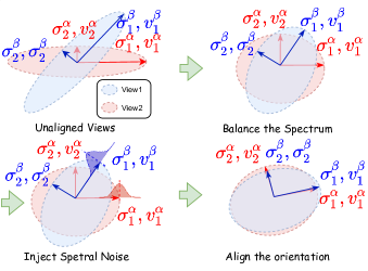
Figure 1: Our GCL with spectral feature augmentation by the incomplete power iteration implicitly performs three steps. Let blue and red ellipses represent spectra of feature maps $\mathbf{H}^{\alpha}$ and $\mathbf{H}^{\beta}$ of two views. Singular values of unaligned views (top left) are firstly rebalanced (top right) and the noise is injected into singular values (bottom left). Given rebalanced singular values, corresponding singular vectors are aligned with equalized emphasis (leading unbalanced singular values would emphasize the alignment of leading singular vectors, sacrificing the quality of alignment of other singular vectors).

Semi-supervised and supervised Graph Neural Networks (GNNs) (Velickovic et al. 2018; Hamilton, Ying, and Leskovec 2017; Song, Zhang, and King 2022; Zhang et al. 2022b) require full access to class labels. However, unsupervised GNNs (Klicpera, Bojchevski, and Günnemann 2019; Wu et al. 2019; Zhu and Koniusz 2021) and recent Self-Supervised Learning (SSL) models do not require labels (Song et al. 2021; Pan et al. 2018) to train embeddings. Among SSL methods, Contrastive Learning (CL) achieves comparable performance with its supervised counterparts on many tasks (Chen et al. 2020; Gao, Yao, and Chen 2021). CL has also been applied recently to the graph domain. A typical Graph Contrastive Learning (GCL) method forms multiple graph views via stochastic augmentation of the input to learn representations by contrasting so-called positive samples with negative samples (Zhu et al. 2020; Peng et al. 2020; Zhu, Sun, and Koniusz 2021; Zhu and Koniusz 2022; Zhang et al. 2022c). As an indispensable part of GCL, the significance of graph augmentation has been well studied (Hafidi et al. 2020; Zhu et al. 2021b; Yin et al. 2021). Popular random data augmentations are just one strategy to construct views, and their noise may affect adversely downstream tasks (Suresh et al. 2021; Tian et al. 2020). Thus, some works  (Yin et al. 2021; Tian et al. 2020; Suresh et al. 2021) learn graph augmentations but they require supervision.

The above issue motivates us to propose a simple/efficient data augmentation model which is complementary with existing augmentation strategies. We target Feature Augmentation (FA) as scarcely any FA works exist in the context of CL and GCL. In the image domain, a simple FA (Upchurch et al. 2017; Bengio et al. 2013) showed that perturbing feature representations of an image results in a representation of another image where both images share some semantics (Wang et al. 2019). However, perturbing features randomly ignores covariance of feature representations, and ignores semantics correlations. Hence, we opt for injecting random noise into the singular values of feature maps as such a spectral feature augmentation does not alter the orthogonal bases of feature maps by much, thus helping preserve semantics correlations.

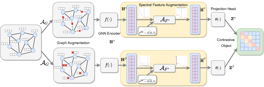
(a) Our pipeline.

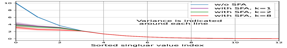
(b) Simulation: spectrum obtained by Alg. 1.

Figure 2: Our GCL model. Two graph views are generated by data augmentation and passed into graph neural network encoders with shared parameters to learn node representations. The proposed spectral feature augmentation rebalances (partially equalizes) the spectrum of each feature map, and implicitly injects the noise into rebalanced singular values. Such representations are fed into the projection head and the contrastive loss. Figure 1 explains the role of our spectral feature augmentation.

Moreover, as typical GCL aligns two data views (Wang and Isola 2020), unbalanced singular values of two data views may affect the quality of alignment. As several leading singular values (acting as weights on the loss) dominate the alignment process, GCL favors aligning the leading singular vectors of two data views while sacrificing remaining orthogonal directions with small singular values. In other words, the unbalanced spectrum leads to a suboptimal orthonormal bases alignment, which results in a suboptimal GCL model.

To address rebalancing of unbalanced spectrum and augmenting leading singular values, we present a novel and efficient Spectral Feature Augmentation (SFA). To this end, we propose the so-called incomplete power iteration which, under just one or two iterations, partially balances singular values of feature maps and implicitly injects the noise into these singular values. We evaluate our method on various datasets for node level tasks (i.e., node classification and node clustering). We also show that our method is compatible with other augmentation strategies and contrastive losses.

We summarize our contributions as follows:

1. We propose a simple/efficient spectral feature augmentation for GCL which is independent of different contrastive losses, i.e., we employ InfoNCE and Barlow Twin.

2. We introduce the so-called incomplete power iteration which, under just one or two iterations, partially balances spectra of two data views and injects the augmentation noise into their singular values. The rebalanced spectra help align orthonormal bases of both data views.

3. As the incomplete power iteration is stochastic in its nature, we derive its analytical form which provably demonstrates its spectrum rebalancing effect in expectation, and captures the variance of the spectral augmentation.

4. For completeness, we devise other spectral augmentation models, based on the so-called MaxExp and Power Norm. operators and Grassman feature maps, whose rebalancing and noise injection profiles differ with our method.

2 Related Work

Data Augmentation. Augmentations are usually performed in the input space. In computer vision, image transformations, i.e., rotation, flipping, color jitters, translation, noise injection (Shorten and Khoshgoftaar 2019), cutout and random erasure (DeVries and Taylor 2017) are popular. In neural language processing, token-level random augmentations, e.g., synonym replacement, word swapping, word insertion, and deletion (Wei and Zou 2019) are used. In transportation, conditional augmentation of road junctions is used (Prabowo et al. 2019). In the graph domain, attribute masking, edge permutation, and node dropout are popular (You et al. 2020a). Sun et al. (Sun, Koniusz, and Wang 2019) use adversarial graph perturbations. Zhu et al. (Zhu et al. 2021b) use adaptive graph augmentations based on the node/PageRank centrality (Page et al. 1999) to mask edges with varying probability.

Feature Augmentation. Samples can be augmented in the feature space instead of the input space (Feng et al. 2021). Wang et al. (Wang et al. 2019) augment the hidden space features, resulting in auxiliary samples with the same class identity but different semantics. A so-called channel augmentation perturbs the channels of feature maps (Wang et al. 2019) while GCL approach, COSTA (Zhang et al. 2022c), augments features via random projections. Some few-shot learning approaches augment features (Zhang et al. 2022a) while others estimate the “analogy” transformations between samples of known classes to apply them on samples of novel classes (Hariharan and Girshick 2017; Schwartz et al. 2018) or mix foregrounds and backgrounds (Zhang, Zhang, and Koniusz 2019). However, “analogy” augmentations are not applicable to contrastive learning due to the lack of labels.

Graph Contrastive Learning. CL is popular in computer vision, NLP (He et al. 2020; Chen et al. 2020; Gao, Yao, and Chen 2021), and graph learning. In the vision domain, views are formed by augmentations at the pixel level, whereas in the graph domain, data augmentation may act on node attributes or the graph edges. GCL often explores node-node, node-graph, and graph-graph relations for contrastive loss which is similar to contrastive losses in computer vision. Inspired by SimCLR (Chen et al. 2020), GRACE (Zhu et al. 2020) correlates graph views by pushing closer representations of the same node in different views and separating representations of different nodes, and Barlow Twin (Zbontar et al. 2021) avoids the so-called dimensional collapse  (Jing et al. 2021).

In contrast, we study spectral feature augmentations to perturb/rebalance singular values of both views. We outperform feature augmentations such as COSTA (Zhang et al. 2022c).

3 Proposed Method

Inspired by recent advances in augmentation-based GCL, our approach learns node representations by rebalancing spectrum of two data views and performing the spectral feature augmentation via the incomplete power iteration. SFA is complementary to the existing data augmentation approaches. Figure 2(a) illustrates our framework. The Notations section (supplementary material) explains our notations.

Graph Augmentation ($\mathcal{A}_{G}$). Augmented graph $(\tilde{\mathbf{A}},\tilde{\mathbf{X}})$ is generated by $\mathcal{A}_{G}$ by directly adding random perturbations to the original graph $({\mathbf{A}},{\mathbf{X}})$. Different augmented graphs are constructed given one input $(\mathbf{A},\mathbf{X})$, yielding correlated views, i.e., $(\widetilde{\mathbf{A}}^{\alpha},\widetilde{\mathbf{X}}^{\alpha})$ and $(\widetilde{\mathbf{A}}^{\beta},\widetilde{\mathbf{X}}^{\beta})$. In the common GCL setting (Zhu et al. 2020), the graph structure is augmented by permuting edges, whereas attributes by masking.

Graph Neural Network Encoders. Our framework admits various choices of the graph encoder. We opt for simplicity and adopt the commonly used graph convolution network (GCN) (Kipf and Welling 2017) as our base graph encoder. As shown in Fig. 2(a), we use a shared graph encoder for each view, i.e., $f:\mathbb{R}^{n\times d_{x}}\times\mathbb{R}^{n\times n}\longmapsto\mathbb{R}^{n\times d_{h}}$. We consider two graphs generated from $\mathcal{A}_{G}$ as two congruent structural views and define the GCN encoder with 2 layers as:

$$f(\mathbf{X},\mathbf{A})=\mathrm{GCN}_{2}\left(\mathrm{GCN}_{1}(\mathbf{X},\mathbf{A}),\mathbf{A}\right),$$ (1)

$$\quad\text{ where }\quad\mathrm{GCN}_{l}(\mathbf{X},\mathbf{A})=\sigma\big{(}\hat{\mathbf{D}}^{-\frac{1}{2}}\hat{\mathbf{A}}\hat{\mathbf{D}}^{-\frac{1}{2}}\mathbf{X}\Theta\big{)}.$$

Moreover, $\tilde{\mathbf{A}}=\hat{\mathbf{D}}^{-1/2}\hat{\mathbf{A}}\hat{\mathbf{D}}^{-1/2}\in\mathbb{R}^{n\times n}$ is the degree-normalized adjacency matrix, $\hat{\mathbf{D}}\in\mathbb{R}^{n\times n}$ is the degree matrix of $\hat{\mathbf{A}}=\mathbf{A}+\mathbf{I}_{\mathbf{N}}$ where $\mathbf{I}_{\mathbf{N}}$ is the identity matrix, $\mathbf{X}\in\mathbb{R}^{n\times d_{x}}$ contains the initial node features, $\bm{\Theta}\in\mathbb{R}^{d_{x}\times d_{h}}$ contains network parameters, and $\sigma(\cdot)$ is a parametric ReLU (PReLU). The encoder outputs feature maps $\mathbf{H}^{\alpha}$ and $\mathbf{H}^{\beta}$ for two views.

Spectral Feature Augmentation (SFA). $\mathbf{H}^{\alpha}$ and $\mathbf{H}^{\beta}$ are fed to the feature augmenting function $\mathcal{A}_{F^{*}}$ where random noises are added to the spectrum via the incomplete power iteration. We explain the proposed SFA in the Spectral Feature Augmentation for GCL section and detail its properties in Propositions 1, 2 and 3. SFA results in the spectrally-augmented feature maps, i.e., $\widetilde{\mathbf{H}}^{\alpha}$ and $\widetilde{\mathbf{H}}^{\beta}$. SFA is followed by a shared projection head $\theta:\mathbb{R}^{n\times d_{h}}\longmapsto\mathbb{R}^{n\times d_{z}}$ which is an MLP with two hidden layers and PReLU nonlinearity. It maps $\widetilde{\mathbf{H}}^{\alpha}$ and $\widetilde{\mathbf{H}}^{\beta}$ into two node representations $\mathbf{Z}^{\alpha},\mathbf{Z}^{\beta}\in\mathbb{R}^{n\times d_{z}}$ (two congruent views of one graph) on which the contrastive loss is applied. As described in (Chen et al. 2020), it is beneficial to define the contrastive loss on $\mathbf{Z}$ rather than $\mathbf{H}$.

Contrastive Training. To train the encoders end-to-end and learn rich node representations that are agnostic to downstream tasks, we utilize the InfoNCE loss (Chen et al. 2020):

$$\mathcal{L}_{contrastive}(\tau)=\underbrace{\underset{\mathbf{z},\mathbf{z}^{+}}{\mathbb{E}}\left[-\mathbf{z}^{\top}\mathbf{z}^{+}/\tau\right]}_{alignment}$$ (2)

$$+\underbrace{\underset{\mathbf{z},\mathbf{z}^{+}}{\mathbb{E}}\Big{[}\log\Big{(}e^{{\mathbf{z}^{\top}\mathbf{z}^{+}}/{\tau}}\;\;+\!\!\!\!\!\!\!\!\sum_{\mathbf{z}^{-}\in\mathbf{Z}^{\alpha\beta}\setminus\{\mathbf{z},\ \mathbf{z}^{+}\}}\!\!\!\!\!\!\!\!e^{{\mathbf{z}^{\top}\mathbf{z}^{-}}/{\tau}}\Big{)}\Big{]}}_{uniformity},$$

where $\mathbf{z}$ is the representation of the anchor node in one view (i.e., $\mathbf{z}\in\mathbf{Z}^{\alpha}$) and $\mathbf{z}^{+}$ denotes the representation of the anchor node in another view (i.e., $\mathbf{z}^{+}\in\mathbf{Z}^{\beta}$), whereas $\{\mathbf{z}^{-}\}$ are from the set of node representations other than $\mathbf{z}$ and $\mathbf{z}^{+}$ (i.e., $\mathbf{Z}^{\alpha\beta}\!\equiv\mathbf{Z}^{\alpha}\cup\mathbf{Z}^{\beta}$ and $\mathbf{z}^{-}\!\in\mathbf{Z}^{\alpha\beta}\setminus\{\mathbf{z},\ \mathbf{z}^{+}\}$). The first part of Eq. (2) maximizes the alignment of two views (representations of the same node become similar). The second part of Eq. (2) minimizes the pairwise similarity via LogSumExp. Pushing node representations away from each other makes them uniformly distributed (Wang and Isola 2020).

Algorithm 1 Spectral Feature Augmentation ($\mathcal{A}_{F^{*}}$)

Input: feature map $\mathbf{H}$; the number of iterations $k$;

$\mathbf{r}^{(0)}\sim\mathcal{N}(0,\mathbf{I})$

for $i=1$ to $k$ do

   $\mathbf{r}^{(i)}=\mathbf{H}^{\top}\mathbf{H}\mathbf{r}^{(i-1)}$

end for

$\widetilde{\mathbf{H}}=\mathbf{H}-\frac{\mathbf{H}\mathbf{r}^{(k)}{\mathbf{r}^{(k)}}^{\top}}{\|\mathbf{r}^{(k)}\|_{2}^{2}}$

Return $\widetilde{\mathbf{H}}$

3.1 Spectral Feature Augmentation for GCL

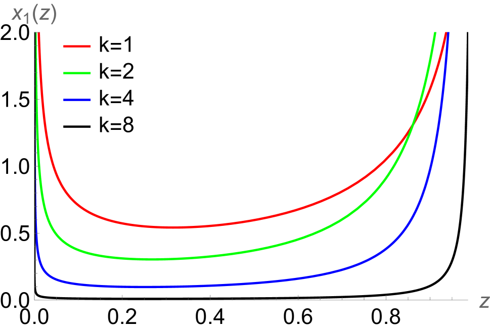
(a)

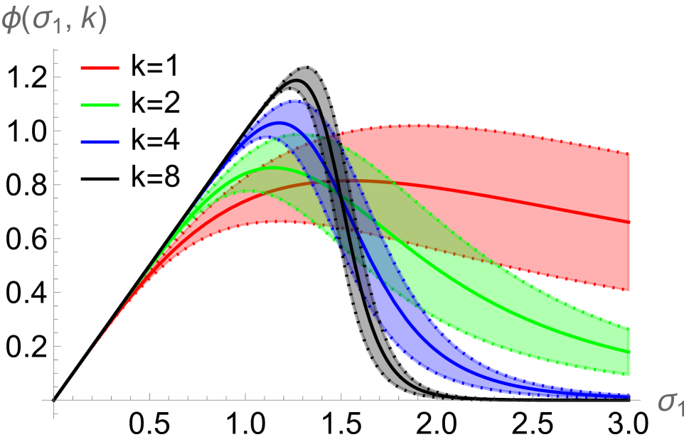
(b)

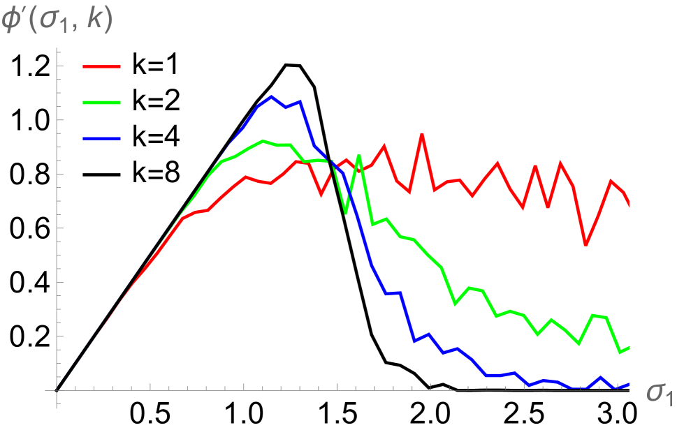
(c)

Figure 3: Toy illustration of Prop. 2 and 3. Let $\sigma_{2},\cdots,\sigma_{5}$ be $1.5,0.9,0.2,0.01$. We investigate the impact of iterations $k\in\{1,2,4,8\}$. Fig. 3(a) shows distribution $x(z)$ given $\sigma_{1}=2$. Fig. 3(b) shows the expected value $\phi(\sigma_{1},k)=\sigma_{1}(1-\lambda_{1})$ where $\lambda_{1}=\mathbb{E}_{z\sim x_{1}}(z)$ for $0\leq\sigma_{1}\leq 3$. The deviation is indicated by $\phi_{\pm\omega_{1}}(\sigma_{1},k)=\sigma_{1}(1-\lambda_{1}\pm\omega_{1})$. Finally, Fig. 3(c) is obtained via Alg. 1 (the incomplete power iteration). To this end, we generated randomly a feature matrix $\mathbf{H}$ and substituted its singular values by $\sigma_{1},\cdots,\sigma_{5}$. Notice that for $k=1$, $1\leq\sigma_{1}\leq 3$, push-forward $\phi(\sigma_{1},1)$ and $\phi^{\prime}(\sigma_{1},1)$ in Fig. 3(b) and 3(c) are around 0.8 (the balancing of spectrum) and the high deviation indicates the singular value undergoes the spectral augmentation. For $k\geq 2$, both balancing and spectral augmentation effects decline. Note theoretical $\phi$ in Prop. 2 and real $\phi^{\prime}$ from Alg. 1 match.

Our spectral feature augmentation is inspired by the rank-1 update (Yu, Cai, and Li 2020). Let $\mathbf{H}=f(\mathbf{X},\mathbf{A})$ be the graph feature map with the singular decomposition $\mathbf{H}=\mathbf{U}\mathbf{\Sigma}\mathbf{V}^{\top}$ where $\mathbf{H}\in\mathbb{R}^{n\times d_{h}}$, $\mathbf{U}$ and $\mathbf{V}$ are unitary matrices, and $\mathbf{\Sigma}=\text{diag}(\sigma_{1},\sigma_{2},\cdots,\sigma_{d_{h}})$ is the diagonal matrix with singular values $\sigma_{1}\geq\sigma_{2}\geq\cdots\geq\sigma_{d_{h}}$. Starting from a random point $\mathbf{r}^{(0)}\sim\mathcal{N}(0,\mathbf{I})$ and function $\mathbf{r}^{(k)}=\mathbf{H}^{\top}\mathbf{H}\mathbf{r}^{(k-1)}$, we generate a set of augmented feature maps $\widetilde{\mathbf{H}}$ by:

$$\widetilde{\mathbf{H}}\big{(}\mathbf{H};\mathbf{r}^{(0)}\big{)}=\mathbf{H}-\mathbf{H}_{\text{LowRank}}=\mathbf{H}-\frac{\mathbf{H}\mathbf{r}^{(k)}\mathbf{r}^{(k)\top}}{\|\mathbf{r}^{(k)}\|_{2}^{2}}.$$ (3)

We often write $\widetilde{\mathbf{H}}$ rather than $\widetilde{\mathbf{H}}\big{(}\mathbf{H};\mathbf{r}^{(0)}\big{)}$, and we often think of $\widetilde{\mathbf{H}}$ as a matrix. We summarize the proposed SFA in Alg. 1.

Proposition 1.

Let $\widetilde{\mathbf{H}}$ be the augmented feature matrix obtained via Alg. 1 for the $k$-th iteration starting from a random vector $\mathbf{r}^{(0)}$ drawn from $\mathcal{N}(0,\mathbf{I})$. Then $\,\mathbb{E}_{\mathbf{r}^{(0)}\sim\mathcal{N}(0,\mathbf{I})}(\widetilde{\mathbf{H}}\big{(}\mathbf{H};\mathbf{r}^{(0)}\big{)})=\mathbf{U}\widetilde{\Sigma}\mathbf{V}^{\top}\!$ has rebalanced spectrum $\;\widetilde{\bm{\Sigma}}=\text{diag}\big{[}(1-\lambda_{1}(k)\sigma_{1},(1-\lambda_{2}(k))\sigma_{2},\cdots,(1-\lambda_{d_{h}}(k))\sigma_{d_{h}}\big{]}\;$ where $\lambda_{i}(k)=\mathbb{E}_{\mathbf{y}\sim\mathcal{N}(0;\mathbf{I})}\big{(}\frac{\left(y_{i}\sigma_{i}^{2k}\right)^{2}}{\sum_{l=1}^{d_{h}}\left(y_{l}\sigma_{l}^{2k}\right)^{2}})$ and $\mathbf{y}=\mathbf{V}^{\top}\mathbf{r}^{(0)}$, because $0\leq 1-\lambda_{1}(k)\leq 1-\lambda_{2}(k)\leq\cdots\leq 1-\lambda_{d_{h}}(k)\leq 1\;$ for $\;\sigma_{1}\geq\sigma_{2}\geq\cdots\geq\sigma_{d_{h}}$ (sorted singular values from the SVD), and so $(1-\lambda_{i})$ gets smaller or larger as $\sigma_{i}$ gets larger or smaller, respectively.

Proposition 2.

Analytical Expectation. Let $\beta_{i}=(\sigma_{i}^{2k})^{2}$, then the expected value $\mathbb{E}_{\mathbf{y}\sim\mathcal{N}(0;\mathbf{I})}\frac{\beta_{i}y_{i}^{2}}{\beta_{i}y_{i}^{2}+\sum_{l\neq i}\beta_{l}y^{2}_{l}}=\lambda_{i}(k)$ can be expressed as $\mathbb{E}(x_{i})$ over random variable $x_{i}\!=\!\frac{u}{u+v_{i}}$ for $u\!\sim\!\mathcal{G}(\frac{1}{2},2)$ and $v_{i}\!\sim\!\mathcal{G}(\alpha_{i},2\gamma_{i})$ ($\mathcal{G}$ is Gamma distr.) with $\alpha_{i}\!=\!\frac{1}{2}\frac{(\sum_{l\neq i}\beta_{l})^{2}}{\sum_{l\neq i}\beta_{l}^{2}}$ and $\gamma_{i}\!=\!\frac{1}{\beta_{i}}\frac{\sum_{l\neq i}\beta_{l}^{2}}{\sum_{l\neq i}\beta_{l}}$. As PDF $x^{\bullet}_{i}(z)\!=\!\frac{\gamma_{i}}{(1-(1-z)\gamma_{i})^{2}}\cdot\mathcal{B}\big{(}\frac{\gamma_{i}z}{1-(1-z)\gamma_{i}};\frac{1}{2},\alpha_{i}\big{)}$ where $\mathcal{B}$ is the Beta distribution and $x^{\bullet}_{i}(z)$ enjoys the support $z\in[0;1]$, then $\lambda_{i}=\mathbb{E}(z)=\int_{0}^{1}z\cdot x^{\bullet}_{i}(z)\,\mathrm{d}z=\gamma_{i}^{\frac{1}{2}}\frac{\Gamma(\frac{3}{2})\Gamma(\frac{1}{2}+\alpha_{i})}{\Gamma(\frac{1}{2})\Gamma(\frac{3}{2}+\alpha_{i})}\cdot{{}_{2}F_{1}}\big{(}\frac{3}{2},\frac{1}{2}\!+\!\alpha_{i},\frac{3}{2}\!+\!\alpha_{i},1\!-\!\gamma_{i}\big{)}$ where ${{}_{2}F_{1}}(\cdot)$ is the so-called Hypergeometric function.

Proof.

See Proof of Proposition 2 (supplementary material). ∎

Proposition 3.

Analytical Variance. Following assumptions of Proposition 2, the variance $\omega^{2}_{i}$ of $x^{\bullet}_{i}(z)$ can be expressed as $\omega^{2}_{i}=\mathbb{E}(z^{2})-(\mathbb{E}(z))^{2}=\int_{0}^{1}z^{2}\cdot x^{\bullet}_{i}(z)\,\mathrm{d}z-\lambda^{2}_{i}=$ $0.56419\,\gamma^{\frac{1}{2}}\frac{\Gamma(\frac{1}{2}+\alpha_{i})}{\Gamma(\alpha_{i})}\allowbreak\big{(}0.4\cdot{{}_{2}F_{1}}\big{(}\frac{5}{2},1\!-\!\alpha_{i},\frac{7}{2},1\big{)}\cdot\allowbreak{{}_{2}F_{1}}\big{(}\frac{5}{2},\frac{3}{2}\!+\!\alpha_{i},\frac{5}{2}\!+\!\alpha_{i},1\!-\!\gamma_{i}\big{)}+0.28571(\gamma_{i}-1)\cdot{{}_{2}F_{1}}\big{(}\frac{7}{2},1\!-\!\alpha_{i},\frac{9}{2},1\big{)}\cdot{{}_{2}F_{1}}\big{(}\frac{7}{2},\frac{3}{2}\!+\!\alpha_{i},\frac{7}{2}\!+\!\alpha_{i},1\!-\!\gamma_{i}\big{)}\big{)}-\lambda^{2}_{i}$.

Proof.

See Proof of Proposition 3 (supplementary material). ∎

3.2 Why does the Incomplete Power Iteration work?

Having discussed SFA, below we show how SFA improves the alignment/generalization by flattening large and boosting small singular values due to rebalanced spectrum.

Improved Alignment. SFA rebalances the weight penalty (by rebalancing singular values) on orthonormal bases, thus improving the alignment of two correlated views. Consider the alignment part of Eq. (2) and ignore the projection head $\theta$ for brevity. The contrastive loss (temperature $\tau>0$, $n$ nodes) on $\mathbf{H}^{\alpha}$ and $\mathbf{H}^{\beta}$ maximizes the alignment of two views:

$$\!\begin{aligned} \mathcal{L}_{a}&=\underset{\mathbf{h}^{\alpha},\mathbf{h}^{\beta}}{\mathbb{E}}(\mathbf{h}^{\alpha\top}\mathbf{h}^{\beta}/\tau)=\frac{1}{n\tau}\text{Tr}(\mathbf{H}^{\alpha\top}\mathbf{H}^{\beta})\\[-5.0pt] &=\frac{1}{n\tau}\sum_{i=1}^{d_{h}}({\sigma}^{\alpha}_{i}{\mathbf{v}}_{i}^{\alpha\top}\!{\mathbf{v}}^{\beta}_{i})({\sigma}^{\beta}_{i}{{\mathbf{u}}}^{\alpha\top}_{i}\!{\mathbf{u}}^{\beta}_{i}).\end{aligned}\vspace{-0.2cm}$$ (5)

The above equation indicates that for $\sigma^{\alpha}_{i}\geq 0$ and $\sigma^{\beta}_{i}\geq 0$, the maximum is reached if the right and left singular value matrices are perfectly aligned, i.e., $\mathbf{U}^{\alpha}\!=\!\mathbf{U}^{\beta}$ and $\mathbf{V}^{\alpha}\!=\!\mathbf{V}^{\beta}$. Notice the singular values $\sigma^{\alpha}_{i}$ and $\sigma^{\alpha}_{i}$ serve as weighs for the alignment of singular vectors. As the singular value gap $\Delta\sigma_{12}=\sigma_{1}-\sigma_{2}$ is usually significant (spectrum of feature maps usually adheres to the power law $ai^{-\kappa}$ ($i$ is the index of sorted singular values, $a$ and $\kappa$ control the magnitude/shape), the large singular values tend to dominate the optimization. Such an issue makes Eq. (5) focus only on aligning the direction of dominant singular vectors, while neglecting remaining singular vectors, leading to a poor alignment of the orthonormal bases. In contrast, SFA alleviates this issue. According to Prop. 1, Eq. (5) with SFA becomes:

$$\!\!\!\begin{aligned} \mathcal{L}^{*}_{a}&=\underset{\mathbf{h^{\alpha}},\mathbf{h^{\beta}}/\tau}{\mathbb{E}}\underset{\mathbf{r}^{\alpha},\mathbf{r^{\beta}\sim\mathcal{N}(0,\mathbf{I})}}{\mathbb{E}}(\tilde{\mathbf{h}}^{\alpha\top}\tilde{\mathbf{h}}^{\beta})\\[-4.0pt] &=\frac{1}{n\tau}\sum_{i=1}^{d_{h}}(1\!-\!\lambda_{i}^{\alpha}){\sigma}^{\alpha}_{i}({\mathbf{v}}_{i}^{\alpha\top}{\mathbf{v}}^{\beta}_{i})(1\!-\!\lambda_{i}^{\beta}){\sigma}^{\beta}_{i}({{\mathbf{u}}}^{\alpha\top}_{i}{\mathbf{u}}^{\beta}_{i}).\end{aligned}\!$$ (6)

Improved Alignment Yields Better Generalization Bound. To show SFA achieves the improved generalization bound we quote the following theorem (Huang, Yi, and Zhao 2021).

Theorem 1.

Given a Nearest Neighbour classifier $G_{f}$, the downstream error rate of $G_{f}$ is $\operatorname{Err}\left(G_{f}\right)\!\leq\!(1\!-\!\sigma)\!+\!R_{\varepsilon},$ where $R_{\varepsilon}\!\!=\!\!P_{\mathbf{x}_{1},\mathbf{x}_{2}\in\mathcal{A}(\mathbf{x})}\{\|f\left(\mathbf{x}_{1}\right)\!-\!f\left(\mathbf{x}_{2})\|\!\geq\!\varepsilon\right\}\!\leq\!\frac{\sqrt{2-2\mathcal{L}_{a}}}{\varepsilon}$, $\sigma$ is the parameter of the so-called $(\sigma,\delta)$-augmentation (for each latent class, the proportion of samples located in a ball with diameter $\delta$ is larger than $\sigma$, $\mathcal{A}(\cdot)$ is the set of augmented samples, $f(\cdot)$ is the encoder, and $\{\|\cdot\|\!\geq\!\varepsilon\}$ is the set of samples with $\varepsilon$-close representations among augmented data.

Proof.

See Proof of Theorem 1 (supp. material). ∎

Theorem 1 says the key to better generalization of contrastive learning is better alignment $\|f(\mathbf{x}_{1})-f(\mathbf{x}_{2})\|$ of positive samples. SFA improves alignment by design. See Why does the Incomplete Power Iteration work?   See empirical result in the Analysis on Spectral Feature Augmentation section. Good alignment (e.g., Fig. 7) due to spectrum rebalancing (e.g., Fig. 7) enjoys $\mathcal{L}_{a}\leq\mathcal{L}^{*}_{a}$ (Eq. (5) and (6)) so one gets $\!R_{\varepsilon}^{*}\!\leq\!R_{\varepsilon}$ and the lower generalization bound $\operatorname{Err}\big{(}G^{*}_{f}\big{)}\leq\operatorname{Err}\big{(}G_{f}\big{)}$. Asterisk ^∗ means SFA is used ($\mathcal{L}^{*}_{a}$ replaces $\mathcal{L}_{a}$).

4 Experiments

Method	WikiCS	Am-Comput.	Am-Photo	Cora	CiteSeer	PubMed
RAW fatures	$71.98\pm 0.00$	$73.81\pm 0.00$	$78.53\pm 0.00$	$64.61\pm 0.22$	$65.77\pm 0.15$	$82.02\pm 0.26$
DeepWalk	$74.35\pm 0.06$	$85.68\pm 0.06$	$89.44\pm 0.11$	$74.61\pm 0.22$	$50.77\pm 0.15$	$80.11\pm 0.25$
DGI	$75.35\pm 0.14$	$83.95\pm 0.47$	$91.61\pm 0.22$	$82.15\pm 0.63$	$69.51\pm 0.52$	$86.01\pm 0.26$
MVGRL	$77.52\pm 0.08$	$87.52\pm 0.11$	$91.74\pm 0.07$	$83.11\pm 0.12$	$73.33\pm 0.03$	$84.27\pm 0.04$
GRACE	$78.19\pm 0.48$	$87.25\pm 0.25$	$92.15\pm 0.25$	$83.51\pm 0.25$	$73.63\pm 0.20$	$85.51\pm 0.37$
GCA	$78.35\pm 0.05$	$87.85\pm 0.31$	$92.49\pm 0.16$	$82.89\pm 0.21$	$72.89\pm 0.13$	$85.12\pm 0.23$
SUGRL	$77.72\pm 0.28$	$88.83\pm 0.23$	$93.28\pm 0.42$	$83.47\pm 0.55$	$73.08\pm 0.45$	$84.91\pm 0.31$
MERIT	$77.92\pm 0.43$	$87.53\pm 0.26$	$93.12\pm 0.42$	$84.11\pm 0.65$	$74.34\pm 0.43$	$84.12\pm 0.23$
BGRL	$79.11\pm 0.62$	$87.37\pm 0.40$	$91.57\pm 0.44$	$83.77\pm 0.57$	$73.07\pm 0.06$	$84.62\pm 0.35$
G-BT	$76.85\pm 0.62$	$86.86\pm 0.33$	$92.63\pm 0.57$	$83.63\pm 0.44$	$72.95\pm 0.17$	$84.52\pm 0.12$
COSTA	$79.12\pm 0.02$	$88.32\pm 0.03$	$92.56\pm 0.45$	$84.32\pm 0.22$	$72.92\pm 0.31$	$86.01\pm 0.22$
SFA${}_{\text{BT}}$	${\color[rgb]{0,0,1}\mathbf{80.22}\pm 0.05}$	${\color[rgb]{0,0,1}88.14\pm 0.15}$	${\color[rgb]{0,0,1}92.83\pm 0.14}$	${\color[rgb]{0,0,1}84.10\pm 0.01}$	${\color[rgb]{0,0,1}73.73\pm 0.03}$	${\color[rgb]{0,0,1}85.63\pm 0.07}$
SFA${}_{\text{InfoNCE}}$	${\color[rgb]{0,0,1}79.98\pm 0.05}$	${\color[rgb]{0,0,1}\mathbf{89.24\pm 0.27}}$	${\color[rgb]{0,0,1}\mathbf{93.53\pm 0.16}}$	${\color[rgb]{0,0,1}\mathbf{85.89\pm 0.01}}$	${\color[rgb]{0,0,1}\mathbf{75.31\pm 0.03}}$	${\color[rgb]{0,0,1}\mathbf{86.29\pm 0.13}}$

Table 1: Node classification on graph datasets. Note that SFA${}_{\text{InfoNEC}}$ and SFA${}_{\text{BT}}$ can be directly compared to GRACE and G-BT. (Accuracy is reported.)

Figure 4: Running time per epoch in seconds.

Datasets	w/o SFA	SFA
		$k=1$
Cora	$165$	$172$
CiteSeer	$164$	$173$
WikiCS	$1334$	$1343$

Table 2: Running time per epoch in seconds.

Method	SFA (ours)	SVD	Random SVD
Time	0.25 hour	12 hours	1.2 hours

Table 3: Running time on Ogb-arxiv.

Ogb-arxiv	Validation	Test
MLP	$57.6\pm 0.2$	$55.5\pm 0.3$
Node2vec	$71.2\pm 0.3$	$70.0\pm 0.3$
MVGLR	$69.3\pm 0.3$	$68.2\pm 0.2$
DGI	$71.2\pm 0.1$	$70.3\pm 0.1$
SUGRL	$70.2\pm 0.1$	$69.3\pm 0.2$
MERIT	$67.2\pm 0.1$	$65.3\pm 0.2$
GRACE	$71.4\pm 0.5$	$70.8\pm 0.1$
G-BT	$71.1\pm 0.3$	$70.0\pm 0.2$
COSTA	$71.6\pm 0.4$	$71.0\pm 0.4$
SFA${}_{\text{Info}}$	$\bf 72.3\pm 0.1$	$\bf 71.6\pm 0.4$

Table 4: Node classification.

Method	CIFAR10	CIFAR100	ImageNet-100
SimCLR	$90.5$	$65.5$	$76.8$
SFA${}_{\text{SimCLR}}$	$\mathbf{91.6}$	$\mathbf{66.7}$	${\color[rgb]{0,0,1}\mathbf{77.7}}$
BalowTw	$92.0$	$69.7$	$80.0$
SFA${}_{\text{BT}}$	$\mathbf{92.5}$	$\mathbf{70.4}$	$\mathbf{80.9}$
Siamese	$90.51$	$66.04$	$74.5$
SFA${}_{\text{Siamese}}$	$\mathbf{91.23}$	66.99	$\mathbf{75.6}$
SwAV	$89.17$	$64.88$	$74.0$
SFA${}_{\text{SwAV}}$	$\mathbf{90.12}$	$\mathbf{65.82}$	$\mathbf{74.8}$

Table 5: Image classification on CIFAR10, CIFAR100 and ImageNet-100.

Method	NCI1	PROTEIN	DD
GraphCL	$77.8\pm 0.4$	$74.3\pm 0.4$	${77.8\pm 0.4}$
LP-Info	$75.8\pm 1.2$	${\color[rgb]{0,0,1}74.6\pm 0.2}$	$72.5\pm 1.9$
JOAO	${\color[rgb]{0,0,1}78.0\pm 0.4}$	${74.5\pm 0.4}$	${\color[rgb]{0,0,1}77.5\pm 0.5}$
SimGRACE	$77.4\pm 1.0$	$73.9\pm 0.1$	$77.3\pm 1.1$
SFA${}_{\text{InfoNEC}}$	${\color[rgb]{0,0,1}\mathbf{78.7\pm 0.4}}$	${\color[rgb]{0,0,1}\mathbf{75.4\pm 0.4}}$	${\color[rgb]{0,0,1}\mathbf{78.6\pm 0.4}}$

Table 6: Graph classification. (SFA${}_{\text{InfoNEC}}$ can be directly compared with GraphCL.)

$\mathcal{A}_{G}$	$\mathcal{A}_{F}$	$\mathcal{A}_{F^{*}}$	Am-Comput.	Cora	CiteSeer
$\times$	$\times$	$\times$	$85.01$	$80.04$	$71.35$
$\checkmark$	$\times$	$\times$	$87.25$	$82.23$	$74.56$
$\times$	$\times$	$\checkmark$	$86.74$	$84.19$	$73.15$
$\checkmark$	$\times$	$\checkmark$	${\color[rgb]{0,0,1}\mathbf{88.74}}$	${\color[rgb]{0,0,1}\mathbf{85.90}}$	${\color[rgb]{0,0,1}\mathbf{75.05}}$
$\checkmark$	$\checkmark$	$\times$	$87.55$	$83.35$	$74.45$
$\checkmark$	$\checkmark$	$\checkmark$	${\color[rgb]{0,0,1}{88.69}}$	${\color[rgb]{0,0,1}{84.50}}$	${\color[rgb]{0,0,1}{74.70}}$

Table 7: Ablation study on different augmentation strategies: $\mathcal{A}_{G}$, $\mathcal{A}_{F}$ and $\mathcal{A}_{F^{*}}$.

Below we conduct experiments on the node classification, node clustering, graph classification and image classification. For fair comparisons, we use the same experimental setup as the representative Graph SSL (GSSL) methods (i.e., GCA (Zhu et al. 2020) and GRACE (Zhu et al. 2021b)).

Datasets. We use five popular datasets (Zhu et al. 2020, 2021b; Velickovic et al. 2019), including citation networks (Cora, CiteSeer) and social networks (Wiki-CS, Amazon-Computers, Amazon-Photo) (Kipf and Welling 2017; Sinha et al. 2015; McAuley et al. 2015; Mernyei and Cangea 2020). For graph classification, we use NCI1, PROTEIN and DD (Dobson and Doig 2003; Riesen and Bunke 2008). For image classification we use CIFAR10/100 (Krizhevsky, Hinton et al. 2009) and ImageNet-100 (Deng et al. 2009). See the Baseline Setting section for details (supplementary material).

Baselines. We focus on three groups of SSL models. The first group includes traditional GSSL, i.e., Deepwalk (Perozzi, Al-Rfou, and Skiena 2014), node2vec (Grover and Leskovec 2016), and GAE (Kipf and Welling 2016). The second group is contrastive-based GSSL, i.e., Deep Graph Infomax (DGI) (Velickovic et al. 2019), Multi-View Graph Representation Learning (MVGRL) (Hassani and Ahmadi 2020), GRACE (Zhu et al. 2020), GCA (Zhu et al. 2021b),  (Jin et al. 2021) SUGRL (Mo et al. 2022). The last group does not require explicit negative samples, i.e., Graph Barlow Twins(G-BT) (Bielak, Kajdanowicz, and Chawla 2021) and BGRL (Thakoor et al. 2021). We also compare SFA with COSTA (Zhang et al. 2022c) (GCL with feat. augmentation).

Evaluation Protocol. We adopt the evaluation from (Velickovic et al. 2019; Zhu et al. 2020, 2021b). Each model is trained in an unsupervised manner on the whole graph with node features. Then, we pass the raw features into the trained encoder to obtain embeddings and train an $\ell_{2}$-regularized logistic regression classifier. Graph Datasets are randomly divided into 10%, 10%, 80% for training, validation, and testing. We report the accuracy with mean/standard deviation over 20 random data splits.

Implementation details We use Xavier initialization for the GNN parameters and train the model with Adam optimizer. For node/graph classification, we use 2 GCN layers. The logistic regression classifier is trained with $5,000$ (guaranteed converge). We also use early stopping with a patience of 20 to avoid overfitting. We set the size of the hidden dimension of nodes to from ${128}$ to $512$. In clustering, we train a k-means clustering model. For the chosen hyper-parameters see Section D.2. We implement the major baselines using PyGCL (Zhu et al. 2021a). The detailed settings of augmentation and contrastive objectives are in Table 12 of Section D.3.

4.1 Main Results

Node Classification. We employ node classification as a downstream task to showcase SFA. The default contrastive objective is InfoNCE or the BT loss. Table 7 shows that SFA consistently achieves the best results on all datasets. Notice that the graph-augmented GSSL methods, including GSSL with SFA, significantly outperform the traditional methods, illustrating the importance of data augmentation in GSSL. Moreover, we find that the performance of GCL methods (i.e., GRACE, GCA, DGI, MVGRL) improves by a large margin when integrating with SFA (e.g., major baseline, GRACE, yields 3% and 4% gain on Cora and Citeseer), which shows that SFA is complementary to graph augmentations. SFA also works with the BT loss and improves its performance.

Graph Classification. By adopting the graph-level GNN encoder, SFA can be used for the graph-level pre-taining. Thus, we compare SFA with graph augmentation-based models (i.e., GarphCL (You et al. 2020b), JOAO (You et al. 2021)) and augmentation-free models (i.e., SimGrace (Xia et al. 2022), LP-Info (You et al. 2022)). Table 7 shows that SFA outperforms all baselines on the three datasets.

Image Classification. As SFA perturbs the spectrum of feature maps, it is also applicable to the image domain. Table 7 presents the top-1 accuracy on CIFAR10/100 and ImageNet-100. See also the Implementation Details (supp. material).

Runtimes. Table 2 and Fig. 4 show SFA incurs a negligible runtime overhead (few matrix-matrix(vector) multiplications). The cost of SFA for $k\!<\!8$ iterations is negligible.

To rebalance the spectrum, choices for a push-forward function whose curve gets flatter as singular values get larger are many but they require SVD to rebalance singular values directly. The complexity of SVD is $\mathcal{O}(nd_{h}^{2})$ for $n\!\gg\!d_{h}$, which is costly in GCL as SVD has to be computed per mini-batch (and SVD is unstable in back-prop. due to non-simple singular values ). Table 3 shows the runntime on Ogb-arixv.

4.2 Analysis on Spectral Feature Augmentation

Improved Alignment. We show that SFA improves the alignment of two views during training. Let $\mathbf{H}^{\alpha}$ and $\mathbf{H}^{\beta}$ ($\widetilde{\mathbf{H}}^{\alpha}$ and $\widetilde{\mathbf{H}}^{\beta}$) denote the feature maps of two views without (with) applying SFA. The alignment is computed by $\|\mathbf{H}^{\alpha}-\mathbf{H}^{\beta}\|^{2}_{F}$ (or $\|\tilde{\mathbf{H}}^{\alpha}-\tilde{\mathbf{H}}^{\beta}\|^{2}_{F}$). Fig. 7 shows that SFA achieves better alignment. See also the Additional Empirical Results.

Empirical Evolution of Spectrum. Fig. 7 (Cora) shows how the singular values of features maps ${\mathbf{H}}$ (without SFA) and $\tilde{\mathbf{H}}$ (with SFA) evolve. As training progresses, the gap between consecutive singular values gradually decreases due to SFA. The leading components of spectrum (where the signal is) become more balanced: empirical results match Prop. 1 & 2.

Ablations on Augmentations. Below, we compare graph augmentation $\mathcal{A}_{G}$, channel feature augmentation $\mathcal{A}_{F}$ (random noise added to embeddings directly) and the spectral feature augmentation $\mathcal{A}_{F^{*}}$. Table 7 shows that using $\mathcal{A}_{G}$ or $\mathcal{A}_{F^{*}}$ alone improves performance. For example, $\mathcal{A}_{G}$ yields 2.2%, 2.2% and 3.2% gain on Am-Computer, Cora, and CiteSeer. $\mathcal{A}_{F^{*}}$ yields 1.7%, 4.1% and 1.8% gain on Am-Computer, Cora, and CiteSeer. Importantly, when both $\mathcal{A}_{G}$ and $\mathcal{A}_{F^{*}}$ are applied, the gain is 3.7%, 6.0% and 4.8% on Am-Computer, Cora, and CiteSeer over “no augmentations”. Thus, SFA is complementary to existing graph augmentations. We also notice that $\mathcal{A}_{F^{*}}$ with $\mathcal{A}_{G}$ outperforms $\mathcal{A}_{F}$ with $\mathcal{A}_{G}$ by 1.1%, 2.4% and 1.7%, which highlights the benefit of SFA.

Effect of Number of Iterations ($k$). Below, we analyze how $k$ in Eq. (3) influences the performance. We set $k\in\{0,1,2,4,8\}$ in our model with the InfoNCE loss on Cora, Citeseer and Am-Computer. The case of $k=0$ means that no power iteration is used, i.e., the solution simplifies to the feature augmentation by subtracting from $\mathbf{H}$ perturbation $\mathbf{H}\mathbf{r}^{(0)}{\mathbf{r}^{(0)}}^{\top}\!\!/\|\mathbf{r}^{(0)}\|_{2}^{2}$ with random $\mathbf{r}^{(0)}$. Table 8 shows that without power iteration, the performance of the model drops , i.e., 1.5%, 3.3% and 2.2% on Am-Comp., Cora and Citeseer.

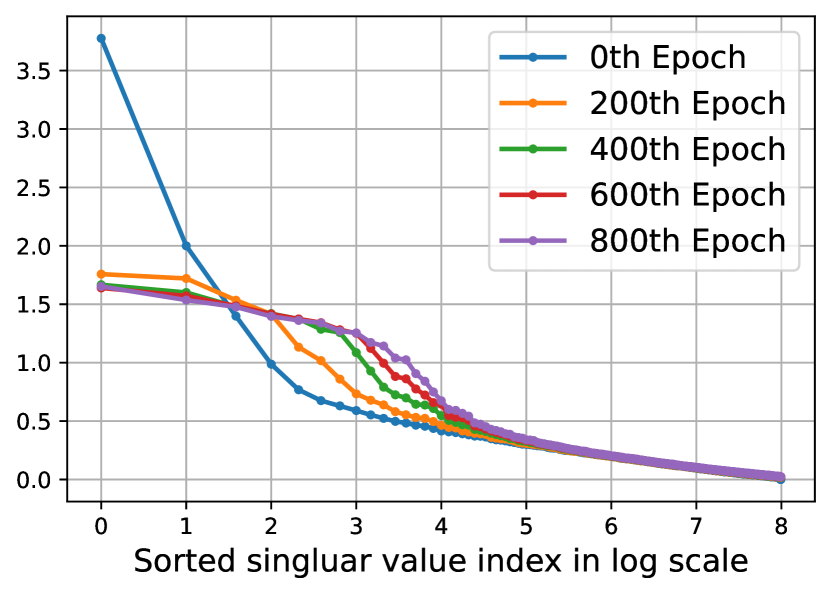
Figure 5: Spectrum of $\tilde{\mathbf{H}}$ when training on Cora with SFA.

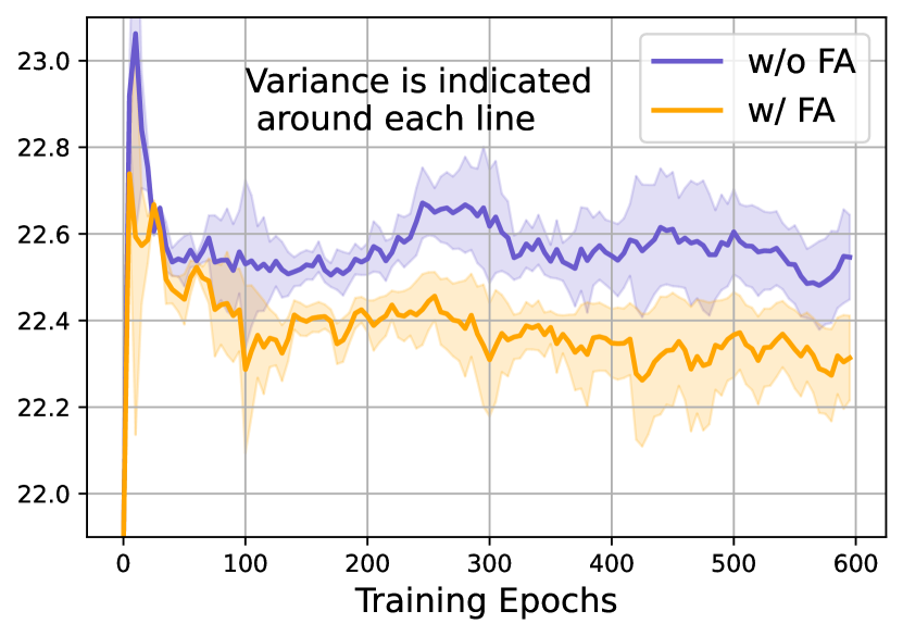
Figure 6: Alignment of f. maps of two views (lower is better).

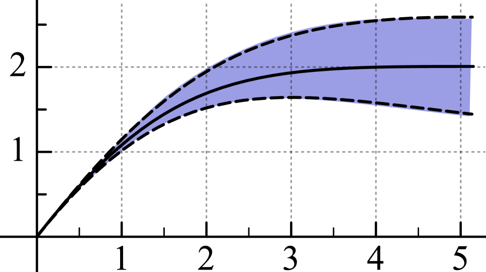
(a) SFA

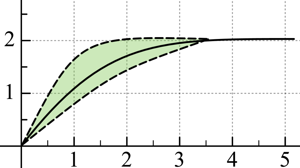
(b) MaxExp(F)

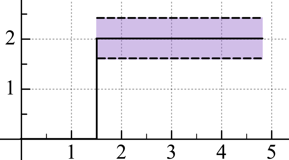
(c) Grassman

Figure 7: Spectrum augmentation variants (dashed lines: injected noise var.) Power Norm. & Power Norm.^∗ resemble (b) and (a).

Robustness to Noisy Features. Below we check on Cora and CiteSeer if GCL with SFA is robust to noisy node features in node classification setting. We draw noise $\Delta\mathbf{x}\sim\mathcal{N}(0,\mathbf{I})$ and inject it into the original node features as $\mathbf{x}+\epsilon\Delta\mathbf{x}$, where $\epsilon\!\geq\!0$ controls the noise intensity. Table 9 shows that SFA is robust to the noisy features. SFA partially balances the spectrum (Fig 3(b) and 2(b) ) of leading singular components where the signal lies, while non-leading components where the noise resides are left mostly unchanged by SFA.

Other Variants of Spectral Augmentation. Below, we experiment with other ways of performing spectral augmentation. Figure 7 shows three different push-forward functions: our SFA, MaxExp(F) (Koniusz and Zhang 2020) and Grassman feature maps (Harandi et al. 2015). As MaxExp(F) and Grassman do not inject any spectral noise, we equip them with explicit noise injectors. To determine what is the best form of such an operator, we vary (i) where the noise is injected, (ii) profile of balancing curve. As the push-forward profiles of SFA and MaxExp(F) are similar (Figure 7), we implicitly inject the noise into MaxExp(F) along the non-leading singular values (c.f. leading singular values of SFA).

MaxExp(F) is only defined for symmetric-positive definite matrices. We extend it to feature maps by:

$$\widetilde{\mathbf{H}}\!=\!\mathbf{H}\mathbf{B}\big{(}\mathbf{I}-(\mathbf{I}-\mathbf{A}/\text{Tr}(\mathbf{A}))^{\eta+\Delta\eta}\big{)},$$ (7)

where $\mathbf{A}=(\mathbf{H}^{\top}\mathbf{H})^{0.5}$ and $\mathbf{B}=(\mathbf{H}^{\top}\mathbf{H})^{-0.5}$ are obtained via highly-efficient Newton-Schulz iteration. We draw the random noise $\Delta\eta\!\sim\!\alpha\mathcal{N}(0,1)$ for each $\mathbf{H}$ and control the variance by $\alpha\!>\!0$. We round $\eta+\Delta\eta$ to the nearest integer (MaxExp(F) requires an integer for fast matrix exponentiation) and ensure the integer is greater than zero. See the Derivation of MaxExp(F) section for details.

Matrix Square Root is similar to MaxExp(F) but the soft function flattening the spectrum is replaced with a matrix square root push-forward function. Power Norm. yields:

$$\widetilde{\mathbf{H}} =\mathbf{H}\mathbf{B}\,\text{PowerNorm}(\mathbf{A};\beta\!+\!\Delta{\beta}),$$ (8)

where $0\leq\beta\!+\Delta{\beta}\!\leq 1$ controls the steepness of the balancing push-forward curve. $\Delta{\beta}$ is drawn from the Normal distribution (we choose the best aug. variance). Power Norm.^∗ is:

$$\!\!\!\!\widetilde{\mathbf{H}} =\mathbf{H}\mathbf{B}\big{(}(1-\beta\!-\!\Delta{\beta})\mathbf{A}^{0.5}+(\beta\!+\!\Delta{\beta})\mathbf{A}^{0.5}\mathbf{A}^{0.25}\big{)}$$

$$=\mathbf{H}\mathbf{B}\,\text{PowerNorm}(\mathbf{A};\beta\!+\!\Delta{\beta}),$$ (9)

where $0\!\leq\!1\!+\Delta{\beta}^{*}\!\leq\!2$, $\Delta{\beta}^{*}$ is drawn from the Normal dist. $\mathbf{A}^{0.5}$ and $\mathbf{A}^{0.25}\!=\!\left(\mathbf{A}^{0.5}\right)^{0.5}\!$ are obtained by Newton-Schulz iterations. See Derivation of Matrix Square Root. for details.

Grassman feature maps can be obtained as:

$$\widetilde{\mathbf{H}}\!=\!\mathbf{H}\mathbf{B}\big{(}\mathbf{V}\text{Flat}(\mathbf{\Lambda};\kappa)\mathbf{V}^{\top}\big{)},$$ (10)

where $\text{Flat}(\cdot;\kappa)$ sets $\kappa\!>\!0$ leading singular values to $1+\Delta\bm{\kappa}$ (the rest is 0), and $\Delta\bm{\kappa}\!\sim\!\alpha\mathcal{N}(0,\mathbf{I})$. In experiments we use SVD and random SVD (injects itself some noise) to produce $\mathbf{V}$ and $\mathbf{\Lambda}$ from $\mathbf{A}$. See Derivation of Grassman for details.

Table 10 shows that SFA outperforms MaxExp(F), Power Norm., Power Norm.^∗ and Grassman. As SFA augments parts of spectrum where signal resides (leading singular values) which is better than augmenting non-leading singular values (some noise may reside there) as in MaxExp(F). As Grassman binarizes spectrum, it may reject some useful signal at the boundary between leading and non-leading singular values. Finally, Matrix Preconditioning model reduces the spectral gap, thus rebalances the spectrum (also non-leading part).

Power Iteration	Am-Computer	Cora	CiteSeer
$k=0$	$87.25$	$83.04$	$71.35$
$k=1$	$\mathbf{{\color[rgb]{0,0,1}88.83}}$	${\color[rgb]{0,0,1}\mathbf{85.90}}$	$73.56$
$k=2$	${\color[rgb]{0,0,1}88.72}$	${\color[rgb]{0,0,1}85.59}$	${\color[rgb]{0,0,1}\mathbf{75.3}}$
$k=4$	$88.64$	$85.29$	${74.8}$
$k=8$	$88.27$	$85.23$	${\color[rgb]{0,0,1}74.9}$

Table 8: Results on different $k$ of SFA.

$\epsilon$		$10^{-4}$	$10^{-3}$	$10^{-2}$	$10^{-1}$
Cora	w/o SFA	80.55	70.67	62.85	59.23
	with SFA	83.14	76.56	69.59	62.55
CiteSeer	w/o SFA	67.48	62.32	52.69	42.81
	with SFA	72.12	70.36	60.40	46.44

Table 9: Results on noisy features.

Spectrum Aug.	Am-Comput.	Cora	CiteSeer
SFA (ours)	$\mathbf{{\color[rgb]{0,0,1}88.83}}$	${\color[rgb]{0,0,1}\mathbf{85.90}}$	${\color[rgb]{0,0,1}\mathbf{75.3}}$
MaxExp(F)	$87.13$	$84.19$	$72.85$
MaxExp(F) (w/o noise)	$86.83$	$83.52$	$72.35$
Power Norm.∗	86.7	82.9	70.4
Power Norm.	86.6	82.7	70.2
Power Norm. (w/o noise)	86.3	82.5	69.9
Grassman	$86.23$	$82.57$	$70.15$
Grassman (w/o noise)	$85.83$	$81.17$	$69.85$
Grassman (rand. SVD)	$85.33$	$81.01$	$69.95$
Matrix Precond.	$82.52$	$78.14$	$67.73$

Table 10: Results of various spectral augmentations.

5 Conclusions

We have shown that GCL is not restricted to only link perturbations or feature augmentation. By introducing a simple and efficient spectral feature augmentation layer we achieve significant performance gains. Our incomplete power iteration is very fast. Our theoretical analysis has demonstrated that SFA rebalances the useful part of spectrum, and also augments the useful part of spectrum by implicitly injecting the noise into singular values of both data views. SFA leads to a better alignment with a lower generalization bound.

6 Acknowledgments

We thank anonymous reviewers for their valuable comments. The work described here was partially supported by grants from the National Key Research and Development Program of China (No. 2018AAA0100204) and from the Research Grants Council of the Hong Kong Special Administrative Region, China (CUHK 2410021, Research Impact Fund, No. R5034-18).

Spectral Feature Augmentation for Graph Contrastive Learning and Beyond (Supplementary Material) Yifei Zhang¹, Hao Zhu^2,3, Zixing Song¹, Piotr Koniusz^3,2,∗, Irwin King¹

Appendix A Notations

In this paper, a graph with node features is denoted as $\mathcal{G}=(\mathbf{X},\mathbf{A})$, where $\mathcal{V}$ is the vertex set, $\mathcal{E}$ is the edge set, and $\mathbf{X}\in\mathbb{R}^{n\times d_{x}}$ is the feature matrix (i.e., the $i$-th row of $\mathbf{X}$ is the feature vector $\mathbf{x}_{i}$ of node $v_{i}$) and $\mathbf{A}\in\{0,1\}^{n\times n}$ denotes the adjacency matrix of $G$, i.e., the $(i,j)$-th entry in $\mathbf{A}$ is 1 if there is an edge between $v_{i}$ and $v_{j}$. The degree of node $v_{i}$, denoted as $d_{i}$, is the number of edges incident with $v_{i}$. The degree matrix $\mathbf{D}$ is a diagonal matrix and its $i$-th diagonal entry is $d_{i}$. For a $d$-dimensional vector $\mathbf{x}\in\mathbb{R}^{d},\|\mathbf{x}\|_{2}$ is the Euclidean norm of $\mathbf{x}$. We use ${x}_{i}$ to denote the $i$ th entry of $\mathbf{x}$, and $\operatorname{diag}(\mathbf{x})\in\mathbb{R}^{d\times d}$ is a diagonal matrix such that the $i$-th diagonal entry is $x_{i}$. We use $\mathbf{a}_{i}$ denote the row vector of $\mathbf{A}$ and ${a}_{ij}$ for the $(i,j)$-th entry of $\mathbf{A}$. The trace of a square matrix $\mathbf{A}$ is denoted by $\operatorname{Tr}(\mathbf{A})$, which is the sum along the diagonal of $\mathbf{A}$. We use $\|\mathbf{A}\|_{2}$ to denote the spectral norm of $\mathbf{A}$, which is its largest singular value $\sigma_{\max}$. We use $\|\mathbf{A}\|_{F}$ for the Frobenius Norm, which is $\|\mathbf{A}\|_{\mathrm{F}}=\sqrt{\sum_{i,j}\left|a_{ij}\right|^{2}}=\sqrt{\operatorname{Tr}\left(\mathbf{A^{\top}A}\right)}$.

Appendix B Bounded Noise Matrix.

For completeness, we analyze the relation between the orthonormal bases $\ {\mathbf{V}}$ and $\mathbf{V}$ of $\widetilde{\mathbf{H}}$ and $\mathbf{H}$, the augmentation error bounded by $\eta$, and the distribution of the spectrum. Let $\mathbf{E}=|\widetilde{\mathbf{H}}-\mathbf{H}|$ be the absolute error matrix where $\mathbf{E}_{ij}=|\widetilde{\mathbf{H}}_{ij}-\mathbf{H}_{ij}|\leq\eta$. Let $\{\widetilde{\sigma}_{i}\}$ and $\{\sigma_{i}\}$ be sets of singular values of $\widetilde{\mathbf{H}}$ and $\mathbf{H}$. We derive the following bound.

Proposition 4.

If $\|\mathbf{V}\!-\!\widetilde{\mathbf{V}}\|_{2}\!\leq\!\epsilon$, each element in $\mathbf{E}_{ij}$ (the absolute error) is bounded by $\eta=2\varepsilon\Delta\tilde{\sigma}_{12}/(n\pi+2\varepsilon)$, where $n$ is the number of nodes and $\Delta\tilde{\sigma}_{12}=\widetilde{\sigma}_{1}-\widetilde{\sigma}_{2}$ is the singular value gap of $\widetilde{\mathbf{H}}$.

Proof.

See Proof of Proposition 4 (suppl. material). ∎

Appendix C Proofs of Propositions

Below we present proofs for several propositions that were not included in the main draft.

C.2 Proof of Proposition 1

Proof.

Let $\mathbf{H}=\mathbf{U}\bm{\Sigma}\mathbf{V}^{\top}$ be the SVD of an input feature map, where $\mathbf{U}$ and $\mathbf{V}$ are the right and left orthonormal matrices that contain the singular vectors. As $\mathbf{r}^{(k)}=(\mathbf{H}^{\top}\mathbf{H})^{k}\mathbf{r}^{(0)}$, we have:

$$\mathbf{r}^{(k)}=(\mathbf{H}^{\top}\mathbf{H})^{k}\mathbf{r}^{(0)}=(\mathbf{V}\bm{\Sigma}^{2k}\mathbf{V}^{\top})\mathbf{r}^{(0)}.$$ (11)

Plugging Equation (11) into Equation (3), we obtain:

$$\!\!\!\!\frac{\mathbf{H}\mathbf{r}^{(k)}\mathbf{r}^{(k)\top}}{\|\mathbf{r}^{(k)}\|_{2}^{2}} \!=\!\frac{\mathbf{U}\Sigma\mathbf{V}^{\top}(\mathbf{V}\bm{\Sigma}^{2k}\mathbf{V}^{\top})\mathbf{r}^{(0)}\mathbf{r}^{(0)\top}(\mathbf{V}\bm{\Sigma}^{2k}\mathbf{V}^{\top})}{\mathbf{r}^{0}(\mathbf{V}\bm{\Sigma}^{2k}\mathbf{V}^{\top})(\mathbf{V}\bm{\Sigma}^{2k}\mathbf{V}^{\top})\mathbf{r}^{0}}$$ (12)

$$\!=\!\frac{\mathbf{U}\bm{\Sigma}^{2k+1}\mathbf{V}^{\top}\mathbf{r}^{(0)}\mathbf{r}^{(0)\top}\mathbf{V}\bm{\Sigma}^{2k}\mathbf{V}^{\top}}{\mathbf{r}^{(0)\top}\mathbf{V}\Sigma^{4k}\mathbf{V}^{\top}\mathbf{r}^{(0)}}.\!\!$$

Let $\mathbf{y}=\mathbf{V}^{\top}\mathbf{r}^{(0)}$ and $k\geq 1$ be the number of iterations, then we simplify Eq. (12) as:

$$\frac{\mathbf{H}\mathbf{r}^{(k)}\mathbf{r}^{(k)\top}}{\|\mathbf{r}^{(k)}\|_{2}^{2}}\!=\!\mathbf{U}\mathbf{Q}(\mathbf{y},k)\mathbf{V}^{\top}$$ (13)

where $$\mathbf{Q}(\mathbf{y},k)\!=\!\frac{\bm{\Sigma}^{2k+1}\mathbf{y}\mathbf{y}^{\top}\bm{\Sigma}^{2k}}{\mathbf{y}^{\top}\bm{\Sigma}^{4k}\mathbf{y}}.$$ (14)

As $\mathbf{r}^{(0)}\sim\mathcal{N}(0,\mathbf{I})$ and $\mathbf{V}$ is a unitary matrix, we have $\mathbf{y}=[y_{1},\cdots,y_{d_{h}}]\sim\mathcal{N}(0,\mathbf{I})$. The expectation of $\mathbf{Q}$ is a diagonal matrix, i.e., we have $\mathbb{E}_{\mathbf{y}\sim\mathcal{N}(0,\mathbf{I})}(\mathbf{Q}(\mathbf{y},k))=\text{diag}\big{(}q_{1}(k),q_{2}(k),\cdots,q(k)_{d_{h}}\big{)}$ with:

$$q_{i}(k)=\sigma_{i}\lambda_{i}(k) \text{ where }\lambda_{i}(k)=\mathbb{E}_{\mathbf{y}\sim\mathcal{N}(0;\mathbf{I})}\big{(}\lambda^{\prime}_{i}(\mathbf{y},k)\big{)},\;$$ (15)

$${\text{ and }}\lambda^{\prime}_{i}(\mathbf{y},k)=\text{$\frac{\left(y_{i}\sigma_{i}^{2k}\right)^{2}}{\sum_{l=1}^{d_{h}}\left(y_{l}\sigma_{l}^{2k}\right)^{2}}$}.$$

For brevity, let us drop parameter $k$ where possible. We need to show that $1\geq\lambda_{i}\geq\lambda_{j}\geq 0$ when $\sigma_{i}\geq\sigma_{j}$. Obviously, $1\geq\lambda_{i}\geq 0$, thus we need to show that $\lambda_{i}-\lambda_{j}\geq 0$ (note):

$$\lambda_{i}-\lambda_{j}= \mathbb{E}\left(\frac{\left(y_{i}\sigma_{i}^{2k}\right)^{2}}{\sum_{l=1}^{d_{h}}\left(y_{l}\sigma_{l}^{2k}\right)^{2}}\right)-\mathbb{E}\Bigg{(}\frac{\big{(}y_{j}\sigma_{j}^{2k}\big{)}^{2}}{\sum_{l=1}^{d_{h}}\left(y_{l}\sigma_{l}^{2k}\right)^{2}}\Bigg{)}$$ (16)

$$\geq\sigma_{j}^{4k}\mathbb{E}\left(\frac{y^{2}_{i}-y^{2}_{j}}{\sum_{l=1}^{d_{h}}\left(y_{l}\sigma_{l}^{2k}\right)^{2}}\right)=0.$$

As

$$\mathbb{E}_{\mathbf{y}\sim\mathcal{N}(0;\mathbf{I})}\!\left(\frac{y^{2}_{i}-y^{2}_{j}}{\sum_{l=1}^{d_{h}}\left(y_{l}\sigma_{l}^{2k}\right)^{2}}\right)=$$

$$\mathbb{E}_{\mathbf{y}\sim\mathcal{N}(0;\mathbf{I})}\!\left(\frac{y^{2}_{i}}{\sum_{l=1}^{d_{h}}\left(y_{l}\sigma_{l}^{2k}\right)^{2}}\right)\!-\!\mathbb{E}_{\mathbf{y}\sim\mathcal{N}(0;\mathbf{I})}\!\left(\frac{y^{2}_{j}}{\sum_{l=1}^{d_{h}}\left(y_{l}\sigma_{l}^{2k}\right)^{2}}\right)\!=\!0$$

due to $y_{i}$, $y_{j}$ being i.i.d. random variables sampled from the normal distribution, inequality (16) holds. ∎

C.3 Proof of Proposition 2

Proof.

We split the proof into four steps as follows.

Step 1. Let $\beta_{i}=(\sigma_{i}^{2k})^{2}$. Define random variable $x_{i}(\mathbf{y})=\frac{\beta_{i}y_{i}^{2}}{\beta_{i}y_{i}^{2}+\sum_{l\neq i}\beta_{l}y^{2}_{l}}=\frac{y_{i}^{2}}{y_{i}^{2}+\sum_{l\neq i}\frac{\beta_{l}}{\beta_{i}}y^{2}_{l}}=\frac{u}{u+v_{i}}$ where ${\mathbf{y}\sim\mathcal{N}(0;\mathbf{I})}$, $u=y_{i}^{2}$ and $v_{i}=\sum_{l\neq i}\frac{\beta_{l}}{\beta_{i}}y^{2}_{l}$. Notice that transformation $y_{i}^{2}$ of the random variable ${{y_{i}}\sim\mathcal{N}(0;1)}$ in fact $\chi^{2}(1)$ distributed, i.e., $y_{i}^{2}\sim\chi^{2}(1)=\mathcal{G}(\frac{1}{2},2)$ because $\chi^{2}(t)\equiv\mathcal{G}(\frac{t}{2},2)$ (it is a well-known fact that the $\chi^{2}(t)$ is a special case of the Gamma distribution defined with the scale parameter).

Step 2. Next, finding the exact distribution of $v_{i}$ (a weighted sum of chi squares) is a topic of ongoing studies but highly accurate surrogates exist, i.e., authors of weighted_chi_squares_sup show that $\sum_{l}\zeta_{l}y_{l}^{2}\sim\mathcal{G}\Big{(}\frac{1}{2}\frac{(\sum_{l}\zeta_{l})^{2}}{\sum_{l}\zeta_{l}^{2}},2\frac{\sum_{l}\zeta_{l}^{2}}{\sum_{l}\zeta_{l}}\Big{)}$ for weights $\zeta_{l}\geq 0$ and $\sum_{l}\zeta_{l}>0$, and so we have $v_{i}\sim\mathcal{G}\Big{(}\frac{1}{2}\frac{(\sum_{l\neq i}\beta_{l})^{2}}{\sum_{l\neq i}\beta_{l}^{2}},\frac{2}{\beta_{i}}\frac{\sum_{l\neq i}\beta_{l}^{2}}{\sum_{l\neq i}\zeta_{l}}\Big{)}$.

Step 3. Now, our proof requires determining the distribution of $x_{i}=\frac{u}{u+v_{i}}$ where $u\sim\mathcal{G}(\alpha_{0},\theta_{0})=\mathcal{G}(\frac{1}{2},2)$ and $v_{i}\sim\mathcal{G}(\alpha_{i},\theta_{i})=\mathcal{G}\Big{(}\frac{1}{2}\frac{(\sum_{l\neq i}\beta_{l})^{2}}{\sum_{l\neq i}\beta_{l}^{2}},\frac{2}{\beta_{i}}\frac{\sum_{l\neq i}\beta_{l}^{2}}{\sum_{l\neq i}\zeta_{l}}\Big{)}$. Let $x=\frac{u}{u+v}=\frac{1}{1+b}$ for $u\sim\mathcal{G}(\alpha_{0},\theta)$ and $v\sim\mathcal{G}(\alpha_{i},\theta)$, then the following are well-known results that $x\sim\mathcal{B}(\alpha_{0},\alpha_{i})$ and $b=u/v\sim\mathcal{B}^{\prime}(\alpha_{i},\alpha_{0})$ where $\mathcal{B}$ and $\mathcal{B}^{\prime}$ stand for the Beta distribution and the Standard Beta Prime distribution, respectively. Let $x_{i}=\frac{u}{u+v_{i}}=\frac{1}{1+\gamma_{i}b_{i}},\;0\leq\gamma_{i}\leq\infty$ where $\gamma_{i}=\frac{\theta_{i}}{\theta_{0}}$ (ratio of scalars in Gamma distributions, i.e., $v_{i}\sim\mathcal{G}(\alpha_{i},\theta_{i})$) and $b_{i}=\frac{1-x_{i}}{x_{i}}$ (solving $x_{i}=\frac{1}{1+b_{i}}$ for $b_{i}$). Substituting $b_{i}=\frac{1-x_{i}}{x_{i}}$ into $\frac{1}{1+\gamma_{i}b_{i}}$ yields $z=\frac{x_{i}}{\gamma_{i}+(1-\gamma_{i})x_{i}}$ and since we have to perform the change of variable, we compute (i) $x_{i}=\frac{\gamma_{i}z}{1-(1-\gamma_{i})z}$ and (ii) the Jacobian which takes a simple form $\frac{\partial x_{i}}{\partial z}=\frac{\gamma_{i}}{(\gamma_{i}+(1-\gamma_{i})z)^{2}}$. Finally, we have $x^{\bullet}_{i}(z)=\mathcal{B}(x_{i};\alpha_{0},\alpha_{i})\cdot\lvert\frac{\partial x_{i}}{\partial z}\rvert=\frac{\gamma_{i}}{(\gamma_{i}+(1-\gamma_{i})z)^{2}}\cdot\mathcal{B}\left(\frac{\gamma_{i}z}{1-(1-\gamma_{i})z};\alpha_{0},\alpha_{i}\right)$. As $\alpha_{0}=\frac{1}{2}$ and $\theta_{0}=2$, we have $\gamma_{i}=\frac{1}{\beta_{i}}\frac{\sum_{l\neq i}\beta_{l}^{2}}{\sum_{l\neq i}\zeta_{l}}$, $\theta_{i}=2\gamma_{i}$ (following our earlier assumptions on modeling $v_{i}$), and the PDF underlying our spectrum-balancing algorithm is $x^{\bullet}_{i}(z)=\frac{\gamma_{i}}{(\gamma_{i}+(1-\gamma_{i})z)^{2}}\cdot\mathcal{B}\Big{(}\frac{\gamma_{i}z}{1-(1-\gamma_{i})z};\frac{1}{2},\alpha_{i}\Big{)}$. Moreover, the above PDF enjoys the support $z\in[0;1]$ because $\mathcal{B}(x_{i})$ enjoys the support $x_{i}\in[0;1]$ and function $x_{i}:[0;1]\longmapsto[0;1]$.

Step 4. Finally, $\lambda_{i}=\mathbb{E}(z)=\int_{0}^{1}z\cdot x^{\bullet}_{i}(z)\,\mathrm{d}z$ is simply obtained by the integration using the Mathematica software followed by a few of algebraic simplifications regarding switching the so-called regularized Hypergeometric function with the so-called Hypergeometric function. ∎

C.4 Proof of Proposition 3

Proof.

Variance $\omega^{2}_{i}=\mathbb{E}(z^{2})-(\mathbb{E}(z))^{2}=\int_{0}^{1}z^{2}\cdot x^{\bullet}_{i}(z)\,\mathrm{d}z-\lambda^{2}_{i}$ relies on the PDF expression $x^{\bullet}_{i}(z)$ derived in the Proof C.3. Expression $\int_{0}^{1}z^{2}\cdot x^{\bullet}_{i}(z)\,\mathrm{d}z$ is simply obtained by the integration using the Mathematica software followed by a few of algebraic simplifications regarding switching the so-called regularized Hypergeometric function with the so-called Hypergeometric function. ∎

C.5 Proof of Proposition 4

Proof.

Since $\|\mathbf{E}\|_{2}^{2}\leq\|\mathbf{E}\|^{2}_{F}\leq n^{2}\tau^{2}$, we have:

$$\|\mathbf{E}\|_{2}\leq n\tau.$$ (17)

From works kostrykin2003subspace_sup,wang2008manifold_sup, we know that if $\widetilde{\mathbf{H}}$ and $\mathbf{E}$ are self-adjoint operators on a separable Hilbert space, then the spectrum of $\mathbf{H}$ is in the closed $\|\mathbf{E}\|-$neighborhood of the spectrum of $\widetilde{\mathbf{H}}$. Thus, we have the following inequality:

$$\|\mathbf{V}^{\perp}\mathbf{V}^{\prime}\|_{2}\leq\pi\|\mathbf{E}\|_{2}/2\Delta\tilde{\sigma},$$ (18)

As we know $\widetilde{\mathbf{H}}$ has the singular value gap $\Delta\tilde{\sigma}_{12}$ We need to assume $\|\mathbf{E}\|_{2}<\Delta\tilde{\sigma}/2$ to guarantee $\mathbf{H}$ also has the singular value gap. Thus, Equation (18) becomes:

$$\|\mathbf{V}^{\perp}\widetilde{\mathbf{V}}\|_{2}\leq\pi\|\mathbf{E}\|_{2}/2(\Delta\tilde{\sigma}_{12}-\|\mathbf{E}\|_{2}).$$ (19)

Similarly, we also have:

$$\|\mathbf{V}\widetilde{\mathbf{V}}^{\perp}\|_{2}\leq\pi\|\mathbf{E}\|_{2}/2(\Delta\tilde{\sigma}_{12}-\|\mathbf{E}\|_{2}).$$ (20)

Since $\|\mathbf{V}-\widetilde{\mathbf{V}}\|_{2}=\max(\|\mathbf{V}\widetilde{\mathbf{V}}^{\perp}\|_{2},\|\mathbf{V}^{\perp}\widetilde{\mathbf{V}}\|_{2})$, we have the following bound:

$$\|\mathbf{V}-\widetilde{\mathbf{V}}\|_{2}\leq\pi\|\mathbf{E}\|_{2}/2(\Delta\tilde{\sigma}_{12}-\|\mathbf{E}\|_{2}).$$ (21)

Equation (21) implies if $\|\widetilde{\mathbf{V}}-\mathbf{V}\|_{2}<\epsilon$, we get $\|\mathbf{E}\|_{2}\leq 2\Delta\tilde{\sigma}_{12}\varepsilon/(2\varepsilon+\pi)$. Combined with Equation (17), we arrive at the conclusion that if the difference of $\|\mathbf{V}-\widetilde{\mathbf{V}}\|_{2}$ is at most $\epsilon$, the absolute error of each element in $\mathbf{E}$ is bounded by $\tau$ and $\tau\leq 2\varepsilon\Delta\tilde{\sigma}_{12}/(n(\pi+2\varepsilon))$. ∎

C.6 Proof of Theorem 1

Proof.

Definition 1.

DBLP:journals/corr/abs-2111-00743_sup $((\sigma,\delta)$-Augmentation). The data augmentation set $\mathcal{A}$ is called a $(\sigma,\delta)$-augmentation, if for each class $C_{k}$, there exists a subset $C_{k}^{0}\subseteq C_{k}$ (called the main part of $C_{k}$ ) such that the following two conditions hold: (i) $\mathbb{P}\left[\mathbf{x}\in C_{k}^{0}\right]\geq\sigma\mathbb{P}\left[\mathbf{x}\in C_{k}\right]$ where $\sigma\in(0,1]$, (ii) $\sup_{\mathbf{x}_{1},\mathbf{x}_{2}\in C_{k}^{0}}d_{\mathcal{A}}\left(\mathbf{x}_{1},\mathbf{x}_{2}\right)\leq\delta$.

Lemma 2.

DBLP:journals/corr/abs-2111-00743_sup For a $(\sigma,\delta)$-augmentation with main part $C_{k}^{0}$ of each class $C_{k}$, if all samples belonging to $\left(C_{1}^{0}\cup\cdots\cup C_{K}^{0}\right)\cap S_{\varepsilon}$ can be correctly classified by a classifier $G$, then its downstream error rate $\operatorname{Err}(G)\leq$ $(1-\sigma)+R_{\varepsilon}$. $R_{\varepsilon}:=\mathbb{P}\left[{S_{\varepsilon}}\right]$ and $S_{\varepsilon}:=\{\mathbf{x}\in\cup_{k=1}^{K}C_{k}:\forall\mathbf{x}_{1},\mathbf{x}_{2}\in\mathcal{A}(\mathbf{x}),\left\|f\left(\mathbf{x}_{1}\right)-f\left(\mathbf{x}_{2}\right)\right\|\geq\varepsilon\}$.

Because $\left\|f\left(\mathbf{x}_{1}\right)-f\left(\mathbf{x}_{2}\right)\right\|$ is a non-negative random variable. Then, for any $\epsilon>0$, according to markov inequality we have:

$$\mathbb{P}[\left\|f\left(\mathbf{x}_{1}\right)-f\left(\mathbf{x}_{2}\right)\right\|_{2}^{2}\geq\epsilon^{2}]$$ (22)

$$\leq{\mathbb{E}_{\mathbf{x}_{1},\mathbf{x}_{2}\in\mathcal{A}(\mathbf{x})}[\left\|f\left(\mathbf{x}_{1}\right)-f\left(\mathbf{x}_{2}\right)\right\|_{2}^{2}]}/{\epsilon^{2}}.$$

Let $f(\mathbf{x})=1$ and $\mathbb{E}_{\mathbf{x}_{1},\mathbf{x}_{2}\in\mathcal{A}(\mathbf{x})}[\left\|f\left(\mathbf{x}_{1}\right)-f\left(\mathbf{x}_{2}\right)\right\|_{2}^{2}]=2-2\mathbb{E}_{\mathbf{x}_{1},\mathbf{x}_{2}\in\mathcal{A}(\mathbf{x})}[f\left(\mathbf{x}_{1}\right)^{\top}f\left(\mathbf{x}_{2}\right)]=2-2\mathcal{L}_{a}$. And thus we have $R_{\varepsilon}\!\!=\!\!P_{\mathbf{x}_{1},\mathbf{x}_{2}\in\mathcal{A}(\mathbf{x})}\{\|f\left(\mathbf{x}_{1}\right)\!-\!f\left(\mathbf{x}_{2})\|\!\geq\!\varepsilon\right\}\!\leq\!\frac{\sqrt{2-2\mathcal{L}_{a}}}{\varepsilon}$. ∎

C.7 Upper bound of $\phi$

As SFA seeks to remove the contribution of the largest singular value of $\mathbf{H}$ from the spectrum $\sigma_{1}\geq\sigma_{2}\geq\cdots\geq\sigma_{d_{h}}$ of $\mathbf{H}$, it follows that for $\sigma_{i}$ we have the upper bound on the push-forward function such that $\phi(\sigma_{i};k)\leq\bar{\phi}(\sigma_{i})-\mathcal{O}(k)$ where $\bar{\phi}(\sigma_{i})=\min(\sigma_{i},\max\limits_{j\neq i}(\sigma_{j}))$ and $\mathcal{O}(k)\geq 0$.

Figure 8 illustrates the above bound. As is clear, the lower the value $k$ is, the more ample is the possibility to tighten that bound (the gap to tighten is captured by $\mathcal{O}(k)\geq 0$).

Nonetheless, with this simple upper bound, we show that we clip/balance spectrum and so the loss in Eq. (6) enjoys lower energy than the loss in Eq. (5), on which Theorem 1 relies.

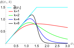
Figure 8: Illustration of $\phi(\sigma_{1};k)$ vs. $\bar{\phi}(\sigma_{1})$.

Notice that the upper bound in Figure 8 is also known as the so-called AxMin pooling operator s19_sup.

C.8 Derivation of MaxExp(F)

Derivation of MaxExp(F) in Eq. (7) is based on the following steps. Based on SVD, we define $\mathbf{H}=\mathbf{U}\mathbf{\Sigma}\mathbf{V}^{\top}$, where $\mathbf{U}$ and $\mathbf{V}$ are left and right singular vectors of $\mathbf{H}$ and $\mathbf{\Sigma}$ are singular values placed along the diagonal.

Let $\mathbf{A}^{2}\!=\!\mathbf{H}^{\top}\mathbf{H}\!=\!\mathbf{V}\mathbf{\Sigma}^{2}\mathbf{V}^{\top}$ and $\mathbf{A}\!=\!\big{(}\mathbf{H}^{\top}\mathbf{H})^{0.5}\!=\!\mathbf{V}\mathbf{\Sigma}\mathbf{V}^{\top}$. Let $\mathbf{B}^{2}\!=\!(\mathbf{H}^{\top}\mathbf{H})^{-1}\!=\!\mathbf{V}\mathbf{\Sigma}^{-2}\mathbf{V}^{\top}$ and $\mathbf{B}\!=\!\big{(}\mathbf{H}^{\top}\mathbf{H}\big{)}^{-0.5}\!=\!\mathbf{V}\mathbf{\Sigma}^{-1}\mathbf{V}^{\top}$.

We apply MaxExp(F) from s17_supp,maxexp_sup,hosvd_sup to $\mathbf{A}$, that is:

$$\mathbf{C} =\big{(}\mathbf{I}-(\mathbf{I}-\mathbf{A}/\text{Tr}(\mathbf{A}))^{\eta+\Delta\eta}\big{)}$$ (23)

$$=\mathbf{V}\big{(}\mathbf{I}-(\mathbf{I}-\mathbf{\Sigma}/\text{Tr}(\mathbf{\Sigma}))^{\eta+\Delta\eta}\big{)}\mathbf{V}^{\top}.$$

Multiplying $\mathbf{C}$ from the left side by $\mathbf{H}\mathbf{B}$, i.e., $\widetilde{\mathbf{H}}=\mathbf{H}\mathbf{B}\mathbf{C}$ yields:

$$\widetilde{\mathbf{H}} =\mathbf{U}\mathbf{\Sigma}\mathbf{V}^{\top}\mathbf{V}\mathbf{\Sigma}^{-1}\mathbf{V}^{\top}\mathbf{V}\big{(}\mathbf{I}-(\mathbf{I}-\mathbf{\Sigma}/\text{Tr}(\mathbf{\Sigma}))^{\eta+\Delta\eta}\big{)}\mathbf{V}^{\top}$$ (24)

$$=\mathbf{U}\big{(}\mathbf{I}-(\mathbf{I}-\mathbf{\Sigma}/\text{Tr}(\mathbf{\Sigma}))^{\eta+\Delta\eta}\big{)}\mathbf{V}^{\top}$$

$$=\mathbf{H}\mathbf{B}\big{(}\mathbf{I}-(\mathbf{I}-\mathbf{A}/\text{Tr}(\mathbf{A}))^{\eta+\Delta\eta}\big{)}$$

$$=\mathbf{H}\mathbf{B}\,\text{MaxExp}(\mathbf{A};\eta+\Delta\eta).$$

Matrices $\mathbf{A}=(\mathbf{H}^{\top}\mathbf{H})^{0.5}$ and $\mathbf{B}=(\mathbf{H}^{\top}\mathbf{H})^{-0.5}$ are obtained via highly-efficient Newton-Schulz iterations higham2008functions_sup,ns_sup in Algorithm 2 given $\zeta=10$ iterations. Figure 7(b) shows the push-forward function

$$\text{MaxExp}(\sigma_{i};\eta,\Delta\eta)=1-\Big{(}1-\frac{\sigma_{i}}{\sum_{j}\sigma_{j}}\Big{)}^{\eta+\Delta\eta},$$ (25)

whose role is to rebalance the spectrum ($\sigma_{i}$ are coefficients on the diagonal of $\mathbf{\Sigma}$).

Algorithm 2 Newton-Schulz iterations.

Input: Symmetric positive-definite matrix $\mathbf{M}=\mathbf{H}^{\top}\mathbf{H}$, total iterations $\zeta$.
Output: Matrices $\mathbf{A}=(\mathbf{H}^{\top}\mathbf{H})^{0.5}$ and $\mathbf{B}=(\mathbf{H}^{\top}\mathbf{H})^{-0.5}$.

1:$\mathbf{M}^{\prime}=\mathbf{M}/\text{Tr}(\mathbf{M})$

2:$\mathbf{P}=\frac{1}{2}(3\mathbf{I}-\mathbf{M}^{\prime})$, $\mathbf{Y}_{0}=\mathbf{M}^{\prime}\mathbf{P}$, $\mathbf{Z}_{0}=\mathbf{P}$

3:for $i=1$ to $\mathrm{\zeta}$ do

4:   $\mathbf{P}=\frac{1}{2}(3\mathbf{I}-\mathbf{Z}_{i-1}\mathbf{Y}_{i-1})$ 

5:   $\mathbf{Y}_{i}=\mathbf{Y}_{i-1}\mathbf{P}$, $\mathbf{Z}_{i}=\mathbf{P}\mathbf{Z}_{i-1}$ 

6:end for

7:$\mathbf{A}=\mathbf{P}\sqrt{\mathrm{Tr}(\mathbf{M})}$ and $\mathbf{B}=\mathbf{Y}_{\zeta}/\sqrt{\mathrm{Tr}(\mathbf{M})}$.

C.9 Derivation of Grassman

Derivation of Grassman feature map in Eq. (10) follows the same steps as those described in the Derivation of MaxExp(F) section above. The only difference is that the soft function flattening the spectrum is replaced with its binarized variant illustrated in Figure 7(c) describing a push-forward function:

$$\text{Flat}(\sigma_{i};\kappa,\Delta\bm{\kappa})=\begin{cases}1+\Delta\kappa_{i}&\text{if $i\leq\kappa$}\\ 0&\text{otherwise},\end{cases}$$ (26)

where $\Delta\kappa_{i}$ are coefficients of $\Delta\bm{\kappa}$ random vector drawn from from the Normal distribution (we choose the best augmentation variance) per sample, and $\kappa>0$ controls the spectrum cut-off.

C.10 Derivation of Matrix Square Root.

Another approach towards spectrum rebalancing we try is based on derivations in the Derivation of MaxExp(F) section above. The key difference is that the soft function flattening the spectrum is replaced with a matrix square root push-forward function:

$$\text{PowerNorm}(\sigma_{i};\beta,\Delta\bm{\beta})$$

$$\quad=(1-\beta-\Delta{\beta})\sigma_{i}^{0.5}+(\beta+\Delta{\beta})\sigma_{i}^{0.75},$$ (27)

where $0\leq\beta\leq 1$ controls the steepness of the balancing push-forward curve and $\Delta{\beta}$ is drawn from the Normal distribution (we choose the best augmentation variance). We ensure that $0\leq\beta+\Delta{\beta}\leq 1$. In practice, we achieve the above function by Newton-Schulz iterations. Specifically, we have:

$$\!\!\!\!\widetilde{\mathbf{H}} =\mathbf{H}\mathbf{B}\big{(}(1-\beta\!-\!\Delta{\beta})\mathbf{A}^{0.5}+(\beta\!+\!\Delta{\beta})\mathbf{A}^{0.5}\mathbf{A}^{0.25}\big{)}$$

$$=\mathbf{H}\mathbf{B}\,\text{PowerNorm}(\mathbf{A};\beta\!+\!\Delta{\beta}),$$ (28)

where $\mathbf{A}^{0.5}$ and $\mathbf{A}^{0.25}=\left(\mathbf{A}^{0.5}\right)^{0.5}$ are obtained by Newton-Schulz iterations.

Appendix D Dataset Description

Below, we describe the datasets and their statistics in detail:

• Cora, CiteSeer, PubMed. These are well-known citation network datasets, in which nodes represent publications and edges indicate their citations. All nodes are labeled according to paper subjects kipf2016semi_sup.

• WikiCS. It is a network of Wikipedia pages related to computer science, with edges showing cross-references. Each article is assigned to one of 10 subfields (classes), with characteristics computed using the content’s averaged GloVe embeddings mernyei2020wiki_sup.

• Am-Computer, AM-Photo. Both of these networks are based on Amazon’s co-purchase data. Nodes represent products, while edges show how frequently they were purchased together. Each product is described using a Bag-of-Words representation based on the reviews (node features). There are ten node classes (product categories) and eight node classes (product categories), respectively mcauley2015image_sup.

Table 11: The dataset statistics.

Dataset	Type	Edges	Nodes	Attributes	Classes
Amazon-Computers	co-purchase	245,778	13,381	767	10
Amazon-Photo	co-purchase	119,043	7,487	745	8
WikiCS	reference	216,123	11,701	3,703	10
Cora	Citation	4,732	3,327	3,327	6
CiteSeer	Citation	5,429	2,708	1,433	7

D.1 Implementation Details

Image Classification. We use ResNet-18 as the backbone for image classification. We run 1000 epochs for CIFAR dataset and 400 epochs for imagenet-100. We follow the hyperparemeter setting in  JMLR:v23:21-1155_sup.

D.2 Hyper-parameter Setting for node classification and clustering

Below, we describe the hyperparameters we use for the main result. They are shown in Table 12.

Dataset	Hidden dims.	Projection Dims.	Learning rate	Training epochs	$\mathbf{k}$	$\mathbf{\tau}$	Acivation func.
Cora	$256$	$256$	$0.0001$	$1,000$	$1$	$0.4$	ReLU
CiteSeer	$256$	$256$	$0.001$	$500$	$2$	$0.9$	ReLU
Am-Computer	$128$	$128$	$0.01$	$2,000$	$1$	$0.2$	ReELU
Am-Photo	$256$	$64$	$0.1$	$2,000$	$1$	$0.3$	ReLU
WikiCS	$256$	$256$	$0.01$	$3,000$	$1$	$0.4$	PReLU

Table 12: The hyperparameters used for reproducing our results.

D.3 Baseline Setting

Table 13 shows the augmentation and constrictive objective setting of the major baseline of GSSL. Graph augmentations include: Edge Removing (ER), Personalized PageRank (PPR), Feature Masking (FM) and Node shuffling(NS). The contrastive objectives include: Information Noise Contrastive Estimation (InfoNCE), Jensen-Shannon Divergence (JSD), the Bootstrapping Latent loss (BL) and Barlow Twins (BT) loss.

Method	Graph Aug.	Spectral Feature Aug.	Contrastive Loss
DGI	NS	$/$	JSD
MVGRL	PPR	$/$	JSD
GRACE	ER+FM	$/$	InfoNCE
GCA	ER+FM	$/$	InfoNCE
BGRL	ER+FM	$/$	BL
G-BT	ER+FM	$/$	BT
SFA${}_{\text{InfoNCE}}$	ER+MF	$\checkmark$	InfoNCE
SFA${}_{\text{BT}}$	ER+MF	$\checkmark$	BT

Table 13: The setting of augmentation and contrastive objective of the major baseline and our approach.

Appendix E Additional Empirical Results

Node Clustering. We also evaluate the proposed method on node clustering on Cora, Citeseer, and Am-computer datasets. We compare our model with t variational GAE (VGAE) kipf2016variational_sup, GRACE DBLP:journals/corr/grace_sup, and G-BT bielak2021graph_sup. We measure the performance by the clustering Normalized Mutual Information (NMI) and Adjusted Rand Index (ARI). We run each method 10 times. Table 14 shows that our model achieves the best NMI and ARI scores on all benchmarks. To compare with a recently published contrastive model (i.e., SUGLR mo2022simple_sup and MERIT jin2021multi_sup)), we combine SFA with these models and report their accuracy in Table 15.

	Am-Computer		Cora		CiteSeer
Method	NMI%	ARI%	NMI%	ARI%	NMI%	ARI%
K-means	$19.2\pm 1.9$	$8.6\pm 1.3$	$22.50\pm 1.2$	$22.1\pm 2.1$	$18.04\pm 1.4$	$18.33\pm 1.8$
GAE	$44.1\pm 0.0$	$25.8\pm 1.0$	$30.82\pm 1.2$	$25.47\pm 0.9$	$24.05\pm 1.4$	$20.56\pm 0.8$
VGAE	$42.6\pm 0.1$	$24.6\pm 0.1$	$32.92\pm 1.2$	$26.47\pm 1.1$	$26.05\pm 0.9$	$23.56\pm 0.8$
GRACE	$42.6\pm 2.1$	$24.6\pm 1.3$	$57.00\pm 1.2$	$53.74\pm 1.5$	$46.12\pm 1.3$	$44.50\pm 1.1$
G-BT	$41.0\pm 1.9$	$23.4\pm 1.4$	$54.90\pm 2.2$	$55.20\pm 1.6$	$45.00\pm 2.3$	$44.10\pm 2.1$
SFA${}_{\text{BT}}$	${\color[rgb]{0,0,1}45.4\pm 2.1}$	${\color[rgb]{0,0,1}\mathbf{28.3\pm 2.0}}$	${\color[rgb]{0,0,1}55.91\pm 2.3}$	${\color[rgb]{0,0,1}55.36\pm 1.7}$	${\color[rgb]{0,0,1}46.46\pm 2.3}$	${\color[rgb]{0,0,1}\mathbf{45.37\pm 1.8}}$
SFA${}_{\text{InfoNCE}}$	${\color[rgb]{0,0,1}\mathbf{46.2\pm 2.2}}$	${\color[rgb]{0,0,1}27.4\pm 1.7}$	${\color[rgb]{0,0,1}\mathbf{58.91}\pm 1.1}$	${\color[rgb]{0,0,1}\mathbf{56.96\pm 1.6}}$	${\color[rgb]{0,0,1}\mathbf{46.96\pm 1.5}}$	${\color[rgb]{0,0,1}44.97\pm 1.8}$

Table 14: Node Clustering result on Am-Computer, Cora, CiteSeer. (Note that SFA${}_{\text{InfoNEC}}$ and SFA${}_{\text{BT}}$ can be directly compared with GRACE and G-BT respectively.)

Accuracy	AM-Comp.	Cora	Citeseer
K-means	$37.3$	$34.6$	$38.4$
GAE	$54.0$	$41.2$	$41.2$
VGAE	$55.4$	$55.9$	$44.3$
MERIT	$64.2$	$72.6$	$69.8$
SFA${}_{\text{MERIT}}$	$\bf{\color[rgb]{0,0,1}66.2}$	$\bf{\color[rgb]{0,0,1}74.6}$	$\bf{\color[rgb]{0,0,1}70.9}$
MVGRL	$63.1$	$73.4$	$70.1$
SFA${}_{\text{MVGRL}}$	$\bf{\color[rgb]{0,0,1}66.0}$	$\bf{\color[rgb]{0,0,1}73.9}$	$\bf{\color[rgb]{0,0,1}70.7}$
G-BT	$62.4$	$65.6$	$67.1$
SFA${}_{\text{BT}}$	$\bf{\color[rgb]{0,0,1}65.6}$	$\bf{\color[rgb]{0,0,1}67.4}$	$\bf{\color[rgb]{0,0,1}68.2}$
GRACE	$64.4$	$66.6$	$68.1$
SFA${}_{\text{InfoNCE}}$	$\bf{\color[rgb]{0,0,1}66.3}$	$\bf{\color[rgb]{0,0,1}69.5}$	$\bf{\color[rgb]{0,0,1}69.2}$
SUGRL	$65.2$	$73.2$	$70.5$
SFA${}_{\text{SUGRL}}$	$\bf{\color[rgb]{0,0,1}66.7}$	$\bf{\color[rgb]{0,0,1}74.4}$	$\bf{\color[rgb]{0,0,1}70.7}$

Table 15: Node Clustering (accuracy %).

Improved Alignment. We show more results of how SFA improves the alignment of two views during training (see Fig. 9).

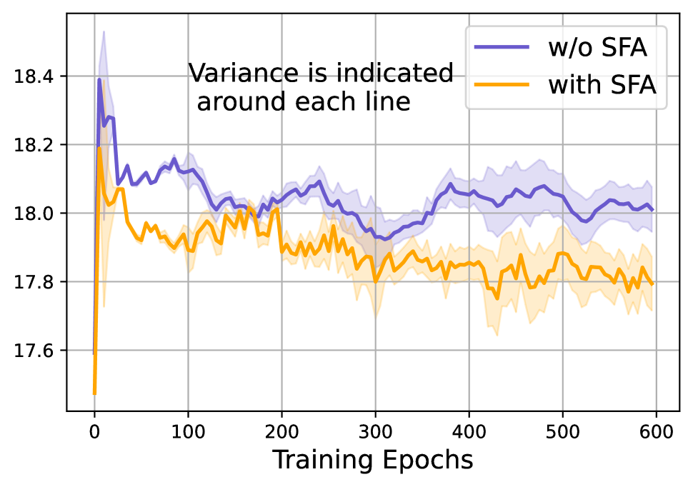
(a) CiteSeer

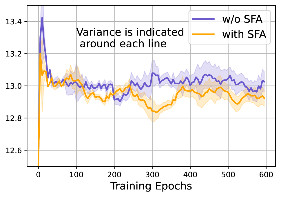
(b) WikiCS

Figure 9: Additional result on improved alignment on CiteSeer and WikiCS. Y-axis denote the alignment which is computed by $\|\mathbf{H}^{\alpha}-\mathbf{H}^{\beta}\|^{2}_{F}$ (or $\|\tilde{\mathbf{H}}^{\alpha}-\tilde{\mathbf{H}}^{\beta}\|^{2}_{F}$). The lower the curve the better.

Appendix F Matrix Preconditioning

Method	Cora	CiteSeer	PubMed
Matrix Precond. (by LU factorization)	$78.1\pm 0.2$	$67.7\pm 0.3$	$83.4\pm 0.1$
Grassman (w/o noise) ($\kappa=15$)	$81.1\pm 0.2$	$72.3\pm 0.3$	$83.2\pm 0.2$
PCA	$80.0\pm 0.1$	$70.5\pm 0.5$	$81.5\pm 0.3$
SFA${}_{\text{infoNCE}}$	$\bf 86.43\pm 0.1$	$\bf 76.1\pm 0.3$	$\bf 86.2\pm 0.2$

Table 16: Comparison of SFA with Matrix Precond., Grassman feature map, and PCA.

Matrix Preconditioning (MP). For the discussion on Matrix Preconditioning (MP) techniques, “Matrix Preconditioning Techniques and Applications” book chen2005matrix_sup shows how to design an effective preconditioner matrix $\mathbf{M}$ in order to obtain a numerical solution for solving a large linear system:

$$\mathbf{Ax}=\mathbf{b}\rightarrow\mathbf{MAx}=\mathbf{Mb}$$ (29)

The goal of Matrix Preconditioning is to make $\tilde{\mathbf{A}}=\mathbf{MA}$ to have small conditional number $p=\sigma_{\text{max}}/\sigma_{\text{min}}$, (e.g., $\mathbf{M}\approx\mathbf{A^{-1}}$ and $\tilde{\mathbf{A}}\approx\mathbf{I}$) so that solving $\mathbf{MAx}=\mathbf{Mb}$ is much easier, faster and more accurate than solving $\mathbf{Ax}=\mathbf{b}$.

Spectrum rebalancing via MP. Since the $\tilde{\mathbf{A}}$ has small condition number $p=\sigma_{\text{max}}/\sigma_{\text{min}}$, MP may somehow achieve similar effect on balancing the spectrum. We set ${\bf A=\mathbf{H}^{\top}\mathbf{H}}$ as ${\bf A}$ is required to be SPD (needs to be invertible) which additionally complicates recovery of the rectangular feature matrix $\tilde{\bf H}$ from $\mathbf{MA}$. MP requires inversions for which backpropagation through SVD is unstable (SVD backpropagation fails under so-called non-simple eigenvalues due to undetermined solution).

Below we provide clear empirical results and compare our method to Matrix Preconditioning, Grassman feature map (without noise injection) and PCA (Table 16). Specifically:

• We recover the augmented feature $\tilde{\mathbf{H}}$ from $\tilde{\mathbf{H}}^{\top}\tilde{\mathbf{H}}=\mathbf{MH}^{\top}\mathbf{H}$ where the preconditioner $\mathbf{M}=\mathbf{U}^{-1}\mathbf{L}^{-1}$ (where $\mathbf{L}$, $\mathbf{U}$ is the LU factorization of $\mathbf{H}^{\top}\mathbf{H}$).

• Judging from the role preconditioner ${\bf M}$ fulfills (fast convergence of the linear system), ${\bf M}$ cannot solve our problem, i.e., it cannot flatten some $\kappa>0$ leading singular values (where signal most likely resides) while leaving remaining singular values unchanged (our method achieves that as Fig. 3(b) of the main paper shows).

• Grassmann feature map which forms subspace from $\kappa>0$ leading singular values is in fact closer “in principle” to SFA than MP methods. Thus, we apply SVD and flatten $\kappa$ leading singular values $\sigma_{i}$ while nullifying remaining singular values $\sigma_{i}$.

• We also compare our approach to PCA given the best $\kappa=20$ components.

The impact of subspace size $\kappa$ on results with Grassmann feature maps (without noise injection) is shown in Table 17. Number $\kappa=15$ agrees with our observations that leading 12 to 15 singular values should be flattened (Fig 7 of the main paper).

Our SFA performs better as:

• It does not completely nullify non-leading singular values (some of them are still useful/carry signal).

• It does perform spectral augmentation on the leading singular values.

• SFA does not rely on SVD whose backpropagation step is unstable (e.g., undefined for non-simple singular including zero singular values).

$\kappa$	2	5	10	15	20	30	50	100	250	SFA${}_{\text{infoNCE}}$
	$78.7$	$80.1$	$80.5$	$81.1$	$80.3$	$80.5$	$80.4$	$80.2$	$79.8$	${\color[rgb]{0,0,1}\mathbf{86.4}}$

Table 17: Impact of subspace size $\kappa$ in Grassman feature map without the noise injection (Cora).

It should be noted that most of random MP methods in halko2011finding_sup need to compute the eigenvalues/eigenvectors which is time-consuming even with random SVD, and this performs badly in practice. Suppose $k$ is the iteration number of a random approach, it then requires $O(kq)$ to get top $q$ eigenvectors (e.g., the random SVD in halko2011finding_sup). Then one must manually set eigenvectors to yield equal contribution (i.e., $\sigma_{i}=1$ for all $i$) which is what we do exactly for the Grassmann feature map in Table 17.

Other plausible feature balancing models which are outside of the scope of our work include the so-called democratic aggregation democratic_sup,Lin_2018_ECCV_sup.

Appendix G Why does the Incomplete Iteration of SFA Work? 

Let $\mathbf{M}=\mathbf{H}^{\top}\mathbf{H}$ and let the power iteration be expressed as $\mathbf{M}^{k}\mathbf{r}^{(0)}$ where $\mathbf{r}^{(0)}\sim\mathcal{N}(0;\mathbf{I})$, as in Algorithm 1. Let $\mathbf{M}=\mathbf{V}\mathbf{\Sigma}^{2}\mathbf{V}^{\top}$ be an SVD of $\mathbf{M}$, then the eigenvalue decomposition admits $\mathbf{M}^{k}\mathbf{V}=\mathbf{V}\mathbf{\Sigma}^{2}$. Let $\mathbf{r}^{(0)}=\mathbf{V}\widetilde{\mathbf{r}}^{(0)}$ then $\mathbf{M}^{k}\mathbf{r}^{(0)}=\mathbf{M}^{k}\mathbf{V}\widetilde{\mathbf{r}}^{(0)}=\mathbf{V}\mathbf{\Sigma}^{2k}\widetilde{\mathbf{r}}^{(0)}$. We notice that

$$\mathbf{M}^{k}\mathbf{r}^{(0)} =\sigma_{1}^{2k}\sum_{i}\mathbf{v}_{i}\Big{(}\frac{\sigma_{i}}{\sigma_{1}}\Big{)}^{2k}\widetilde{{r}}_{i}^{(0)}$$ (30)

$$=\sigma_{1}^{2k}\sum_{i}\mathbf{v}_{i}\Big{(}\frac{\sigma_{i}}{\sigma_{1}}\Big{)}^{2k}\langle\mathbf{v}_{i}^{\top},\mathbf{r}^{(0)}\rangle$$

$$=\sum_{i}\gamma_{i}\mathbf{v}_{i},$$

where $\gamma_{i}=\sigma_{1}^{2k}\big{(}\frac{\sigma_{i}}{\sigma_{1}}\big{)}^{2k}\langle\mathbf{v}_{i}^{\top},\mathbf{r}^{(0)}\rangle$ which clearly shows that $\sum_{i}\gamma_{i}\mathbf{v}_{i}$ is a linear combination of more than one $\mathbf{v}_{i}$ if $k\ll\infty$. Notice also that as the smaller $\sigma_{i}$ is compared to the leading singular value $\sigma_{1}$, the quicker the ratio $\Big{(}\frac{\sigma_{i}}{\sigma_{1}}\Big{)}^{2k}$ declines towards zero as $k$ grows (it follows the power law non-linearity in Figure 10). Therefore, leading singular values make a significantly stronger contribution to the linear combination $\sum_{i}\gamma_{i}\mathbf{v}_{i}$ compared to non-leading singular values. Thus, for small $k$, matrix

$$\mathbf{M}_{\text{PowerIter}}=\frac{\mathbf{M}^{k}\mathbf{r}^{(0)}{\mathbf{r}^{(0)}}^{\top}\mathbf{M}^{k}}{\lVert\mathbf{M}^{k}\mathbf{r}^{(0)}\rVert_{2}^{2}}=\frac{\big{(}\sum_{i}\rho_{i}\mathbf{v}_{i}\big{)}\big{(}\sum_{j}\rho_{j}\mathbf{v}_{j}^{\top}\big{)}}{\lVert\sum_{l}\rho_{l}\mathbf{v}_{l}\rVert_{2}^{2}},$$ (31)

is a low-rank matrix “focusing” on leading singular vectors of $\mathbf{M}$ more according to the power law non-linearity in Figure 10. Intuitively, for that very reason, as a typical matrix spectrum of $\mathbf{H}$ (and $\mathbf{M}$) also follows the power law non-linearity, $\mathbf{H}$ is balanced by the inverted power law non-linearity of $\mathbf{I}-\mathbf{M}_{\text{PowerIter}}$. In the above equation, $\rho_{i}=\big{(}\frac{\sigma_{i}}{\sigma_{1}}\big{)}^{2k}\langle\mathbf{v}_{i}^{\top},\mathbf{r}^{(0)}\rangle$.

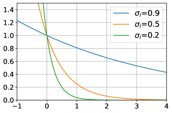
Figure 10: Plot of $\big{(}\frac{\sigma_{i}}{\sigma_{1}}\big{)}^{2k}$ given $\sigma_{1}=1$ exhibits the power law non-linearity.

Appendix H Broader Impact and Limitations

Empowering deep learning with the ability of reasoning and making predictions on the graph-structured data is of broad interest, GCL may be applied in many applications such as recommendation systems, neural architecture search, and drug discovery. The proposed graph contrastive learning framework with spectral feature augmentations is a general framework that can improve the effectiveness and efficiency of graph neural networks through model pre-training. It can also inspire further studies on the augmentation design from a new perspective. Notably, our proposed SFA is a plug-and-play layer which can be easily integrated with existing systems (e.g., recommendation system) at a negligible runtime cost. SFA facilitates training of high-quality embeddings for users and items to resolve the cold-start problem in on-line shopping (and other graph-based applications). One limitation of our method is that our work mainly serves as a plug-in for existing machine learning models and thus it does not model any specific fairness prior. Thus, the GCL model with SFA is still required to prevent the bias of the model (e.g., gender bias, ethnicity bias, etc.), as the provided data itself may be strongly biased during the processes of the data collection, graph construction, etc. Exploring the augmentation with some fairness prior may address such a limitation. We assume is reasonable to let the GCL model tackle the fairness issue.

plainnataaai23sub

References

- Bengio et al. (2013) Bengio, Y.; Mesnil, G.; Dauphin, Y. N.; and Rifai, S. 2013. Better Mixing via Deep Representations. In ICML.
- Bielak, Kajdanowicz, and Chawla (2021) Bielak, P.; Kajdanowicz, T.; and Chawla, N. V. 2021. Graph Barlow Twins: A self-supervised representation learning framework for graphs. ArXiv preprint.
- Chen et al. (2020) Chen, T.; Kornblith, S.; Norouzi, M.; and Hinton, G. E. 2020. A Simple Framework for Contrastive Learning of Visual Representations. In ICML.
- da Costa et al. (2022) da Costa, V. G. T.; Fini, E.; Nabi, M.; Sebe, N.; and Ricci, E. 2022. solo-learn: A Library of Self-supervised Methods for Visual Representation Learning. JMLR.
- Deng et al. (2009) Deng, J.; Dong, W.; Socher, R.; Li, L.; Li, K.; and Li, F. 2009. ImageNet: A large-scale hierarchical image database. In CVPR.
- DeVries and Taylor (2017) DeVries, T.; and Taylor, G. W. 2017. Dataset augmentation in feature space. ArXiv preprint.
- Dobson and Doig (2003) Dobson, P. D.; and Doig, A. J. 2003. Distinguishing enzyme structures from non-enzymes without alignments. Journal of molecular biology, (4).
- Feng et al. (2021) Feng, S. Y.; Gangal, V.; Wei, J.; Chandar, S.; Vosoughi, S.; Mitamura, T.; and Hovy, E. 2021. A Survey of Data Augmentation Approaches for NLP. In Findings of the Association for Computational Linguistics: ACL-IJCNLP 2021.
- Gao, Yao, and Chen (2021) Gao, T.; Yao, X.; and Chen, D. 2021. SimCSE: Simple Contrastive Learning of Sentence Embeddings. In EMNLP.
- Grover and Leskovec (2016) Grover, A.; and Leskovec, J. 2016. Node2vec: Scalable Feature Learning for Networks. In KDD.
- Hafidi et al. (2020) Hafidi, H.; Ghogho, M.; Ciblat, P.; and Swami, A. 2020. GraphCL: Contrastive Self-supervised Learning of Graph Representations. ArXiv preprint.
- Hamilton, Ying, and Leskovec (2017) Hamilton, W. L.; Ying, Z.; and Leskovec, J. 2017. Inductive Representation Learning on Large Graphs. In NeurIPS.
- Harandi et al. (2015) Harandi, M.; Hartley, R.; Shen, C.; Lovell, B.; and Sanderson, C. 2015. Extrinsic Methods for Coding and Dictionary Learning on Grassmann Manifolds. IJCV.
- Hariharan and Girshick (2017) Hariharan, B.; and Girshick, R. B. 2017. Low-Shot Visual Recognition by Shrinking and Hallucinating Features. In ICCV.
- Hassani and Ahmadi (2020) Hassani, K.; and Ahmadi, A. H. K. 2020. Contrastive Multi-View Representation Learning on Graphs. In ICML.
- He et al. (2020) He, K.; Fan, H.; Wu, Y.; Xie, S.; and Girshick, R. B. 2020. Momentum Contrast for Unsupervised Visual Representation Learning. In CVPR.
- Huang, Yi, and Zhao (2021) Huang, W.; Yi, M.; and Zhao, X. 2021. Towards the Generalization of Contrastive Self-Supervised Learning. ArXiv preprint.
- Jin et al. (2021) Jin, M.; Zheng, Y.; Li, Y.-F.; Gong, C.; Zhou, C.; and Pan, S. 2021. Multi-scale contrastive siamese networks for self-supervised graph representation learning. ArXiv preprint.
- Jing et al. (2021) Jing, L.; Vincent, P.; LeCun, Y.; and Tian, Y. 2021. Understanding dimensional collapse in contrastive self-supervised learning. ArXiv preprint.
- Kipf and Welling (2016) Kipf, T. N.; and Welling, M. 2016. Variational graph auto-encoders. ArXiv preprint.
- Kipf and Welling (2017) Kipf, T. N.; and Welling, M. 2017. Semi-Supervised Classification with Graph Convolutional Networks. In ICLR.
- Klicpera, Bojchevski, and Günnemann (2019) Klicpera, J.; Bojchevski, A.; and Günnemann, S. 2019. Predict then Propagate: Graph Neural Networks meet Personalized PageRank. In ICLR.
- Koniusz and Zhang (2020) Koniusz, P.; and Zhang, H. 2020. Power Normalizations in Fine-grained Image, Few-shot Image and Graph Classification. TPAMI.
- Krizhevsky, Hinton et al. (2009) Krizhevsky, A.; Hinton, G.; et al. 2009. Learning multiple layers of features from tiny images.
- McAuley et al. (2015) McAuley, J. J.; Targett, C.; Shi, Q.; and van den Hengel, A. 2015. Image-Based Recommendations on Styles and Substitutes. In SIGIR.
- Mernyei and Cangea (2020) Mernyei, P.; and Cangea, C. 2020. Wiki-cs: A wikipedia-based benchmark for graph neural networks. ArXiv preprint.
- Mo et al. (2022) Mo, Y.; Peng, L.; Xu, J.; Shi, X.; and Zhu, X. 2022. Simple unsupervised graph representation learning. AAAI.
- Page et al. (1999) Page, L.; Brin, S.; Motwani, R.; and Winograd, T. 1999. The PageRank citation ranking: Bringing order to the web. Technical report, Stanford InfoLab.
- Pan et al. (2018) Pan, S.; Hu, R.; Long, G.; Jiang, J.; Yao, L.; and Zhang, C. 2018. Adversarially Regularized Graph Autoencoder for Graph Embedding. In Proceedings of the Twenty-Seventh International Joint Conference on Artificial Intelligence, IJCAI 2018, July 13-19, 2018, Stockholm, Sweden.
- Peng et al. (2020) Peng, Z.; Huang, W.; Luo, M.; Zheng, Q.; Rong, Y.; Xu, T.; and Huang, J. 2020. Graph Representation Learning via Graphical Mutual Information Maximization. In WWW.
- Perozzi, Al-Rfou, and Skiena (2014) Perozzi, B.; Al-Rfou, R.; and Skiena, S. 2014. DeepWalk: online learning of social representations. In KDD.
- Prabowo et al. (2019) Prabowo, A.; Koniusz, P.; Shao, W.; and Salim, F. D. 2019. COLTRANE: ConvolutiOnaL TRAjectory NEtwork for Deep Map Inference. In Proceedings of the 6th ACM International Conference on Systems for Energy-Efficient Buildings, Cities, and Transportation, BuildSys 2019, New York, NY, USA, November 13-14, 2019, 21–30. ACM.
- Riesen and Bunke (2008) Riesen, K.; and Bunke, H. 2008. IAM graph database repository for graph based pattern recognition and machine learning. In Joint IAPR International Workshops on Statistical Techniques in Pattern Recognition (SPR) and Structural and Syntactic Pattern Recognition (SSPR).
- Schwartz et al. (2018) Schwartz, E.; Karlinsky, L.; Shtok, J.; Harary, S.; Marder, M.; Kumar, A.; Feris, R. S.; Giryes, R.; and Bronstein, A. M. 2018. Delta-encoder: an effective sample synthesis method for few-shot object recognition. In NeurIPS.
- Shorten and Khoshgoftaar (2019) Shorten, C.; and Khoshgoftaar, T. M. 2019. A survey on image data augmentation for deep learning. Journal of Big Data, (1).
- Sinha et al. (2015) Sinha, A.; Shen, Z.; Song, Y.; Ma, H.; Eide, D.; Hsu, B.-J.; and Wang, K. 2015. An overview of microsoft academic service (mas) and applications. In WWW.
- Song et al. (2021) Song, Z.; Meng, Z.; Zhang, Y.; and King, I. 2021. Semi-supervised Multi-label Learning for Graph-structured Data. In CIKM, 1723–1733.
- Song, Zhang, and King (2022) Song, Z.; Zhang, Y.; and King, I. 2022. Towards an optimal asymmetric graph structure for robust semi-supervised node classification. In KDD.
- Sun, Koniusz, and Wang (2019) Sun, K.; Koniusz, P.; and Wang, Z. 2019. Fisher-Bures Adversary Graph Convolutional Networks. Conference on Uncertainty in Artificial Intelligence, 115: 465–475.
- Suresh et al. (2021) Suresh, S.; Li, P.; Hao, C.; and Neville, J. 2021. Adversarial Graph Augmentation to Improve Graph Contrastive Learning. ArXiv preprint.
- Thakoor et al. (2021) Thakoor, S.; Tallec, C.; Azar, M. G.; Munos, R.; Veličković, P.; and Valko, M. 2021. Bootstrapped representation learning on graphs. ArXiv preprint.
- Tian et al. (2020) Tian, Y.; Sun, C.; Poole, B.; Krishnan, D.; Schmid, C.; and Isola, P. 2020. What Makes for Good Views for Contrastive Learning? In NeurIPS.
- Upchurch et al. (2017) Upchurch, P.; Gardner, J. R.; Pleiss, G.; Pless, R.; Snavely, N.; Bala, K.; and Weinberger, K. Q. 2017. Deep Feature Interpolation for Image Content Changes. In CVPR.
- Velickovic et al. (2018) Velickovic, P.; Cucurull, G.; Casanova, A.; Romero, A.; Liò, P.; and Bengio, Y. 2018. Graph Attention Networks. In ICLR.
- Velickovic et al. (2019) Velickovic, P.; Fedus, W.; Hamilton, W. L.; Liò, P.; Bengio, Y.; and Hjelm, R. D. 2019. Deep Graph Infomax. In ICLR.
- Wang and Isola (2020) Wang, T.; and Isola, P. 2020. Understanding Contrastive Representation Learning through Alignment and Uniformity on the Hypersphere. In ICML.
- Wang et al. (2019) Wang, Y.; Pan, X.; Song, S.; Zhang, H.; Huang, G.; and Wu, C. 2019. Implicit Semantic Data Augmentation for Deep Networks. In NeurIPS.
- Wei and Zou (2019) Wei, J.; and Zou, K. 2019. EDA: Easy Data Augmentation Techniques for Boosting Performance on Text Classification Tasks. In EMNLP.
- Wu et al. (2019) Wu, F.; Souza, A.; Zhang, T.; Fifty, C.; Yu, T.; and Weinberger, K. 2019. Simplifying Graph Convolutional Networks. In ICML, 6861–6871.
- Xia et al. (2022) Xia, J.; Wu, L.; Chen, J.; Hu, B.; and Li, S. Z. 2022. SimGRACE: A Simple Framework for Graph Contrastive Learning without Data Augmentation. In WWW.
- Yin et al. (2021) Yin, Y.; Wang, Q.; Huang, S.; Xiong, H.; and Zhang, X. 2021. AutoGCL: Automated Graph Contrastive Learning via Learnable View Generators. ArXiv preprint.
- You et al. (2021) You, Y.; Chen, T.; Shen, Y.; and Wang, Z. 2021. Graph Contrastive Learning Automated. In ICML.
- You et al. (2020a) You, Y.; Chen, T.; Sui, Y.; Chen, T.; Wang, Z.; and Shen, Y. 2020a. Graph Contrastive Learning with Augmentations. In NeurIPS.
- You et al. (2020b) You, Y.; Chen, T.; Sui, Y.; Chen, T.; Wang, Z.; and Shen, Y. 2020b. Graph Contrastive Learning with Augmentations. In NeurIPS.
- You et al. (2022) You, Y.; Chen, T.; Wang, Z.; and Shen, Y. 2022. Bringing Your Own View: Graph Contrastive Learning without Prefabricated Data Augmentations. In WSDM.
- Yu, Cai, and Li (2020) Yu, T.; Cai, Y.; and Li, P. 2020. Toward faster and simpler matrix normalization via rank-1 update. In European Conference on Computer Vision, 203–219. Springer.
- Zbontar et al. (2021) Zbontar, J.; Jing, L.; Misra, I.; LeCun, Y.; and Deny, S. 2021. Barlow Twins: Self-Supervised Learning via Redundancy Reduction. In ICML.
- Zhang, Zhang, and Koniusz (2019) Zhang, H.; Zhang, J.; and Koniusz, P. 2019. Few-shot Learning via Saliency-guided Hallucination of Samples. In CVPR, 2770–2779.
- Zhang et al. (2022a) Zhang, S.; Wang, L.; Murray, N.; and Koniusz, P. 2022a. Kernelized Few-Shot Object Detection With Efficient Integral Aggregation. In CVPR, 19207–19216.
- Zhang et al. (2022b) Zhang, Y.; Zhu, H.; Meng, Z.; Koniusz, P.; and King, I. 2022b. Graph-adaptive Rectified Linear Unit for Graph Neural Networks. In Proceedings of the ACM Web Conference 2022, 1331–1339.
- Zhang et al. (2022c) Zhang, Y.; Zhu, H.; Song, Z.; Koniusz, P.; and King, I. 2022c. COSTA: Covariance-Preserving Feature Augmentation for Graph Contrastive Learning. In KDD.
- Zhu and Koniusz (2021) Zhu, H.; and Koniusz, P. 2021. Simple Spectral Graph Convolution. In ICLR.
- Zhu and Koniusz (2022) Zhu, H.; and Koniusz, P. 2022. Generalized Laplacian Eigenmaps. NeurIPS.
- Zhu, Sun, and Koniusz (2021) Zhu, H.; Sun, K.; and Koniusz, P. 2021. Contrastive Laplacian Eigenmaps. NeurIPS.
- Zhu et al. (2021a) Zhu, Y.; Xu, Y.; Liu, Q.; and Wu, S. 2021a. An Empirical Study of Graph Contrastive Learning. ArXiv preprint.
- Zhu et al. (2020) Zhu, Y.; Xu, Y.; Yu, F.; Liu, Q.; Wu, S.; and Wang, L. 2020. Deep Graph Contrastive Representation Learning. ArXiv preprint.
- Zhu et al. (2021b) Zhu, Y.; Xu, Y.; Yu, F.; Liu, Q.; Wu, S.; and Wang, L. 2021b. WWW. In Proceedings of the Web Conference 2021.