Computable bounds for the reach and -convexity of subsets of
Abstract
The convexity of a set can be generalized to the two weaker notions of reach and -convexity; both describe the regularity of a set’s boundary. For any compact subset of , we provide methods for computing upper bounds on these quantities from point cloud data. The bounds converge to the respective quantities as the point cloud becomes dense in the set, and the rate of convergence for the bound on the reach is given under a weak regularity condition. We also introduce the -reach, a generalization of the reach that excludes small-scale features of size less than a parameter . Numerical studies suggest how the -reach can be used in high-dimension to infer the reach and other geometric properties of smooth submanifolds.
keywords:
double offset, beta-reach, medial axis, high-dimensional, point clouds, geometric inferenceAcknowledgements
I extend my gratitude to Elena Di Bernardino and Thomas Opitz for their attentive and indispensable guidance. Thank you to the anonymous reviewers, who significantly helped to improve the communication of ideas in this manuscript. This work has been supported by the French government, through the 3IA Côte d’Azur Investments in the Future project managed by the National Research Agency (ANR) with the reference number ANR-19-P3IA-0002.
1 Introduction
A number of concepts from convex geometry generalize from convex sets to much larger classes of sets. A classic example from [39] is the extension of kinematic formulas (in particular, Steiner’s formula) for convex sets to sets with positive reach (see Definition 2). Another example is the notion of the convex hull of a set, which can be weakened to the -convex hull, for . This weak notion of a convex hull, instead of being expressed as the intersection of half-spaces, is expressed in terms of intersections of the complements of open balls of radius . The resulting intersection is said to be -convex (see Definition 4), which differs subtly from the notion of reach, and these differences have been studied in [27] and [32] for example. Both the reach and -convexity—ranging from 0 to inclusive—can be seen as measures of the degree to which a set is convex. This paper introduces methods of computing upper bounds for these quantities from point cloud data in several, general settings.
There is a vast literature on properties of -convex sets, dating from [46]. Their relations to other classes of sets that generalize convexity have been studied in [50, 53, 27, 32]. The use of -convexity in image smoothing has been suggested in [50, 53, 31] as well as for set estimation in [43, 31, 45, 30, 32, 4]. In other literature, the -convex hull of a set is referred to as its double offset [19, 20, 40]. In [34], the authors use a rolling-type condition (weaker than -convexity) to improve the rate of convergence of their set boundary estimator. Efforts towards estimating the largest such that a set is -convex have been made in [49]; the authors test the uniformity of a point cloud on its -convex hull using the statistical test of uniformity proposed in [11].
The reach is a popular measure of convexity largely due to its link with the Steiner formula; for the larger the reach of a set, the larger the interval on which the volume of a dilation of the set is polynomial in the dilation radius [39, Theorem 5.6]. The positivity of the reach implies a number of desirable properties, and so positive reach is a common hypothesis to guarantee convergence rates of statistical estimators of geometric quantities [23, 52, 30, 48, 13, 29]. In the field of geometric data analysis, the reach constitutes a commonly used measure of regularity of a set’s boundary, and is hence also referred to as the condition number [44]. In topological data analysis, a set’s reach is shown to quantify the ability to infer its homology from point cloud data [40, 44, 41, 22].
The statistical estimation of the reach has been of particular interest in recent literature. [2] and [3] suggest estimating the reach of a smooth submanifold of by measuring distances between it and its tangent spaces—a strategy inspired by the formulation of the reach in [39, Theorem 4.18]. These works obtain bounds on the minimax rate of convegence for this estimator when the manifold is -smooth, and when its tangent spaces are known. Following up to these works, [1] establishes an optimal convergence rate for minimax estimators of the reach of -smooth submanifolds of without boundary. The rates that they establish adapt to the smoothness of the manifold, and to the type of phenomenon that limits the reach (see Remark 8). [10] looks to the convexity defect function introduced in [7] and suggests an estimator for the reach of -smooth manifolds by establishing a link between the convexity defect function and the reach. Convergence rates of their estimator are given for . In [25], the authors introduce a complete and tractable method for estimating the reach from point cloud data involving the computation of graph distances in a spatial network defined over the point cloud. Their approach is based on the formulation of the reach introduced in [16, Theorem 1].
Other strategies for estimating the reach involve a prior estimation of the medial axis (see Definition 3) [36, 35]. The -medial axis [21], -medial axis [18], and -medial axis [42] are all generalizations of the medial axis, and the reach can conceivably be approximated by the minimal distance from a set to the estimate of the medial axis of its complement. Such a strategy is suggested in [33] for the -medial axis, where the authors heavily rely on the notion of -convexity in their construction.
A number of other authors have taken an interest in the mathematical properties of the reach. [47] identifies the sets of reach with the -proximally smooth sets introduced in [26], implying that the reach can be characterized by the gradients of the distance-to-set function. [27] makes a number of insightful connections between the reach and other geometrical properties of sets. [6] studies Vietoris–Rips complexes via the reach, proving that the reach of a set can only increase if intersected by sufficiently small balls. An alternative characterization of the reach, involving pairwise geodesic distances, is provided in [16]. The authors also study the relationship between midpoints of pairs of points in a set, and the set’s reach [16, Lemma 1]. We base the construction of our bound for the reach on this result (see Theorem 2).
This paper makes steps towards providing computationally tractable methods for bounding the reach and -convexity of subsets of given point cloud data that represent the underlying sets.
Firstly, we establish some facts about the reach of closed subsets of . We prove that the -convexity and reach are equivalent for compact subsets of whose topological boundary is a -smooth, -dimensional manifold without boundary (see Theorem 1). In addition, for closed subsets of , we introduce the -reach (see Definition 6), a quantity that loosely represents the reach of a set when features of size less than are ignored. Indeed, the -reach is identified with the reach for (see Theorem 2).
These ideas are used to create methods of inferring bounds on the reach and -convexity of sets from point cloud data. For general, closed subsets of (possibly having finite -volume, and having no smoothness conditions on their topological boundaries), we provide an upper bound of the -convexity of the set based on samples of the set and its complement at sampling locations that extend over . We show that, as the sampling locations become dense in , this bound converges to the largest such that the set is -convex (see Theorem 3). An example on real data in 3 dimensions shows that this method identifies regions where the underlying set is not locally -convex, for , with a test specificity of 100%. Similarly, for any closed set , we define an upper bound on the reach based on a set of points known to reside in . As the set of points converges in the Hausdorff metric to , we show that the bound converges to the reach of , and provide the rate of convergence in terms of the Hausdorff distance between and the sample points (see Theorem 4). A weak regularity condition on the -reach of , for near 0, is used to show the convergence of our upper bound with a rate. In practice, both the -reach of a point cloud and the upper bound on the reach can be computed efficiently in high-dimension. The computational complexity of the method increases only linearly with the dimension of the ambient space .
The organization of the paper is as follows. Section 2 introduces the notation that we use throughout the document, explores the relationships between the reach and -convexity, and introduces the -reach. Section 3 describes the three methods that we propose for inferring bounds and approximations for the reach and -convexity of general compact subsets of from point cloud data. The bounds for the -convexity and reach are studied in Sections 3.1 and 3.2 respectively. Section 3.3 elaboates on how the -reach of point clouds can be used to approximate the -reach of the sets that they represent. In Section 4, we provide numerical studies that underline the computability of our methods. An application of the methods on real data is given in Section 4.1. In Section 4.2, the methods are tested against simulated data for which the reach and -convexity are known, and empirical rates of convergence are provided. Some technical proofs and auxiliary results are postponed to Section 5.
2 Definitions and important notions
The sets that we study in this paper are subsets of , endowed with the Euclidean metric . For a set , let denote its topological boundary, let denote its closure, and let denote its complement in . Denote the closed ball with radius centered at by . For , denote the distance between and a non-empty set by .
2.1 Set dilation, set erosion, and combinations of the two
Definition 1 (Operations on subsets of ).
We recall the Minkowski addition of two sets ,
The Minkowski difference is given by
where denotes the complement of in . For , let
denote either the dilation or erosion of a set , depending on the sign of . Finally, define to be the closing of by if and the opening of by if .
For and closed, it follows from Definition 1 that (also known as the -offset of in, e.g., [19]) denotes all the points in within a distance of the set . The set denotes all the points in a distance of at least from .
With these notions established, the Hausdorff distance between two closed sets is defined as .
Lemma 1.
Let , and let . The following identities hold:
-
(a)
,
-
(b)
,
-
(c)
,
-
(d)
,
-
(e)
.
Proof: [Proof of Lemma 1] Fix . The identity in (a) follows directly from Definition 1. Item (b) is proved by contradiction. Let and suppose . Then there is a such that ; thus, a contradiction. To prove (c), remark that and that Minkowski addition is associative. To prove (d), consider the case where , then . For the case , write . To show (e), consider the complements of the sets in (d) and apply (a) repeatedly.
2.2 The reach and related concepts
Definition 2 (The reach).
A useful notion related to the reach of a closed set is the medial axis of , originally proposed in [14].
Definition 3 (The medial axis).
Let be open. Its medial axis is the set of points in with at least two closest points in .
The reach of a closed set can be alternatively expressed as
| (1) |
2.2.1 Connections to -convexity
Definition 4 (-convexity).
A set is said to be -convex for if it is closed and for all (see, e.g., [46]). Define the quantity .
An equivalent definition of -convexity is as follows: a set is -convex if and only if it can be expressed as the complement of a union of open balls of radius .
Theorem 1.
Let be closed in . It holds that
| (2) |
Moreover, if is a -smooth -dimensional manifold without boundary, then
| (3) |
Equation (2) is proven in Cuevas et al., [32, Proposition 1] for compact . Nonetheless, we reprove the statement for closed in the proof of Theorem 1, which we postpone to Section 5. The novelty in Theorem 1 is that it provides a class of subsets of for which the reach and -convexity are equal.
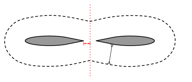
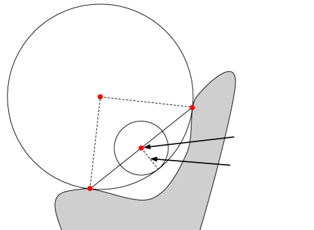
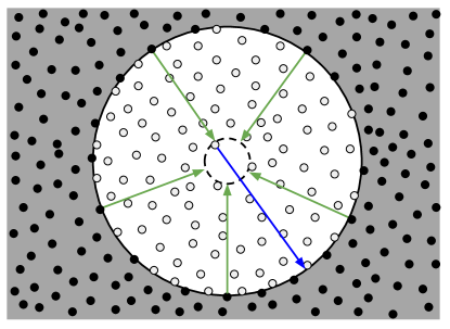
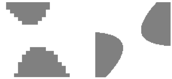
To see that the -convexity and the reach of a set are indeed distinct notions for general subsets of , Figure 1 provides an example of a closed set for which . Consider also the following remark.
Remark 1.
Any closed subset of contained in a -dimensional affine linear subspace is -convex for all . This is easy to see since the complement of the set in the -dimensional affine linear subspace is open, and is the union of open -balls of radius less than . Each -ball can be expressed as the intersection of the affine linear subspace with an open ball of radius in ; therefore, the closed subset in question can be expressed as the complement of a union of open balls of radius and is hence -convex.
Recently, a counterexample to Borsuk’s conjecture that -convex sets are locally contractible, was published in [24]. The conjecture is easily seen to be false by mapping a closed set in that is not locally contractible to a -dimensional hyperplane in under an isometry.
Here, we provide some corollaries to Theorem 1 that provide alternative sets of sufficient conditions for the equality of the reach and the -convexity. The first applies to sets in Serra’s regular model [50, p. 144].
Corollary 1.
Let be non-empty, compact, and path-connected. If , then .
The proof of Corollary 1, which relies heavily on Theorem 1 in [53], is postponed to Section 5. Likewise, we prove the following result in Section 5.
Corollary 2.
Let be a closed set in and let . Then .
2.2.2 The -reach
We show in Theorem 2 below, that the reach of a set can be formulated in terms of pairs of points in the set, and the distance to the set from their midpoints. We define a parametrized version of the reach by restricting to pairs of points whose midpoints are sufficiently far from the set. The so-called -reach is constructed from the following family of functions.
Definition 5 (Spherical cap geometry).
Define for and ,
| (4) |
and its inverse for ,
| (5) |
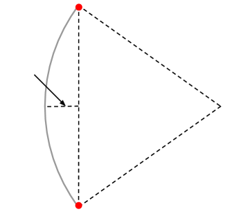
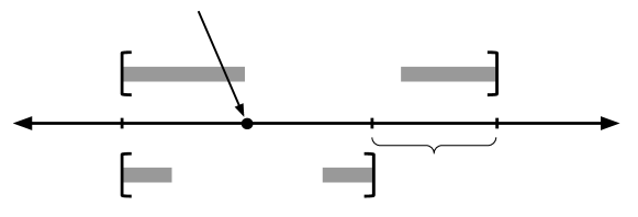
See Figure 3 for a geometric interpretation of the function in (4) and its inverse in (5). Evidently from the figure, this function is derived from the height of a spherical cap; it is written about in [7, 6, 10, 16, 37] in reference to the reach.
Definition 6 (The -reach).
By restricting to pairs of points in Figure 4 that yield , the -reach of is the largest lower bound of the resulting values of . If one does not restrict the size of (i.e., for ), then this largest lower bound is precisely . This is formalized by the following theorem.
Theorem 2.
Let be closed in . The map for is non-decreasing; moreover,
| (6) |
Proof: [Proof of Theorem 2] The non-decreasing property is seen immediately via the inclusion
for all satisfying .
Now, we start by proving the second equality in (6). The proof is largely supplied by Lemma 1 of [16] which provides
| (7) |
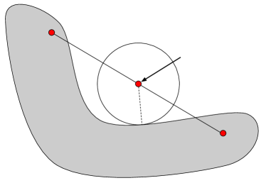
for all , since is non-increasing in . What remains to show is that is the largest lower bound in (7); i.e., if then there exist such that exceeds the right-hand side of (7). Let and let . By the definition of (Definition 2), and such that . Since the interior of does not intersect , we have
(see Figure 5) and
This proves that .
Finally, we show the first equality in (6). The non-decreasing property gives . Now, it suffices to show the reverse inequality. For any , there exists satisfying
Any such pair must satisfy , and so for , it holds that . Thus, .
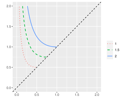
Remark 2.
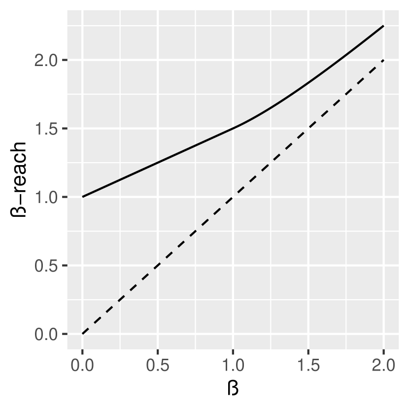
For any and , one has (see Figure 2). Thus, for any closed set and ,
Intuitively, this means that the -reach excludes small, reach-limiting features of the set that have scale less than .
The values of for which are the distances from the critical points of the generalized gradient function [18] to the set .
Remark 3.
Other generalizations of the reach are constructed similarly to the -reach, in that they formulate the reach as an infimum or supremum over some set, and add or remove elements in the set using some real parameter (in our case, ). For example, [16, Theorem 1] expresses the reach of a set as the supremum over a subset of that satisfies a certain condition relating to . By “continuously” weakening the condition with a parameter , the authors in [1] introduce the spherical distortion radius as the supremum of the larger subset of satisfying the weaker condition parametrized by . The spherical distortion radius is identified with the reach for . In an earlier work, [18] introduces the -reach by considering the shortest distance from an element in the set to the -medial axis, a filtered version of the medial axis by considering regions where the generalized gradient function [41] is less than some . The -reach, the -reach, and the spherical distortion radius, are all generalizations of the reach that exclude “small-scale” features as decided by the corresponding parameter , , or .
One significant advantage of the -reach is its computability for high-dimensional point cloud data (see Section 3.3). In this setting, the formulation of the reach in terms of the -reach for can also be used to construct an upper bound for the reach of any compact (see Section 3.2).
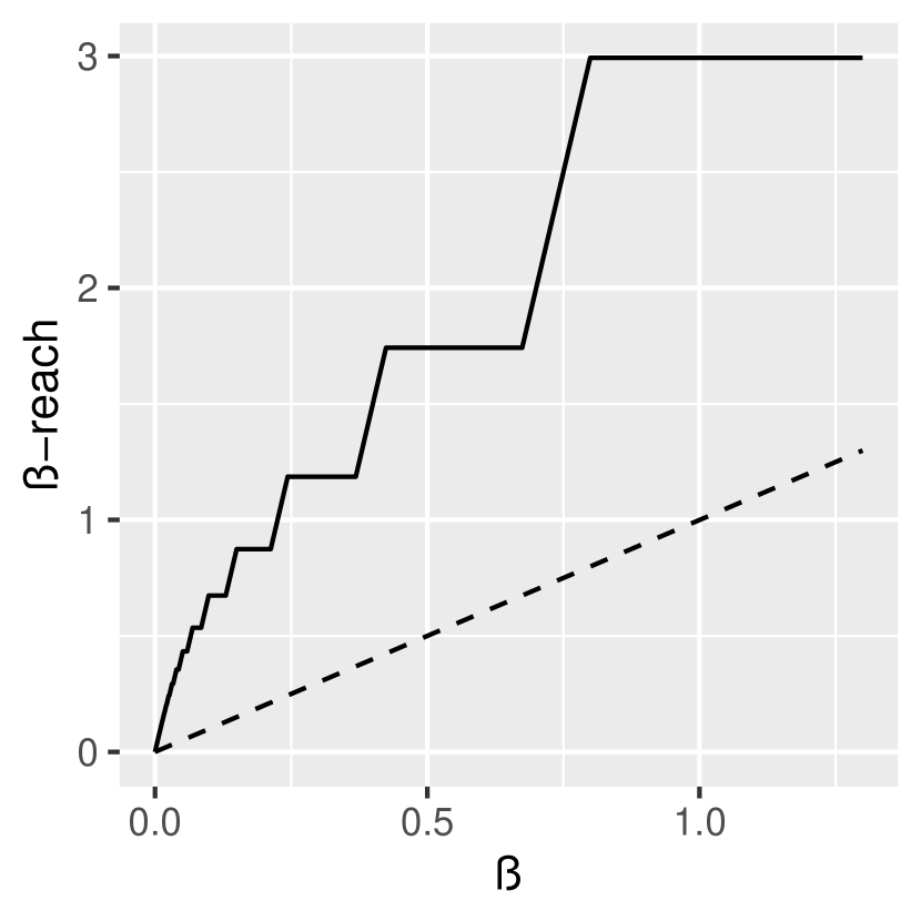
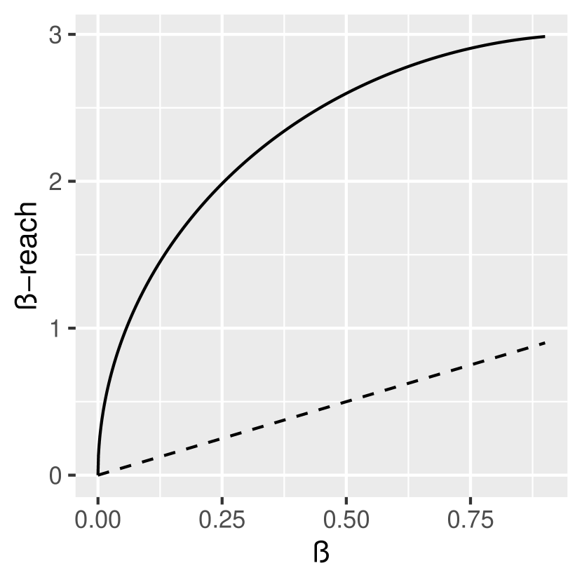
For a closed set , one can study the map for , which we refer to as the -reach profile of the set . We will see in Section 3 that a set’s -reach profile provides pertinent information regarding the estimation of the reach from point cloud data, especially through its first-order approximation at .


Some exemplary sets and their -reach profiles are considered in the several examples that follow.
Example 1 (The -reach of a corner).
For two line segments in with ends joined by an angle , the -reach of their union is , for sufficiently small . See Figure 6 for an illustration.
Example 2 (The -reach of an arc).
The -reach of a circular arc of angle at most is equal to the radius of the arc, for sufficiently small .
Example 3 (The -reach of a bottleneck structure).
If the reach of a set is determined by a bottleneck structure like those described in [2], then for . This is the case, for example, when is a finite set of points in .
Example 4 (The -reach of a -smooth curve).
Let be a -smooth function with . Suppose that the graph of the function defined by obtains its maximal curvature at . Then, the graph satisfies
| (8) |
and
| (9) |
for sufficiently small . Justifications for Equations (8) and (9) are provided at the end of Section 5. Figure 7 depicts a special case of this example with .
3 Methods for point cloud data
In practice, one might be interested in identifying bounds on the reach and -convexity of a set given a discrete set of points that are known to reside in . The goal of this section is to provide computational methods for bounding the reach and the -convexity from above, and producing diagnostics for possible approximations. The three main settings that we consider are:
-
(a)
One has access to a point cloud that extends over in the sense that can be covered by balls of fixed radius centered at each point. Moreover, one knows the partition of the points that lie in , and those that lie in . See section 3.1 for a treatment of this setting.
-
(b)
One has access to a set of points for which it is known that can be covered by balls of fixed radius centered at each point. Here, is known. See section 3.2.
-
(c)
The set is a submanifold of of dimension . One has access to a set of points that is known to be contained in . See section 3.3.
The mathematical results that we present in this section hold in arbitrary dimension . Nevertheless, the computational complexity of the method described in Section 3.1 for setting (a) increases quite drastically as higher dimensions are considered.
For the method that we present for setting (b) described in Section 3.2, its computation time depends on the ambient dimension only through the computation of distances in , which is linear in . The algorithm is largely dependent on the number of points used, which may be large in high dimension to ensure small .
The computational complexity of visualizing the -reach profile of the manifold in setting (c) is also linear in the dimension of the ambient space, and so the algorithm that we describe in Section 3.3 can adapt to large values of . Contrast this with existing methods that aim to approximate the reach by first approximating the medial axis [33, 21, 18, 36, 35, 42], where in high dimension, accessing the medial axis becomes computationally challenging. The relationship between , , , and our method’s performance is elaborated on in Remark 10 in Section 3.3.
3.1 An upper bound for the -convexity of a set
In this section, we introduce a method for identifying when sets are not -convex, for , with a true negative rate of 100%. That is, given a set that is observed over some grid of points (possibly lacking structure), we show how to correctly identify for which values of the set is certainly not -convex. The smallest of these values of provides an upper bound for , and by Equation (2), an upper bound for . Moreover, if the sampling becomes dense in , we show that this upper bound converges to .
Here, we define operations analogous to dilation and erosion, for discrete sets of points.
Definition 7.
Let be a point cloud in , i.e., a countable subset of . For a set , we make a slight abuse of notation and denote for ,
Remark 4.
We emphasize that for a point cloud , a subset , and a real number , Definition 7 implies that . Contrast this with the set , which is not contained in for .
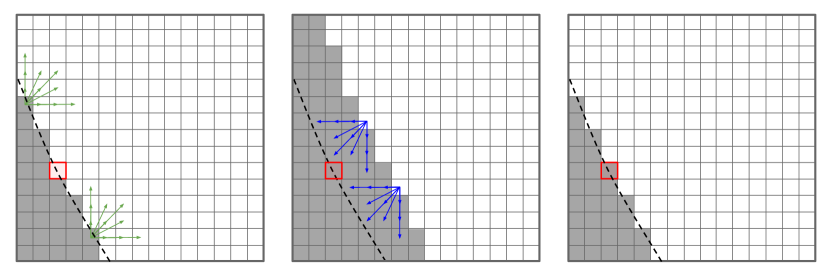
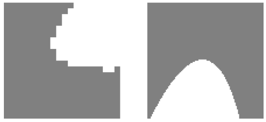
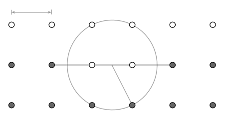
Let us illustrate the operations in Definition 7 using the example in Figure 8. The set occupies the bottom left corner of the domain, just until the dashed line. When sampled on a square lattice , one obtains the image in panel (a); each pixel is centered on a point in , and grey if the point lies in . Dilating the grey pixels by , one obtains the grey pixels in panel (b), . If one then erodes by (equivalent to dilating by and taking complements), one obtains the grey pixels in panel (c), . Notice, however, that there is a point in that is not in . This might be surprising since we chose a set such that . This illustration shows that naively testing for -convexity using the discrete dilation and erosion operations mistakenly classifies sets as not -convex when indeed they are.
The following theorem shows how to correctly identify sets as not being -convex, and gives an upper bound for the -convexity of a set that is tight in some sense.
Theorem 3.
For , let be a point cloud in , and suppose that
| (10) |
is finite. Let be a compact subset of , and for , define and the corresponding bound,
| (11) |
It holds that
| (12) |
Moreover, if and as , then
| (13) |
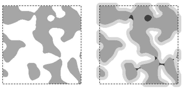
Theorem 3 provides a method for correctly identifying which subsets of are not -convex. If a dilation of the the discretization by followed by an erosion of produces a set that is not contained in , then . See Figure 9 for an example of a set for which . The precise regions where -convexity does not hold are highlighted by the method.
Remark 5.
Note that in (11) can be computed using entirely available information, since in (10) is a feature of the point cloud and not of the unknown set . In particular, there is no need to estimate for the construction of . A binary search algorithm, along with the discrete dilation operations in Definition 7, are sufficient for the numerical calculation of .
Remark 6.
The requirement that extends over all of (see Equation (10)) allows for a mathematical simplification and is not needed in practice. In real applications, one only requires that for some compact that contains . In the case where is lower dimensional than the embedding space , one can add any finite number of points uniformly distributed on to , and they will almost surely not belong to .
The proof of Theorem 3 is quite technical, and so we postpone it to Section 5. Nevertheless, Figure 10 provides an intuitive illustration that helps understand Equation (12). This is an example of a worst-case scenario, in that a dilation of by any more than results in all of being consumed. The dilation radius is maximal in the sense that, by dilating any less, there is guaranteed to be at least one element of that is not in the dilation. The distance between this one remaining element of and the other points in might be anywhere up to , where is the dilation radius. Therefore, an erosion by at least is necessary to guarantee that the resulting set is a subset of . In this sense, the bound in (12) is tight.
The following result from [49], while interesting on its own, is instrumental in the proof of Equation (13).
Proposition 1 (Lemma 8.3 in [49]).
Let and let be a closed set satisfying . The set contains an open subset of .
The relationship between Proposition 1 and Equation (13) is that, for , as the point cloud becomes more dense in , the open subset in fills with points that remain in for sufficiently small. Thus,
and since is arbitrary, the limit is at most . Equality then holds by Equation (12). The full proof of Theorem 3 and an alternative proof of Proposition 1 are provided in Section 5.
Remark 7.
Equation (13) is provided without a rate of convergence. This is due to the fact that Proposition 1 provides no guarantees on the size of the open subset that can be found in for . To provide a rate of convergence, a deeper analysis is needed to understand the rate at which the size of the largest open ball in decreases as . Conversely, the bound that we construct for the reach in Section 3.2 converges to the reach at a known rate (see Theorem 4 below).
3.2 An upper bound for the reach of a set
We have already seen that in (11) is an upper bound for the reach by Equations (2) and (12). In this section, we introduce another computable bound for the reach based on the expression for the -reach in Definition 6. The context in which one can apply this bound was introduced as setting (b) at the start of Section 3: a countable set of points is known to be included in a compact set , and its Hausdorff distance to is known to be at most .
A very weak regularity condition is imposed on the set in terms of its -reach profile near 0; it is used to prove the rate at which our upper bound converges to as in the Hausdorff metric.
Assumption 1.
Suppose that the set is compact, and that there exists such that the map for is either constant or strictly increasing on . In addition, suppose that
| (14) |
exists and is finite.
Assumption 1 is imposed on the -reach of , as opposed to the regularity of , since the -reach lends very naturally to the proof of Theorem 4. Moreover, Assumption 1 allows for most compact sets in , excluding some pathological counterexamples such as hypothetical sets admitting the -reach profiles in Figure 11. Assumption 1 is seen to hold in all of Examples 1 through 4 in Section 2.2.2.
Theorem 4.
Let be closed. For each , let be a countable subset of . Suppose that in the Hausdorff metric. i.e., there is a sequence in tending to 0 as such that for all . For each , define the corresponding bound on by
| (15) | ||||
where is defined in (4). Then,
| (16) |
for . Furthermore, if satisfies Assumption 1 and is not convex, then there exists such that
| (17) |
for all , where is defined as in (14).
Proof: [Proof of Theorem 4] We begin by showing (16) in the case where is not convex (for convex, the result is trivial since [39]). Suppose that for some fixed , we have . We write,
| (18) |
The equality in (3.2) is an application of Definition 6, and the inequality holds since the infimum is taken over a smaller subset. For any , there exists a projection of onto , namely , satisfying
By the triangle inequality and the fact that ,
Rearranging gives,
| (19) |
Since is non-increasing, the rightmost expression in (3.2) cannot decrease when is replaced by . Thus,
where the latter equality is an application of Theorem 2.
Now, we proceed to show (17). Recall the equality in (3.2), and split the analysis into two cases.
- Case 1:
-
There exists such that and .
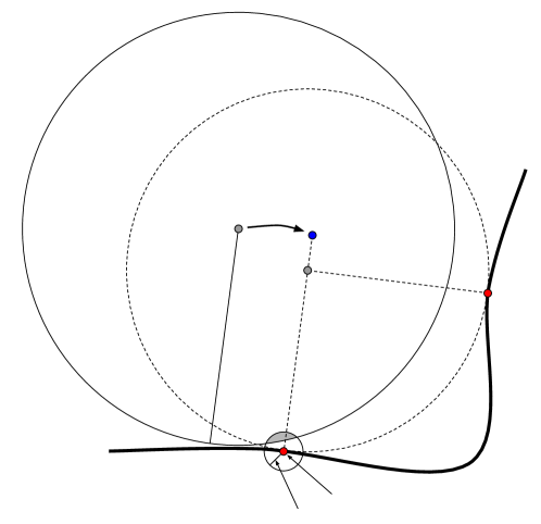
For this pair there exists satisfying . This implies(20) Equation (20) tells us that the two midpoints are close, and so their distances to cannot differ by more than the distance between them. i.e.,
Since Equation (19) holds for , and , we also have
(21) by the triangle inequality (see Figure 12).
Now, suppose that is sufficiently large such that . Then, by (21), and so
(22) The second inequality in (Case 1:) holds since , and the final inequality holds by Equation (21).
Recall that . The difference between this and the final expression in (Case 1:) is of the order , which is stronger than required.
- Case 2:
-
for all distinct .
By Assumption 1, for all sufficiently large , the function is strictly increasing for in a neighbourhood of . For each of these values of , definewhich is compact by Assumption 1, and the continuous map by
Remark that , and so there is an element for which
By Definition 6, for . The -reach profile of is thus constant on the interval by Theorem 2, but by Assumption 1, any such interval must have length 0. Therefore,
Remark 8.
The split of the proof of Theorem 4 into two cases is natural in the context of reach estimation. Recall Theorem 3.4 in [2]: For a compact set with , there is either a bottleneck structure (two distinct points such that ) or an arc-length parametrized geodesic of with curvature . The convergence rate developed in Case 1 applies to sets whose reach is decided by a bottleneck structure, and that of Case 2 applies to sets whose reach is decided by a region of high curvature.
Remark 9.
In [1], the authors provide a minimax optimal rates of convergence for statistical estimators of the reach. The authors proceed by assuming that is a -smooth manifold without boundary, with . The minimax rates in [1, Theorem 6.6] are expressed in terms of , the number of continuous derivatives of the underlying manifold.
It is not surprising that our bound on the reach—for sets satisfying the very general Assumption 1—does not converge to the reach at the optimal rates given in [1]. Nevertheless, we do observe a similar phenomenon in that the rate of convergence derived for a set whose reach is determined by a bottleneck structure ( in Case 1 in the proof of Theorem 4) is faster than the rate when the reach is determined by a region of high curvature ( in Case 2).
3.3 The -reach profiles of high-dimensional point clouds
Here, we tackle the problem of approximating the reach of smooth manifolds of low dimension embedded in high-dimensional Euclidean space. As discussed in the introduction, this setting is the focus of many works. Given a -smooth manifold of dimension , we suppose that one has access to a set of points from which one would like to infer .
Recall from Definition 6 that the -reach of a point cloud is easily computable, and the computation time does not heavily depend on the dimension of the ambient space. The -reach profile of a point cloud can be obtained by considering pairs of points in the point cloud and computing the distance from their midpoint to the closest neighbour in the point cloud. For a fixed number of points, the computation time for calculating the exact -reach profile of the point-cloud scales linearly in . Of course, the -reach profile of is not identical to that of , however, we argue here that it provides a good approximation for the values of away from 0.
Recall that the bounds developed in Sections 3.1 and 3.2 are for subsets of that possibly have positive -volume. This means that a point cloud contained in a set can recede a distance from the topological boundary of . Thus, the distance from a point in to can be up to shorter than the distance to the nearest point in . Conversely, for a smooth manifold embedded in , projection of an element onto is along a vector normal to at the projection in . Thus, the distance from to its nearest point in is more similar to the length of the projection vector, so in this setting, the bounds constructed previously are overly robust. Moreover, existing algorithms for computing a mesh from point cloud data can be leveraged to improve quality of the estimate of the distance to the nearest point in , thus improving the estimate of the -reach.
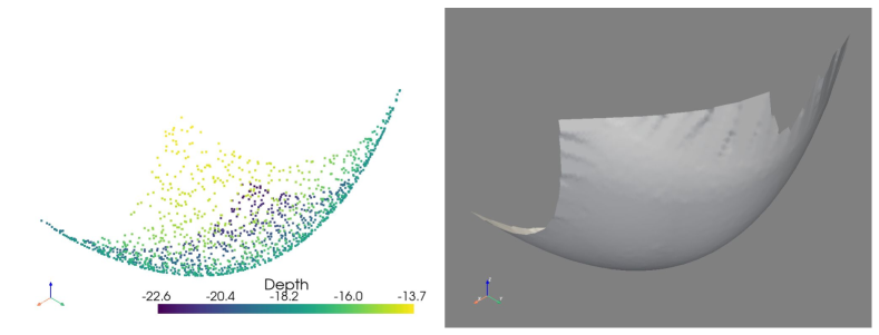
Example 5 (3-dimensional point cloud on a 2-dimensional manifold).
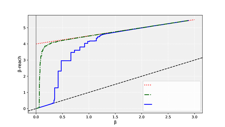
Let be a section of a two-dimensional paraboloid, where its reach is decided by a point of maximal curvature at the vertex (). Let be a realization of points uniformly distributed on shown in Figure 13 (a). Using the Python library pyvista [51], we construct a mesh over the point cloud (see Figure 13 (b)). This allows for an improved approximation of the -reach profile of ,
| (23) | ||||
The -reach of can be computed exactly as , for between 0 and some positive constant. As seen in Figure 14, this is well approximated by for , and by for ; both approximations are efficiently computable from the point cloud .
To estimate from the -reach profiles in Example 5, one can perform a linear regression on , for in the range where the curve appears linear, and estimate the reach as the model intercept.
Although the manifold in Example 5 is derived from a simple paraboloid, this example is representative of other two-dimensional manifolds whose reach is determined by a region of high curvature. The difference might be that the linear term in the first order approximation of the -reach profile at does not have a coefficent of 1/2 (see Example 4).
The following two examples emphasize the applicability of this method in higher dimensions.
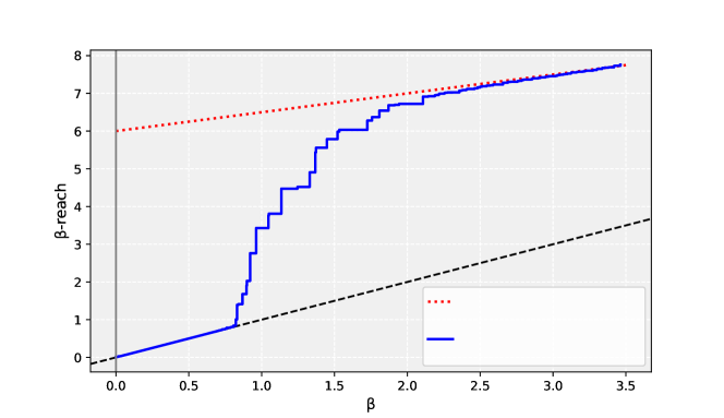
Example 6 (-dimensional point cloud on a 3-dimensional manifold).
Let , and let be a section of the three-dimensional paraboloid defined by , such that its reach is decided by a point of maximal curvature at the origin. It can be shown that , for between 0 and some positive threshold.
Let be a realization of points, uniformly distributed on . The Python package pyvista does not currently have methods for computing meshes in dimension higher than 3, so in this example, we do not compute in (23). Mesh generation in higher dimension is itself an active field of research [17, 15, 38]. Nonetheless, we plot the exact -reach profile of in Figure 15.
Remark 10.
The dimension of the ambient space in Example 6 does not affect the shape of the -reach profile of the point cloud , computed purely in terms of distances between the points, and distances to midpoints. These distances are preserved under isometries to higher dimensional spaces. However, the number of points in plays a role in the shape of the -reach profile through the Hausdorff distance between and the underlying manifold . The exact relationship between the number of points in and the Hausdorff distance cannot be made precise with no prior knowledge of how the points are distributed on —which also plays a role in the shape of the -reach profile of . Nonetheless, the dimension of determines to a large extent the number of points needed to ensure that is less than a given tolerance.
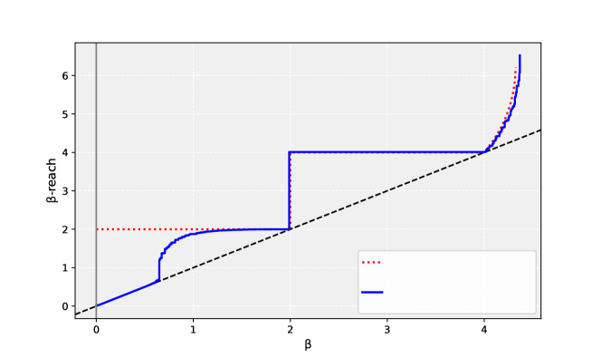
Example 7 (Two 3-dimensional hyperspheres).
Let , and let be the union of two three-dimensional hyperspheres of radius 2 whose centers are 12 units apart. Let be a realization of points uniformly distributed on . The -reach profiles of and a realization of are shown in Figure 16.
Example 7 highlights a few nice features of the -reach profile. That is, it adapts very well to situations where the reach is determined by a bottleneck structure, as is the case for a hypersphere. For , the -reach is no longer determined by the radius of the hypersphere, but by half the distance between the surfaces of the spheres (in this case, units). Thus, the -reach profile also provides information about the large scale features of the data. Notably, it gives the scales at which it becomes possible to distinguish these features from one another.
4 Numerical studies
In this section, we test the methods for bounding the reach and -convexity introduced in Section 3 against numerical data. First, in Section 4.1, we study the performance of our methods on real data. Then, in Section 4.2, we test the convergence results in Theorems 3 and 4.
4.1 Aircraft data
The real data in Example 8, below, is studied using the tools developed in this document. After a short description of the data, we perform several analyses using the tools developed in Section 3.
Example 8 (Aircraft data).
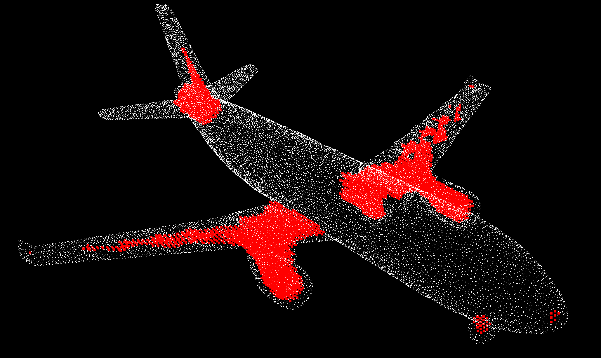
[8] provides a point cloud dataset that is sampled over the surface of a commercial aircraft (the white points in Figure 17 (a)). The diameter of the raw point cloud data (which corresponds to the length of the plane) is 0.749 units. Denote the surface of the aircraft by and the approximating point cloud by .
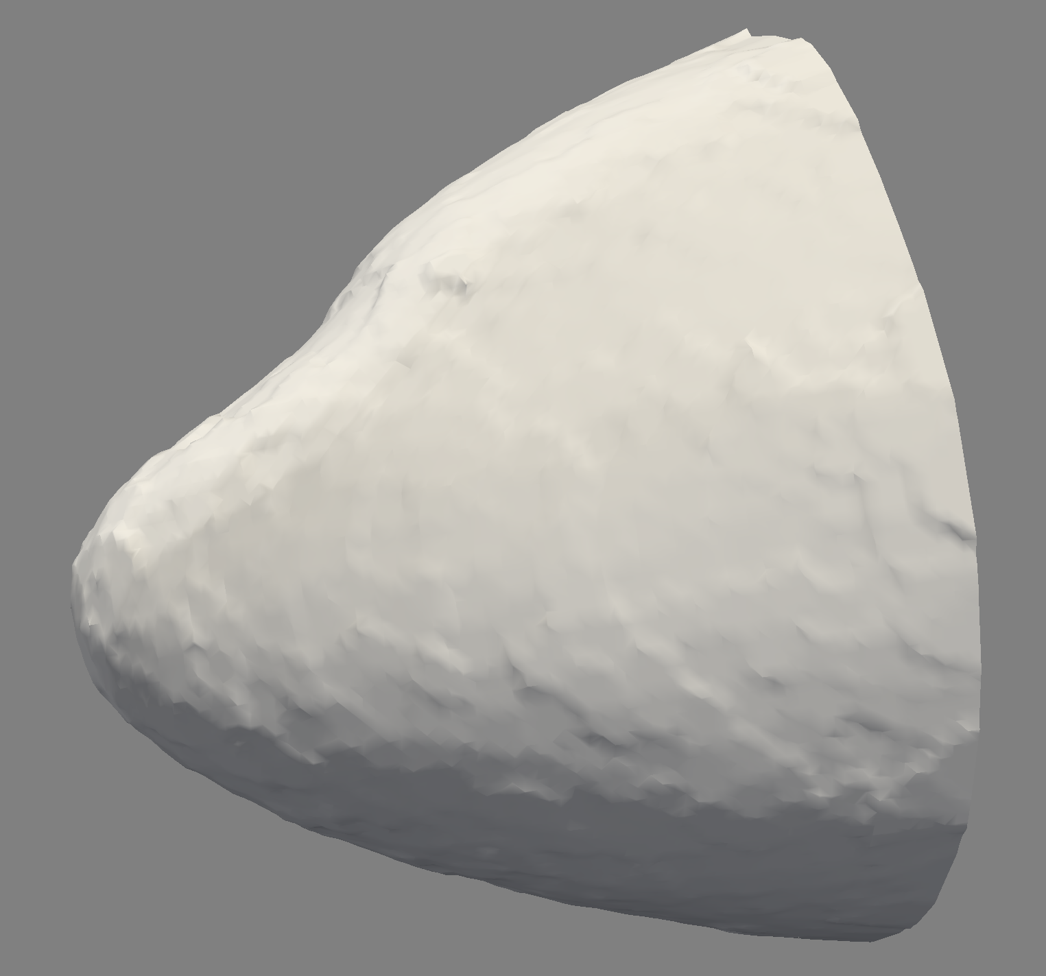
We are also interested in the nose of the aircraft, , the surface of the first 0.056 length units of the aircraft. A two-dimensional mesh approximating is shown in Figure 17 (b).
It is possible that in an engineering practice, one may want to identify which regions of a point cloud are not -convex for a predefined value of . Panel (a) of Figure 17 highlights in red the regions of the plane that are certainly not -convex for the choice of .
The surface of the plane is known to be two-dimensional, and so a cubic lattice of points with lattice spacing superimposed over will almost surely not intersect . The discrete dilation and erosion operations in Definition 7 are well defined using the larger point cloud . The red points in Figure 17 (a) are the elements of the discrete set , with . Since this set is not empty, one has that is a proper subset of . In addition, by (2), one has conclusive evidence that .
This example illustrates that, with this method, one can identify the regions responsible for limiting the -convexity (and thus the reach), with a test specificity of 100%. One can improve the sensitivity of the test by decreasing the lattice spacing . Then, other regions that are not -convex (such as the interiors of the horizontal and vertical stabilizers) would be identified as such.
Remark that the nose of the plane is marked in red, due of course to a region of high curvature. By considering only the smooth manifold in Example 8, corresponding to the nose of the plane, we can approximate the -reach profile of by in Definition 6, or by in Equation (23).
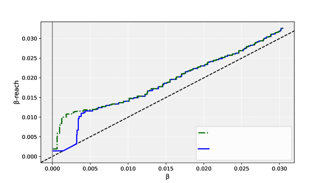
The resulting -reach profiles are shown in Figure 18. From the figure, the reach is clearly seen to be much smaller than as indicated by the -convexity experiment. Assuming that the -reach profile of maintains a constant slope near 0 as seen before in Figure 14, the approximation can be read from Figure 18.
There are two main issues with using the reach bound in (15) on the aircraft data in Example 8. First, it is expected to produce a large overestimate of since is a smooth manifold (see the discussion in Section 3.3). In addition, it is impossible to know the Hausdorff distance beween and its approximating point cloud . Nevertheless, one can obtain a good approximation by considering the persistence diagram of growing balls centered at the points in . The largest of the death-times of the topological features corresponds to the smallest radius for which the union of balls is homotopic to a point. This is likely to corespond closely to the Hausdorff distance , and is thus a good choice for in (15). The persistence diagram, generated from the Python module ripser [9], gives that the largest death-time is . From this, one calculates
4.2 Numerical convergence of reach and -convexity bounds
In stochastic geometry literature, the excursion set of a random field is the subset of its domain on which the random field surpasses a predefined threshold (see [5] for a comprehensive reference). The set in Figure 9, for example, is one realization of the excursion set of a stationary, isotropic Gaussian random field sampled on a square lattice.
The following two examples are meant to imitate the discretized excursion set of continuous random fields on square lattices (see, e.g., [29, 28, 12]). A key feature of both examples, is that the reach and -convexity of the sets are known, and so we can study the convergence of the bounds in Theorems 3 and 4 as the grid of sampling points becomes dense in . Each example illustrates one of the two cases mentioned in Remark 8 concerning the relationship between the reach, regions of high curvature, and bottleneck structures.
Example 9 (Reach determined by curvature).
Let . It is easy to check that . Moreover, the reach is determined by a point of maximal curvature at .
Let be a sequence of square lattices over with lattice spacing , and independent, uniformly random position and orientation. For , let be the set sampled on . Figure 19 depicts square subsets of realizations of and shown as binary images.
Example 10 (Reach determined by a bottleneck structure).
Let . One has , which is half the distance between its two connected components.
Remark 11.
The choice to use sets with a reach of 1 in Examples 9 and 10 does not limit their generality. The importance lies in the scale of the sampling lattice relative to the reach, and the ratio of the two tends to 0 as in both examples.
The following observation makes the gernerality of these examples even clearer: to consider the lattice of sampling points at various scales and orientations is equivalent to considering a fixed lattice and various scales and orientations of the underlying sets and .
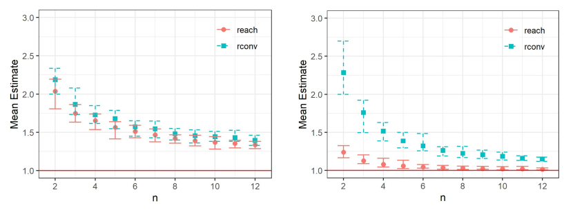
For each , we compute 50 independent realizations of and 50 independent realizations of . For each of the resulting discrete sets, we compute the bounds of -convexity and reach in (11) and (15) respectively. The means of the bounds are plotted in Figure 21 with empirical 95% confidence intervals. Panels (a) and (b) correspond to the results for the replications of and respectively.
For the -convexity bound, is chosen since , for .
For the reach bound, we set for reasons that are more complicated. Even though this choice of leads to , or with positive probability, it is sufficient for the result of Theorem 4 in this case. We provide Figure 22 for some intuition, but a formal proof is omitted.
A linear regression on the log-log plot of the sample means of the data in Figure 21 (a) shows that
These empirical convergence rates — for the bound on and for the bound on — are both slightly faster than the predicted rate of established in (17) for the bound on the reach. Since the reach of is determined by a region of maximal curvature, the convergence rate is governed by the analysis in Case 2 in the proof of Theorem 4.
5 Proofs and technical results
Proof: [Proof of Theorem 1] We begin by showing (2). Suppose that . By Lemma 1, , so it suffices to show that . Let . If , then clearly, . If , then by Federer, [39, Corollary 4.9],
and so , which proves (2). What remains to be shown is that if is -smooth and -dimensional, then . This inequality is shown via proof by contradiction. Suppose that
-
(i)
and
-
(ii)
.
By (i), there exists with no unique point in closest to . In particular, since is closed, there exists two non-identical points such that . Let be the unit normal vector to at , pointing towards . Since is a limit point of , one has for all . By (ii), , and so for all , there exists such that
-
(iii)
and
-
(iv)
.
The boundary is -smooth at , so it is easily checked that for close to 0, the locations that satisfy both (iii) and (iv) are necessarily contained in a small neighbourhood around (see Figure 23). That is, there exists a mapping that tends to 0 as , such that if and satisfy (iii) and (iv), then . Note that since . Choose such that . Then for any ,
This contradicts (iv).
Lemma 2.
Let be an open set in , and let . Then,
Proof: [Proof of Lemma 2] By Lemma 1, item (b), . Note also that is open. Suppose that . Then is an open subset of that contains all of the interior points of . Therefore, .
Lemma 3.
Let be closed. It holds that
Proof: [Proof of Lemma 3] By Lemma 2 and item (a) in Lemma 1, . Therefore, . Now we show the reverse inequality. Let satisfy . By Proposition 1, contains a ball of radius for some . Now, let . Note that , and so by Lemma 1, , which contains the ball of radius . Now, eroding by preserves a ball of radius . That is, contains a ball of radius that does not intersect , and so which implies the desired by Lemma 1, item (a).
Proof: [Proof of Corollary 1] If , then by Theorem 1, and we are done. Now assume and , then by Lemma 3, there exists such that for all . Theorem 1 in [53] states that is -dimensional and -smooth, which implies Equation 3 in our Theorem 1.
Proof: [Proof of Corollary 2] By Theorem 1, the statement holds if is -smooth and -dimensional. Otherwise, if there is indeed a point on the boundary of that does not have a continuous derivative, then is an intersection point of two distinct -spheres centered in of radius . In other words, is at cusp that points inwards towards the interior of , making .
Remark 12.
Lemma 4.
For closed and , it holds that
| (24) |
Proof: [Proof of Lemma 4] By manipulating the expressions in Definition 1, one obtains
| (25) |
which reads: the elements of are the such that is not contained in any closed ball of radius that does not intersect . This statement is equivalent to: if and only if there exists a closed ball of radius that contains but does not intersect . Thus, we have shown that is equal to the complement of the RHS of (24), which proves the desired result.
Proof: [Proof of Proposition 1] Let and fix . Since is closed, there is an open neighbourhood containing that does not intersect . Choose such that . There exists a sufficiently small such that for every , there exists an that satisfies . Since , one has that contains an element of by Lemma 4. By inclusion, contains a point in as well.
Let . We have shown that is in the right-hand side of (24), since, for all , one has by the triangle inequality, and so by previous arguments, contains an element of . Therefore, by Lemma 4, . But is not in since . Therefore, and so .
Proof: [Proof of Theorem 3] We begin by showing (12). Let and fix . If , then (12) holds trivially. Now, let be such that so that . We aim to show that . Indeed, by the -convexity of , there exists such that . In addition, , so there exists such that . Therefore, by the triangle inequality, , which implies . Thus, as desired.
Now, to prove (13), first fix . To simplify notation, let . By Proposition 1, there exists an open subset that contains a closed ball of radius for sufficiently large . Let . The point cloud is sufficiently dense such that there exists . Importantly, this implies that . By Lemma 1, for all , we have , and therefore . Notice that , which implies and thus . Summarizing, we have shown that there is a point in that is not in . By the change of variables , it follows that for all , which implies . Sending yields , and since was chosen freely, . This result, along with (12), gives the convergence in (13).
Justification for Equations (8) and (9).
The reach of is equal to the inverse of the curvature of at [2, Theorem 3.4]. Equation (8) holds since the curvature of at is .
Now we show (9). Without loss of generality, suppose . For in a neighbourhood of 0, consider the symmetric points and in , and remark that
| (26) |
since . We claim without proof that for all satisfying , it holds that . In the language of the -reach, this is equivalent to
| (27) |
There is a such that has an inverse on , and so for , choose such that . Remark that
by Taylor’s theorem. Plugging into (26) and applying (27), one obtains (9).
References
- Aamari et al., [2022] Aamari, E., Berenfeld, C., and Levrard, C. (2022). Optimal reach estimation and metric learning. Preprint arXiv:2207.06074, pages 1–47.
- Aamari et al., [2019] Aamari, E., Kim, J., Chazal, F., Michel, B., Rinaldo, A., and Wasserman, L. (2019). Estimating the reach of a manifold. Electronic Journal of Statistics, 13(1):1359–1399.
- Aamari and Levrard, [2019] Aamari, E. and Levrard, C. (2019). Nonasymptotic rates for manifold, tangent space and curvature estimation. The Annals of Statistics, 47(1):177–204.
- Aaron et al., [2022] Aaron, C., Cholaquidis, A., and Fraiman, R. (2022). Estimation of surface area. Electronic Journal of Statistics, 16(2):3751–3788.
- Adler and Taylor, [2007] Adler, R. J. and Taylor, J. E. (2007). Random fields and geometry. Springer Monographs in Mathematics. Springer, New York.
- Attali and Lieutier, [2015] Attali, D. and Lieutier, A. (2015). Geometry-driven collapses for converting a Čech complex into a triangulation of a nicely triangulable shape. Discrete & Computational Geometry, 54:798–825.
- Attali et al., [2013] Attali, D., Lieutier, A., and Salinas, D. (2013). Vietoris–rips complexes also provide topologically correct reconstructions of sampled shapes. Computational Geometry, 46(4):448–465. 27th Annual Symposium on Computational Geometry (SoCG 2011).
- Baorui et al., [2022] Baorui, M., Yu-Shen, L., Matthias, Z., and Zhizhong, H. (2022). Surface reconstruction from point clouds by learning predictive context priors. In Proceedings of the IEEE/CVF Conference on Computer Vision and Pattern Recognition (CVPR).
- Bauer, [2021] Bauer, U. (2021). Ripser: efficient computation of Vietoris-Rips persistence barcodes. J. Appl. Comput. Topol., 5(3):391–423.
- Berenfeld et al., [2022] Berenfeld, C., Harvey, J., Hoffmann, M., and Shankar, K. (2022). Estimating the Reach of a Manifold via its Convexity Defect Function. Discrete & Computational Geometry, 67:403–438.
- Berrendero et al., [2012] Berrendero, J. R., Cuevas, A., and Pateiro López, B. (2012). A multivariate uniformity test for the case of unknown support. Statistics and Computing, 22:259–271.
- Biermé and Desolneux, [2021] Biermé, H. and Desolneux, A. (2021). The effect of discretization on the mean geometry of a 2D random field. Annales Henri Lebesgue, 4:1295–1345.
- Biermé et al., [2019] Biermé, H., Di Bernardino, E., Duval, C., and Estrade, A. (2019). Lipschitz-Killing curvatures of excursion sets for two-dimensional random fields. Electronic Journal of Statistics, 13(1):536–581.
- Blum, [1967] Blum, H. (1967). A transformation for extracting new descriptions of shape. Models for the perception of speech and visual form, pages 362–380.
- Boissonnat et al., [2009] Boissonnat, J.-D., Devillers, O., and Hornus, S. (2009). Incremental construction of the delaunay triangulation and the delaunay graph in medium dimension. In Proceedings of the twenty-fifth annual symposium on Computational geometry. ACM.
- Boissonnat et al., [2019] Boissonnat, J.-D., Lieutier, A., and Wintraecken, M. (2019). The reach, metric distortion, geodesic convexity and the variation of tangent spaces. Journal of Applied and Computational Topology, 3(1):29–58.
- Boissonnat et al., [2008] Boissonnat, J.-D., Wormser, C., and Yvinec, M. (2008). Locally uniform anisotropic meshing. In Proceedings of the twenty-fourth annual symposium on Computational geometry. ACM.
- [18] Chazal, F., Cohen-Steiner, D., and Lieutier, A. (2009a). A Sampling Theory for Compact Sets in Euclidean Space. Discrete & Computational Geometry, 41:461–479.
- Chazal et al., [2007] Chazal, F., Cohen-Steiner, D., Lieutier, A., and Thibert, B. (2007). Shape Smoothing Using Double Offset. Proceedings - SPM 2007: ACM Symposium on Solid and Physical Modeling.
- [20] Chazal, F., Cohen-Steiner, D., Lieutier, A., and Thibert, B. (2009b). Stability of curvature measures. In Computer Graphics Forum, volume 28, pages 1485–1496. Wiley Online Library.
- [21] Chazal, F. and Lieutier, A. (2005a). The “-medial axis”. Graphical Models, 67(4):304–331.
- [22] Chazal, F. and Lieutier, A. (2005b). Weak feature size and persistent homology: Computing homology of solids in rn from noisy data samples. In Proceedings of the Twenty-First Annual Symposium on Computational Geometry, SCG ’05, pages 255––262, New York, NY, USA. Association for Computing Machinery.
- Chazal and Lieutier, [2008] Chazal, F. and Lieutier, A. (2008). Smooth manifold reconstruction from noisy and non-uniform approximation with guarantees. Computational Geometry, 40(2):156–170.
- Cholaquidis, [2023] Cholaquidis, A. (2023). A counter example on a borsuk conjecture. Applied General Topology, 24(1):125––128.
- Cholaquidis et al., [2022] Cholaquidis, A., Fraiman, R., and Moreno, L. (2022). Universally consistent estimation of the reach. Preprint arXiv:2110.12208v2, pages 1–15.
- Clarke and Wolenski, [1995] Clarke, F. and Wolenski, P. (1995). Proximal Smoothness and the Lower- Property. Journal of Convex Analysis, 2:117–144.
- Colesanti and Manselli, [2010] Colesanti, A. and Manselli, P. (2010). Geometric and isoperimetric properties of sets of positive reach in . Preprint, pages 1–15.
- [28] Cotsakis, R., Di Bernardino, E., and Duval, C. (2022a). Surface area and volume of excursion sets observed on point cloud based polytopic tessellations. Preprint arXiv:2209.10383.
- [29] Cotsakis, R., Di Bernardino, E., and Opitz, T. (2022b). On the perimeter estimation of pixelated excursion sets of 2D anisotropic random fields. Preprint hal-03582844v2, pages 1–28.
- Cuevas, [2009] Cuevas, A. (2009). Set estimation: Another bridge between statistics and geometry. BEIO, Boletín de Estadística e Investigación Operativa, 25:71–85.
- Cuevas et al., [2007] Cuevas, A., Fraiman, R., and Casal, A. (2007). A nonparametric approach to the estimation of lengths and surface areas. The Annals of Statistics, 35:1031–1051.
- Cuevas et al., [2012] Cuevas, A., Fraiman, R., and Pateiro-López, B. (2012). On Statistical Properties of Sets Fulfilling Rolling-Type Conditions. Advances in Applied Probability, 44(2):311–329.
- Cuevas et al., [2014] Cuevas, A., Llop, P., and Pateiro-López, B. (2014). On the estimation of the medial axis and inner parallel body. Journal of Multivariate Analysis, 129:171–185.
- Cuevas and Rodríguez-Casal, [2004] Cuevas, A. and Rodríguez-Casal, A. (2004). On Boundary Estimation. Advances in Applied Probability, 36(2):340–354.
- Dey and Sun, [2006] Dey, T. K. and Sun, J. (2006). Normal and feature approximations from noisy point clouds. In Arun-Kumar, S. and Garg, N., editors, FSTTCS 2006: Foundations of Software Technology and Theoretical Computer Science, pages 21–32, Berlin, Heidelberg. Springer Berlin Heidelberg.
- Dey and Zhao, [2003] Dey, T. K. and Zhao, W. (2003). Approximating the Medial Axis from the Voronoi Diagram with a Convergence Guarantee. Algorithmica, 38(1):179–200.
- Divol, [2021] Divol, V. (2021). Minimax adaptive estimation in manifold inference. Electronic Journal of Statistics, 15:5888–5932.
- Edelsbrunner, [2001] Edelsbrunner, H. (2001). Geometry and Topology for Mesh Generation. Cambridge University Press.
- Federer, [1959] Federer, H. (1959). Curvature measures. Transactions of the American Mathematical Society, 93(3):418–491.
- Kim et al., [2019] Kim, J., Shin, J., Chazal, F., Rinaldo, A., and Wasserman, L. (2019). Homotopy reconstruction via the cech complex and the vietoris-rips complex. Preprint arXiv:1903.06955.
- Lieutier, [2004] Lieutier, A. (2004). Any open bounded subset of has the same homotopy type as its medial axis. Computer-Aided Design, 36(11):1029–1046.
- Lieutier and Wintraecken, [2023] Lieutier, A. and Wintraecken, M. (2023). Hausdorff and gromov-hausdorff stable subsets of the medial axis. In Proceedings of the 55th Annual ACM Symposium on Theory of Computing, STOC 2023, pages 1768––1776, New York, NY, USA. Association for Computing Machinery.
- Mani-Levitska, [1993] Mani-Levitska, P. (1993). Characterizations of Convex Sets. In Handbook of Convex Geometry, pages 19–41. North-Holland.
- Niyogi et al., [2008] Niyogi, P., Smale, S., and Weinberger, S. (2008). Finding the Homology of Submanifolds with High Confidence from Random Samples. Discrete & Computational Geometry, 39:419–441.
- Pateiro López, [2008] Pateiro López, B. (2008). Set estimation under convexity type restrictions. Ph.D. thesis. [Link to thesis].
- Perkal, [1956] Perkal, J. (1956). Sur les ensembles -convexes. Colloquium Mathematicum, 4:1–10.
- Poliquin et al., [2000] Poliquin, R. A., Rockafellar, R. T., and Thibault, L. (2000). Local Differentiability of Distance Functions. Transactions of the American Mathematical Society, 352(11):5231–5249.
- Rataj and Zähle, [2019] Rataj, J. and Zähle, M. (2019). Sets with positive reach. In Curvature Measures of Singular Sets, pages 55–86. Springer.
- Rodríguez Casal and Saavedra-Nieves, [2016] Rodríguez Casal, A. and Saavedra-Nieves, P. (2016). A fully data-driven method for estimating the shape of a point cloud. ESAIM: Probability and Statistics, 20:332–348.
- Serra, [1984] Serra, J. (1984). Image Analysis and Mathematical Morphology. Academic Press.
- Sullivan and Kaszynski, [2019] Sullivan, C. and Kaszynski, A. (2019). PyVista: 3D plotting and mesh analysis through a streamlined interface for the Visualization Toolkit (VTK). Journal of Open Source Software, 4(37):1450.
- Thäle, [2008] Thäle, C. (2008). 50 years sets with positive reach—a survey. Surveys in Mathematics and its Applications, 3:123–165.
- Walther, [1999] Walther, G. (1999). On a Generalization of Blaschke’s Rolling Theorem and the Smoothing of Surfaces. Mathematical Methods in the Applied Sciences, 22:301–316.