Compound Batch Normalization for Long-tailed Image Classification

Abstract.

Significant progress has been made in learning image classification neural networks under long-tail data distribution using robust training algorithms such as data re-sampling, re-weighting, and margin adjustment. Those methods, however, ignore the impact of data imbalance on feature normalization. The dominance of majority classes (head classes) in estimating statistics and affine parameters causes internal covariate shifts within less-frequent categories to be overlooked. To alleviate this challenge, we propose a compound batch normalization method based on a Gaussian mixture. It can model the feature space more comprehensively and reduce the dominance of head classes. In addition, a moving average-based expectation maximization (EM) algorithm is employed to estimate the statistical parameters of multiple Gaussian distributions. However, the EM algorithm is sensitive to initialization and can easily become stuck in local minima where the multiple Gaussian components continue to focus on majority classes. To tackle this issue, we developed a dual-path learning framework that employs class-aware split feature normalization to diversify the estimated Gaussian distributions, allowing the Gaussian components to fit with training samples of less-frequent classes more comprehensively. Extensive experiments on commonly used datasets demonstrated that the proposed method outperforms existing methods on long-tailed image classification.

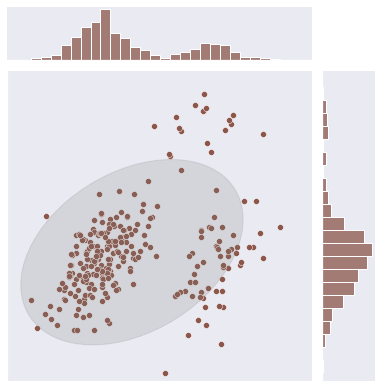
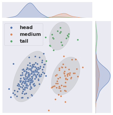
Figure 1. For an imbalanced training dataset, the conventional feature normalization (left), which leverages the single-modal Gaussian probability function to fit the feature space, is prone to overlook samples of tail classes. Adopting multiple Gaussian distributions to fit the features (right) can mitigate the above problem.

1. Introduction

Real-world image classification data usually exhibits an imbalanced distribution due to the natural scarcity of certain classes, industry barriers, and large data collection costs. The severely imbalanced data distribution causes substantial obstruction to the learning process, considering it is difficult to balance the classification performance of head and tail classes. The imbalanced learning problem attracts extensive research interests (Chawla et al., 2002; Cui et al., 2021; Samuel and Chechik, 2021). However, existing methods are incapable of deriving high accuracy on tail classes without hindering the performance of head classes or maintaining an efficient framework. This paper is targeted at learning with long-tailed training data while alleviating the above issues.

When learning deep convolutional neural networks (CNNs) with long-tailed samples, the optimization of network parameters is dominated by samples of head classes, which leads to relatively low performance for tail classes. Conventional solutions to the data imbalance problem is biasing the optimization process towards less frequent classes, such as class-balanced re-sampling (Chawla et al., 2002; Drummond et al., 2003), re-weighting (Huang et al., 2016; Wang et al., 2017), or classifier margin adjustment (Zhong et al., 2021; He et al., 2021). However, these data rebalancing methods hamper the learning of head classes by interfering the representation capacity of CNNs. A few works attempt to address this problem through ensembling multiple classifiers learned under diverse sampling strategies (Zhou et al., 2020) or adopting auxiliary classifiers to highlight the learning of tail classes (Xiang et al., 2020). However, such methods require increased network parameters and computation burden. Besides, the impact of data imbalance on feature representation learning can not be thoroughly alleviated since they still depend on data resampling or reweighting algorithms to manage multiple classifiers.

Batch normalization is a critical component for mitigating the internal covariate shift in the feedforward calculation process of CNNs (Ioffe and Szegedy, 2015). It can accelerate the optimization rate of network parameters and improve the generalization ability. Under the scenario of data imbalance, a single-modal Gaussian probability function can not fully model the feature space and is prone to overlook tail classes. Thus the conventional batch normalization can merely eliminate the global covariate shift, but neglect the internal covariate shift of tail classes. This harms the learning efficiency and generalization capacity on tail classes.

To address the above problem, we generalize the feature normalization by modeling the feature space with compound Gaussian distributions. As shown in Figure 1, the features of training samples are composed of several scattered clusters. For the purpose of fitting the features more comprehensively, we employ a compound set of mean and variance parameters to implement the feature normalization process. Every set of mean and variance parameters is applied for whitening a group of features within a local subspace, and independent affine parameters are utilized for reconstructing the distribution statistics. Such a compound feature normalization helps to eliminate the local covariate shift and alleviate the dominance of head classes. Based on the compound feature normalization, we set up the mainstream branch for the classification model and devise a moving average based expectation maximization algorithm to evaluate the statistical parameters.

The estimation of statistical parameters in the multi-modal Gaussian probability function easily falls into local minima, where multiple Gaussian distributions still concentrate on head classes while ignoring tail classes. Hence, we devise a dual-path learning framework to diversify those Gaussian distributions among all classes. An auxiliary branch is set up with the split normalization, which separates classes into different subsets and processes them with independent statistical and affine parameters. This benefits to disperse statistical parameters of different Gaussian distributions. Additionally, the mainstream and auxiliary branches interact with each other via the stop-gradient based consistency constraint (Chen and He, 2021) for enhancing the representation learning. The main contributions of this paper are concluded as follows:

• We propose a novel compound batch normalization algorithm based on a mixture of Gaussian distributions, which can alleviate the local covariate shift and prevent the dominance of head classes.

• A dual-path learning framework based on the compound and split feature normalization techniques is devised to diversify the statistical parameters of different Gaussian distributions.

• Exhaustive experiments on commonly used datasets demonstrate significant improvement of our method compared to existing state-of-the-art methods.

2. Related Work

2.1. Long-tailed Image Classification

Real world data usually has an unbalanced distribution. Image classification models are difficult to maintain high performance on tail classes. A vast number of methods are targeted at overcoming the issue of long-tailed data distribution, which can be mainly categorized into five types including data re-sampling, data re-weighting, classifier calibration, two-stage training, and model ensembling.

Data Re-sampling. Oversampling tail classes (Chawla et al., 2002) and undersampling head classes (Drummond et al., 2003) are early methods for re-balancing the training data. (Huang et al., 2016) proposes to split samples into clusters and constructs cluster-level and class-level quintuplets to achieve re-balanced representation learning. Data augmentation by distorting images or intermediate features (Wang et al., 2019; Chu et al., 2020; Liu et al., 2020; Li et al., 2021a) can be utilized for expanding the sample sizes of tail classes. However, these methods easily lead to under-fitting of head classes or over-fitting of tail classes.

Data Re-weighting. The other type of commonly used methods is increasing weighting coefficients when calculating training losses for samples of tail classes. Simple data re-weighting can be implemented with the inverse class frequencies (Huang et al., 2016; Wang et al., 2017). (Cui et al., 2019) devises a more reasonable way to estimate the effective number of samples and incorporate it into the cross entropy loss. Focal loss (Lin et al., 2017) is capable of concentrating on ‘hard’ samples and can also benefit the learning of tail classes. (Park et al., 2021) re-weights individual samples with influence factors estimated from gradients of network parameters. (Cui et al., 2021) devises a novel contrastive loss based on center learning and attempts to incorporate it with the balanced soft-max function for addressing the data imbalance issue.

Classifier Calibration. Another type of data imbalance learning methods focus on calibrating the supervision signals, decision margins, or parameters of classifiers . (Zhong et al., 2021) smooths the one-hot label vectors and relieves the over-confidence on head classes. (He et al., 2021) leverages predictions of the teacher model to rectify the label distribution. (Chen et al., 2021) transfers the knowledge of head classes to tail classes considering the invariant label-conditional features across different labels. (Cao et al., 2019) shifts the decision boundary to head classes, thus improving the generalization error for tail classes without influencing the performance of head classes. (Samuel and Chechik, 2021) devises a distributionally robust loss by penalizing distances between samples and empirical category centroids. (Zhang et al., 2021d) utilizes an adaptive module to directly adjust the classification scores. (Hong et al., 2021) compensates the prediction logits for alleviating the label distribution shift between source and target data. (Liu et al., 2021) utilizes a set of classifier displacement vectors to transfer the geometry of head classes to tail classes. (Kini et al., 2021) devises a vector-scaling loss to unify the advantages of additive and multiplicative logit adjustments. (Xu et al., 2021) resorts to the mixup algorithm to encourage the occurrence of sample pairs from head and tail classes, and compensates the cross entropy with the Bayes bias.

Multi-Stage Training. Deferring the re-balancing procedure helps to relieve the intrinsic artifacts of data re-balancing methods, such as over-fitting with minority classes caused by data re-sampling and optimization instability caused by loss reweighting (Cao et al., 2019). (Zhou et al., 2020) constructs a two-branch framework to combine the instance-balanced learning and class-balanced learning in the cumulative manner. (Li et al., 2021b) employs three cascaded training stages, including self-supervised feature learning, class-balanced learning, and instance-balanced learning under the guidance of the knowledge distilled from the second stage.

Model Ensembling. A few imbalance learning algorithms aim at combining the advantages of multiple models separately trained with different subsets of samples. (Xiang et al., 2020) splits classes into a few subsets, learns an expert model for each class subset, and integrates different expert models to teach the student model. (Cai et al., 2021) further devises a distribution-aware class splitting planner to increase the exposure of tail classes among expert models. (Wang et al., 2020) trains multiple diversified expert models simultaneously and sets up a routing mechanism to prune the multi-expert system for reducing the computation cost. (Zhang et al., 2021c) builds up multiple expert classifiers guided with conventional or balanced loss functions. It also attempts to leverage the cross-augmentation prediction consistency to improve the generalization of learned expert models on testing data with unknown distributions. The main drawback of this kind of methods is that learning multiple models inevitably increases the computation burden during training or testing.

2.2. Feature Normalization

Feature normalization, such as batch normalization (Ioffe and Szegedy, 2015), layer normalization (Ba et al., 2016), and group normalization (Wu and He, 2018), is commonly applied for eliminating the covariate shift in various tasks (Cheng et al., 2018; Zhang et al., 2020; Cheng et al., 2021; Zhang et al., 2021a, b; Hao et al., 2022). Such kind of operations benefit to accelerate the optimization process, prevent over-fitting, and relieve the gradient vanishing/explosion phenomenon. However, these methods utilize single Gaussian distribution, namely one set of mean and variance, to model the input features. The practical feature points usually exhibit a multi-modal Gaussian distribution. When the training samples are severely imbalanced, fitting them with a single-modal distribution leads to overlook of tail classes, which harms the efficacy of the normalization in learning tail classes. To address this issue, we design a novel feature normalization method based on the multi-modal Gaussian distribution. The momentum-based expectation maximization algorithm is incorporated for estimating multiple means and variances. Similar to our approach, SL-BN (Zhong et al., 2021) proposes to update the mean and variance variables of batch normalization layers in the deferred training stage with class-balanced resampling. Our proposed compound batch normalization (CBN) differs from SL-BN in that, Gaussian mixtures are used to model the feature space in CBN while SL-BN still relies on single Gaussian distribution. Targeted at preventing pure noise images from distorting the estimation of the feature distribution, DAR-BN (Zada et al., 2021) splits the mean and variance variables for normal images and pure noise images. Auxiliary BN (Merchant et al., 2020) is used for alleviating the disparity between training images processed with strong augmentation and testing images by setting up an extra batch normalization branch for strongly augmented images. The target of our devised CBN is distinct to them. CBN aims at modeling training data with multiple Gaussian distributions and preventing overlooking samples of tail classes during the batch normalization. Besides, the core algorithmic principle of our CBN is different to that of DAR-BN and Auxiliary BN. DAR-BN and Auxiliary BN essentially depends on a main branch to implement the feature normalization for input images. CBN accomplishes the normalization process by adaptively accumulating the normalization results calculated with individual Gaussian components.

3. Approach

3.1. Preliminary Knowledge on Batch Normalization

First, we remind the calculation procedure of batch normalization. Suppose the input feature map be $\mathbf{X}\in\mathbb{R}^{B\times D\times H\times W}$, where $B$, $D$, $H$, and $W$ denote the batch size, number of channels, height, and width, respectively. We can flatten dimensions except for channels into a single dimension, resulting in a two-dimensional tensor $\mathbf{x}\in\mathbb{R}^{D\times N}$ ($N=BHW$). Channel-wise statistical variables including mean $\hat{\bm{\mu}}\in\mathbb{R}^{D\times 1}$ and variance $\hat{\bm{\sigma}}^{2}\in\mathbb{R}^{D\times 1}$ are estimated as,

(1) $$\hat{\bm{\mu}} =\frac{1}{N}\sum_{i=1}^{N}\mathbf{x}_{i},$$

(2) $$\hat{\bm{\sigma}}^{2} =\frac{1}{N}\sum_{i=1}^{N}(\mathbf{x}_{i}-\hat{\bm{\mu}})^{2},$$

where $\mathbf{x}_{i}\in\mathbb{R}^{D\times 1}$ represents the feature of the $i$-th point. During the network optimization, these statistical variables are accumulated with the moving average operation:

(3) $$\bm{\mu} :=\lambda\bm{\mu}+(1-\lambda)\hat{\bm{\mu}},$$

(4) $${\bm{\sigma}}^{2} :=\lambda{\bm{\sigma}}^{2}+(1-\lambda)\hat{\bm{\sigma}}^{2}.$$

$\lambda$ is the momentum factor, determining the updating rate of $\bm{\mu}$ and $\bm{\sigma}$. Afterwards, the input feature $\mathbf{x}$ is normalized as below:

(5) $$\hat{\mathbf{x}}=\bm{\Sigma}^{-\frac{1}{2}}(\mathbf{x}-\bm{\mu}),$$

where $\epsilon$ denotes a constant. $\bm{\Sigma}=\textrm{diag}(\bm{\sigma}^{2})$, where $\textrm{diag}(\cdot)$ transforms the input vector into a diagonal matrix. Finally, the feature values are scaled and shifted with affine parameters $\gamma$ and $\beta$,

(6) $$\mathbf{x}^{\prime}=\gamma\hat{\mathbf{x}}+\beta.$$

The batch normalization operation can remove the internal covariate shift during the feedforward propagation of neural networks, which benefits to stabilizing and accelerating the training speed. However, when the training samples are severely unbalanced, the calculation of the statistical variables is dominated by head classes, and the learning of affine parameters is also biased towards them. This induces to overlook of tail classes in the normalization process, which hinders the learning on less frequent classes.

3.2. Compound Batch Normalization

For modeling the feature space more comprehensively, we adopt a mixture of statistical variables to fit the feature distribution. Suppose the number of Gaussian distributions be $M$. The $j$-th Gaussian distribution is represented with a triplet of variables, including prior probability, mean, and variance variables, which are defined by $\tau_{j}$, $\bm{\mu}_{j}$, and $\bm{\Sigma}_{j}$, respectively. $\bm{\Sigma}_{j}\in\mathbb{R}^{D\times D}$ is the diagonal variance matrix. Then, the batch normalization can be extended to compound probability distributions. The input feature is normalized according to $M$ Gaussian distributions independently, deriving of $M$ normalization branches. Provided a feature vector $\mathbf{x}_{i}$, the normalization with the $j$-th Gaussian distribution is formulated as follows,

(7) $$\hat{\textbf{x}}^{(j)}_{i}=\bm{\Sigma}^{-\frac{1}{2}}_{j}(\mathbf{x}_{i}-\bm{\mu}_{j}).$$

For the estimation of compound statistic variables, we apply the moving average to implement the expectation-maximization algorithm. First, we calculate the probability values of every feature vector in $M$ Gaussian distributions. Then, a temporary set of prior probability, mean, and variance variables is estimated based on input features and their probability values for the current batch of samples. These temporary variables are accumulated in the moving average manner. The algorithmic detail of the estimation process is introduced below.

Expectation Step. Based on the previously estimated statistic variables, we can calculate the probability values of all input feature vectors with respect to $M$ Gaussian distributions. The probability of $\mathbf{x}_{i}$ belonging to the $j$-th distribution is estimated as follows,

(8) $$w_{ij}=\frac{\tau_{j}f(\mathbf{x}_{i},\bm{\mu}_{j},\bm{\Sigma}_{j})}{\sum_{k=1}^{M}\tau_{k}f(\mathbf{x}_{i},\mu_{k},\Sigma_{k})}.$$

$f(\cdot)$ is the Gaussian probability density function, which is formulated as follows,

(9) $$f(\mathbf{x}_{i},\bm{\mu}_{j},\bm{\Sigma}_{j})=\frac{\exp(-\frac{1}{2}(\mathbf{x}_{i}-\bm{\mu}_{j})^{T}\bm{\Sigma}^{-1}_{j}(\mathbf{x}_{i}-\bm{\mu}_{j}))}{\sqrt{(2\pi)^{M}|\bm{\Sigma}_{j}|}}.$$

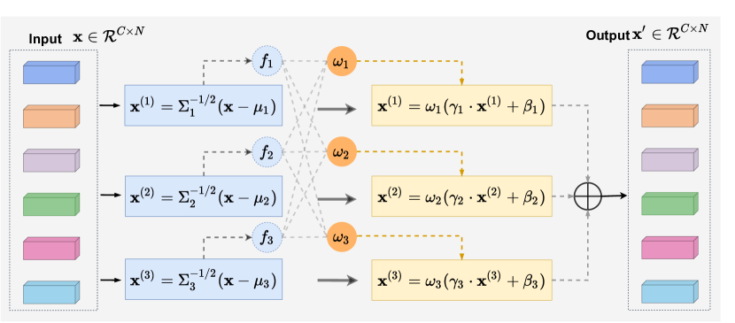
Figure 2. Compound batch normalization based on a mixture of Gaussian distributions.

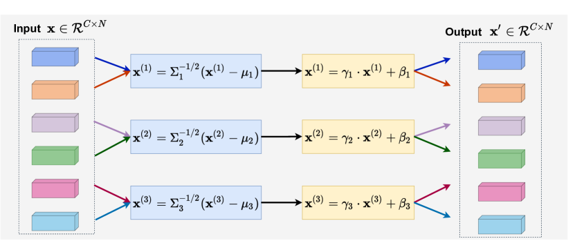
Figure 3. Split batch normalization.

Maximization Step. Temporary statistic parameters are estimated according to the probability values for each training batch. Practically, the temporary prior probability $\hat{\tau}_{j}^{c}$, mean $\hat{\bm{\mu}}_{j}^{c}$, and variance $\hat{\bm{\sigma}}_{j}^{c}$ of the $j$-th Gaussian distribution are calculated as below,

(10) $$\hat{\tau}_{j}^{c} =\frac{1}{N}\sum_{i=1}^{N}w_{ij},$$

(11) $$\hat{\bm{\mu}}_{j}^{c} =\frac{\sum_{i=1}^{N}w_{ij}\mathbf{x}_{i}}{\sum_{i=1}^{N}w_{ij}},$$

(12) $$\hat{\bm{\sigma}}_{j}^{c} =\frac{\sum_{i=1}^{N}w_{ij}(\mathbf{x}_{i}-\hat{\bm{\mu}}_{j})^{2}}{\sum_{i=1}^{N}w_{ij}}.$$

Temporal Accumulation. Similar to the conventional batch normalization, the moving average is applied to accumulate the above temporary variables, namely,

(13) $$\tau_{j} :=\lambda^{c}\tau_{j}+(1-\lambda^{c})\hat{\tau}_{j}^{c},$$

(14) $$\bm{\mu}_{j} :=\lambda^{c}\bm{\mu}_{j}+(1-\lambda^{c})\hat{\bm{\mu}}_{j}^{c},$$

(15) $$\bm{\Sigma}_{j} :=\lambda^{c}\bm{\Sigma}_{j}+(1-\lambda^{c})\textrm{diag}(\hat{\bm{\sigma}}_{j}).$$

Here, $\textrm{diag}(\cdot)$ transforms the input vector into a diagonal matrix, and $\lambda^{c}$ is a constant.

Finally, separate scaling and bias coefficients are learned to redistribute the values of different normalization branches. Those redistributed values are combined by the following weighted summation operation,

(16) $$\mathbf{x}^{\prime}_{i}=\sum_{j=1}^{M}w_{ij}(\gamma_{j}\hat{\textbf{x}}^{(j)}_{i}+\beta_{j}).$$

$\gamma_{j}$ and $\beta_{j}$ represent the scaling and bias coefficient of the $j$-th normalization branch respectively. The calculation process of the above normalization algorithm is illustrated in Figure 2. More details can be found in Appendix A.

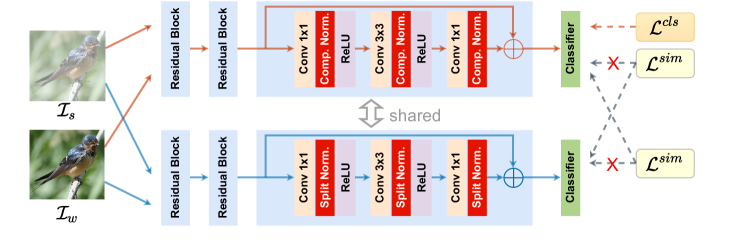
Figure 4. The proposed dual-path learning framework.

3.3. Split Batch Normalization

The generalized batch normalization can be easily incorporated into existing convolutional neural networks by replacing their original normalization layers. However, learning compound distributions with the expectation-maximization algorithm may easily fall into local optima and suffer from model collapse. To overcome this problem, we set up a split normalization strategy to diversify the Gaussian distributions with different sets of training samples.

First, we uniformly split all class labels into $M$ independent groups according to their serial numbers, resulting in $\{\mathbb{C}^{j}\}_{j=1}^{M}$, where $\mathbb{C}^{j}$ represents the $j$-th set of class labels. For $j\neq k$, $\mathbb{C}^{j}\cap\mathbb{C}^{k}=\varnothing$. The union of all class sets ($\cup_{j=1}^{M}\mathbb{C}^{j}$) is equal to the sequence of integers from 1 to the number of classes ($K$). According to these class sets, the input features in $\mathbf{x}$ can be separated into $M$ groups as well, namely $\{\mathbf{x}^{j}\in\mathbf{R}^{D\times N_{j}}\}_{j=1}^{M}$, where the features in $\mathbf{x}^{j}$ come from images with class labels in $\mathbb{C}^{j}$, and $N_{j}$ represents the number of features in the $j$-th group. Then, a split normalization strategy illustrated in Figure 3 is devised to process $M$ sets of features with $M$ Gaussian distributions, respectively. Meanwhile, each set of features is utilized for calculating the other temporary mean and variance,

(17) $$\hat{\bm{\mu}}_{j}^{s} =\frac{1}{n^{j}}\sum_{i=1}^{n^{j}}\mathbf{x}_{i}^{j},$$

(18) $$\hat{\bm{\sigma}}_{j}^{s} =\frac{1}{n^{j}}\sum_{i=1}^{n^{j}}(\mathbf{x}_{i}^{j}-\hat{\bm{\mu}}_{j}^{s})^{2}.$$

The above variables are also leveraged to update $\bm{\mu}_{j}$ and $\bm{\Sigma}_{j}$: $\bm{\mu}_{j}:=\lambda^{s}\bm{\mu}_{j}+(1-\lambda^{s})\hat{\bm{\mu}}_{j}^{s}$, and $\bm{\Sigma}_{j}:=\lambda^{s}\bm{\Sigma}_{j}+(1-\lambda^{s})\textrm{diag}(\hat{\bm{\sigma}}_{j}^{s})$. This process is beneficial for diversifying multiple Gaussian distributions and preventing the distribution collapse issue. The calculation process of the split batch normalization is illustrated in Algorithm 3 (Appendix A).

3.4. Dual-Path Learning

As shown in Figure 4, we build up the classification model with ResNet (He et al., 2016), which is learned with two branches. In the top branch, the compound normalization is applied for implementing the network feedforward process, while the split normalization is adopted for standardizing intermediate features in the bottom branch. Given an input image $\mathbf{I}\in\mathbb{R}^{3\times H\times W}$, we utilize a series of weak augmentation operations to transform it into $\mathbf{I}_{weak}$, and the other series of strong augmentation operations is leveraged to produce the other variant of the input image denoted by $\mathbf{I}_{strg}$. Feeding $\mathbf{I}_{weak}$ and $\mathbf{I}_{strg}$ into the branch based on the compound normalization, we can obtain predicted class-wise logits $\mathbf{o}^{c}_{weak}\in\mathbb{R}^{K\times 1}$ and $\mathbf{o}^{c}_{strg}\in\mathbb{R}^{K\times 1}$, respectively. $K$ denotes the number of classes. The split normalization branch also derives class-wise logits $\mathbf{o}^{s}_{weak}$ and $\mathbf{o}^{s}_{strg}$ from $\mathbf{I}_{weak}$ and $\mathbf{I}_{strg}$, respectively. The maximization of the similarity between predictions of two branches is employed for optimizing network parameters,

(19) $$L^{sim}=-\mathcal{S}(\mathbf{o}^{c}_{strg},\textrm{detach}(\mathbf{o}^{s}_{weak}))-\mathcal{S}(\mathbf{o}^{s}_{strg},\textrm{detach}(\mathbf{o}^{c}_{weak})).$$

Input: Training images: $\{\mathbf{I}_{l}\}_{l=1}^{L}$, and their labels: $\{\mathbf{y}_{l}\}_{l=1}^{L}$; $M$ sets of class labels: $\{\mathbb{C}^{j}\}_{j=1}^{M}$; $M$ sets of Gaussian statistic variables: $\{\tau_{j}\}_{j=1}^{M}$, $\{\bm{\mu}_{j}\}_{j=1}^{M}$, and $\{\bm{\Sigma}_{j}\}_{j=1}^{M}$.

Output: Optimized network parameters.

1:  Shuffle training images and separate into minibatches with size of $B$;

2:  for $i=1$ to $\frac{L}{B}$ do

3:     Fetch a batch of training images $\mathbf{B}\in\mathbb{R}^{B\times 3\times H\times W}$;

4:     Distort images in $\mathbf{B}$ with weak augmentation operations, resulting in $\mathbf{B}_{weak}$;

5:     Feed $\mathbf{B}_{weak}$ through the compound and split network paths, resulting in $\mathbf{O}^{c}_{weak}$ and $\mathbf{O}^{s}_{weak}$, respectively;

6:     Distort $\mathbf{B}$ with strong augmentation operations, deriving of $\mathbf{B}_{strg}$;

7:     Feed $\mathbf{B}_{strg}$ through the compound and split network paths, resulting in $\mathbf{O}^{c}_{strg}$ and $\mathbf{O}^{s}_{strg}$, respectively;

8:     Calculate training losses according to Eq. (19) and (20);

9:     Update network parameters by stochastic gradient descent;

10:  end for

Algorithm 1 Algorithm for one training epoch of the dual learning framework.

The similarity metric $\mathcal{S}(\mathbf{o}_{1},\mathbf{o}_{2})$ is implemented with the cosine function, $\mathcal{S}(\mathbf{o}_{1},\mathbf{o}_{2})=\mathbf{o}_{1}^{T}\mathbf{o}_{2}/(||\mathbf{o}_{1}||_{2}||\mathbf{o}_{2}||_{2})$. ‘$\textrm{detach}(\mathbf{o})$’ represents the stop gradient operation, which means $\mathbf{o}^{s}_{w}$ and $\mathbf{o}^{c}_{w}$ are regarded as constants.

Finally, the balanced softmax function is employed for calculating the training loss on the network prediction of strongly augmented image $\mathbf{I}_{strg}$,

(20) $$L^{cls}=-\log(\frac{n_{y}\exp(o^{c}_{strg}[y])}{\sum_{i=1}^{K}n_{i}\exp(o^{c}_{strg}[i])}).$$

$n_{i}$ denotes the number of samples in the $i$-th class, and $o^{c}_{strg}[i]$ is the $i$-th element in $\mathbf{o}^{c}_{strg}$. $y$ represents the ground-truth label of the input image $\mathbf{I}$. The practical training procedure is implemented with the minibatch size of $B$. One training epoch of the dual learning framework is summarized in Algorithm 1.

In training stage, the running variables(mean,variance and prior probability) of each Gaussian distribution are updated with temporal variables. During testing, the running variables are fixed, and only the calculation path of compound batch normalization is preserved while the path of split batch normalization is no longer used in the inference process of the model.

4. Experiments

We test the effectiveness of the proposed strategy on representative synthetic data as well as real-world datasets in this section. Table 1 describes the details of long-tailed data used in this work. The evaluation metric for image classification is top-1 accuracy (%).

4.1. Datasets

• CIFAR10-LT/100-LT. CIFAR10-LT/100-LT is formed by resampling images from the original CIFAR10-LT/100 (Krizhevsky et al., 2009) dataset. The class-wise sample sizes obey an exponential distribution. We denote the imbalance ratio as $\rho=N_{max}/N_{min}$, where $N_{max}$ and $N_{min}$ is the sample size of the most frequent class and the least frequent class, respectively. We validate the performance of all models under three settings for $\rho$ ($\in\{100,50,10\}$).

• ImageNet-LT. ImageNet-LT is a subset of the ImageNet1K (Russakovsky et al., 2015) dataset that contains images from 1000 categories, with a maximum of 1280 images per class and a minimum of 5 images per class. The dataset consists of 115.8k training images, 20k validation images, and 50k test images.

• Places-LT. Places-LT features an unbalanced training set from Places-2 (Zhou et al., 2017), with 62,500 images for 365 classes. The class frequencies are distributed according to a natural power law with a maximum of 4,980 images per class and a minimum of 5. The validation and testing sets are evenly distributed, with 20 and 100 images per class in each.

• iNaturalist2018 There are 437K images in iNaturalist-2018 (Van Horn et al., 2018), with 6 degrees of label granularity. This dataset is challenging since the labels are long-tailed and fine-grained. We only evaluate the most granular descriptors (species), resulting in 8142 distinct classes with a naturally imbalanced distribution.

  Table 1. Introduction of long-tailed datasets used in the experiments. Noted that $*$ means original data size in CIFAR10 and CIFAR100

  Dataset	Classs	$\rho$	Train	Val.	Test
  CIFAR10-LT	10	10-100	50k∗	-	10k
  CIFAR100-LT	100	10-100	50k∗	-	10k
  ImageNet-LT	1000	256	$\sim$115.8k	20k	50k
  Places-LT	365	996	62.5k	7.3k	36.5k
  iNaturalist2018	8142	500	$\sim$437.5k	$\sim$24.4k	$\sim$149.4k

4.2. Implementation Detail

Our method is implemented with PyTorch (Paszke et al., 2019). The weak augmentation is composed of random cropping and flipping, whereas AutoAugment (Cubuk et al., 2019) is used to generate strongly augmented images. We use SGD as the optimizer, with a learning rate of 0.05 that decays concerning the cosine annealing schedule. The number of training epochs is set to 400, and the mini-batch size is set to 128. $\lambda$, $\lambda^{c}$ and $\lambda^{s}$ are all set to 0.1. Without specification, the backbone is ResNet32, and all models are trained from scratch by default.

4.3. Ablation Studies

This section examines the efficacy of each component of the proposed approach and provides a detailed experimental study.

Table 2. Analysis of different components. The experiments are conducted on CIFAR10-LT and CIFAR100-LT, and we train the model from scratch for all cases. The ‘Baseline’ models are trained with AutoAugment (Cubuk et al., 2019) transforms and balanced loss (Ren et al., 2020). ‘SBN’ and ‘CBN’ indicate split batch normalization and compound batch normalization respectively. ‘DPL’ means dual path learning mentioned in Section 3.4. The number of mixtures M is empirically set to 4 for CBN.

Method	CIFAR10-LT			CIFAR100-LT
	$\rho$=100	$\rho$=50	$\rho$=10	$\rho$=100	$\rho$=50	$\rho$=10
Baseline	81.87	84.65	88.34	49.66	52.18	62.49
Baseline + SBN	82.03(+0.16)	84.73(+0.08)	88.89(+0.55)	49.86(+0.20)	52.44(+0.26)	62.55(+0.06)
Baseline + CBN	84.12(+2.25)	86.75(+2.10)	89.89(+1.55)	52.16(+2.50)	57.26(+5.08)	64.37(+1.88)
Baseline + CBN + SBN	84.31(+2.44)	87.21(+2.56)	90.44(+2.10)	52.76(+3.10)	58.04(+5.86)	64.97(+2.48)
Baseline + CBN + SBN + DPL	84.98(+3.11)	88.70(+4.05)	91.82(+3.48)	53.31(+3.65)	58.13(+5.95)	65.35(+2.86)

Components Analysis We conduct comprehensive ablation research to validate the essential components of our framework. Table 2 shows the results of the experiments. The loss criteria for evaluating the consistency between predictions and provided labels is the Balanced Softmax Cross-Entropy (Ren et al., 2020). As can be seen in Table 2, using CBN (compound batch normalization) improves performance significantly. For example, on the CIFAR10-LT dataset with $\rho=100$, the CBN results in a 2.25% increase in accuracy. The SBN (split batch normalization) assists in diversifying the statistical variables of multiple Gaussian distributions. The DPL (dual-path learning) approach, which was devised for feature learning, results in considerable performance gains. When $\rho$ is set to 100, 50, and 10, the accuracy of CIFAR100-LT is raised by 0.67%, 1.49%, and 1.38%, respectively.

Single-Modal Gaussian vs. Multi-Modal Gaussian. We first highlight the significance of compound normalization mentioned in section 3.2. We follow (Ren et al., 2020) to evaluate the classification accuracy on three disjoint sets of classes: many-shot (classes with more than 100 training samples), medium-shot (classes with 20–100 training samples), and few-shot (classes with fewer than 20 training samples). Figure 5 shows the top-1 accuracy against the number of mixtures on CIFAR100-LT. Here, balanced loss and dual-path learning are employed in this comparison. The plot demonstrates that estimating multiple Gaussian distributions favors all three subgroups. As can be seen that, multiple Gaussians (M¿1) are superior to single Gaussian (M=1) while too large M (larger than 4) cannot bring continuous performance gain since the difficulty of parameter estimation increases as M grows up. Apart from this, our proposed method causes subtle increase of computational burden compared to the baseline method. For example, when ResNet32 is used as the backbone, our model (M=4) occupies the space of 0.464M compared to original 0.461M in memory. Besides, the training process of the baseline and our approach consumes  3 hours and  4 hours respectively on CAFIR10-LT under imbalance factor of 100. The inference time difference between our method and the baseline can be very small.

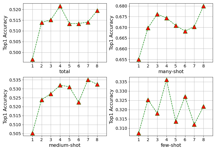
Figure 5. Performance of models trained with various numbers of Gaussian distributions on three disjoint subgroups. CIFAR100-LT with $\rho=100$ is used for training and testing.

Different Backbones. To test whether our method can generalize to other network architectures, we try to apply it to various variants of ResNet. The experimental results are presented in Figure 6. Unlike conventional residual networks, ResNet-20/32/44/56/110 is built upon three hyper-blocks. As can be observed, the proposed compound batch normalization consistently outperforms the conventional batch normalization across network architectures.

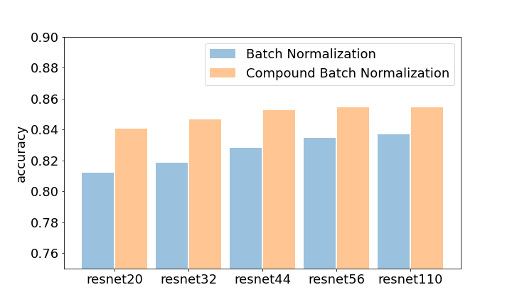
Figure 6. We test our technique on CIFAR10-LT with an imbalance factor of 100 and the number of mixtures is set to 4.

Combination with Re-sampling and Re-weighting We study the impact of CBN on data re-sampling/re-weighting algorithms in this subsection, by training our devised model with those algorithms. We accomplish decoupling training by decoupling the learning procedure into representation learning (80% epochs) and classification learning (20% epochs). The re-sampling/re-weighting method is only applied for fine-tuning parameters of classifiers during the classification learning stage while the parameters of the feature extractor are fixed. The backbone used in Table 3 is ResNet32, and we evaluate the top-1 accuracy on three disjoint subgroups on CIFAR100 with an imbalance factor of 100. We set (I) as the baseline that the model is trained with AutoAugment (Cubuk et al., 2019) transforms and balanced loss (Ren et al., 2020). Experiment (II) demonstrates that merely using re-sampling and decoupling training is ineffective in improving the accuracy. On the other hand, experiments (III) and (V) boost the baseline performance by promoting the accuracy on tail classes, but degrade the peformance on head classes. For our compound normalization, it delivers significant increases for most classes (except for ’Many’ in (VIII) and ’Few’ in (VI)) when combining re-weighting or re-sampling with decoupling training.

Table 3. Performance of our compound batch normalization (CBN) incorporated with data re-sampling (RS), data re-weighting (RW), and decoupling training (DT).

EXP	CBN	DT	RW	RS	Total	Many	Medium	Few
(I)	✗	✗	✗	✗	49.66	66.93	51.20	28.24
(II)	✗	✔	✗	✔	49.62	67.17	50.61	28.54
(III)	✗	✔	✔	✗	50.56	62.49	52.08	35.21
(IV)	✗	✔	✔	✔	50.66	60.73	52.47	37.07
(V)	✔	✗	✗	✗	52.16	69.26	54.18	30.34
(VI)	✔	✔	✗	✔	52.76	70.32	55.17	29.97
(VII)	✔	✔	✔	✗	52.83	69.34	55.58	30.82
(VIII)	✔	✔	✔	✔	52.86	68.65	55.61	31.67

4.4. Comparison with State-of-the-art Methods

We compare our method against existing algorithms, including MiSLAS (Zhong et al., 2021), LADE (Hong et al., 2021), ACE (Cai et al., 2021), DRO-LT (Samuel and Chechik, 2021), PaCo (Cui et al., 2021), DiVE (He et al., 2021), IB+Focal (Park et al., 2021), VS (Kini et al., 2021), TCM (Xu et al., 2021), DisAlign (Zhang et al., 2021d), and GistNet (Liu et al., 2021) on datasets mentioned in Table 1.

Results on CIFAR10-LT/100-LT. Table 4 summarizes the details, showing that all existing cutting-edge long-tailed approaches produce promising results. In comparison to previous approaches, our compound batch normalization properly accommodates the distribution shift between training and testing, resulting in a significant improvement. In particular, we attain an average precision of 85.0%/53.3%, whereas the available best of the rest is 82.8%/52.0% under imbalance condition $\rho=100$ for CIFAR10-LT and CIFAR100-LT, respectively. The compound normalization method can be considered of as a novel genre which is orthogonal to existing re-sampling, re-weighting strategies. More analysis can be noticed in Table 3.

Table 4. Comparison against other methods on CIFAR10-LT and CIFAR100-LT. ResNet32 is used as the backbone model.

Methods	CIFAR10-LT			CIFAR100-LT
	$\rho=100$	$\rho=50$	$\rho=10$	$\rho=100$	$\rho=50$	$\rho=10$
MiSLAS (Zhong et al., 2021)	82.1	85.7	90.0	47.0	52.3	63.2
LADE (Hong et al., 2021)	-	-	-	45.4	50.5	61.7
ACE (Cai et al., 2021)	81.4	84.9	-	49.6	51.9	-
DRO-LT (Samuel and Chechik, 2021)	-	-	-	47.3	57.6	63.4
PaCo (Cui et al., 2021)	-	-	-	52.0	56.0	64.2
DiVE (He et al., 2021)	-	-	-	45.4	51.1	62.0
SSD (Li et al., 2021b)	-	-	-	46.0	50.5	62.3
IB+Focal (Park et al., 2021)	78.0	82.4	87.9	45.0	48.9	59.5
VS (Kini et al., 2021)	80.8	-	-	43.5	-	-
TCM (Xu et al., 2021)	82.8	84.3	89.7	45.5	51.1	61.3
Ours	85.0	88.7	91.8	53.3	60.0	65.4

Results on ImageNet-LT. On ImageNet-LT, Table 5 presents detailed experimental results for comparisons with contemporary state-of-the-art algorithms using the ResNet50. We observe that PaCo (Cui et al., 2021) achieves comparable results (57.0%) that are slightly inferior to ours (57.4%). However, PaCo extends the contrastive framework MoCo (He et al., 2020; Chen et al., 2020) by introducing a new momentum encoder, which is much more demanding than our approach, to alleviate the long-tail problem. In addition to PaCo, our approach outperforms the remaining methods with an remarkable margin.

Table 5. Comparison against other methods on ImageNet-LT. ResNet50 is used as the backbone model.

Methods	Top-1 Accuracy
MiSLAS (Zhong et al., 2021)	52.7
DisAlign (Zhang et al., 2021d)	52.9
LADE (Hong et al., 2021)	52.0
ACE (Cai et al., 2021)	54.7
DRO-LT (Samuel and Chechik, 2021)	53.5
PaCo (Cui et al., 2021)	57.0
TCM (Xu et al., 2021)	48.4
Ours	57.4

Results on Places-LT. Places-LT is a long-tail variation of Places2 (Zhong et al., 2021). The studies are carried out using the backbone ResNet152 which is initialized with network parameters pre-trained on ImageNet. Table 6 demonstrates that our method consistently surpasses the state-of-the-art results with notable gains.

Table 6. Comparison against other methods on Places-LT. ResNet152 is used as the backbone model.

Methods	Top-1 Accuracy
MiSLAS (Zhong et al., 2021)	40.4
DisAlign (Zhang et al., 2021d)	39.3
LADE (Hong et al., 2021)	38.8
PaCo (Cui et al., 2021)	41.2
GistNet (Liu et al., 2021)	39.6
Ours	42.7

Results on iNaturalist2018. We examine our approach on the real-world long-tailed dataset iNaturalist 2018. Table 7 shows the experimental results. Our method outperforms contemporary state-of-the-art approaches such as PaCo (Cui et al., 2021), and ACE (Cai et al., 2021). The results indicate that our approach can handle extremely unbalanced fine-grained data in real-world scenarios despite the enormous number of classes.

Table 7. Comparison against other methods on iNaturalist 2018. ResNet50 is used as the backbone model.

Methods	Top-1 Accuracy
MiSLAS (Zhong et al., 2021)	71.6
DisAlign (Zhang et al., 2021d)	70.6
LADE (Hong et al., 2021)	70.0
ACE (Cai et al., 2021)	72.9
DRO-LT (Samuel and Chechik, 2021)	69.7
PaCo (Cui et al., 2021)	73.2
DiVE (He et al., 2021)	71.7
SSD (Li et al., 2021b)	71.5
IB+Focal (Park et al., 2021)	65.4
GistNet (Liu et al., 2021)	70.8
TCM (Xu et al., 2021)	69.2
Ours	74.8

5. Conclusion

This paper presents a compound batch normalization approach based on a mixture of Gaussian distributions that can comprehensively describe the feature space while avoiding the dominance of head classes. A moving average based expectation maximization (EM) method is introduced to capture the statistical variables for compound Gaussian distributions. The EM algorithm is sensitive to initialization and may easily get trapped in local minima. To tackle these issues, we build a dual-path learning approach that incorporates split feature normalization to diversify the Gaussian distributions. Extensive results on frequently used datasets show that the proposed method surpasses existing methods in long-tailed image classification by a considerable margin. To conclude, we present a novel perspective to address the imbalance issue at the feature level, which is inspiring to future work on this topic.

Appendix A Appendix

Input: Features: $\mathbf{x}\in\mathbb{R}^{D\times N}$; $M$ sets of Gaussian statistic variables: $\{\tau_{j}\}_{j=1}^{M}$, $\{\bm{\mu}_{j}\}_{j=1}^{M}$, and $\{\bm{\Sigma}_{j}\}_{j=1}^{M}$.

Output: Normalized features; updated Gaussian statistic variables.

1:  Standardize $\mathbf{x}$ with Gaussian distributions: $\hat{\textbf{x}}^{j}_{i}=\bm{\Sigma}^{-\frac{1}{2}}_{j}(\mathbf{x}_{i}-\bm{\mu}_{j})$, for $i\in[1,N]$ and $j\in[1,M]$;

2:  Calculate probabilities of input features in Gaussian distributions: $w_{ij}=\frac{\tau_{j}f(\mathbf{x}_{i},\bm{\mu}_{j},\bm{\Sigma}_{j})}{\sum_{k=1}^{M}\tau_{k}f(\mathbf{x}_{i},\mu_{k},\Sigma_{k})}$;

3:  Aggregate results of normalization branches: $\mathbf{x}^{\prime}_{i}=\sum_{j=1}^{M}w_{ij}(\gamma_{j}\hat{\textbf{x}}^{(j)}_{i}+\beta_{j})$;

4:  if training then

5:     Calculate temporary Gaussian statistic variables: $\hat{\tau}_{j}^{c}=\frac{1}{N}\sum_{i=1}^{N}w_{ij}$, $\hat{\bm{\mu}}_{j}^{c}=\frac{\sum_{i=1}^{N}w_{ij}\mathbf{x}_{i}}{\sum_{i=1}^{N}w_{ij}}$, and $\hat{\bm{\sigma}}_{j}^{c}=\frac{\sum_{i=1}^{N}w_{ij}(\mathbf{x}_{i}-\hat{\bm{\mu}}_{j}^{c})^{2}}{\sum_{i=1}^{N}w_{ij}}$;

6:     Update permanent Gaussian statistic variables: $\tau_{j}\leftarrow\lambda^{c}\tau_{j}+(1-\lambda^{c})\hat{\tau}_{j}^{c}$, $\bm{\mu}_{j}\leftarrow\lambda^{c}\bm{\mu}_{j}+(1-\lambda^{c})\hat{\bm{\mu}}_{j}^{c}$, and $\bm{\Sigma}_{j}\leftarrow\lambda^{c}\bm{\Sigma}_{j}+(1-\lambda^{c})\textrm{diag}(\hat{\bm{\sigma}}_{j}^{c})$.

7:  end if

Algorithm 2 Algorithm for the calculation process of the generalized batch normalization.

Input: Features: $\mathbf{x}\in\mathbb{R}^{D\times N}$, and their labels: $\mathbf{y}\in\mathbb{R}^{N}$; $M$ sets of class labels: $\{\mathbb{C}^{j}\}_{j=1}^{M}$; $M$ sets of Gaussian statistic variables: $\{\tau_{j}\}_{j=1}^{M}$, $\{\bm{\mu}_{j}\}_{j=1}^{M}$, and $\{\bm{\Sigma}_{j}\}_{j=1}^{M}$.

Output: Normalized features; updated Gaussian statistic variables.

1:  Initialize feature groups: $\mathbf{x}^{j}=[]$, for $j\in[1,M]$;

2:  for $i=1$ to $N$ do

3:     Retrieve the index of label class set $s_{i}$ which $\mathbf{x}_{i}$’s label belongs to;

4:     Append $\mathbf{x}_{i}$ into $\mathbf{x}^{s_{i}}$;

5:  end for

6:  for $j=1$ to $M$ do

7:     Normalize $\mathbf{x}^{j}$ with the $j$-th Gaussian distribution: $\hat{\textbf{x}}^{j}=\bm{\Sigma}^{-\frac{1}{2}}_{j}(\mathbf{x}^{j}-\bm{\mu}_{j})$;

8:     Redistribute $\hat{\mathbf{x}}^{j}$ with the affine parameters of the $j$-th normalization branch: $\mathbf{x}^{j\prime}=\gamma_{j}\hat{\textbf{x}}^{j}+\beta_{j}$;

9:     if training then

10:        Calculate temporary Gaussian statistic variables: $\hat{\bm{\mu}}_{j}^{s}=\sum_{i=1}^{N_{j}}\mathbf{x}_{i}^{j}/N_{j}$, and $\hat{\bm{\sigma}}_{j}^{s}=\sum_{i=1}^{N_{j}}(\mathbf{x}_{i}^{j}-\hat{\bm{\mu}}_{j}^{s})^{2}/N_{j}$, where $N_{j}$ denotes the number of features in $\mathbf{x}^{j}$;

11:        Update permanent Gaussian statistic variables: $\bm{\mu}_{j}\leftarrow\lambda^{s}\bm{\mu}_{j}+(1-\lambda^{s})\hat{\bm{\mu}}_{j}^{s}$, and $\bm{\Sigma}_{j}\leftarrow\lambda^{s}\bm{\Sigma}_{j}+(1-\lambda^{s})\textrm{diag}(\hat{\bm{\sigma}}_{j}^{s})$.

12:     end if

13:  end for

Algorithm 3 Algorithm for the calculation process of the split batch normalization.

References

- (1)
- Ba et al. (2016) Jimmy Lei Ba, Jamie Ryan Kiros, and Geoffrey E Hinton. 2016. Layer normalization. arXiv preprint arXiv:1607.06450 (2016).
- Cai et al. (2021) Jiarui Cai, Yizhou Wang, and Jenq-Neng Hwang. 2021. Ace: Ally complementary experts for solving long-tailed recognition in one-shot. In Proceedings of the IEEE/CVF International Conference on Computer Vision. 112–121.
- Cao et al. (2019) Kaidi Cao, Colin Wei, Adrien Gaidon, Nikos Arechiga, and Tengyu Ma. 2019. Learning imbalanced datasets with label-distribution-aware margin loss. Advances in neural information processing systems 32 (2019).
- Chawla et al. (2002) Nitesh V Chawla, Kevin W Bowyer, Lawrence O Hall, and W Philip Kegelmeyer. 2002. SMOTE: synthetic minority over-sampling technique. Journal of artificial intelligence research 16 (2002), 321–357.
- Chen et al. (2021) Junya Chen, Zidi Xiu, Benjamin Goldstein, Ricardo Henao, Lawrence Carin, and Chenyang Tao. 2021. Supercharging Imbalanced Data Learning With Energy-based Contrastive Representation Transfer. Advances in Neural Information Processing Systems 34 (2021).
- Chen et al. (2020) Xinlei Chen, Haoqi Fan, Ross Girshick, and Kaiming He. 2020. Improved baselines with momentum contrastive learning. arXiv preprint arXiv:2003.04297 (2020).
- Chen and He (2021) Xinlei Chen and Kaiming He. 2021. Exploring simple siamese representation learning. In Proceedings of the IEEE/CVF Conference on Computer Vision and Pattern Recognition. 15750–15758.
- Cheng et al. (2021) Lechao Cheng, Zunlei Feng, Xinchao Wang, Ya Jie Liu, Jie Lei, and Mingli Song. 2021. Boundary Knowledge Translation based Reference Semantic Segmentation. arXiv preprint arXiv:2108.01075 (2021).
- Cheng et al. (2018) Lechao Cheng, Chengyi Zhang, and Zicheng Liao. 2018. Intrinsic image transformation via scale space decomposition. In Proceedings of the IEEE conference on computer vision and pattern recognition. 656–665.
- Chu et al. (2020) Peng Chu, Xiao Bian, Shaopeng Liu, and Haibin Ling. 2020. Feature space augmentation for long-tailed data. In European Conference on Computer Vision. Springer, 694–710.
- Cubuk et al. (2019) Ekin D Cubuk, Barret Zoph, Dandelion Mane, Vijay Vasudevan, and Quoc V Le. 2019. Autoaugment: Learning augmentation strategies from data. In Proceedings of the IEEE/CVF Conference on Computer Vision and Pattern Recognition. 113–123.
- Cui et al. (2021) Jiequan Cui, Zhisheng Zhong, Shu Liu, Bei Yu, and Jiaya Jia. 2021. Parametric contrastive learning. In Proceedings of the IEEE/CVF International Conference on Computer Vision. 715–724.
- Cui et al. (2019) Yin Cui, Menglin Jia, Tsung-Yi Lin, Yang Song, and Serge Belongie. 2019. Class-balanced loss based on effective number of samples. In Proceedings of the IEEE/CVF conference on computer vision and pattern recognition. 9268–9277.
- Drummond et al. (2003) Chris Drummond, Robert C Holte, et al. 2003. C4. 5, class imbalance, and cost sensitivity: why under-sampling beats over-sampling. In Workshop on learning from imbalanced datasets II, Vol. 11. Citeseer, 1–8.
- Hao et al. (2022) Yanbin Hao, Hao Zhang, Chong-Wah Ngo, and Xiangnan He. 2022. Group Contextualization for Video Recognition. In Proceedings of the IEEE/CVF Conference on Computer Vision and Pattern Recognition. 928–938.
- He et al. (2020) Kaiming He, Haoqi Fan, Yuxin Wu, Saining Xie, and Ross Girshick. 2020. Momentum contrast for unsupervised visual representation learning. In Proceedings of the IEEE/CVF conference on computer vision and pattern recognition. 9729–9738.
- He et al. (2016) Kaiming He, Xiangyu Zhang, Shaoqing Ren, and Jian Sun. 2016. Deep residual learning for image recognition. In Proceedings of the IEEE conference on computer vision and pattern recognition. 770–778.
- He et al. (2021) Yin-Yin He, Jianxin Wu, and Xiu-Shen Wei. 2021. Distilling virtual examples for long-tailed recognition. In Proceedings of the IEEE/CVF International Conference on Computer Vision. 235–244.
- Hong et al. (2021) Youngkyu Hong, Seungju Han, Kwanghee Choi, Seokjun Seo, Beomsu Kim, and Buru Chang. 2021. Disentangling label distribution for long-tailed visual recognition. In Proceedings of the IEEE/CVF Conference on Computer Vision and Pattern Recognition. 6626–6636.
- Huang et al. (2016) Chen Huang, Yining Li, Chen Change Loy, and Xiaoou Tang. 2016. Learning deep representation for imbalanced classification. In Proceedings of the IEEE conference on computer vision and pattern recognition. 5375–5384.
- Ioffe and Szegedy (2015) Sergey Ioffe and Christian Szegedy. 2015. Batch normalization: Accelerating deep network training by reducing internal covariate shift. In International conference on machine learning. PMLR, 448–456.
- Kini et al. (2021) Ganesh Ramachandra Kini, Orestis Paraskevas, Samet Oymak, and Christos Thrampoulidis. 2021. Label-imbalanced and group-sensitive classification under overparameterization. Advances in Neural Information Processing Systems 34 (2021).
- Krizhevsky et al. (2009) Alex Krizhevsky, Geoffrey Hinton, et al. 2009. Learning multiple layers of features from tiny images. (2009).
- Li et al. (2021a) Shuang Li, Kaixiong Gong, Chi Harold Liu, Yulin Wang, Feng Qiao, and Xinjing Cheng. 2021a. Metasaug: Meta semantic augmentation for long-tailed visual recognition. In Proceedings of the IEEE/CVF Conference on Computer Vision and Pattern Recognition. 5212–5221.
- Li et al. (2021b) Tianhao Li, Limin Wang, and Gangshan Wu. 2021b. Self supervision to distillation for long-tailed visual recognition. In Proceedings of the IEEE/CVF International Conference on Computer Vision. 630–639.
- Lin et al. (2017) Tsung-Yi Lin, Priya Goyal, Ross Girshick, Kaiming He, and Piotr Dollár. 2017. Focal loss for dense object detection. In Proceedings of the IEEE international conference on computer vision. 2980–2988.
- Liu et al. (2021) Bo Liu, Haoxiang Li, Hao Kang, Gang Hua, and Nuno Vasconcelos. 2021. GistNet: a Geometric Structure Transfer Network for Long-Tailed Recognition. In Proceedings of the IEEE/CVF International Conference on Computer Vision. 8209–8218.
- Liu et al. (2020) Jialun Liu, Yifan Sun, Chuchu Han, Zhaopeng Dou, and Wenhui Li. 2020. Deep representation learning on long-tailed data: A learnable embedding augmentation perspective. In Proceedings of the IEEE/CVF Conference on Computer Vision and Pattern Recognition. 2970–2979.
- Merchant et al. (2020) Amil Merchant, Barret Zoph, and Ekin Dogus Cubuk. 2020. Does data augmentation benefit from split batchnorms. arXiv preprint arXiv:2010.07810 (2020).
- Park et al. (2021) Seulki Park, Jongin Lim, Younghan Jeon, and Jin Young Choi. 2021. Influence-balanced loss for imbalanced visual classification. In Proceedings of the IEEE/CVF International Conference on Computer Vision. 735–744.
- Paszke et al. (2019) Adam Paszke, Sam Gross, Francisco Massa, Adam Lerer, James Bradbury, Gregory Chanan, Trevor Killeen, Zeming Lin, Natalia Gimelshein, Luca Antiga, et al. 2019. Pytorch: An imperative style, high-performance deep learning library. Advances in neural information processing systems 32 (2019).
- Ren et al. (2020) Jiawei Ren, Cunjun Yu, Shunan Sheng, Xiao Ma, Haiyu Zhao, Shuai Yi, and Hongsheng Li. 2020. Balanced Meta-Softmax for Long-Tailed Visual Recognition. In Proceedings of Neural Information Processing Systems(NeurIPS).
- Russakovsky et al. (2015) Olga Russakovsky, Jia Deng, Hao Su, Jonathan Krause, Sanjeev Satheesh, Sean Ma, Zhiheng Huang, Andrej Karpathy, Aditya Khosla, Michael Bernstein, et al. 2015. Imagenet large scale visual recognition challenge. International journal of computer vision 115, 3 (2015), 211–252.
- Samuel and Chechik (2021) Dvir Samuel and Gal Chechik. 2021. Distributional robustness loss for long-tail learning. In Proceedings of the IEEE/CVF International Conference on Computer Vision. 9495–9504.
- Van Horn et al. (2018) Grant Van Horn, Oisin Mac Aodha, Yang Song, Yin Cui, Chen Sun, Alex Shepard, Hartwig Adam, Pietro Perona, and Serge Belongie. 2018. The inaturalist species classification and detection dataset. In Proceedings of the IEEE conference on computer vision and pattern recognition. 8769–8778.
- Wang et al. (2020) Xudong Wang, Long Lian, Zhongqi Miao, Ziwei Liu, and Stella X Yu. 2020. Long-tailed recognition by routing diverse distribution-aware experts. arXiv preprint arXiv:2010.01809 (2020).
- Wang et al. (2019) Yulin Wang, Xuran Pan, Shiji Song, Hong Zhang, Gao Huang, and Cheng Wu. 2019. Implicit semantic data augmentation for deep networks. Advances in Neural Information Processing Systems 32 (2019).
- Wang et al. (2017) Yu-Xiong Wang, Deva Ramanan, and Martial Hebert. 2017. Learning to model the tail. Advances in Neural Information Processing Systems 30 (2017).
- Wu and He (2018) Yuxin Wu and Kaiming He. 2018. Group normalization. In Proceedings of the European conference on computer vision (ECCV). 3–19.
- Xiang et al. (2020) Liuyu Xiang, Guiguang Ding, and Jungong Han. 2020. Learning from multiple experts: Self-paced knowledge distillation for long-tailed classification. In European Conference on Computer Vision. Springer, 247–263.
- Xu et al. (2021) Zhengzhuo Xu, Zenghao Chai, and Chun Yuan. 2021. Towards Calibrated Model for Long-Tailed Visual Recognition from Prior Perspective. Advances in Neural Information Processing Systems 34 (2021).
- Zada et al. (2021) Shiran Zada, Itay Benou, and Michal Irani. 2021. Pure Noise to the Rescue of Insufficient Data: Improving Imbalanced Classification by Training on Random Noise Images. arXiv preprint arXiv:2112.08810 (2021).
- Zhang et al. (2021a) Dingwen Zhang, Junwei Han, Gong Cheng, and Ming-Hsuan Yang. 2021a. Weakly supervised object localization and detection: A survey. IEEE transactions on pattern analysis and machine intelligence (2021).
- Zhang et al. (2020) Dingwen Zhang, Wenyuan Zeng, Jieru Yao, and Junwei Han. 2020. Weakly supervised object detection using proposal-and semantic-level relationships. IEEE Transactions on Pattern Analysis and Machine Intelligence (2020).
- Zhang et al. (2021b) Hao Zhang, Yanbin Hao, and Chong-Wah Ngo. 2021b. Token shift transformer for video classification. In Proceedings of the 29th ACM International Conference on Multimedia. 917–925.
- Zhang et al. (2021d) Songyang Zhang, Zeming Li, Shipeng Yan, Xuming He, and Jian Sun. 2021d. Distribution alignment: A unified framework for long-tail visual recognition. In Proceedings of the IEEE/CVF Conference on Computer Vision and Pattern Recognition. 2361–2370.
- Zhang et al. (2021c) Yifan Zhang, Bryan Hooi, Lanqing Hong, and Jiashi Feng. 2021c. Test-agnostic long-tailed recognition by test-time aggregating diverse experts with self-supervision. arXiv preprint arXiv:2107.09249 (2021).
- Zhong et al. (2021) Zhisheng Zhong, Jiequan Cui, Shu Liu, and Jiaya Jia. 2021. Improving calibration for long-tailed recognition. In Proceedings of the IEEE/CVF Conference on Computer Vision and Pattern Recognition. 16489–16498.
- Zhou et al. (2020) Boyan Zhou, Quan Cui, Xiu-Shen Wei, and Zhao-Min Chen. 2020. Bbn: Bilateral-branch network with cumulative learning for long-tailed visual recognition. In Proceedings of the IEEE/CVF conference on computer vision and pattern recognition. 9719–9728.
- Zhou et al. (2017) Bolei Zhou, Agata Lapedriza, Aditya Khosla, Aude Oliva, and Antonio Torralba. 2017. Places: A 10 million Image Database for Scene Recognition. IEEE Transactions on Pattern Analysis and Machine Intelligence (2017).