[1]
[type=editor, auid=000,bioid=1, orcid=0000-0001-8675-0184]
[1]
[1]This research did not receive any specific grant from funding agencies in the public, commercial, or not-for-profit sectors. \cortext[cor1]Corresponding author
In this work we proposed a new algorithm which can automatically find cluster in high-dimensional data feature space in a simple way.
Clustering through Feature Space Sequence Discovery and Analysis
Abstract
Identifying high-dimensional data patterns without a priori knowledge is an important task of data science. This paper proposes a simple and efficient noparametric algorithm: Data Convert to Sequence Analysis, DCSA, which dynamically explore each point in the feature space without repetition, and a Directed Hamilton Path will be found. Based on the change point analysis theory, The sequence corresponding to the path is cut into several fragments to achieve clustering. The experiments on real-world datasets from different fields with dimensions ranging from 4 to 20531 confirm that the method in this work is robust and has visual interpretability in result analysis.
keywords:
Clustering\sepHigh-dimensional\sepSequence analysis \sepHamiltonian Path1 Introduction
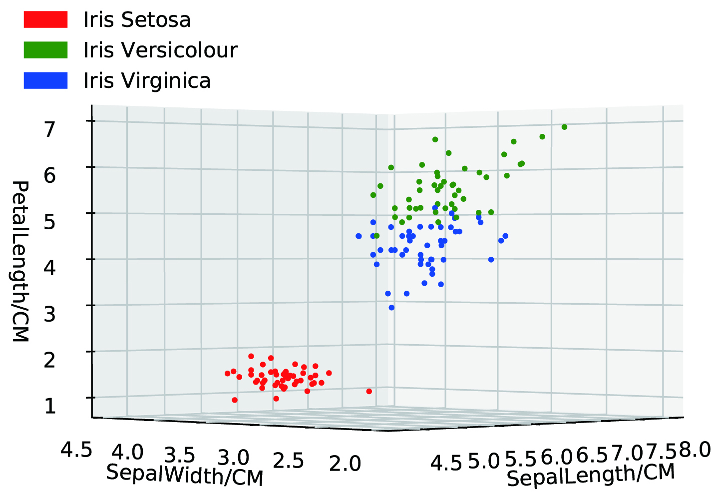
Data points are embedded in the feature space constructed by their attributes. If the data has a natural classification, its spatial structure may have several forms of distinguishability. Figure 1 is a 3D image generated by the Iris data set[1] with three attributes. It is noticed that the red class is obviously distinguished from other two classes. We assume that the information is compressed in all dimensions, if all four dimensions can be used and displayed, the distinguishability of the blue and green categories in Figure 1 will be more obvious.
In this work, we designed a Data Convert To Sequence Analysis Algorithm (DCSA) to prove this hypothesis. The DCSA is capable to explore the space constructed by full-dimensional of data, looking for the distinguishable clues, and then discover clusters. In this paper, the terminology “multi-dimension” refers to space dimension with more than 3, while “high-dimension” referes to space dimension frome dozens to ten thousands.
The DCSA takes the euclidean distance of data points to generate a directed Hamilton Path[2] to connect all points. The distance between every two points on the path forms a sequence which is further divided into fragments using sequence analysis technology, and each segment is considered as a class.
The traditional clustering method has successfully solved the clustering problem of low-dimensional data[3].However, the clustering of the multi-dimension, especially the high-dimensional data is more complicated because of the following reasons:
1. The probability of cluster structure in the full attributes feature space is lower;
2. The data distribution in the high-dimensional space is more sparse, which has an effect on the discovery of cluster structure.
High-dimensional data pattern recognition several methods proposed in the literature: such as dimensionality reduction[4], regularization-based technology[5], parsimonious modeling [6], subspace clustering[7] and variable selection-based clustering[8]. The dimensionality reduction method is classified as follows:
DCSA is a dimensionality reduction algorithm based on distance preserving global attributes.
2 Data Convert To Sequence
2.1 2.1 Sequence discovery
Feature space of the dataset exists directed graph[9] , which is a graph, where is the number of sample points, and is the edge that connect all points. If there exists a graph in which represents a path and each vertex for G was visited exactly once, and , then identifies a Hamiltonian path.
The DCSA algorithm for finding the Hamiltonian path is shown in the Algorithm1:
Its time complexity is . In fact, it is not necessary to calculate the Gram matrix, just randomly choose a starting point, and the rest is determined by dynamic planning. Otherwise, when the sample over 100,000, the size of G will exceed 70GB because of Gram matrix space complexity is . We calculate G to ensure that the experiment can be reproduced. If a starting point is randomly selected, the time complexity of the algorithm will be reduced to , and space complexity will sharply reduced to .
The method to find the starting point in Setp4 is as follows:
The row index of the distance matrix represents the ordinal number of the data element, and the row sums of represents the total distance from the element to the others, including itself. The row index which has the smallest row-sum can be regarded as the center of a highest density area.
The order of the value, is the right sequence we are looking for, here marked as .
The time complexity of Step 3-5 is , and the total time complexity of steps 0-6 is .
DCSA is a dynamic programming algorithm, and its model is as follows:
| (3) |
where represents the entire decision-making process from the starting point 1 to the end point . represents the set of decisions in the state .In this paper:
where ,
The process of the algorithm for finding the Hamiltonian path is a Markov decision process[12, 13, 14]. The current state is only affected by its previous state and has nothing to do with the other historical states. The formal expression is as follows:
| (4) |
Generally speaking, in the data convert to sequence stage, we assume that there is a discovery factor (DF), which will explore points in an dimensional space. The starting time for exploration is , and the starting point is obtained by calculation .DF starts from the current point to the next one with the closest Euclidean distance, and does not visit a point twice. After time, it will visit all points and arrive , leaving an exploration path composed of distances.
The experiment for DCSA shows that the majority of the same class point is concentrated in the same interval of the sequence.
The actual exploration process of DCSA on the original iris data set is shown in Figure 2A to C. The purple, cyan, and green represent iris-setosa, iris-versicolour, and iris-virginica, respectively.
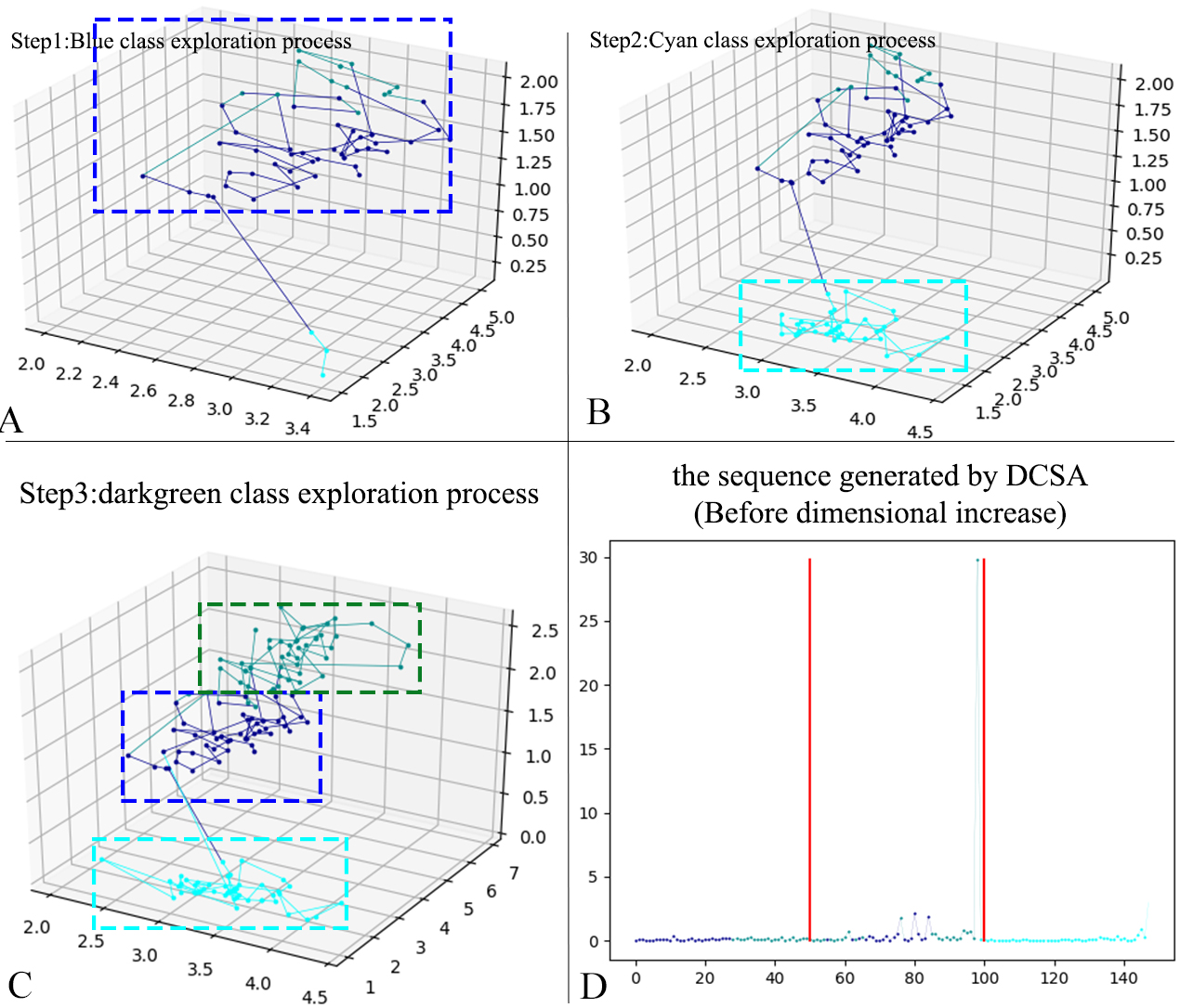
It is shown that the DCSA exploration is carried out in a priority class, especially the cyan with a large distance from other classes has 100% exploration continuity. The purple class and the green class are overlap in space, leading to alternate exploration processes. We speculate that the DCSA application will have better results by mapping data to higher dimensions through the kernel method[15].Figure 2D shows the coloring result of the DCSA generated sequence.
2.2 Data standardization
The DCSA is sensitive to the differences in the value range of data attributes, and such data needs to be standardized pre-processing[16].
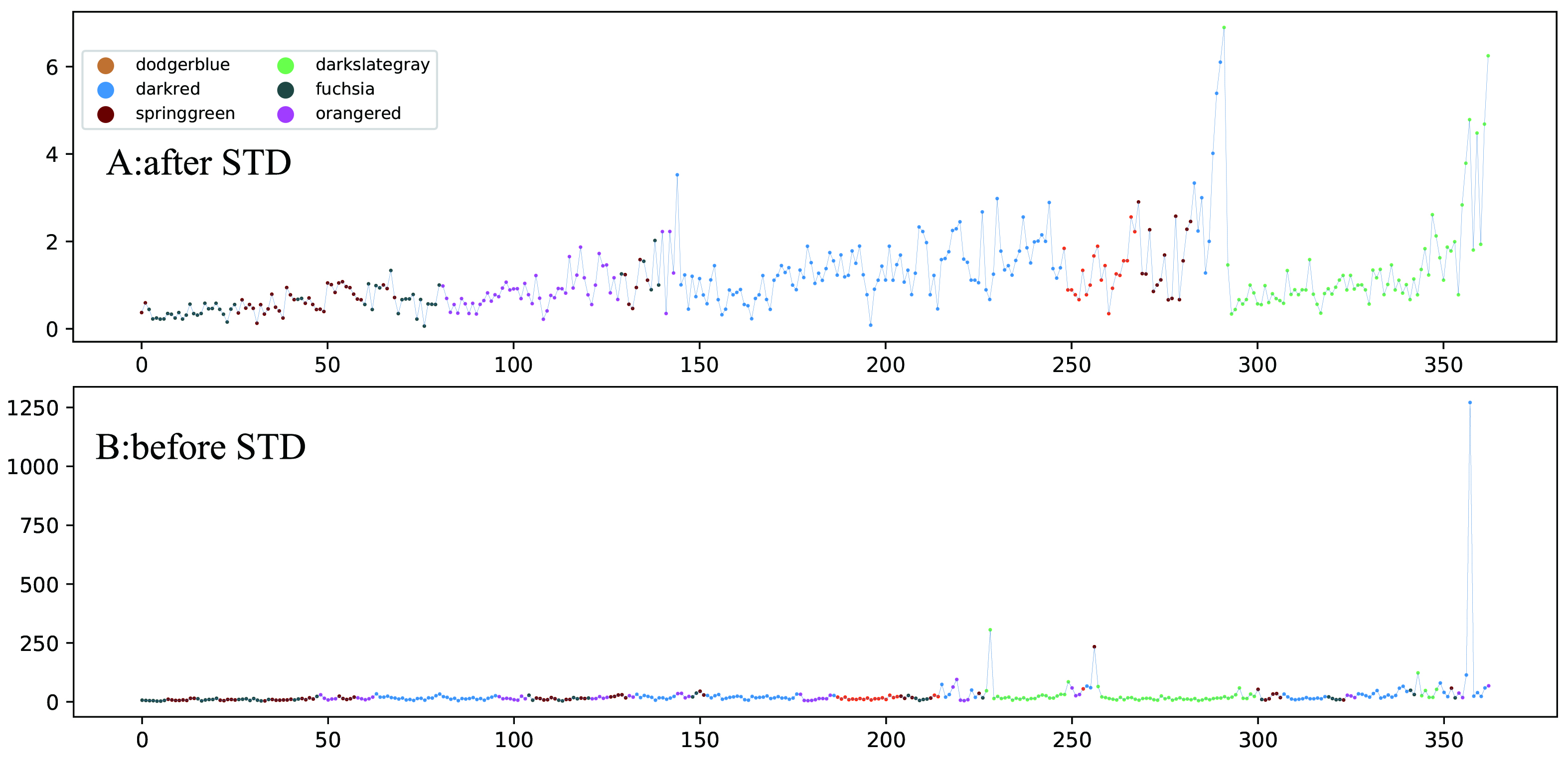
As shown in Figure3, the obviously enhancement for the regularity can be seen after standardization. With coloring the sequence by class, it is clearly showed that the effectiveness of the algorithm DCSA after standardization.
2.3 Low-dimensional data application DCSA
It is noticed in Figure 2D that the DCSA application is not ideal, resulting from that the Iris has only four attributes. Therefore, we use polynomial kernel[17] to increase the dimension for the further application of the DCSA. The result is plotted in Figure 4, of which the red vertical line is the known dividing point.
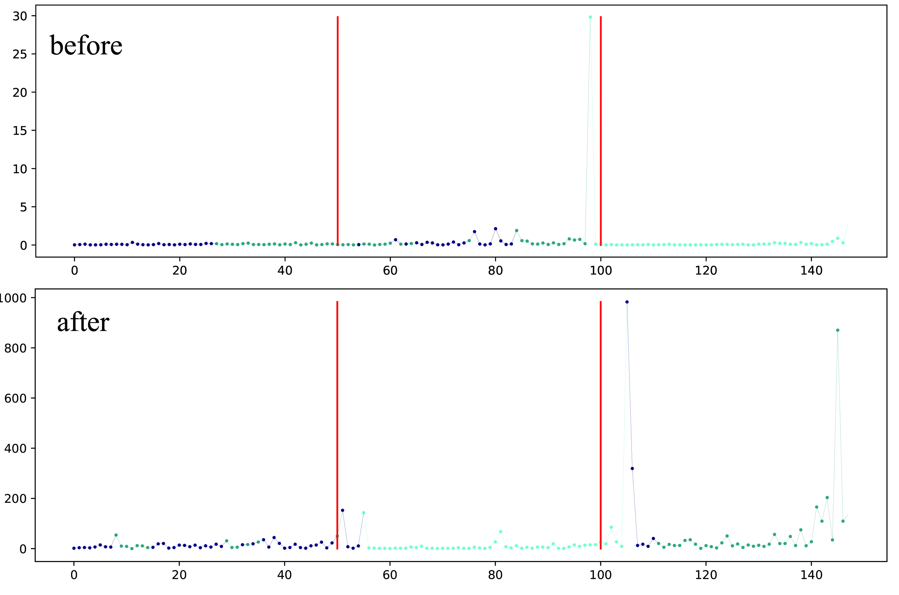
After increasing the dimension, the sequence has obvious jumps between different classes. It is demonstrated that the continuity of similar data points in the same interval is enhanced and the effect of the DCSA is also improved.
3 Sequence Analysis
3.1 Theoretical basis
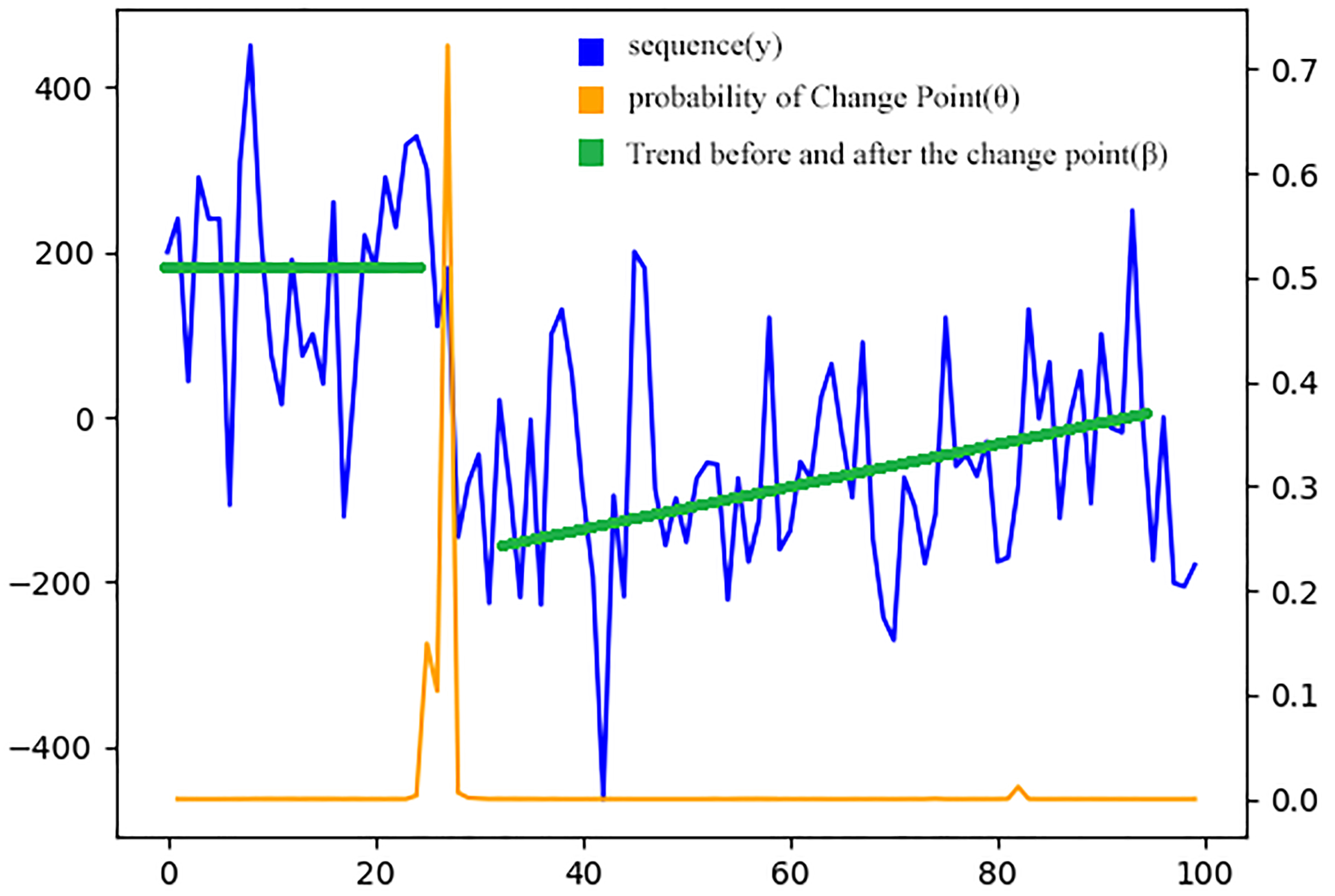
Li A. G. et al.[18] supported that sequence truncation, segmentation, clustering, etc. could be unified into Sequence Change Point Analysis (SCPA) problem, First we divide the sequence into 1-K segments, and each segment obeys one of the orthogonal transformation model set M (M can be linear polynomial model, wavelet transform Fourier transform model etc). The problem of sequence change point is shown in Figure 5, where the sequence before and after the change point is represented by a linear model (green line). This is also an optimal segmentation problem.
3.2 Mathematical modeling
The optimal segmentation problem is modeled as follows. The segment modeling for original sequence is as follows:
Where is the function representation of each segment, is noise, and is the segment point. The objective function is to minimize the mean-square error(MSE) distance between segment function and those points in this segment:
is the number of samples in segment . If the number of segments is not limited, and every two points can be identified as a segment, the objective function value is 0. Therefore the following constraints are required:
The above is the basic method for sequence change point discovery. The application based on the above theory are further detailed in the following section.
3.3 Related algorithms
In present papper, we select four sequence analysis algorithms: BCD,CUSUM,ARIMA,JNBD. The BCD algorithm is a newer algorithm, which will be detailedly described here, and only a brief introduction of other three methods will be given here, due to they are all well-known algorithms.
3.3.1 BCD algorithm
Xiang et al.[19, 20, 21, 22] used Bayesian method to calculate the probability of change points (Bayesian Changepoint Detection, BCD). Similar to the theoretical basis, the problem is transformed into a mixed linear model containing change points:
| (5) |
Where is the linear fitting coefficient before and after the discontinuity point, which is used to describe the changing trend of the sequence before and after the change point; is the noise, is the variance matrix; is the step function, which is used to distinguish between before and after the change point:
The above model(5) can be rewritten as:
| (6) |
Applying Bayesian formula, we have
| (7) |
when is known as an observation, and the equivalent equation as:
| (8) |
We take the hidden variable (change point) into consideration, and the corresponding likelihood equation of Formula (6) is:
| (9) |
This is the likelihood function form of Formula 6, which is corresponded to Bayesian function Formula 8.
Parameter is unknown, there must be a that maximizes the likelihood equation:
| (10) |
where , is the residual.
Assuming that all parameters are independent, then:
Integrate and to get . Those points which is corresponded to the largest is the division point of the sequence.
The experiment in this paper used the BCD implementation library from python: bayesian_changepoint_detection.
3.3.2 CUSUM algorithm
Cumulative Sum Control Chart[23, 24] (CUSUM) is a sequential analysis method that accumulates small deviations in the process to achieve the effect of amplification, leading to an improvement on the sensitivity to small deviations during the detection process. When CUSUM detects the cumulative deviation is significantly higher or lower than the average level under normal and stable operating conditions, it means that the system has changed. The self-edited algorithm CUSUM-A and the Python package detectaḋetect_cusum(CUSUM-B) are applied in this work.
3.3.3 ARIMA algorithm
Autoregressive Integrated Moving Average model[25](ARIMA) has three parameters (p, d, q), p is the number of autoregressive items; MA is "moving average", q is the number of moving average items, and d is the number of items that delive a stationary sequence. The ARIMA model can be expressed as:
is Lag operator, .
The experiment in this paper used the ARIMA implementation library from python: Change_Finder.
3.3.4 JNBD algorithm
Finally we applied the Jenks natural breaks points detection algorithm[26] (JNBD). This method is almost completely consistent with the method introduced in the theoretical basis. Initializing random breakpoints, and then iteratively calculating different breakpoint position, The truncation principle is to maximize variance between groups and minimize variance within groups. Corresponding library in Python is jenkspy.
4 Experiments
The experimental are performed in the following computational configuration: IntelXeonSilver4110 CPU 2.10GHz, 48GB DDR4 memory and Windows10-64bit enterprise operating system with Python 3.7.
4.1 Application of artificial data sets
4.1.1 Overall performance test
Figure 6 is shows an overall comparison between DCSA and some classic clustering algorithms on the low-dimensional generated dataset(a:’noisy_circles’, b:’noisy_moons’, c:’blobs’, d:’aniso’, e:’varied’).The AMI score is in the lower left corner of each chart, and the elapsed time is in the lower right foot. It is obvious that K-means algorithm has the best operating efficiency.
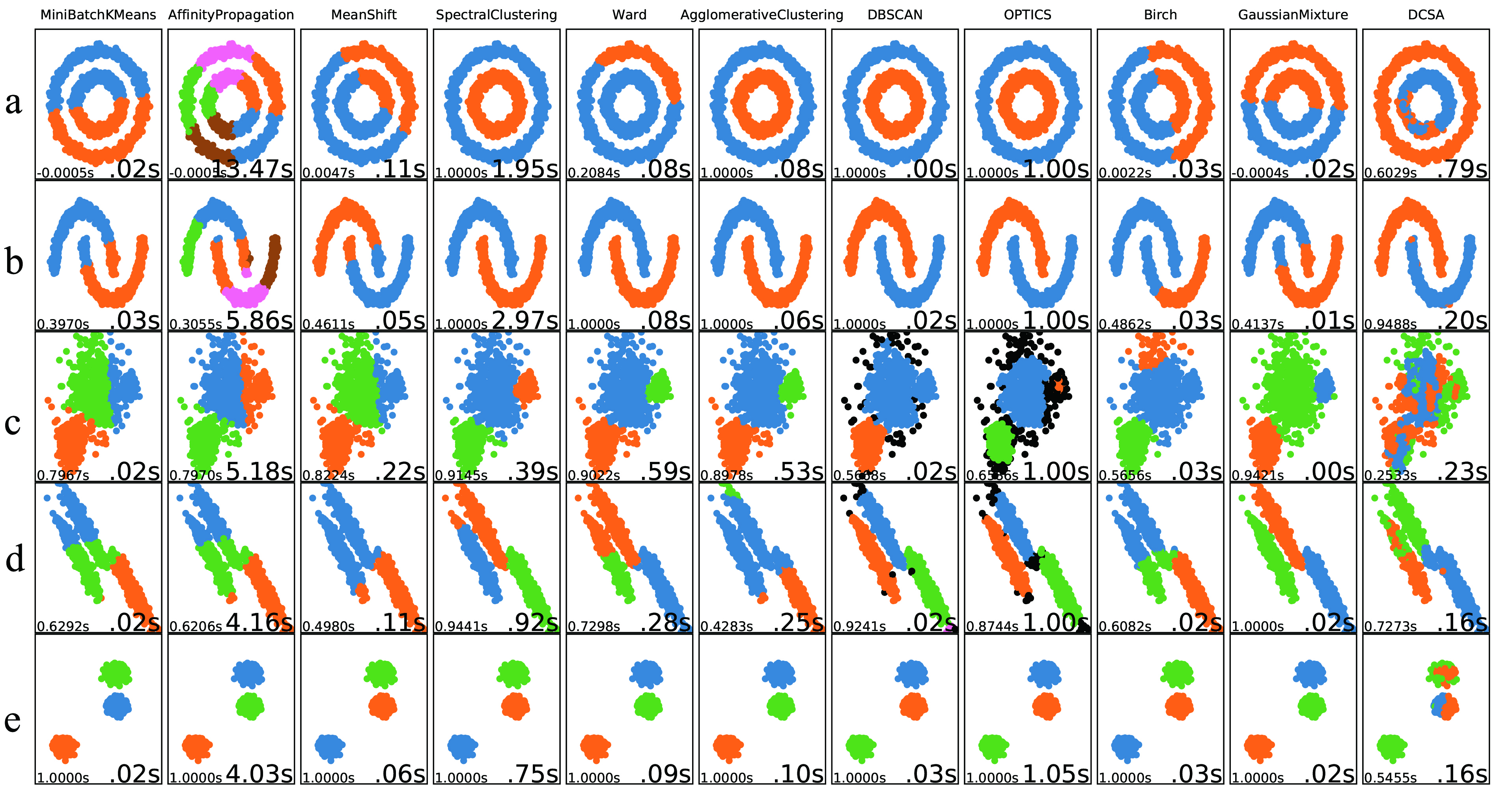
The DCSA algorithm in Figure 6 performs well on the dataset a, b, and d, all of which are with non-cluster structures. On the other hand, in the dataset c and e, especially the dataset c, the result shows that DCSA is invalid for low-dimensional data with fuzzy boundaries.
Table 1 shows the Adjusted Mutual Info(AMI) score of each algorithm. The algorithm numbers are: A1:MiniBatchK
Means, A2:AffinityPropagation, A3:MeanShift, A4:SpectralClustering, A5:Ward, A6:AgglomerativeClustering, A7:D
BSCAN, A8:OPTICS, A9:Birch, A10:GaussianMixture, A11:DCSA(with CUSUM-B).
.As shown in Table 1, the AMI score of DCSA is rank 7/11, and the best combined performer across the five datasets was SpectralClustering. Table 1 Scores of 11 algorithms on 5 generated datasets A1 A2 A3 A4 A5 A6 A7 A8 A9 A10 A11 0 0 0.005 1 0.208 1 1 1 0.002 0 0.603 0.397 0.305 0.461 1 1 1 1 1 0.486 0.413 0.949 0.796 0.797 0.822 0.914 0.902 0.898 0.566 0.656 0.565 0.9421 0.259 0.629 0.621 0.498 0.944 0.73 0.4283 0.9241 0.874 0.608 1 0.727 1 1 1 1 1 1 1 1 1 1 0.546 0.564:8 0.545:10 0.557:9 0.972:1 0.768:5 0.865:4 0.898:3 0.906:2 0.532:11 0.671:6 0.617:7
4.1.2 High dimensional test
We Manually Generated a 4-class Datasets (MGD) with 3000 instances and 60 attributes. After applying DCSA to MGD, the results are shown in Figure 7.
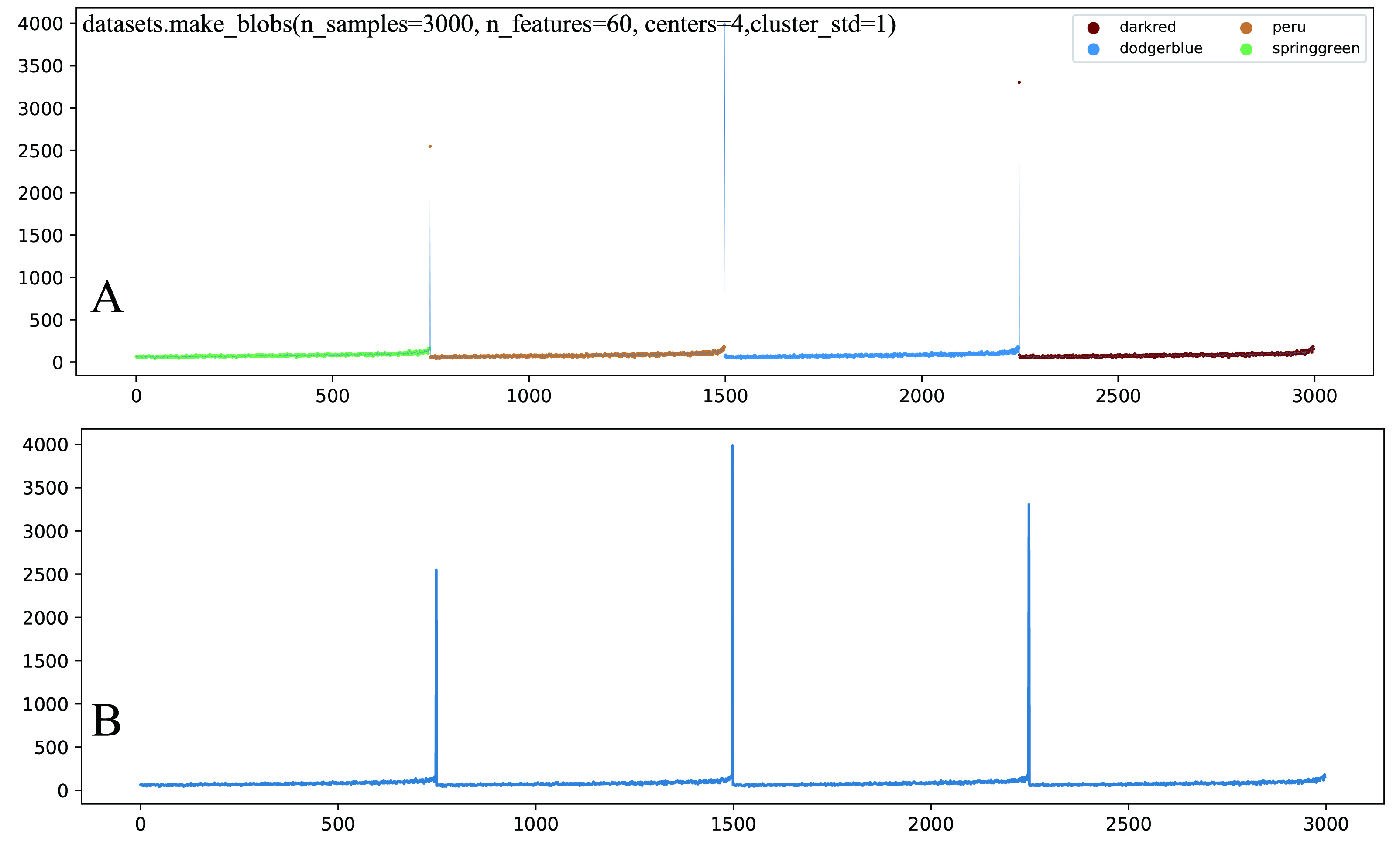
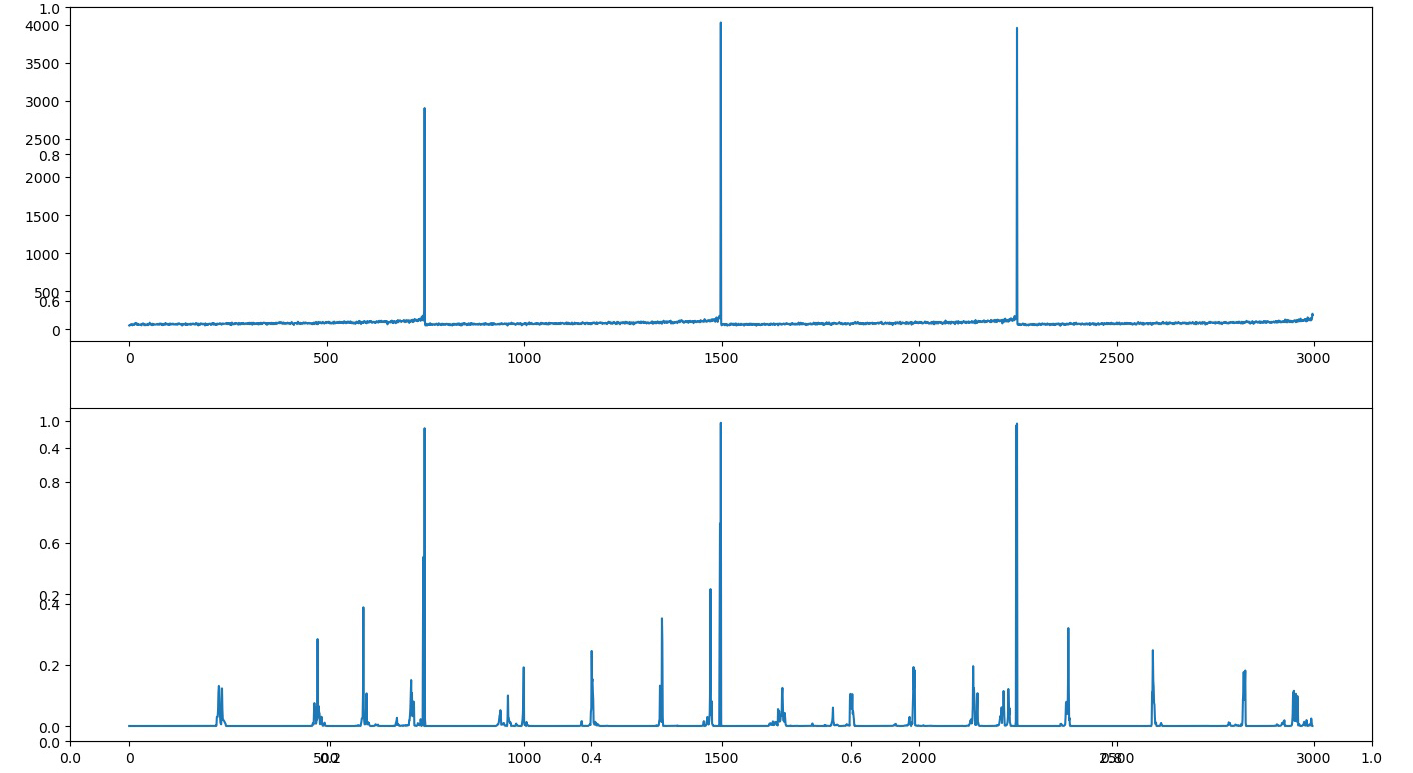
Figure 7B is the sequence generated by DCSA, and its coloring results in Figure 7A shows that the DCSA divides the different classes into separate fragments, of which each fragment delivers an upward trend. It is indicated that this phenomenon is a feature of the DCSA sequence.Then we use BCD to analyze the sequence, and the result is shown in Figure 8. The point where the probability is close to 1 is the correct cutoff point of the sequence.
The MGD dataset with isolated clustering structure are ideal, and rarely shown in real circumstances, and hence we need to further explore the performance of our algorithm with real-world dataset.
4.2 Real-world data experiment
In this section, DCSA is applied to the data set from UCI[1]&KEEL[27, 28], see the result in Table2 for the details.
| Table 2 | |||||||||
| Real world dataset experiment | |||||||||
| Records | Attribute | Cluster | Distribution | Area | Source | ||||
| 1797 | 64 | 10 |
|
Graphic | UCI | ||||
| 683 | 9 | 2 | 444/239 | Medical | KEEL | ||||
| 351 | 34 | 2 | 225/126 | Engineering | KEEL | ||||
| 358 | 34 | 6 | 111/60/71/48/48/20 | Medical | UCI | ||||
| 10092 | 16 | 10 |
|
Graphic | KEEL | ||||
| 801 | 20531 | 4 | 135/141/300/146/78 | Life | UCI | ||||
In the previous section, The Spectral Clustering is the algorithm with the highest overall performance, and Kmeans is the most efficient clustering algorithm. At the end of this section, will comparing DCSA with these two algorithms through AMI score.
4.2.1 Digits dataset[29]
This high-dimensional data set has 1797 instances and 64-dimensional attributes. It comes from the field of image recognition and is composed of handwritten Arabic numerals from 0 to 9. As the first real-world data experiment, we used the method in section 3.3 to analyze the DCSA sequence.
BCD application
Figure 9 depicts the results of application effect of the DCSA sequence and BCD algorithm.
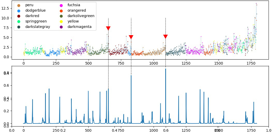
Except for the yellow and orange classes, most of other classes are concentrated on the same interval. In Figure 9 the red “" masks the corresponding position, where the correct point found by BCD algorithm, and the probability of the three point is greater than 0.5. However, no regularity can be observed at other points. It can be assumed that the BCD algorithm is relatively reliable at the position where the probability of the change point is close to 1.
CUSUM application
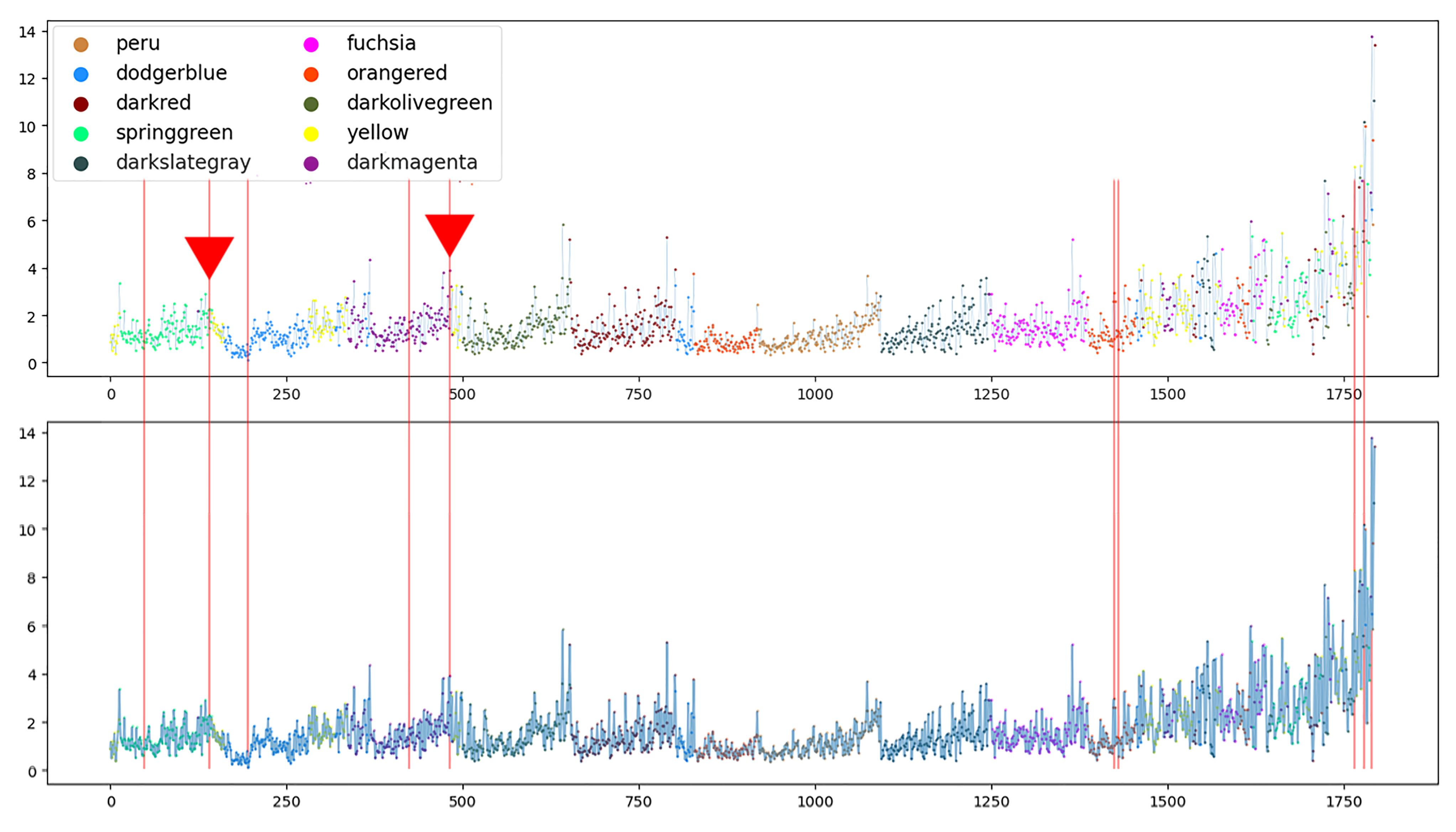
CUSUM requires two input parameters: Threshold and Accuracy. The threshold determines the maximum cumulative change, and the accuracy determines the degree of perception of subtle changes. Figure 10 shows the results of the DCSA sequence coloring and the CUSUM-A algorithm application effect().
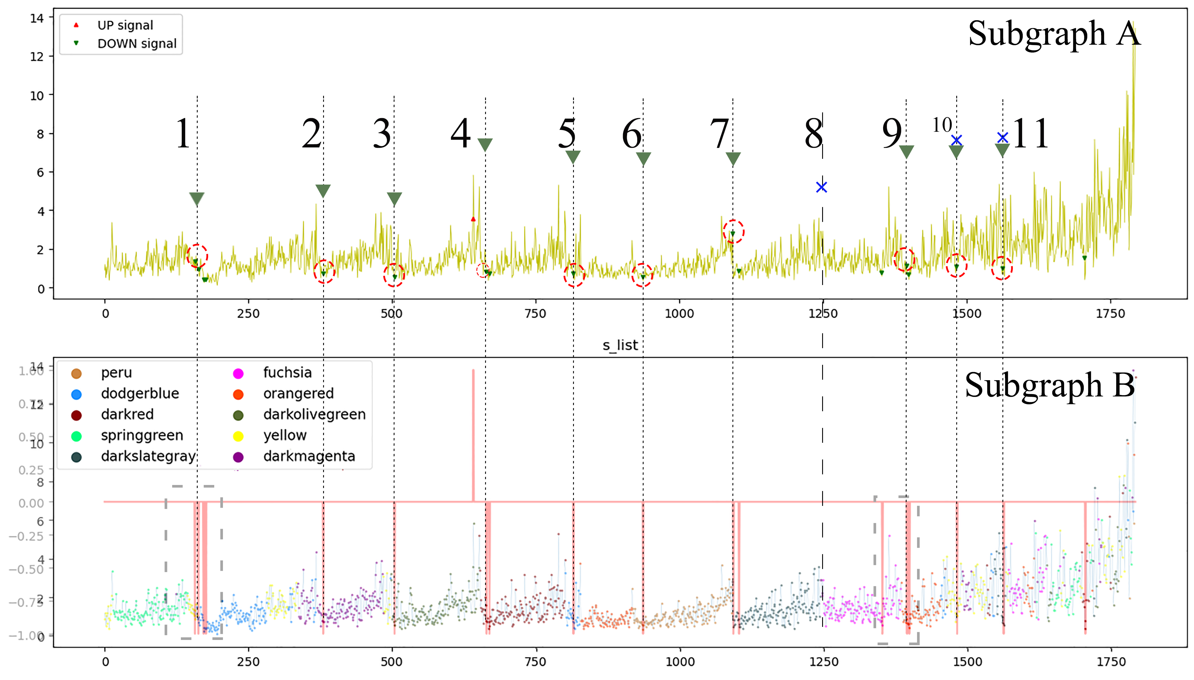
CUSUM-A Change Points are divided into “upper CP" and “lower CP". The red line in Figure 10B indicates the type and location of the change point. The mark “" illuminates the correct change point, and most of the “lower CP" just fall At the best cutting point except the place where marked “" by author. “" with “" means wrong change point.
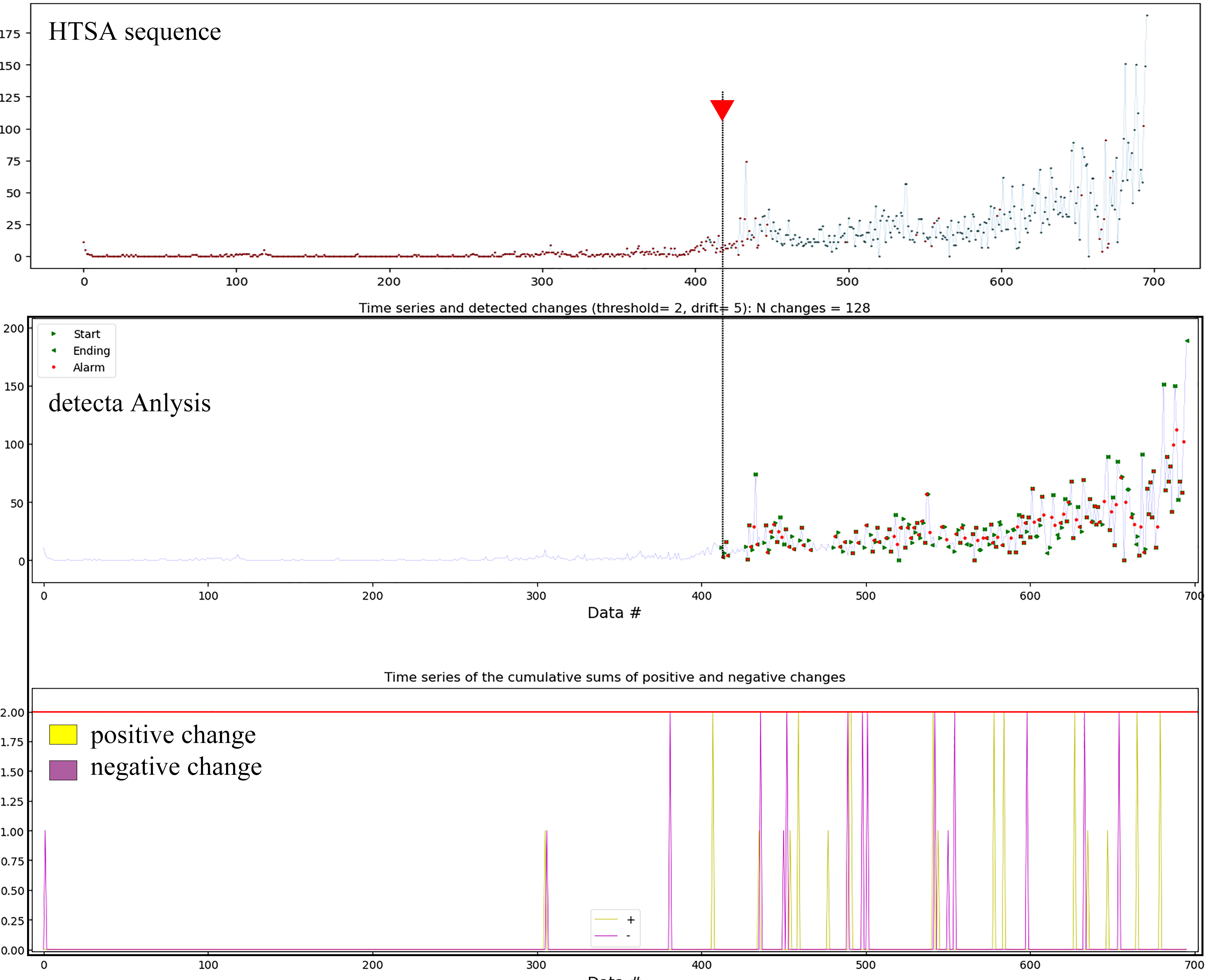
CUSUM-A is the algorithm edited by the author of this paper. On some specific data sets, CUSUM-B can get more detailed results, are shown in Figure 11.
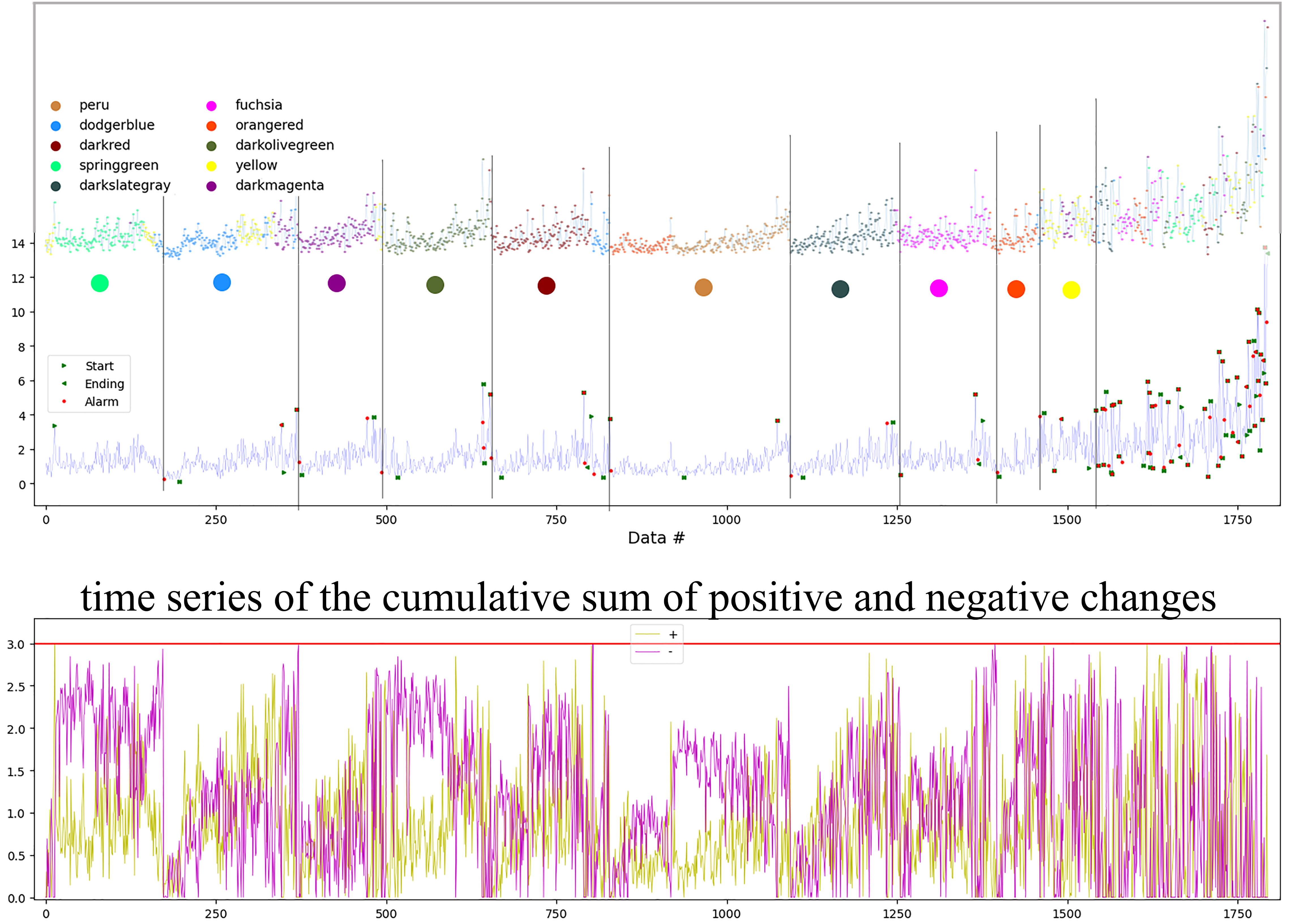
The red point (Alarm) in the figure is the change point. It is shown that the location of the change point is exactly the classification point.
CUSUM-B change point filtering:
When too many change points are detected locally, the results need to be further calculated: set the distance threshold between the existing change point and the next change point , When it is greater than , the new change point is adopted, otherwise the change point is discarded. Loop this process, and finally find all the change points of the division sequence.
ARIMA application
Figure 12 shows the calculation results of the ChangFinder function based on ARIMA.
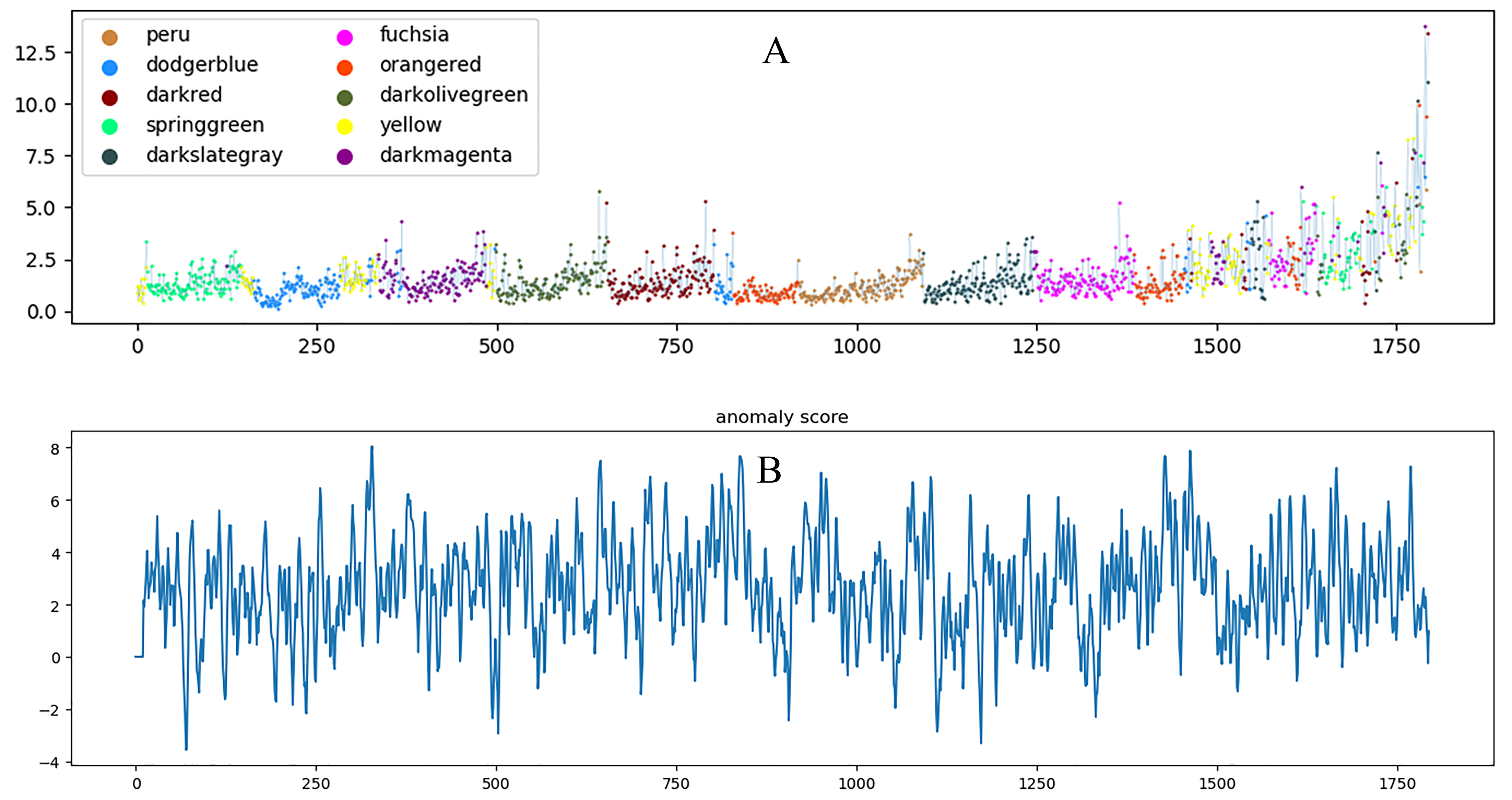
The analysis result of the ARIMA algorithm in Figure 12B shows that the ARIMA is not suitable for the DCSA sequence analysis.
JNBK application
The positions of the change point are shown in Figure 13.
Only some of the change points in Figure 13 are accurate, indicating the algorithm is not suitable for analysis the DCSA sequences.
The above experiments demonstrate that the CUSUM algorithm combined with the DCSA is effective on the digits data set. Other data experiments also support this conclusion. Except Wisconsin, the other datasets only show the sequence coloring results.
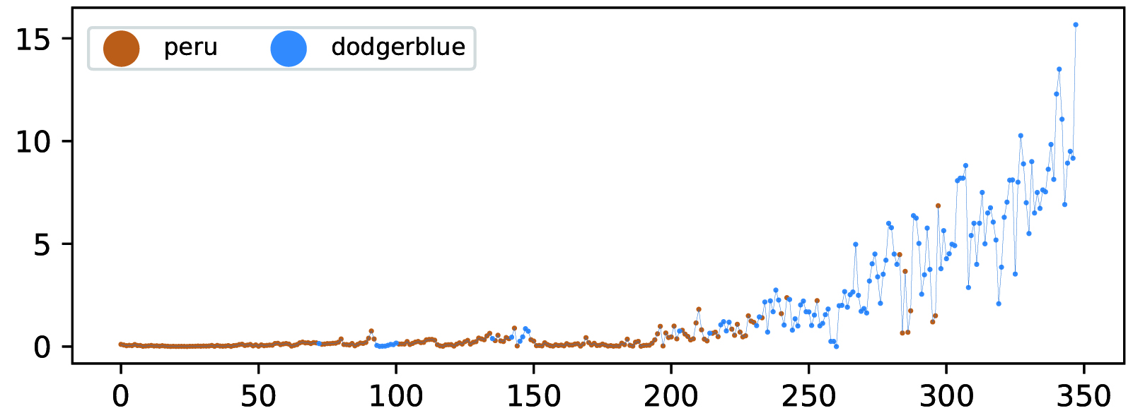
4.2.2 Wisconsin dataset
This medical data set contains cases of breast cancer surgery patients in a study conducted by the University of Wisconsin-Madison. It is an unbalanced low-dimensional data set. The goal of the experiment is to confirm whether the tumor detected by DCSA is benign or malignant. Figure 14 shows that the two categories are segmented correctly. The first one is relatively flat, while the latter shows an upward trend with fluctuations, and the connection between the two categories is relatively smooth. In this experiment, the CUSUM-B algorithm must be combined with the change point filtering in 4.2.1.2 to get the singal change point which is identified by the “” mark.
4.2.3 Ionosphere datasets
This data set is the classification data of ionospheric radar echo. This data set focuses on the performance of DCSA under the two-class high-dimensional imbalance. Figure 15 shows a small amount of misclassification.
4.2.4 Dermatology dataset
This data set distinguishes the types of skin diseases based on characteristics. The data set is high-dimensional and unbalanced. The application effect of DCSA is shown in Figure 16.
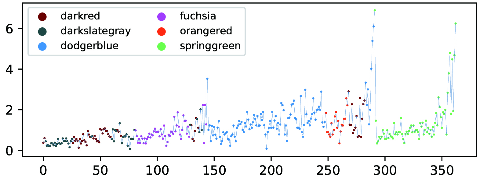
There are four categories in Figure 16 that are well divided. Darkred and darkslategray have some confusion.
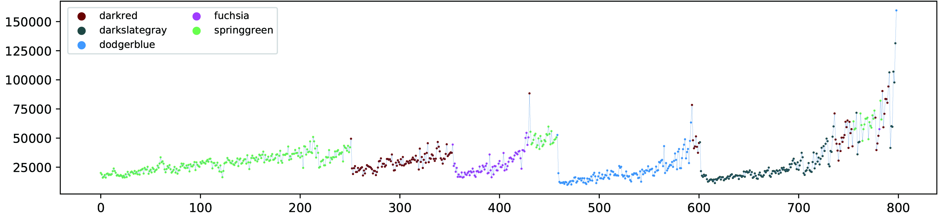
4.2.5 Penbased dataset
Digit database of 250 samples from 44 writers is high-dimensional and balanced, and has the largest number of samples in this paper (10092). The results are shown in Figure 17.
At the rear of the DCSA sequence of this dataset, various classes are mixed together. This should be caused by the overlapping of multiple classes in space.
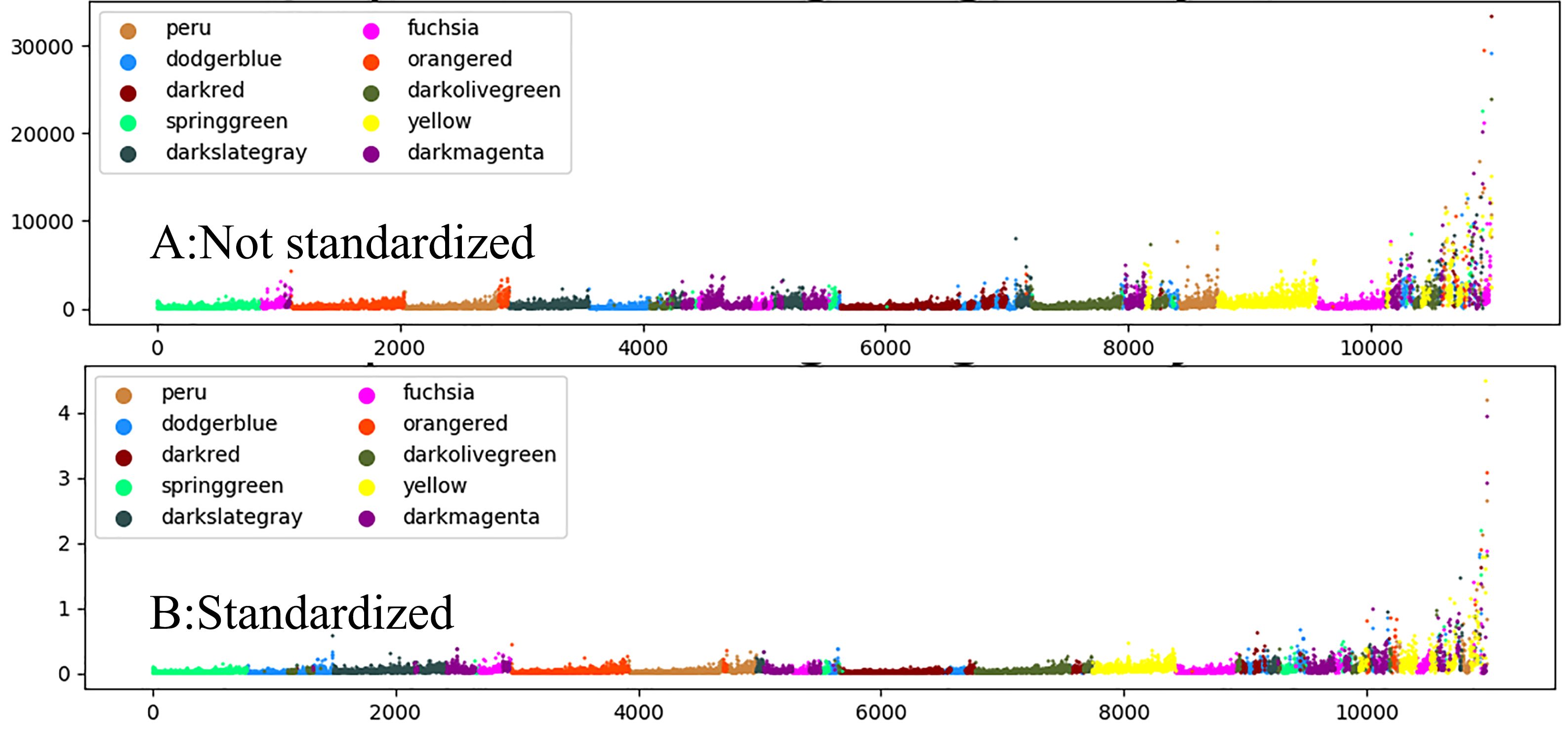
4.2.6 RNA-Seq dataset
This collection of data is part of the RNA-Seq (HiSeq) PANCAN data set, it is a random extraction of gene expressions of patients has different types of tumor: BRCA, KIRC, COAD, LUAD and PRAD. This data set is high-dimensional (the size reaches 20531), unbalanced and the size is larger than the number of samples. The algorithm performs better without standardizing the dataset. The classification results of DCSA algorithm is shown in Figure18.
Obviously, the DCSA application has achieved good results on this data set.
4.2.7 Algorithm evaluation and comparison
Table 3 compares the AMI scores of the three algorithms : Spectral Clustering, K-means, and DCSA.
In order to reproduce the results of the experiment, the parameters of spectral clustering are set as:
assign_labels="discretize",random_state=0.
| Table 3 | |||
| Algorithm evaluation and comparison | |||
| DCSA | K-means | SpectralClustering | |
| 0.614068803 | 0.736937078 | 0.74029209 | |
| 0.644677955 | 0.731813974 | 0.000934103 | |
| 0.415083449 | 0.130530901 | 0.027340228 | |
| 0.556677503 | 0.872912009 | 0.857759612 | |
| 0.534842473 | 0.665320729 | N/A | |
| 0.687214727 | 0.977097745 | -0.001459887 | |
| 0.575427485 | 0.685768739 | 0.270811024 | |
Spectral Clustering timed out on the Penbased dataset (more than 24 hours) and no results were output,When calculating the average score, we record it as 0.
5 Conclusions
Most data sets can be converted into numerical matrices after preprocessing. then the data has a feature space. The exploration of the feature space may reveal the latent patterns of data, DCSA is a new tools to do this. The experiment and visualization results on various types of data confirm the effectiveness of DCSA.
This version of DCSA application has experience requirements, because we need to choose a suitable sequence analysis algorithm, and these algorithms may need parameters such as thresholds. A stable sequence analysis method is an important prerequisite for the application of the DCSA. Subsequent work will further study the combination of sequence analysis and DCSA. In fact, if we don’t have prior knowledge, we can identify patterns through the periodic upward trend in the DCSA sequence chart. If the data has latent classes and the distance between classes is larger, this trend will become obvious, as we saw on Figure 18.
In addition, the DCSA algorithm also reveals some phenomena worthing further studing, such as why the same kind of data shows an upward trend in the DCSA sequence? In other words, why do experiments show that in most cases, when crossing classes, discovery factor(DF) go directly to the position with the highest density of the next class? The study of these phenomena may not only help us improve DCSA, but also give us a deeper understanding of the spatial distribution of data points.
References
- [1] Dheeru Dua and E Karra Taniskidou. Uci machine learning repository [http://archive. ics. uci. edu/ml]. irvine, ca: University of california. School of Information and Computer Science, 2017.
- [2] Dana Angluin and Leslie G Valiant. Fast probabilistic algorithms for hamiltonian circuits and matchings. Journal of Computer and system Sciences, 18(2):155–193, 1979.
- [3] Charles Bouveyron and Camille Brunet-Saumard. Model-based clustering of high-dimensional data: A review. Computational Statistics & Data Analysis, 71:52–78, 2014.
- [4] Guido Sanguinetti. Dimensionality reduction of clustered data sets. IEEE Transactions on Pattern Analysis and Machine Intelligence, 30(3):535–540, 2008.
- [5] Peter J Bickel, Elizaveta Levina, et al. Covariance regularization by thresholding. The Annals of Statistics, 36(6):2577–2604, 2008.
- [6] Gilles Celeux and Gérard Govaert. Gaussian parsimonious clustering models. Pattern recognition, 28(5):781–793, 1995.
- [7] Lance Parsons, Ehtesham Haque, and Huan Liu. Subspace clustering for high dimensional data: a review. Acm Sigkdd Explorations Newsletter, 6(1):90–105, 2004.
- [8] Adrian E Raftery and Nema Dean. Variable selection for model-based clustering. Journal of the American Statistical Association, 101(473):168–178, 2006.
- [9] Frank Harary, Robert Zane Norman, and Dorwin Cartwright. Structural models: An introduction to the theory of directed graphs. Wiley, 1965.
- [10] Roger A Horn and Charles R Johnson. Matrix analysis. Cambridge university press, 2012.
- [11] Reza Parhizkar. Euclidean distance matrices. Technical report, EPFL, 2013.
- [12] Richard Bellman. A markovian decision process. Journal of mathematics and mechanics, pages 679–684, 1957.
- [13] Andrey Andreyevich Markov. Extension of the law of large numbers to dependent quantities. Izv. Fiz.-Matem. Obsch. Kazan Univ.(2nd Ser), 15:135–156, 1906.
- [14] Eugene Seneta. Markov and the creation of markov chains. In Markov Anniversary Meeting, pages 1–20. Citeseer, 2006.
- [15] Thomas Hofmann, Bernhard Schölkopf, and Alexander J Smola. Kernel methods in machine learning. The annals of statistics, pages 1171–1220, 2008.
- [16] Suad A Alasadi and Wesam S Bhaya. Review of data preprocessing techniques in data mining. Journal of Engineering and Applied Sciences, 12(16):4102–4107, 2017.
- [17] Yin-Wen Chang, Cho-Jui Hsieh, Kai-Wei Chang, Michael Ringgaard, and Chih-Jen Lin. Training and testing low-degree polynomial data mappings via linear svm. Journal of Machine Learning Research, 11(4), 2010.
- [18] Li Ai Guo and Qin Zheng. On-line segmentation of time-series data(in chinese). Journal of Software.
- [19] Xiang Xuan. Bayesian inference on change point problems. PhD thesis, University of British Columbia, 2007.
- [20] Paul Fearnhead. Exact and efficient bayesian inference for multiple changepoint problems. Statistics and computing, 16(2):203–213, 2006.
- [21] Ryan Prescott Adams and David JC MacKay. Bayesian online changepoint detection. arXiv preprint arXiv:0710.3742, 2007.
- [22] Xiang Xuan and Kevin Murphy. Modeling changing dependency structure in multivariate time series. In Proceedings of the 24th international conference on Machine learning, pages 1055–1062, 2007.
- [23] Douglas M Hawkins. A cusum for a scale parameter. Journal of Quality Technology, 13(4):228–231, 1981.
- [24] Douglas M Hawkins and David H Olwell. Cumulative sum charts and charting for quality improvement. Springer Science & Business Media, 2012.
- [25] Dimitros Asteriou and Stephen G Hall. Arima models and the box–jenkins methodology. Applied Econometrics, 2(2):265–286, 2011.
- [26] George F Jenks. The data model concept in statistical mapping. International yearbook of cartography, 7:186–190, 1967.
- [27] Jesús Alcalá-Fdez, Luciano Sanchez, Salvador Garcia, Maria Jose del Jesus, Sebastian Ventura, Josep Maria Garrell, José Otero, Cristóbal Romero, Jaume Bacardit, Victor M Rivas, et al. Keel: a software tool to assess evolutionary algorithms for data mining problems. Soft Computing, 13(3):307–318, 2009.
- [28] Jesús Alcalá-Fdez, Alberto Fernández, Julián Luengo, Joaquín Derrac, Salvador García, Luciano Sánchez, and Francisco Herrera. Keel data-mining software tool: data set repository, integration of algorithms and experimental analysis framework. Journal of Multiple-Valued Logic & Soft Computing, 17, 2011.
- [29] Fabian Pedregosa, Gaël Varoquaux, Alexandre Gramfort, Vincent Michel, Bertrand Thirion, Olivier Grisel, Mathieu Blondel, Peter Prettenhofer, Ron Weiss, Vincent Dubourg, et al. Scikit-learn: Machine learning in python. the Journal of machine Learning research, 12:2825–2830, 2011.