Sparse SPN: Depth Completion from Sparse Keypoints
Abstract
Our long term goal is to use image-based depth completion to quickly create 3D models from sparse point clouds, e.g. from SfM or SLAM. Much progress has been made in depth completion. However, most current works assume well distributed samples of known depth, e.g. Lidar or random uniform sampling, and perform poorly on uneven samples, such as from keypoints, due to the large unsampled regions. To address this problem, we extend CSPN with multiscale prediction and a dilated kernel, leading to much better completion of keypoint-sampled depth. We also show that a model trained on NYUv2 creates surprisingly good point clouds on ETH3D by completing sparse SfM points.
1 Introduction
Depth completion methods aim to produce a depth value for each pixel, given an RGB image and a sparse set of depth values. Sparse depths may come from depth sensors, such as Lidar, or feature-based reconstruction such as structure-from-motion (SfM) or simultaneous localization and mapping (SLAM). Completed depth maps are useful for many applications, including robotics grasping and navigation, novel view synthesis, photo editing, and augmented reality. Accurate and efficient completion is, therefore, an important area of research.
Existing works [35, 19, 2, 17, 3, 7, 36] focus on Lidar completion, where sparse depth is distributed roughly uniformly over the image. For experiments on indoor scenes, these methods simulate sparse depth by uniform random sampling from ground truth depth. In both cases, each local neighborhood is likely to contain at least one sparse depth point, so existing works can be seen as RGB-guided interpolation of depth within a limited spatial extent.
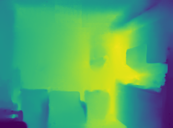
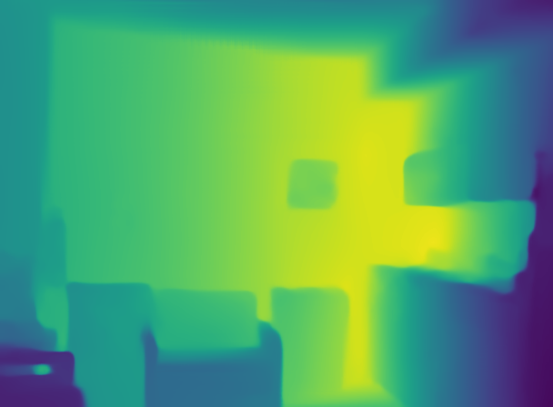
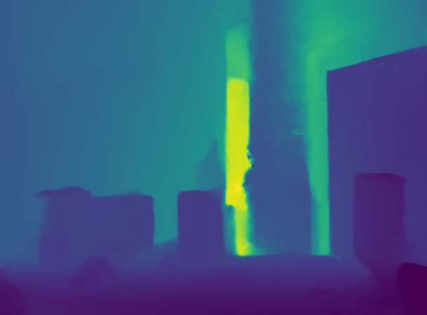
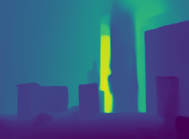
 |
 |
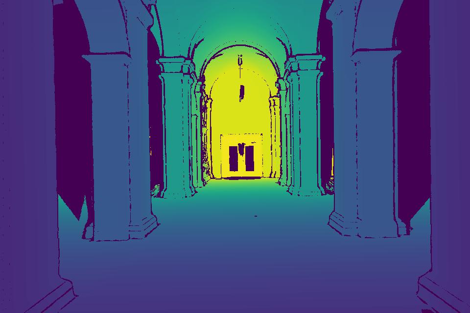
| (a) RGB & S. Depth | (b) Ground Truth |
 |
 |
| (c) CSPN [2] | (d) Ours |
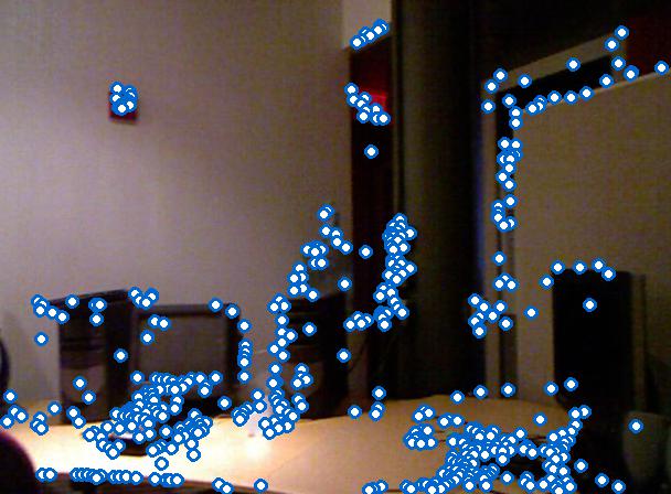
Our work focuses on completing depth from sparse keypoint-based reconstruction, e.g. obtained by SfM or SLAM with SIFT [14] or FAST [21] features. In such cases, sparse depth is typically densely distributed in textured regions, while unavailable in large untextured regions. We find that currently best-performing methods are unable to accurately propagate and extrapolate depth to these large unsampled regions (Fig. 1). We show that training on keypoint-sampled depth values significantly improves inference in keypoint-based depth while retaining similar performance in completion from uniformly sampled depth. Further, our proposed SSPN (Sparse Spatial Propagation Network) algorithm builds on Convolutional Spatial Propagation Network (CSPN) [2], which learns to propagate depth values using a data-sensitive affinity matrix, by introducing coarse-to-fine prediction, dilating the kernel [34, 4], and adding guidance from predicted surface normals. Together, these greatly increase the network’s ability for long-range depth propagation.
In experiments, we train our depth completion model on RGBD images from NYU v2 dataset [26] based on depth values from SIFT [14] detected keypoint locations. Evaluating on NYU v2 test data, we show that our SSPN model outperforms CSPN [2] and NLSPN [17] methods in this setting. We further demonstrate completion of sparse depth points by applying our model trained on NYU v2 to noisy sparse points obtained using SfM on the ETH3D dataset [24], again substantially outperforming other spatial propagation networks for depth completion. We fuse the depth maps to obtain 3D point clouds and show that our method yields similar scores to the GIPUMA [4] MVS algorithm, though with a very different accuracy-completion trade-off. Our ablation study indicates that dilation and coarse-to-fine modifications have little benefit on their own but jointly lead to large improvement, which made the discovery of this improvement non-obvious. We also find that models trained on keypoint sampled depth are generally applicable, while those trained on uniformly sampled depth perform poorly in other sampling scenarios. Finally, we compare under the experimental setups described by previous works for visual SLAM completion on Azure Kinect Dataset [22], low resolution uniformly sampled depth completion on NYU v2 and Lidar depth completion on KITTI [5], where our method is competitive with state-of-the-art.
Our main contributions are to investigate and improve depth completion from unevenly sampled points (keypoints), including:
-
•
Propose dilated kernel, coarse-to-fine architecture, and surface normal guidance for SPN that improve depth completion, in part by increasing the receptive field and providing geometry guidance for propagation
-
•
Evaluate depth completion from keypoint positions, demonstrating that existing SPN-based depth completion methods are not suited to unevenly sampled points, that our proposed contributions yield significant improvements, and that efficient generation of dense point clouds from sparse SfM points is possible.
2 Related Works
Approaches to Depth Completion: Depth completion aims to recover dense depth mapping given sparse depth values and an RGB image. Ma and Karaman [15], to our knowledge, are the first to apply deep learning to the problem. They use a CNN encoder-decoder to generate depth maps from RGB and sparse depth values, showing large improvements compared to prediction from RGB only. Application is also shown to Lidar completion and completion from sparse SLAM points, though the latter includes only one qualitative result. Experimenting on Lidar and simulated Lidar, Jaritz et al. [9] show that separately encoding RGB and sparse depth is helpful, with late stage fusion before the decoder. Zhang and Funkhauser [35] complete missing regions in sensor (e.g. Kinect) depth maps by predicting surface normals and boundaries and using them as constraints to solve for missing depth values. Xiong et al. [31] show the effectiveness of completion based on propagation using a Graph Neural Network (GNN). They also show that Poisson disc sampling of sparse depth enables better completion than uniformly random sampling, but this seems to assume that dense depth data is available at test time. Qiu et al. [19] and Xu et al. [33] generate surface normals and confidence maps and use them together with the RGB and sparse depths to complete depth maps from Lidar sensors. In a refinement stage, Xu et al. also incorporate a diffusion block and guidance map, which is conceptually similar to the spatial propagation networks discussed in the next subsection. Zhao et al. [36] introduce a co-attention guided graph propagation in encoder to enable pixels to capture useful observed contextual information more effectively, and uses symmetric gated fusion strategy to fuse the multi-modal contextual information efficiently, with application to Lidar and randomly sampled depth completion. Hu et al. [7] refine predictions from an encoder-decoder network with CSPN++ propagation [3]. Huynh et al. [8] explore depth completion with points from SfM in an RGBD indoor dataset by extracting multi-scale RGB and 3D sparse point features, but experiments do not include point cloud generation, and code is not available for comparison.
Motivated by depth completion from SLAM, Zhong et al. [37] propose a deep CCA method to recover missing depth values based on correlation between RGB features with known sparse depth values. Their experiments include completion from uniform, high-texture, and feature-based sampling, demonstrating slight improvement over CSPN. Another line of work [27, 16, 38] provides efficient solution that targets dense depth estimation on light-weight, embedded systems. These methods allows inference with small computation power, but at the cost of lower precision. Wong et al. learn to complete depth in an unsupervised manner based on photometric consistency [30] and extend to incorporate adaptive regularization [28] and camera calibration [29]. Sartipi et al. [22] use planar geometry and gravity estimation to augment the sparse depth to perform depth completion network. These approaches rely on creating planar prior, through triangulation [30] or surface normal estimation with masking [22]. When compared on broadly used depth completion benchmarks, such as KITTI [5] and NYU v2 [26], these approaches, which are based on UNet-style architectures, underperform recent SPN-based approaches, though some may benefit from additional information such as IMU sensors or calibration. Our approach extends the line of SPN approaches to achieve state-of-the-art on completion of non-uniformly sampled depth values, while learning from ground truth depth and not requiring additional information or priors beyond the RGB image and sparse depth.
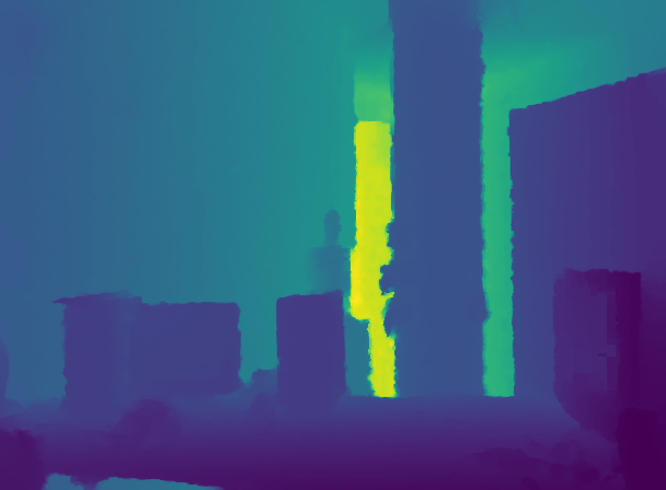
 |
 |
 |
 |
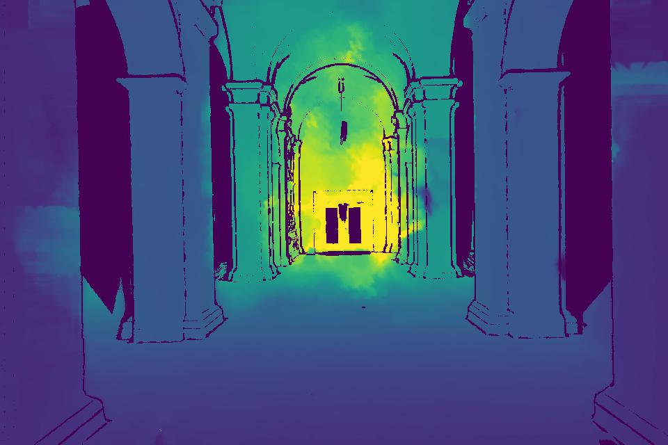
| (a) SPN[13] | (b) CSPN[2] | (c) NLSPN[17] | (d) Ours |
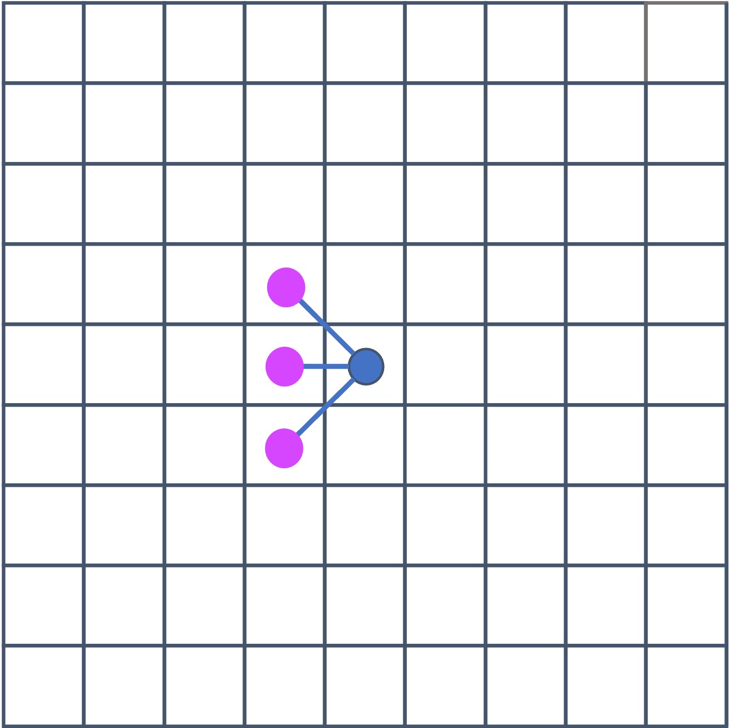
Spatial Propagation Networks: Liu et al.[13] propose spatial propagation networks (SPN). These networks learn to predict affinity matrices that encode pairwise similarities, and use them to aggregate information through row-wise and column-wise propagation. To reduce the memory and time cost, SPN uses a three-way connection, which allows each pixel to receive information from three neighboring pixels in each propagation step. Since SPN cannot be fully parallelized, Cheng et al. [2] propose a convolutional version of spatial propagation called CSPN, in which each pixel’s value is iteratively updated based on the neighborhood values from the previous iteration. CSPN is applied to depth completion, with the affinity matrix predicted by the RGB image used to propagate sparse depth values. Cheng et al.[3] further improve the effectiveness and efficiency of CSPN by learning adaptive convolutional kernel sizes and the number of iterations for the propagation. Park et al.[17] use deformable convolution to enable adaptive, potentially non-local neighborhoods as the basis for propagation and also introduce an affinity matrix normalization scheme, leading to state-of-the-art performance for completion from NYU v2 [26] random sampling. Lin et al.[12] apply attention to affinity values of different distance, achieving state-of-the-art performance for KITTI [5] depth completion benchmark.
We extend CSPN by introducing coarse-to-fine estimation with dilated kernels, which we show outperforms NLSPN and other methods for completion from keypoint-sampled depth.
3 Method
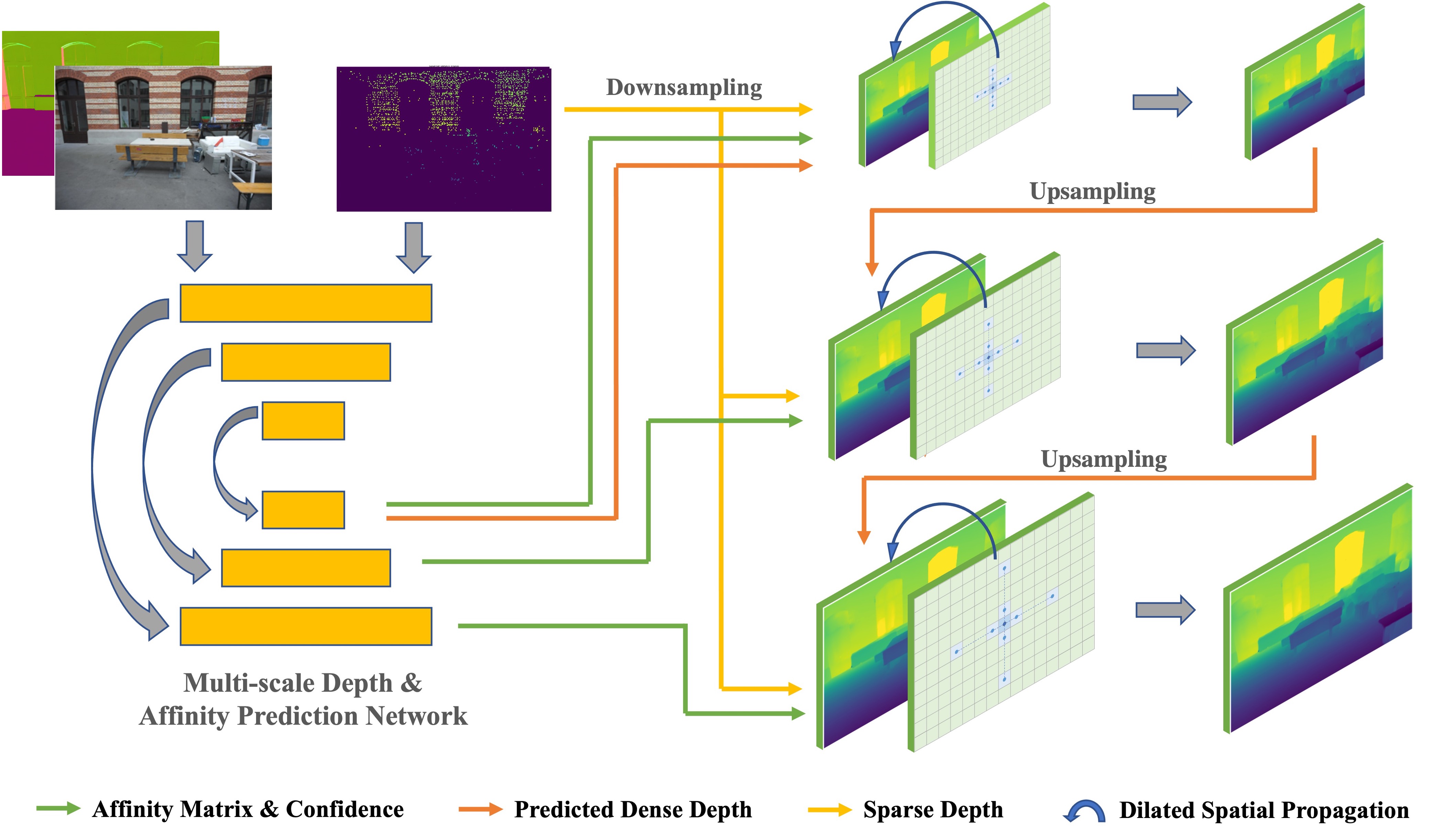
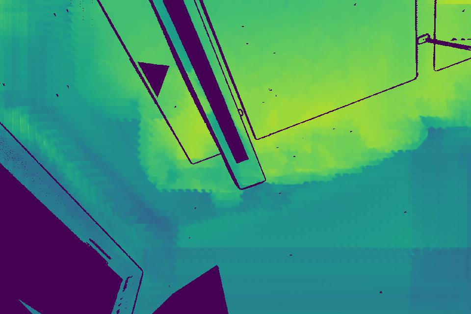
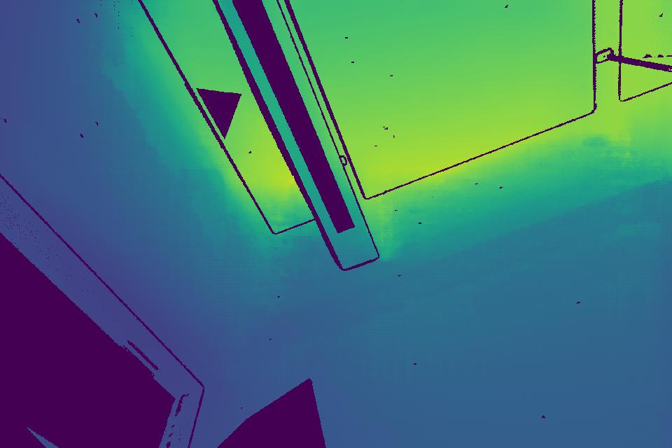
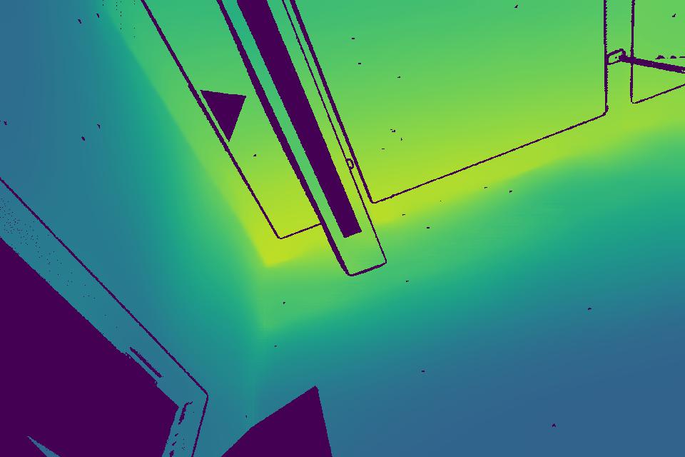
We extend the Convolutional Spatial Propagation Network [2] with a coarse-to-fine scheme, dilated propagation kernel, and surface normal guidance. Fig. 2 provides an overview of our method. Given an RGB image, sparse depth, and (optionally) predicted surface normals map, our network predicts the initial depth map at the lowest resolution, and predicts an affinity matrix and confidence map at each scale. Starting with the initial predicted depth, the depth is refined at each scale using spatial propagation with predicted affinity values and confidences and a dilated kernel and then upsampled.
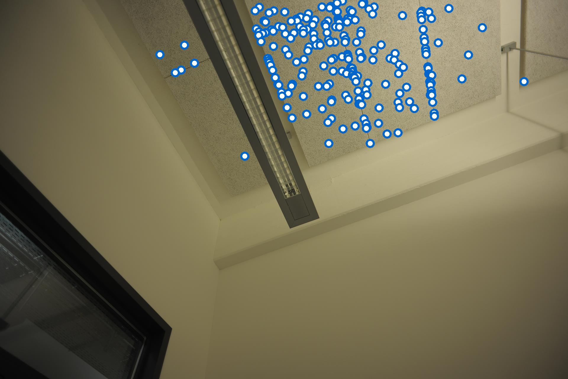
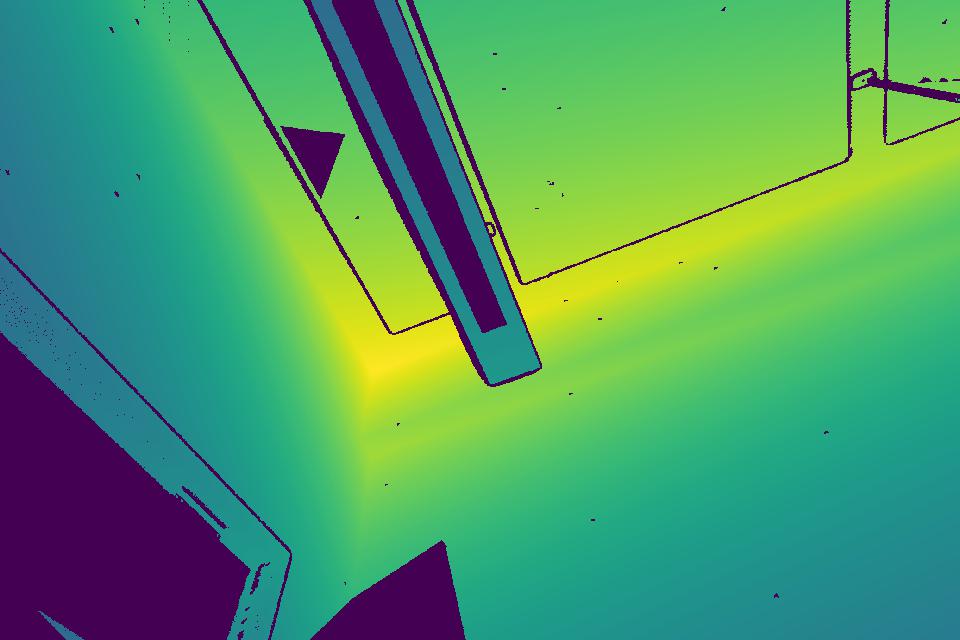
 |
 |
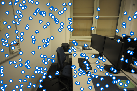 |
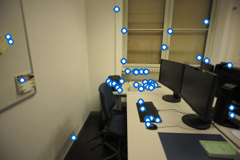
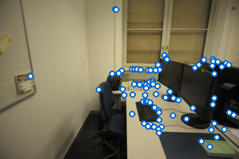
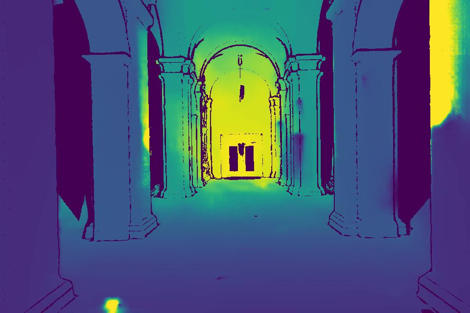
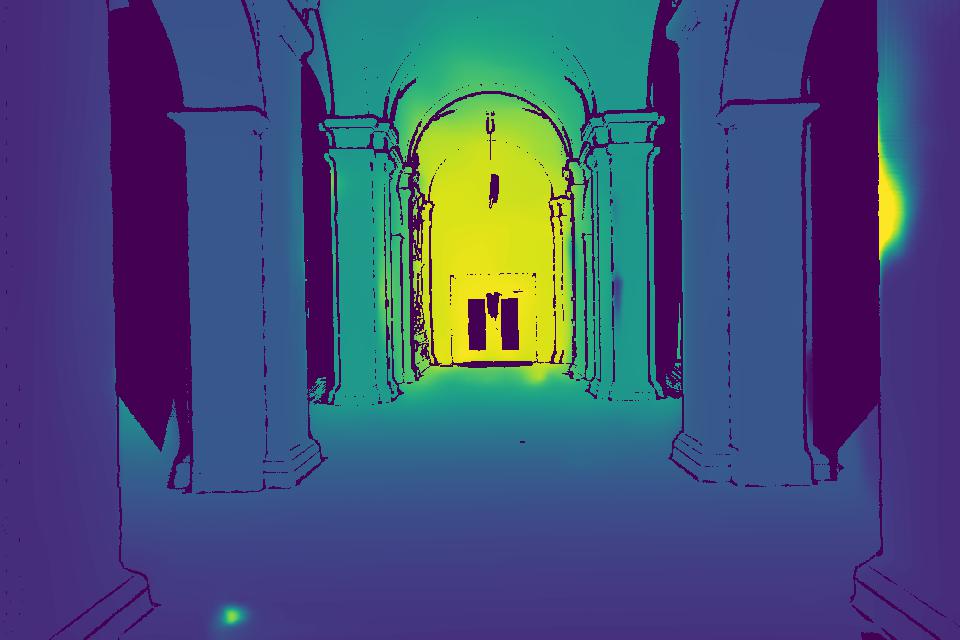
| (a) Sparse Points | (b) Keypoint | (c) Random |
3.1 Convolutional Spatial Propagation Networks
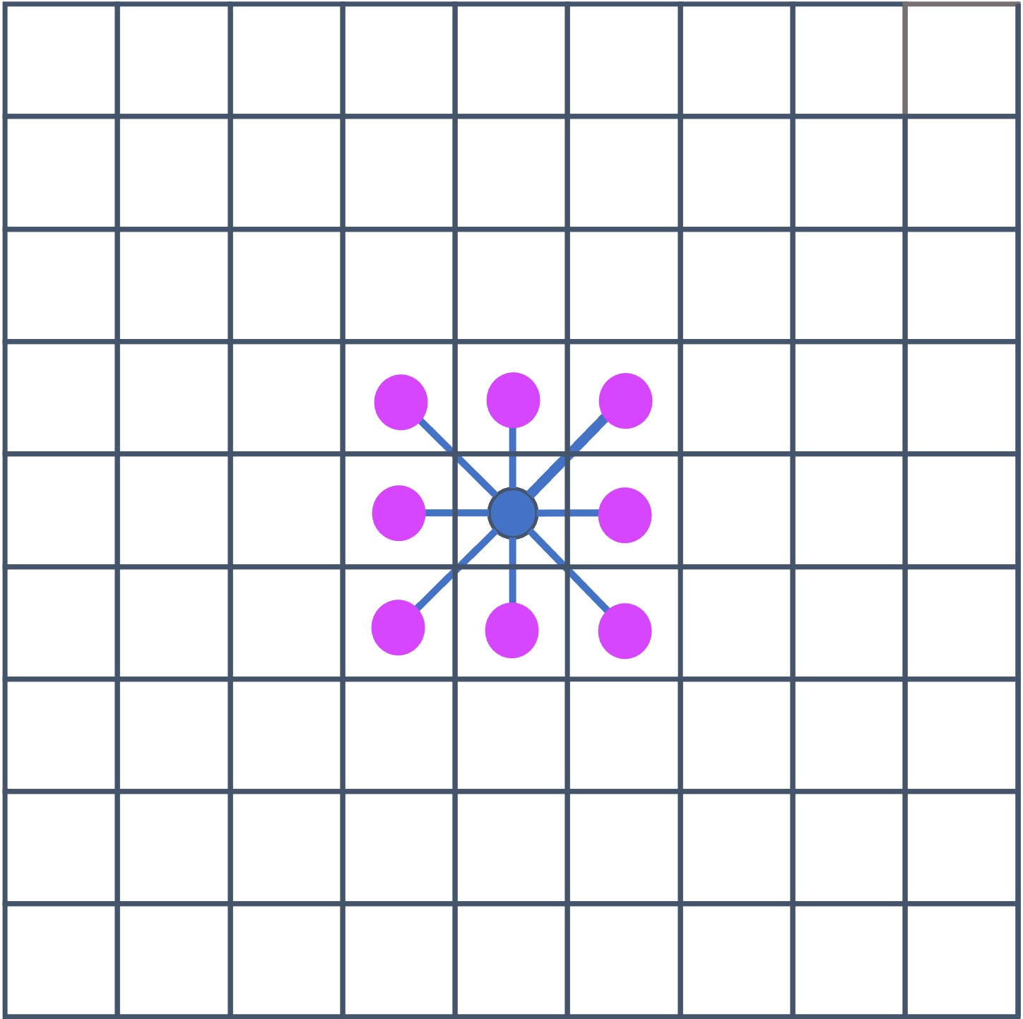
Spatial propagation networks (SPN) [13, 2, 17] learn to predict affinity values that indicate pairwise similarity between each pixel and its neighbors. The pairwise similarities are used to iteratively propagate the known values to the nearby unknown values, such as propagating sparsely distributed depth values to the rest of the image [2, 3, 17]. The original SPN [13] propagates along rows and columns. Convolutional Spatial Propagation Network (CSPN) [2] updates all pixels simultaneously using convolution operations, based on values and affinites of each pixel’s neighborhood.
For depth completion, CSPN takes image and the sparse depth map as input, and uses a U-Net [20] based CNN model to estimate an initial dense depth map and the affinity map , where denotes the number of neighbors. Formally, a single iteration of convolutional propagation can be defined as:
|
|
(1) |
where denotes the depth value at pixel coordinate (), denotes the set of neighboring pixel coordinates, denotes the value of input depth, denotes the weight of the center pixel, and denotes the affinity value between pixels and . The weights are normalized to sum to 1. After fixed number of iterations, CSPN yields the refined dense depth map. The network is trained using the mean-squared-error loss between the refined depth map and ground truth depth map.
In more recent work [17, 3], confidences for each input depth value and predicted pixel are estimated. Given per-pixel confidence map , per-input depth , and per-input depth confidence , spatial propagation using confidence can be defined as:
| (2) |
| (3) |
 |
 |
 |
 |
 |
|
 |
 |
 |
 |
| RGB & Sparse input | Ground Truth | CSPN[2] | NLSPN[17] | Ours |
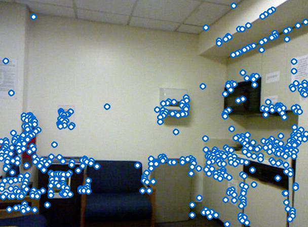
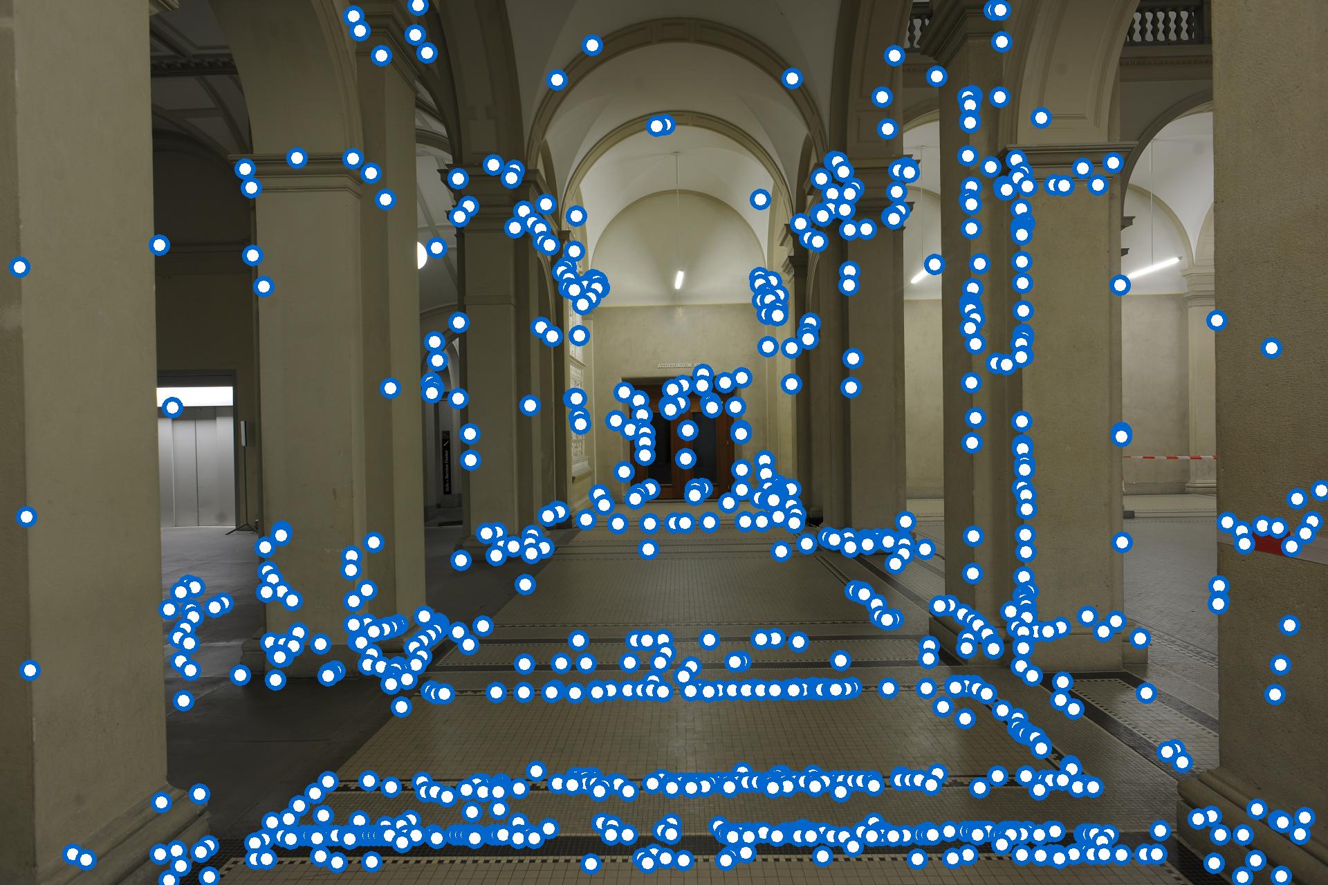
3.2 Keypoint Sampling
When training and testing based on RGBD images, many methods employ uniformly random sampling (each pixel is equally likely) to obtain sparse depth values, which results in known values that are scattered over the entire image. We investigate keypoint-based sampling, in which the sparse depth values are sampled at the positions of detected SIFT [14] keypoints. This simulates access to sparse depth values that may be available from keypoint triangulation, such as from SfM or SLAM. Our experiments show that models trained on RGBD images using keypoint-based sampling can be effectively applied complete depth images using the output of an SfM algorithm, even on significantly different image sets from training. SIFT detection is run on grayscale images, and the number of samples is capped. As shown in Fig. 4, the keypoints are densely distributed in highly textured regions while absent in other regions, which makes depth completion more difficult and particularly requires propagation over larger ranges, which motivates our Sparse Spatial Propagation Network (SSPN).
3.3 Sparse Spatial Propagation Network
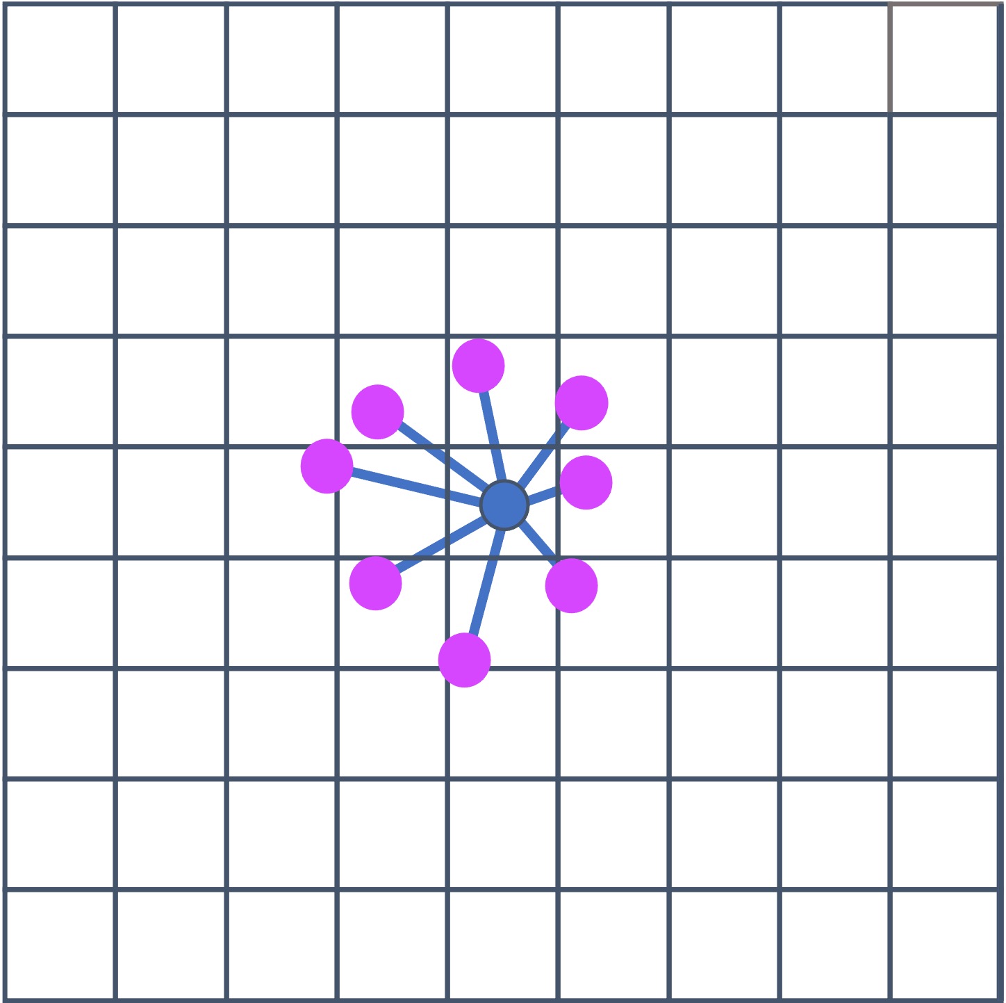
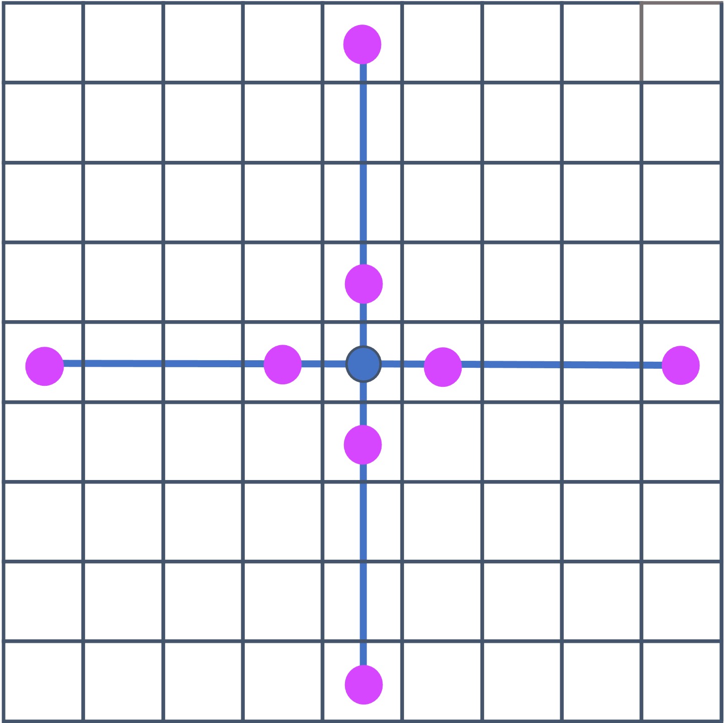
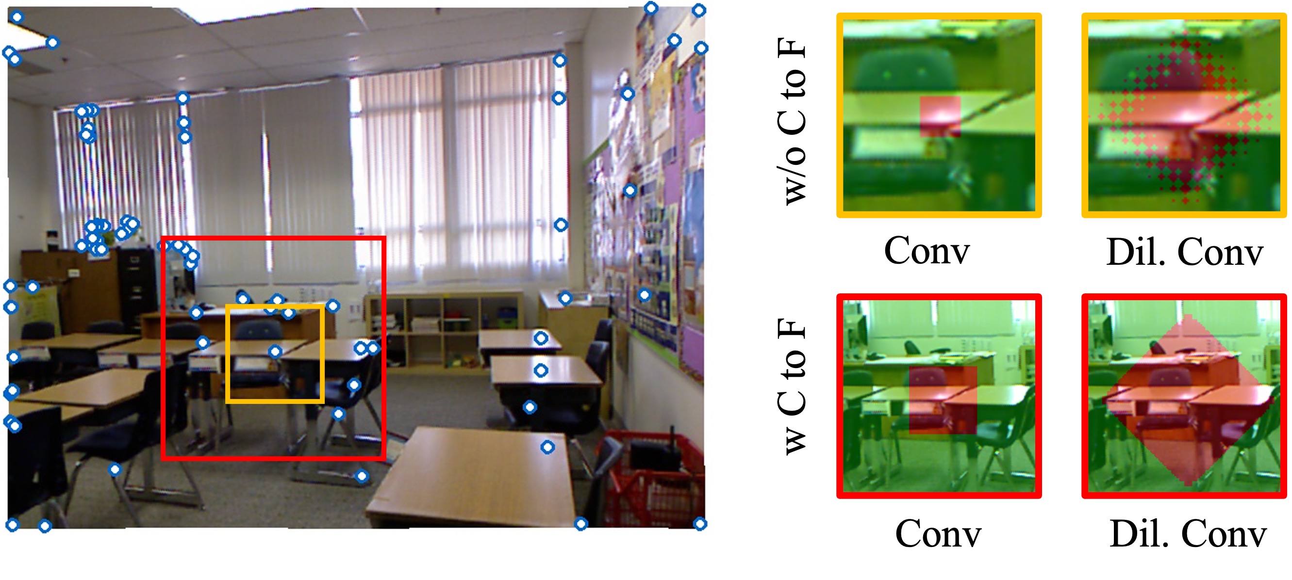
To expand the receptive field of propagation kernel, we propose two changes to the confidence-weighted CSPN architecture that was described in Sec. 3.1. First, we use coarse-to-fine scheme to extend the reach of the kernel by operating at low resolution in early iterations and refining into higher resolution. Next, we adopt the idea of diffusion based PatchMatch kernel [4] using dilated convolution, which provides a larger receptive field without increasing the number of iterations or computational cost. To provide a geometry guidance for the network, our network takes additional surface normal as input, which is estimated given color images with pretrained Omnidata network [10].
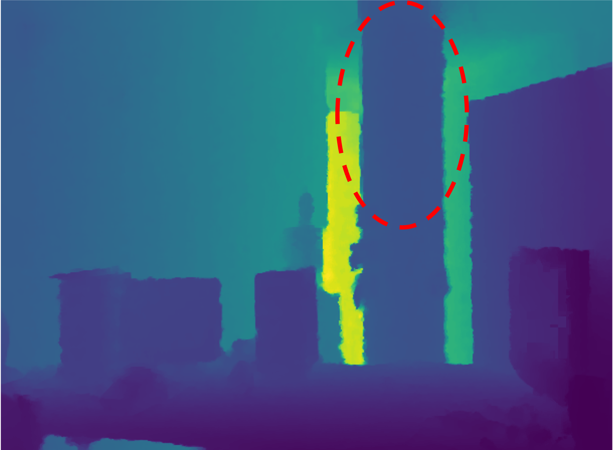
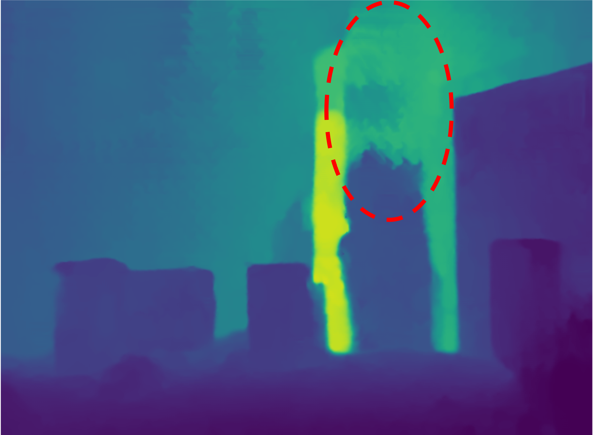
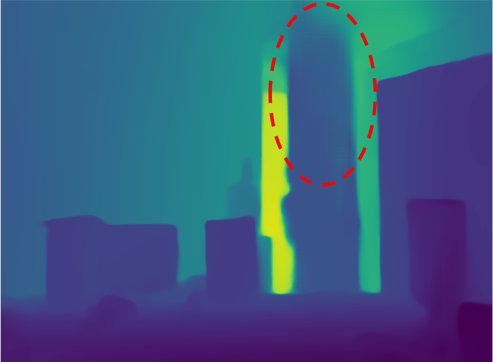
Fig. 2 provides an overview of the architecture. Similar to CSPN [2], we use U-Net [20] shaped model that receives an RGB image, surface normal image, and the corresponding sparse depth map and outputs an initial dense depth map at the coarsest scale and affinity and confidence maps at each scale. Within each scale, spatial propagation is iteratively performed using the dilated kernel shown in Fig. 3(d). After a fixed number of iterations, the current dense depth map is bilinearly upsampled, and spatial propagation continues at higher resolution. The kernel has a smaller dilation offset at coarser scales (see Sec. 3.5 for details). Fig. 5 visualizes the impact of each modification. By combining the coarse-to-fine architecture and the dilated kernel, the receptive field of the spatial propagation of our method (using 8 iterations over 4 scales), is increased by 93 times compared to the original CSPN method (using 24 iterations at the finest scale).
3.4 Loss Function
During the training, we apply a multi-scale loss between our prediction depth and ground truth:
| (4) |
where is the scale; is the predicted depth after propagation refinement in scale ; is the ground truth resized to the corresponding scale ; is the weight at scale , which is for lowest resolution, and increases by 1 for each finer scale. A smaller weight is used in low resolutions because the ground truth depth is less precise in low resolutions, due to downsampling. The use of multi-scale loss helps the network converge faster during training.
| Train | Test | Method | RMSE | REL | |||
|---|---|---|---|---|---|---|---|
| Key | Key | CSPN [2] | 0.220 | 0.043 | 55.3 | 78.3 | 88.9 |
| NLSPN [17] | 0.179 | 0.036 | 60.3 | 80.8 | 90.9 | ||
| Ours | 0.147 | 0.026 | 70.2 | 87.6 | 94.4 | ||
| Rnd | Rnd | CSPN [2] | 0.105 | 0.014 | 86.3 | 95.0 | 97.8 |
| NLSPN [17] | 0.098 | 0.012 | 88.6 | 95.6 | 98.0 | ||
| Ours | 0.102 | 0.013 | 86.5 | 94.6 | 97.6 | ||
| Key | Rnd | CSPN [2] | 0.131 | 0.020 | 71.1 | 92.3 | 97.1 |
| NLSPN [17] | 0.257 | 0.018 | 84.8 | 93.9 | 97.0 | ||
| Ours | 0.103 | 0.013 | 87.8 | 95.3 | 97.8 | ||
| Rnd | Key | CSPN [2] | 1.176 | 0.286 | 46.7 | 62.5 | 71.6 |
| NLSPN [17] | 0.330 | 0.083 | 53.0 | 70.5 | 80.9 | ||
| Ours | 0.406 | 0.078 | 51.3 | 69.0 | 78.9 |
 |
 |
 |
 |
 |
 |
 |
 |
 |
 |
| RGB & Sparse input | Ground Truth | CSPN[2] | NLSPN[17] | Ours |
3.5 Implementation Details
We use an encoder-decoder network for all experiments, with ResNet34 [6] as the encoder, and a decoder that contains two convolution layers in each scale. For all SPN methods without coarse-to-fine, 24 iterations of propagation are performed. For coarse-to-fine networks, 4 scales and 8 iterations per scale are used. We use a dilation size of 2 for dilated propagation in lowest scale, and increase by 1 for each finer scale. When sampling keypoint depth, we use the SIFT [1] detector of OpenCV [1].
During the training, we use Adam [11] optimization with the initial learning rate as 0.001 and decay as 0.85 each epoch step for all experiments. The training batch sizes are 6 for NYUv2 [26], and 12 for KITTI [5]. We train 30 epochs for all experiments. We implement our code using PyTorch [18], and use 1 NVIDIA A40 on KITTI [5] and 2 NVIDIA TITAN X (Pascal) on remaining for training and testing.
4 Experiments
Our main experimental questions:
- •
- •
- •
For completeness, we also compare to recent approaches using experimental setups from the literature in Sec. 4.4.
| 2cm: Completeness / Accuracy / F1 | 5cm: Completeness / Accuracy / F1 | ||||||
| Method | Resolution | Indoor | Outdoor | Combined | Indoor | Outdoor | Combined |
| Gipuma [4] | 2000x1332 | 24.6 / 89.3 / 35.8 | 25.3 / 83.2 / 37.1 | 24.9 / 86.5 / 36.4 | 34.0 / 96.2 / 47.1 | 36.7 / 95.5 / 51.7 | 35.2 / 95.9 / 49.2 |
| ACMM [32] | 3200x2130 | 68.5 / 92.5 / 78.1 | 72.7 / 88.6 / 79.7 | 70.4 / 90.7 / 78.9 | 78.4 / 96.4 / 86.1 | 83.9 / 96.2 / 89.5 | 80.9 / 96.3 / 87.7 |
| CSPN [2] | 960 x 640 | 34.9 / 20.0 / 25.1 | 24.9 / 18.9 / 20.3 | 30.3 / 19.5 / 22.9 | 51.9 / 38.2 / 43.4 | 40.1 / 36.2 / 37.0 | 46.5 / 37.2 / 40.4 |
| NLSPN [17] | 960 x 640 | 42.8 / 27.9 / 33.4 |
35.9 |
39.6 / 28.6 / 32.8 | 58.0 / 47.3 / 51.9 |
53.3 |
55.8 / 48.1 / 51.4 |
| Ours | 960 x 640 |
47.1 32.5 37.9 |
35.8 /
30.9 32.6 |
41.9 31.7 35.5 |
62.4 52.8 56.7 |
51.9 /
52.3 51.7 |
57.6 52.6 54.4 |
4.1 Completion from keypoints vs. uniformly random depth samples on NYU v2
NYU Depth V2 [26] consists of paired RGB images and dense depth maps collected from 464 different indoor scenes with a Microsoft Kinect. Following [15], the training sets are generated by sampling evenly from raw video sequences on training splits, and official test split of 654 densely labeled images are used for evaluation. All ground truth depth are obtained by filling missing values using original acquired raw depth. To exclude depth artifacts on borders, we center-crop the original frames to size . We sample 800 random samples and up to 800 SIFT [14] keypoints for each image. We use the same evaluation criteria used in [15], which evaluates the inferred depth Root-Mean-Squared Error (RMSE), Relative depth error (REL), and Percent Inlier metrics () where indicates the threshold of the inlier depth ratio.
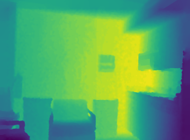
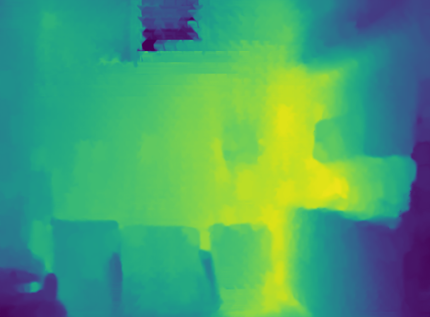
See Fig. 6 for qualitative results. In Table 1, we compare performance of CSPN [2], NLSPN [17], and our method on the NYU v2 dataset [26] under these two input settings, which we call “random” and “keypoint” samples for short.
-
•
When trained on random samples, CSPN and NLSPN perform well when tested on random samples () but perform very poorly when tested on keypoint samples ().
-
•
Compared to above, when trained on keypoint samples, CSPN and NLSPN performance reduces when tested on random samples () and improves moderately when tested on keypoint samples ().
-
•
When all methods are trained on keypoint samples, ours performs better than others when tested on random samples () or keypoint samples ().
These results indicate that prior methods have difficulty when sparse values are sampled from keypoints, while our method is more effective in this setting. Further, our method performs as well or better when training on keypoint samples than random samples in either test case, suggesting that keypoint sampling provides a more difficult training regime that leads to a more robust model.
4.2 Depth completion from sparse SfM points on ETH3D
ETH3D [24] is a challenging MVS dataset that provides stereo images, sparse point clouds generated by COLMAP [25], and ground truth depths captured by laser scanners. We use the training set of ETH3D, which contains 13 indoor and outdoor scenes with high-resolution images captured with sparsely sampled views, and evaluate three models trained on NYUv2 with keypoint samples, without fine-tuning. To test, we project the visible points (i.e., reconstructed tracks) from the sparse point cloud into each image to obtain the sparse depth map. These sparse depth values contain some outliers due to surface reflections and repeated structures, which makes the depth completion even more challenging. We downsample the images and the corresponding ground truth depth to (from original ), due to memory and runtime constraints.
We fuse the point clouds using the completed depths from each method by checking the absolute depth distance between each reference image with the source views following the fusion strategy of [4, 23]. We set the depth consistency threshold to 0.1 meters and number of required consistent views to 2.
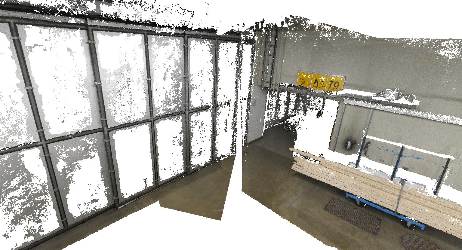
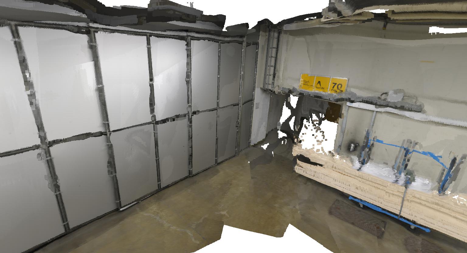
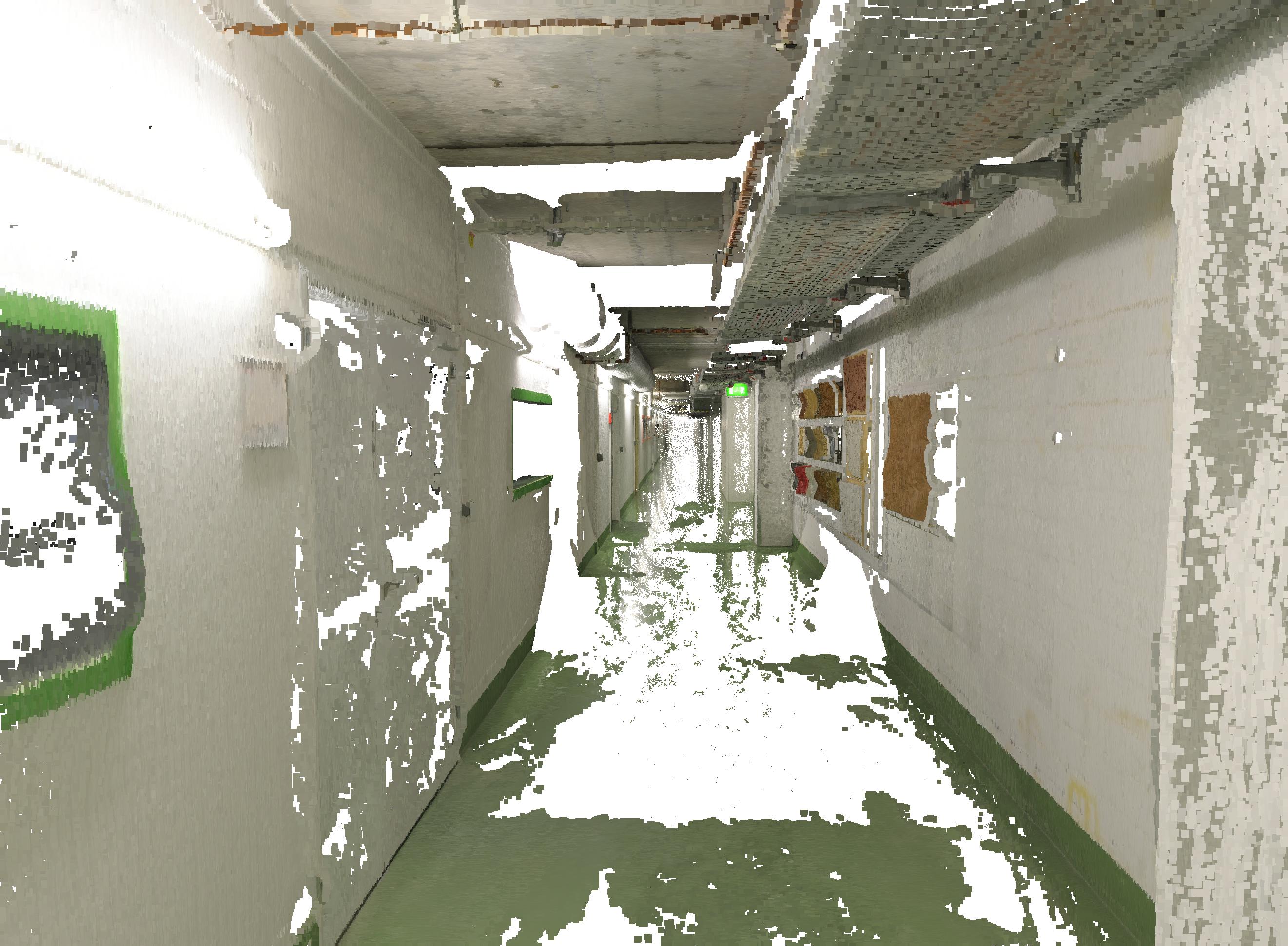
We compare the point clouds obtained using the spatial propagation methods to GIPUMA [4] and ACMM [32] MVS algorithms in Table 2 using standard metrics from ETH3D.
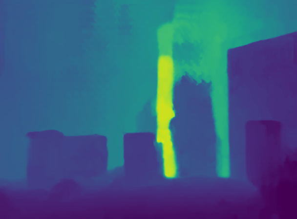
 |
 |
 |
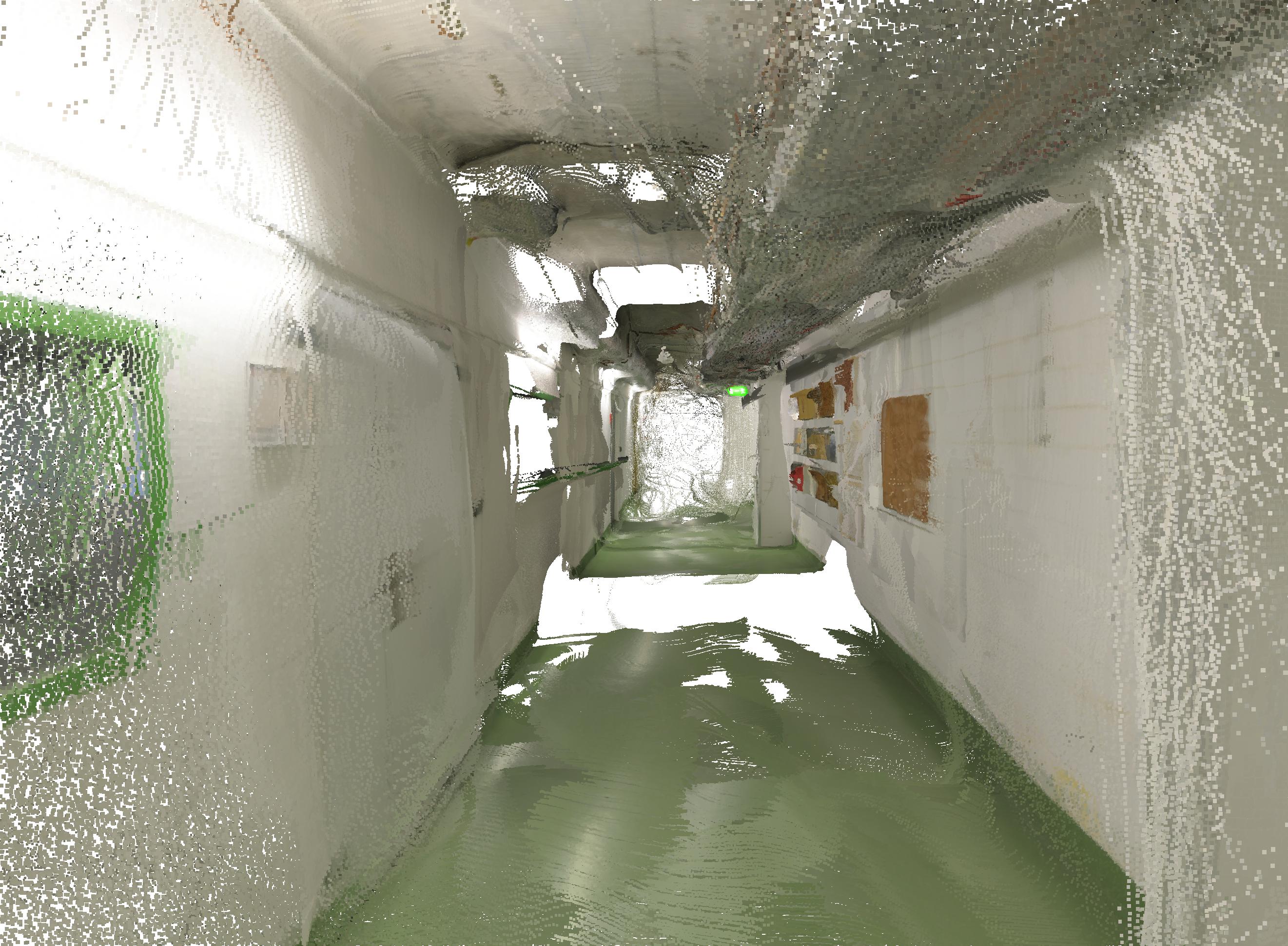 |
| ACMM [32] | Ours |
-
•
The point cloud from our fused single-view image completion achieves similar scores to GIPUMA MVS, with higher completion but lower accuracy.
-
•
For combined 2cm and 5cm F1-score, our method (35.5, 54.5) outperforms CSPN (22.9, 40.4) and NLSPN (32.8, 51.4), with a significant improvement on indoor scenes.
Considering Fig. 7, we see that our method is more robust to incorrect sparse depths and better completes low-texture regions such as walls and pillars. Fig. 8 compares the fused point cloud of our method to state-of-the-art MVS algorithm ACMM [32]. Though not as accurate as ACMM, our point clouds are more complete in textureless areas. These results show the promise of depth completion as an efficient way to generate depth point clouds from SfM or SLAM when MVS-level precision is not required, e.g. for photo tours and other visualizations.
| Method | RMSE | REL | ||||
| CSPN | 0.220 | 0.043 | 55.3 | 78.3 | 88.9 | 96.1 |
| w/ Dil. | 0.204 | 0.041 | 55.1 | 77.5 | 89.2 | 96.8 |
| w/ C. to F. | 0.200 | 0.040 | 57.4 | 78.9 | 89.7 | 96.9 |
| w/ Normals | 0.188 | 0.034 | 62.6 | 83.2 | 92.0 | 97.4 |
| w/ Conf. mask | 0.221 | 0.043 | 56.5 | 78.8 | 89.0 | 96.2 |
| w/ Dil.& w/ C. to F. | 0.159 | 0.031 | 64.8 | 84.4 | 92.9 | 98.1 |
| w/ All |
0.147 |
0.026 |
70.2 |
87.6 |
94.4 |
98.4 |
4.3 Ablation Studies
Table 3 evaluates the contribution of adding each of our proposed components to CSPN [2] on the NYUv2 dataset with the keypoint sampling. We find that coarse-to-fine inference on CSPN [2] (“w/ C. to F.”) improves the performance by a small margin, by 2.1% on and 0.003 on REL. Moreover, we show that while using dilated spatial propagation kernel alone does not improve over CSPN [2], differing only by 0.002 on REL and 0.016 on RMSE (“w/ Dil.”), the method achieves far better depth completion results when combined with the coarse-to-fine architecture, improving 9.5% over the CSPN [2] and 7.4% over CSPN with coarse-to-fine architecture (“w/ C. to F.”) on . We show that adding surface normal input achieves a significant improvement by 7.3% over CSPN [2] on because it provides geometry guidance for textureless plane areas. Confidence masks do not have much effect in NYU v2 experiments because the sparse depth samples are obtained from the same depth map used for ground truth.
Time/memory: CSPN [2], NLSPN [17], and our SSPN achieve frame rates of 4.8, 7.3, 4.9 FPS, with peak memory usage of 2443MB, 6985MB, 7179MB, respectively when testing on Quadro RTX 6000 on image resolutions of 960 x 640. Under the same setup, the pretrained Omnidata surface normal estimation model [10] achieves frame rate of 72.9 FPS, with peak memory usage of 4695 MB.
| Networks | REL | |||||
|---|---|---|---|---|---|---|
| CSPN (uniform sampling)∗ | 1.461 | 5.1 | 9.0 | 17.0 | 29.5 | 43.3 |
| DCN∗ | 0.814 | 15.1 | 28.7 | 57.9 | 82.2 | 91.5 |
| CSPN (keypoint sampling) | 0.714 | 17.6 | 32.2 | 60.5 | 83.8 | 93.7 |
| Ours |
0.166 |
24.3 |
43.6 |
75.3 |
92.5 |
96.8 |
4.4 Comparisons with existing works
We compare our method to existing depth completion methods [22, 19, 33, 2, 3, 17] on the visual SLAM, Lidar, and uniform sampled depth completion tasks, to provide a reference point of our method on the existing benchmarks. Specifically, we evaluate our method on the Azure Kinect dataset [22], KITTI depth completion benchmark [5] and resized NYUv2 dataset [26] with uniform sampled depth.
Results on Azure Kinect Dataset: Azure Kinect Dataset [22] contains 24 datasets in indoor areas. Each dataset comprises color, depth images, IMU measurements, and camera’s poses and triangulated feature positions processed by VI-SLAM. Following [22], we evaluate our network and CSPN [2], which are trained using keypoint sampling on NYUv2, on Azure under a resolution of 320 x 240. Table 4 presents the cross-dataset performance. Our method performs best, and CSPN [2] trained with keypoint achieves significant improvement over uniform sampling and performs better than DCN [22].
Benchmarking on KITTI Depth Completion: KITTI [5] contains over 93k RGB images and Lidar depth input, and ground truth depth. Following [17], we only use the bottom crop (1216 x 240) of the pairs for training. We use the criteria provided by the dataset [5], which includes RMSE, Invese RMSE (IRMSE), Mean-absolute Error (MAE) and Inverse MAE (IMAE). Table 5 presents the testing performance acquired from the official website. Our method is capable of achieving a similar IMAE result with state of the art.
| Method | RMSE | MAE | IRMSE | IMAE |
|---|---|---|---|---|
| CSPN [2] | 1019.64 | 279.46 | 2.93 | 1.15 |
| PENet [7] | 730.08 | 210.55 | 2.17 | 0.94 |
| CSPN++ [3] | 743.69 | 209.28 | 2.07 | 0.90 |
| NLSPN [17] | 741.68 | 199.59 | 1.99 | 0.84 |
| DYSPN [12] | 709.12 | 192.71 | 1.88 | 0.82 |
| Ours | 849.55 | 200.50 | 2.16 | 0.84 |
| Method | RMSE | REL | ||||
|---|---|---|---|---|---|---|
| DeepLiDAR [19] | 0.115 | 0.022 | - | - | - | 99.3 |
| DepthNormal [33] | 0.112 | 0.018 | - | - | - | 99.5 |
| ACMNet [36] | 0.105 | 0.015 | - | - | - | 99.4 |
| CSPN [2] | 0.117 | 0.016 | 83.4 | 93.5 | 97.0 | 99.2 |
| NLSPN [17] | 0.092 | 0.012 | 88.0 | 95.4 | 98.0 | 99.6 |
| Ours | 0.112 | 0.015 | 85.8 | 94.5 | 97.4 | 99.3 |
5 Limitations and Conclusion
We propose the Sparse Spatial Propagation Network (SSPN) that extends CSPN [2] with a coarse-to-fine architecture, dilated kernel, and surface normal inputs, increasing the range of propagation and leading to much better results for completion from keypoint samples. Our method also outperforms state-of-the-art NLSPN [17] when training from keypoint samples. Our point cloud fusion results indicate that depth completion methods may have applications for quickly creating dense point clouds from SfM or SLAM sparse point clouds. Further, it would be interesting to explore such methods as a refinement for MVS algorithms to improve completeness in textureless and reflective surfaces. The primary limitation of our method, as well as other depth completion methods, is precision, especially in comparison to MVS algorithms. Our multiscale network is also slightly slower than the other convolutional SPNs.
Acknowledgements This research is partially supported by NSF IIS 2020227, ONR N00014-21-1-2705, and a gift from Amazon. We thank Liwen Wu for the discussions and experiments of previous projects that helped shape SSPN.
References
- [1] Bradski, G.: The OpenCV Library. Dr. Dobb’s Journal of Software Tools (2000)
- [2] Cheng, X., Wang, P., Yang, R.: Learning depth with convolutional spatial propagation network. IEEE Transactions on Pattern Analysis and Machine Intelligence (TPAMI) (2020)
- [3] Cheng, X., Wang, P., Guan, C., Yang, R.: Cspn++: Learning context and resource aware convolutional spatial propagation networks for depth completion. In: Association for the Advancement of Artificial Intelligence(AAAI) (2020)
- [4] Galliani, S., Lasinger, K., Schindler, K.: Massively parallel multiview stereopsis by surface normal diffusion. In: IEEE International Conference on Computer Vision (ICCV) (2015)
- [5] Geiger, A., Lenz, P., Urtasun, R.: Are we ready for autonomous driving? the kitti vision benchmark suite. In: IEEE Conference on Computer Vision and Pattern Recognition (CVPR) (2012)
- [6] He, K., Zhang, X., Ren, S., Sun, J.: Deep residual learning for image recognition. IEEE Conference on Computer Vision and Pattern Recognition (CVPR) (2016)
- [7] Hu, M., Wang, S., Li, B., Ning, S., Fan, L., Gong, X.: Penet: Towards precise and efficient image guided depth completion. IEEE International Conference on Robotics and Automation (ICRA) (2021)
- [8] Huynh, L., Nguyen, P., Matas, J., Rahtu, E., Heikkila, J.: Boosting monocular depth estimation with lightweight 3d point fusion. IEEE International Conference on Computer Vision (ICCV) (2021)
- [9] Jaritz, M., de Charette, R., Wirbel, É., Perrotton, X., Nashashibi, F.: Sparse and dense data with cnns: Depth completion and semantic segmentation. International Conference on 3D Vision (3DV) (2018)
- [10] Kar, O.F., Yeo, T., Atanov, A., Zamir, A.: 3d common corruptions and data augmentation. In: IEEE Conference on Computer Vision and Pattern Recognition (CVPR) (2022)
- [11] Kingma, D.P., Ba, J.: Adam: A method for stochastic optimization. CoRR (2015)
- [12] Lin, Y.Q., Cheng, T., Zhong, Q., Zhou, W., Yang, H.: Dynamic spatial propagation network for depth completion. In: Association for the Advancement of Artificial Intelligence(AAAI) (2022)
- [13] Liu, S., Mello, S.D., Gu, J., Zhong, G., Yang, M.H., Kautz, J.: Learning affinity via spatial propagation networks. In: Advances in Neural Information Processing Systems (NeurIPS) (2017)
- [14] LoweDavid, G.: Distinctive image features from scale-invariant keypoints. International Journal of Computer Vision (IJCV) (2004)
- [15] Ma, F., Karaman, S.: Sparse-to-dense: Depth prediction from sparse depth samples and a single image. In: IEEE International Conference on Robotics and Automation (ICRA) (2018)
- [16] Merrill, N., Geneva, P., Huang, G.: Robust monocular visual-inertial depth completion for embedded systems. In: IEEE International Conference on Robotics and Automation (ICRA) (2021)
- [17] Park, J., Joo, K., Hu, Z., Liu, C.K., Kweon, I.: Non-local spatial propagation network for depth completion. In: European Conference on Computer Vision (ECCV) (2020)
- [18] Paszke, A., Gross, S., Massa, F., Lerer, A., Bradbury, J., Chanan, G., Killeen, T., Lin, Z., Gimelshein, N., Antiga, L., Desmaison, A., Kopf, A., Yang, E., DeVito, Z., Raison, M., Tejani, A., Chilamkurthy, S., Steiner, B., Fang, L., Bai, J., Chintala, S.: Pytorch: An imperative style, high-performance deep learning library. In: Advances in Neural Information Processing Systems (NeurIPS) (2019)
- [19] Qiu, J., Cui, Z., Zhang, Y., Zhang, X., Liu, S., Zeng, B., Pollefeys, M.: Deeplidar: Deep surface normal guided depth prediction for outdoor scene from sparse lidar data and single color image. In: IEEE Conference on Computer Vision and Pattern Recognition (CVPR) (2019)
- [20] Ronneberger, O., Fischer, P., Brox, T.: U-net: Convolutional networks for biomedical image segmentation. In: Medical Image Computing and Computer Assisted Intervention Society (2015)
- [21] Rosten, E., Drummond, T.: Machine learning for high-speed corner detection. In: European Conference on Computer Vision (ECCV) (2006)
- [22] Sartipi, K., Do, T., Ke, T., Vuong, K., Roumeliotis, S.I.: Deep depth estimation from visual-inertial slam. In: IEEE International Conference on Intelligent Robots and Systems (IROS) (2020)
- [23] Schönberger, J.L., Zheng, E., Frahm, J.M., Pollefeys, M.: Pixelwise view selection for unstructured multi-view stereo. In: European Conference on Computer Vision (ECCV) (2016)
- [24] Schöps, T., Schönberger, J.L., Galliani, S., Sattler, T., Schindler, K., Pollefeys, M., Geiger, A.: A multi-view stereo benchmark with high-resolution images and multi-camera videos. In: Conference on Computer Vision and Pattern Recognition (CVPR) (2017)
- [25] Schönberger, J.L., Frahm, J.: Structure-from-motion revisited. In: IEEE Conference on Computer Vision and Pattern Recognition (CVPR) (2016)
- [26] Silberman, N., Hoiem, D., Kohli, P., Fergus, R.: Indoor segmentation and support inference from rgbd images. In: European Conference on Computer Vision (ECCV) (2012)
- [27] Teixeira, L., Oswald, M.R., Pollefeys, M., Chli, M.: Aerial single-view depth completion with image-guided uncertainty estimation. IEEE Robotics and Automation Letters (RA-L) (2020)
- [28] Wong, A., Cicek, S., Soatto, S.: Learning topology from synthetic data for unsupervised depth completion. IEEE Robotics and Automation Letters (RA-L) (2021)
- [29] Wong, A., Soatto, S.: Unsupervised depth completion with calibrated backprojection layers. IEEE International Conference on Computer Vision (ICCV) (2021)
- [30] Wong, A., Fei, X., Tsuei, S., Soatto, S.: Unsupervised depth completion from visual inertial odometry. IEEE Robotics and Automation Letters (RA-L) (2020)
- [31] Xiong, X., Xiong, H., Xian, K., Zhao, C., Cao, Z., Li, X.: Sparse-to-dense depth completion revisited: Sampling strategy and graph construction. In: European Conference on Computer Vision (ECCV) (2020)
- [32] Xu, Q., Tao, W.: Multi-scale geometric consistency guided multi-view stereo. IEEE Conference on Computer Vision and Pattern Recognition (CVPR) (2019)
- [33] Xu, Y., Zhu, X., Shi, J., Zhang, G., Bao, H., Li, H.: Depth completion from sparse lidar data with depth-normal constraints. In: IEEE International Conference on Computer Vision (ICCV) (2019)
- [34] Yu, F., Koltun, V.: Multi-scale context aggregation by dilated convolutions. CoRR abs/1511.07122 (2016)
- [35] Zhang, Y., Funkhouser, T.: Deep depth completion of a single rgb-d image. In: IEEE Conference on Computer Vision and Pattern Recognition (CVPR) (2018)
- [36] Zhao, S., Gong, M., Fu, H., Tao, D.: Adaptive context-aware multi-modal network for depth completion. IEEE Transactions on Image Processing (TIP) (2021)
- [37] Zhong, Y., Wu, C.Y., You, S., Neumann, U.: Deep rgb-d canonical correlation analysis for sparse depth completion. Advances in Neural Information Processing Systems (NeurIPS) (2019)
- [38] Zuo, X., Merrill, N., Li, W., Liu, Y., Pollefeys, M., Huang, G.: Codevio: Visual-inertial odometry with learned optimizable dense depth. IEEE International Conference on Robotics and Automation (ICRA) (2021)