Prim-LAfD: A Framework to Learn and Adapt Primitive-Based Skills from Demonstrations for Insertion Tasks

Abstract

Learning generalizable insertion skills in a data-efficient manner has long been a challenge in the robot learning community. While the current state-of-the-art methods with reinforcement learning (RL) show promising performance in acquiring manipulation skills, the algorithms are data-hungry and hard to generalize. To overcome the issues, in this paper we present Prim-LAfD, a simple yet effective framework to learn and adapt primitive-based insertion skills from demonstrations. Prim-LAfD utilizes black-box function optimization to learn and adapt the primitive parameters leveraging prior experiences. Human demonstrations are modeled as dense rewards guiding parameter learning. We validate the effectiveness of the proposed method on eight peg-hole and connector-socket insertion tasks. The experimental results show that our proposed framework takes less than one hour to acquire the insertion skills and as few as fifteen minutes to adapt to an unseen insertion task on a physical robot.

1 Introduction

Reinforcement learning (RL) has been widely used to acquire robotic manipulation skills in recent years Gu et al. (2017); Kalashnikov et al. (2018). However, training an agent to perform certain tasks using RL is typically data-hungry and hard to generalize to novel tasks. This data-inefficiency problem significantly limits the adoption of RL on real robot systems, especially in real-world scenarios.

Motion primitives, due to their flexibility and reliability, serve as a popular skill representation in practical applications Johannsmeier et al. (2019); Voigt et al. (2020); Alt et al. (2021). A motion primitive is characterized by a desired trajectory generator and an exit condition. It is often realized by hybrid motion/force controllers, such as a Cartesian space impedance controller. Taking moving until contact as an example primitive, the robot compliantly moves towards the surface until the sensed force exceeds a pre-defined threshold; a formal definition of motion primitives is deferred to Section 3.2. Despite the light-weighted representation and wide generalizability of the primitives, their parameters are often task-dependent, and the tuning requires domain expertise and significant trial-and-error efforts Lian et al. (2021).

In this work we present Prim-LAfD, a framework to learn and generalize insertion skills based on skill primitives. Recently, research efforts have been devoted to learning primitives for manipulation tasks Li et al. (2020); Vuong et al. (2021). However, most works treat primitives as a mid-level controller and use RL to learn the sequence of primitives. While these methods reduce the exploration space by leveraging primitives, they still suffer from the inherent drawbacks of RL: data inefficiency and lack of generalizability. To overcome data inefficiency issue, Johannsmeier et al. (2019) proposed to use black-box optimizer to obtain the optimal primitive parameters in a pre-defined range by minimizing the task completion time. This approach achieves promising performance on the real robot and is shown to be more efficient than RL. However, we empirically observe that the parameter range needs to be narrowly set; otherwise, the optimizer spends a long time exploring unpromising parameter choices. In addition, the objective (task completion time) is a sparse reward, as it is only triggered when the task succeeds. This prevents the optimizer from extracting information from failed task execution trials, which requires a narrow parameter range to be carefully chosen.

Motivated from the above limitations, we propose a dense objective function that measures the likelihood of the induced execution trajectory sampled from the same distribution as the successful task demonstrations. This model-based objective function provides dense rewards even when a task execution trial fails, encouraging the optimizer to select parameters inducing execution trajectories more similar to the successful demonstrations, thus navigating the parameter space more efficiently. Furthermore, we propose a generalization method to adapt learned insertion skills to novel tasks via a task similarity metric, which alleviates the problem of requiring domain expertise to carefully set parameter ranges for novel tasks. In particular, socket (or hole) geometry information is extracted from the insertion tasks, and the $L_{1}$ distance between turning functions Arkin et al. (1991) of two hole shapes is used as the task similarity metric. An overview of the proposed Prim-LAfD is shown in Figure 1. Extensive experiments on $8$ different peg-hole and connector-socket insertion tasks are conducted to compare our proposed method with baselines. We experimentally demonstrate that Prim-LAfD can effectively and efficiently i) learn to acquire insertion skills with about $40$ iterations (less than an hour) training on a real robot and ii) generalize the learned insertion skills to unseen tasks with as few as $15$ iterations (less than $15$ minutes) on average.

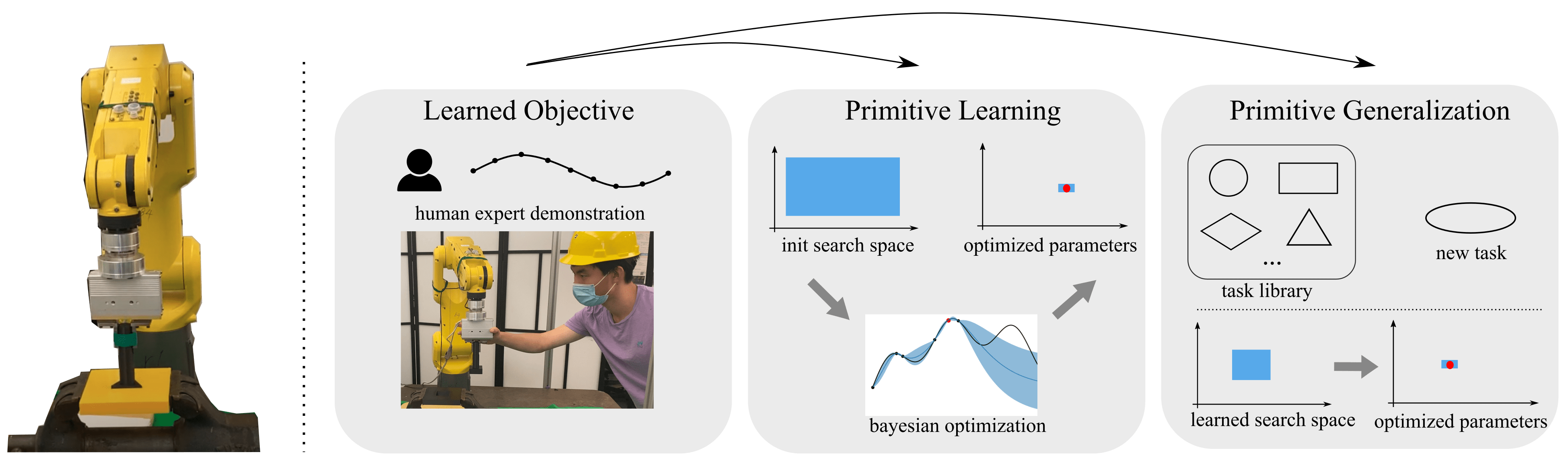
Figure 1: An overview of Prim-LAfD. Prim-LAfD learns a dense objective function from human demonstrations. It applies Bayesian Optimization (BO) to learn the primitive parameters w.r.t. the learned objective function. When generalizing to unseen tasks, we first select similar tasks from the task library based on the introduced similarity metric and then obtain a transferable search space for the new task for BO.

2 Related Work

Robotic assembly tasks, e.g., peg insertion, have been studied for decades and are still one of the most popular and challenging topics in the robotics community Lian et al. (2021). Recently, many works have focused on developing learning algorithms for assembly tasks, among which deep reinforcement learning (RL) methods gained the most attention. For example, Lee et al. (2019) proposes a self-supervised learning method to learn a neural representation from sensory input and used the learned representation as the input of deep RL. In Wu et al. (2021), a reward learning approach is proposed to learn rewards from the high dimensional sensor input, and the reward is used to train a model-free RL policy. Nevertheless, these methods suffer from data inefficiency when facing novel tasks. There are also some works that combine RL and learning from demonstrations (LfD) to address the above issue Vecerik et al. (2017); Davchev et al. (2022). However, the impractical amount of robot-environment interactions required by deep RL algorithms and the domain expertise needed to adapt to different insertion tasks limit their adoption in real-world, particularly industrial scenarios.

By contrast, motion primitives, implemented with hybrid motion/force or impedance controllers, are often used for insertion tasks in practice. Johannsmeier et al. (2019) makes the first attempt to learn the primitive parameters via black-box optimizers, minimizing the task completion time. This algorithm work effectively if primitive parameter ranges are narrowly set; otherwise, due to the sparse reward choice, it takes a large amount of robot-environment interactions for the optimizer to escape the parameter region leading to unsuccessful executions. In comparison, we propose a model-based dense objective function learned from demonstration, which guides the optimizer to explore more promising parameter regions earlier in training.

Transferring the existing policies to novel tasks is extensively studied in the field of robotic manipulation recently. It is especially important for RL based approaches, as most RL algorithms consider to learn a task in simulation first and then transfer the policy to the real world. One common approach is domain randomization, in which a variety of tasks are trained in simulation in order to capture the task distribution Tobin et al. (2017); Peng et al. (2018). Meta-RL has gained significant attraction in recent years Rakelly et al. (2019), where the experience within a family of tasks can be adapted to a new task in that family. However, for motion primitive learning methods, often optimized with gradient-free parameter search methods Johannsmeier et al. (2019); Voigt et al. (2020), there haven’t been efforts to transfer such prior experience to similar tasks. To the best of our knowledge, our work is the first attempt to encode the prior experiences and reduce the parameter exploration space during primitive learning on a novel insertion task.

3 Proposed Method

In this section, we provide more details of Prim-LAfD for insertion tasks.

3.1 Cartesian Impedance Control and the State-Action Space

Impedance control is used to render the robot as a mass-spring-damping system following the dynamics below,

$$\mathbf{M}(\mathbf{\ddot{x}}-\mathbf{\ddot{x}}_{d})+\mathbf{D}(\mathbf{\dot{x}}-\mathbf{\dot{x}}_{d})+\mathbf{K}(\mathbf{x}-\mathbf{x_{d}})=-\mathbf{F}_{ext},$$ (1)

where $\mathbf{M}$, $\mathbf{D}$, $\mathbf{K}$ are the desired mass, damping, and stiffness matrices, and $\mathbf{F}_{ext}$ denotes the external wrench. $\mathbf{\ddot{x}}_{d}$, $\mathbf{\dot{x}}_{d}$, $\mathbf{x}_{d}$ are the desired Cartesian acceleration, velocity, and pose of the end-effector, and $\mathbf{\ddot{x}}$, $\mathbf{\dot{x}}$, $\mathbf{x}$ are the current values correspondingly. We assume a small velocity in our tasks and set $\mathbf{\ddot{x}}$, $\mathbf{\dot{x}}$ to 0, thus arriving at this control law,

$$\begin{split}\boldsymbol{\tau}&=\mathbf{J}(\mathbf{q})^{T}\mathbf{F},\\ \mathbf{F}&=-\mathbf{K}(\mathbf{x}-\mathbf{x_{d}})-\mathbf{D}\mathbf{\dot{x}}+\mathbf{g}(\mathbf{q}),\end{split}$$ (2)

where $\boldsymbol{\tau}$ is the control torque, $\mathbf{F}$ is the control wrench, $\mathbf{J}(\mathbf{q})$ is the Jacobian, and $\mathbf{g}(\mathbf{q})$ is the gravity compensation force.

Throughout an insertion task, we would like to design a desired trajectory and a variable impedance to guide the robot movement. In favor of stability and ease of learning, we use a diagonal stiffness matrix $\mathbf{K}=\textbf{Diag}[K_{x},K_{y},K_{z},K_{roll},K_{pitch},K_{yaw}]$, and, for simplicity, the damping matrix $\mathbf{D}$ is scaled such that the system is critically damped.

In summary, our insertion policy output, $\mathbf{a}_{t}\in\mathcal{A}$, fed to the impedance controller defined above, is composed of a desired end-effector pose $\mathbf{x}_{d}$ and the diagonal elements of the stiffness matrix $\mathbf{k}=\{K_{x},K_{y},K_{z},K_{roll},K_{pitch},K_{yaw}\}$. The input to the policy, $\mathbf{s}_{t}\in\mathcal{S}$, consists of end-effector pose $\mathbf{x}_{t}$ and the sensed wrench $\mathbf{f}_{t}$, and is extensible to more modalities such as RGB and depth images.

3.2 Manipulation Policy with Motion Primitives

In this section, we provide a detailed design on our insertion policy, which entails a state machine with state-dependent motion primitives. Each motion primitive $\mathcal{P}_{m}$ associated with the $m$-th state defines a desired trajectory $f_{\boldsymbol{\theta}_{m}}(\mathbf{x}_{enter},\mathcal{T})$, an exit condition checker $h_{\boldsymbol{\theta}_{m}}(\cdot):\mathcal{S}\rightarrow\{1,0\}$, and a 6-dimensional stiffness vector $\mathbf{k}_{m}$. $\boldsymbol{\theta}_{m}$ contains all the learnable parameters in the primitive $\mathcal{P}_{m}$. $\mathbf{x}_{enter}$ denotes the end-effector pose upon entering the $m$-th state. $\mathcal{T}$ contains the task information such as the 6 DoF poses of the peg and the hole; often, the hole pose defines the task frame of the motion primitives.

In the following, we formally describe the $4$ motion primitives used in the peg-in-hole tasks, as shown in Figure 2.

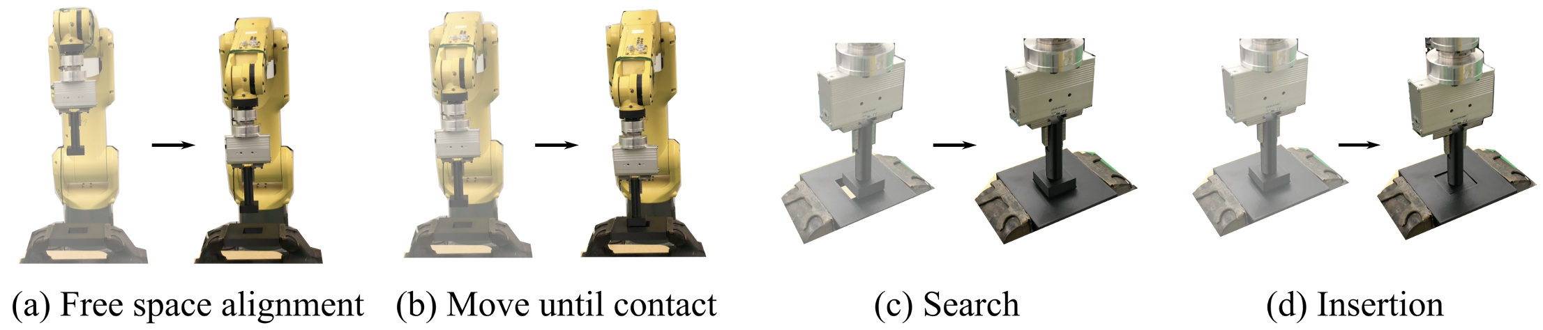
Figure 2: An illustrative figure of the motion primitives designed for peg-in-hole tasks. We show the start and the end states of the robot for each primitive.

Free space alignment.

The end-effector moves to an initial alignment pose.

$$\begin{split}f_{\boldsymbol{\theta}_{1}}&=u(\mathbf{x}_{enter},\mathbf{x}_{target})\\ \quad h_{\boldsymbol{\theta}_{1}}(\mathbf{s}_{t})&=\mathbb{I}\left[||\mathbf{x}_{t}-\mathbf{x}_{target}||_{2}<\sigma\right]\\ \quad\mathbf{k}_{1}&=\mathbf{k}_{max}.\end{split}$$ (3)

where $\mathbb{I}[\cdot]$ is an indicator function mapping the evaluated condition to $\{0,1\}$. $u(\cdot,\cdot)$ generates a linearly interpolated motion profile from the first to the second pose provided. The target end-effector pose $\mathbf{x}_{target}$ is extracted from the task information $\mathcal{T}$ as $\mathbf{x}_{target}=T_{hole}^{base}\cdot T^{hole}_{peg}\cdot T^{peg}_{ee}$, where $T_{hole}^{base}$ and $T^{peg}_{ee}$ denote the detected hole pose in robot base frame and the end-effector pose in peg frame. $T^{hole}_{peg}$ is the desired peg pose in hole frame when the peg is above and coarsely aligned with the hole. $\mathbf{k}_{max}$ denotes a 6-dimensional vector composed of the highest stiffness values along each axis. $\sigma$ is a pre-defined threshold to determine if the robot arrives at the desired pose. No learnable parameters exist in this primtive. The parameters in this $1$-st primitive involves $\boldsymbol{\theta}_{1}=\{\O\}$.

Move until contact.

The end-effector moves towards the hole until the peg is in contact with the hole top surface.

$$\begin{split}f_{\boldsymbol{\theta}_{2}}&=u(\mathbf{x}_{enter},\mathbf{x}_{enter}-\left[0\;0\;\delta\;0\;0\;0\right]^{T})\\ h_{\boldsymbol{\theta}_{2}}(\mathbf{s}_{t})&=\mathbb{I}[f_{t,z}>\eta]\\ \mathbf{k}_{2}&=\mathbf{k}_{max}.\end{split}$$ (4)

$\delta$ is the desired displacement along z-axis in the task frame, $f_{t,z}$ is the sensed force along z-axis at time $t$, and $\eta$ is the exit force threshold. Therefore the parameters defining this $2$-nd primitive consists of $\boldsymbol{\theta}_{2}=\{\delta,\eta\}$.

Search.

The robot searches for the location of the hole while keeping in contact with the hole until the peg and the hole are perfectly aligned. After empirical comparisons with alternatives, including the commonly used spiral search, we choose the Lissajous curve as the searching pattern, which gives the most reliable performance. While searching for the translation alignment, the peg simultaneously rotates along the z-axis to address the yaw orientation error. The roll and pitch orientation errors are expected to be corrected by the robot being compliant to the environment with the learned stiffness.

$$\begin{split}f_{\boldsymbol{\theta}_{3}}(t)&=\mathbf{x}_{enter}+\left[\begin{matrix}Asin(2\pi a\frac{n_{1}}{T}t)\\ Bsin(2\pi b\frac{n_{1}}{T}t)\\ -\gamma\\ 0\\ 0\\ \varphi sin(2\pi\frac{n_{2}}{T}t)\end{matrix}\right]\\ h_{\boldsymbol{\theta}_{3}}(\mathbf{s}_{t})&=\mathbb{I}[{x}_{enter,z}-{x}_{t,z}>\zeta]\\ \mathbf{k}_{3}&=\mathbf{k}_{search},\end{split}$$ (5)

where $a=7,b=6$ are the Lissajous numbers selected and $T$ is the cycle period in Lissajous search, $\varphi$ is the maximum tolerated yaw error of the estimated hole pose, set as 6 degree in our experiments. The learnable parameters of this primitive are $\boldsymbol{\theta}_{3}=\{A,B,\frac{n_{1}}{T},\frac{n_{2}}{T},\gamma,\zeta,\mathbf{k}_{search}\}$.

Insertion.

The peg is inserted into the hole in a compliant manner.

$$\begin{split}f_{\boldsymbol{\theta}_{4}}&=u(\mathbf{x}_{enter},\mathbf{x}_{enter}-\left[0\;0\;\lambda\;0\;0\;0\right]^{T})\\ h_{\boldsymbol{\theta}_{3}}&=\mathbb{I}[\textrm{success condition}]\\ \mathbf{k}_{4}&=\mathbf{k}_{insertion},\end{split}$$ (6)

where the success condition is provided by the task information $\mathcal{T}$, e.g., $||\mathbf{x}_{t}-\mathbf{x}_{success}||_{2}<\epsilon$. The primitive parameters to learn are $\boldsymbol{\theta}_{4}=\{\lambda,\mathbf{k}_{insertion}\}$.

3.3 Learning Primitive Parameters

In this section, we illustrate how to learn the primitive parameters $\boldsymbol{\Theta}=\{\boldsymbol{\theta}_{1},\boldsymbol{\theta}_{2},\boldsymbol{\theta}_{3},\boldsymbol{\theta}_{4}\}$. The core idea is using a black-box optimizer to optimize a task-relevant objective function $J(\cdot)$. While a similar idea has been explored in Johannsmeier et al. (2019), the objective function used is simply the measured task execution time. The major drawback of this objective function is that the objective signal is sparse and can only be triggered when the task is successfully executed. This makes the optimizer challenging to find a feasible region initially, especially when the primitive parameter space is large. Motivated by this, we propose a dense objective function that measures the likelihood of the induced execution trajectory being sampled from the distribution of successful task demonstrations $\mathcal{E}_{D}=\{\boldsymbol{\xi_{i}}\}(i=1,2,...,M)$. Assuming the trajectroies are Markovian, a trajectory rollout $\boldsymbol{\xi}=[\boldsymbol{x}_{0},\boldsymbol{x}_{1},...,\boldsymbol{x}_{n-1}]$ is modeled as:

$$p(\boldsymbol{\xi};\boldsymbol{\Theta})=p(\boldsymbol{x}_{0})\prod_{i=1}^{n-1}p(\boldsymbol{x}_{i}|\boldsymbol{x}_{i-1}).$$ (7)

In order to learn $p(\boldsymbol{x}_{i}|\boldsymbol{x}_{i-1})$ from demonstrations, we first use a Guassian Mixture Model (GMM) to model the joint probability as $p(\left[\begin{matrix}\boldsymbol{x}_{i}\\ \boldsymbol{x}_{i-1}\end{matrix}\right])=\sum_{j=1}^{K}{\phi_{j}\mathcal{N}(\boldsymbol{\mu}_{j},\boldsymbol{\Sigma}_{j})}$ , where $\sum_{j=1}^{K}{\phi_{j}}=1$, and $K$ is the number of GMM clusters.

We further represent the Gaussian mean $\boldsymbol{\mu}_{j}$ and variance $\boldsymbol{\Sigma}_{j}$ as: $\boldsymbol{\mu}_{{j}}=\begin{bmatrix}\boldsymbol{\mu}^{{1}}_{{j}}\\ \boldsymbol{\mu}^{{2}}_{{j}}\end{bmatrix}$, $\boldsymbol{\Sigma}_{{j}}=\begin{bmatrix}\boldsymbol{\Sigma}^{{11}}_{{j}}&\boldsymbol{\Sigma}^{{12}}_{{j}}\\ \boldsymbol{\Sigma}^{{21}}_{{j}}&\boldsymbol{\Sigma}^{{22}}_{{j}}\end{bmatrix}$. We can then derive the conditional probability $p(\boldsymbol{x}_{i}|\boldsymbol{x}_{i-1})=\sum_{j=1}^{K}{\phi_{j}\mathcal{N}(\overline{\boldsymbol{\mu}}_{j},\overline{\boldsymbol{\Sigma}}_{j})}$, where

$$\begin{split}\overline{\boldsymbol{\mu}}_{j}&=\boldsymbol{\mu}^{1}_{j}+\boldsymbol{\Sigma}^{12}_{j}(\boldsymbol{\Sigma}^{22}_{j})^{-1}(\boldsymbol{x}_{i-1}-\boldsymbol{\mu}^{2}_{j})\\ \overline{\boldsymbol{\Sigma}}_{j}&=\boldsymbol{\Sigma}^{11}_{j}-\boldsymbol{\Sigma}^{12}_{j}(\boldsymbol{\Sigma}^{22}_{j})^{-1}\boldsymbol{\Sigma}^{21}_{j}.\end{split}$$ (8)

Then, the objective function is designed as $J(\boldsymbol{\xi})=\log{p(\boldsymbol{\xi};\boldsymbol{\Theta})}+B$, where the first term encourages exploring parameters inducing similar trajectories to the successful demonstration traces, and the second term $B$ denotes a sparse bonus reward if the task succeeds. We use black-box optimizers to solve $\boldsymbol{\Theta}^{*}=\underset{\boldsymbol{\Theta}}{\mathrm{argmax}}J(\boldsymbol{\Theta})$, and Bayesian Optimization (BO) is selected in our work. Expected Improvement (EI) is used as the acquisition function, and we run BO for $N$ iterations. The learned parameter $\boldsymbol{\Theta}^{*}$ that achieves maximum $J(\boldsymbol{\Theta})$ during $N$ training iterations is selected as the optimal primitive configuration. Note that BO can be seamlessly replaced by other black-box optimization methods and the optimizer choice is not the focus of this work.

3.4 Task Generalization

In this section, we detail our method on how to leverage prior experience when adapting to a novel insertion task, in particular, how to adapt previously learned peg-in-hole policies to different tasks with unseen hole shapes. Our adaptation procedure is composed of two core steps: measuring task similarities and transferring similar task policies to the unseen shape.

3.4.1 Measuring task similarity

Given an insertion skill library, i.e., a set of learned peg insertion policies for different shapes, $\mathcal{M}=\{\pi_{1}({\boldsymbol{\Theta}_{1}}),\pi_{2}({\boldsymbol{\Theta}_{2}}),...,\pi_{n}({\boldsymbol{\Theta}_{n}})\}$ and an unseen shape, our goal is to first identify which subset of the $n$ tasks are most relevant to the new task. While there is a diverse range of auxiliary task information that can be used to measure task similarity, here, we define the task similarity as the similarity between the hole cross-section contours. This assumption is based on the intuition that similar hole shapes would induce similar policies for insertion. For example, the insertion policies for a square hole and a rectangle hole are likely to be similar, and the optimal policy for a round hole might still work for a hexadecagon hole. The similarity between a shape pair is measured by the $L_{1}$ distance between the two shapes’ turning functions Arkin et al. (1991).

Turning functions are a commonly used representation in shape matching, which represents the angle between the counter-clockwise tangent and the x-axis as a function of the travel distance along a normalized polygonal contour. After obtaining the shape distances of the unseen shape and each shape in the task library, we choose the top $L$ shapes that are closest to the unseen shape as similar shapes. The policies of the similar shapes are then used as input for transfer learning detailed below in Section 3.4.2.

3.4.2 Adapting to unseen shapes

Given a novel task, our goal is to efficiently adapt the already learned insertion policies of the most similar shapes. We build upon BO with hyperparameter transfer Perrone et al. (2019). Unlike many works framing BO transfer learning as a multi-task learning problem, we attempt to learn the search space of BO from similar task policies and apply it to learning for the new task.

Specifically, let $\mathcal{T}=\{T_{1},T_{2},...,T_{t}\}$ denote the task set of different hole shapes we selected as described in Section 3.4.1, and $\mathcal{F}=\{J_{1},J_{2},...,J_{t}\}$ denotes the corresponding objective functions for each task. All the objective functions are initially defined on a common search space $\mathcal{X}\subseteq\mathrm{R}^{|\boldsymbol{\Theta}|}$, and it’s assumed that we already obtained the optimal policies for the $t$ tasks $\{\pi_{1}(\boldsymbol{\Theta}_{1}^{\star}),\pi_{2}(\boldsymbol{\Theta}_{2}^{\star}),...,\pi_{t}(\boldsymbol{\Theta}_{t}^{\star})\}(\boldsymbol{\Theta}_{i}^{\star}\in\mathcal{X})$. Given an unseen task $T_{t+1}$, we aim to learn a new search space $\overline{\mathcal{X}}\subseteq\mathcal{X}$ from the previous tasks to expedite the new task learning process. We define the new search space as $\overline{\mathcal{X}}=\{\boldsymbol{\Theta}\in\mathrm{R}^{|\boldsymbol{\Theta}|}|\mathbf{l}\leq\boldsymbol{\Theta}\leq\mathbf{u}\}$, where $\mathbf{l},\mathbf{u}$ are the lower and upper bounds. It was proved in Perrone et al. (2019) that the new search space can be obtained by solving the constrained optimization problem:

$$\min_{\mathbf{l},\mathbf{u}}{\frac{1}{2}||\mathbf{u}-\mathbf{l}||_{2}^{2}}\textrm{ such that for }1\leq i\leq t,\mathbf{l}\leq\boldsymbol{\Theta}_{i}^{\star}\leq\mathbf{u}.$$ (9)

The optimization problem has a closed-form solution:

$$\mathbf{l}^{\star}=\min\{\boldsymbol{\Theta}_{i}^{\star}\}_{i=1}^{t},\mathbf{u}^{\star}=\max\{\boldsymbol{\Theta}_{i}^{\star}\}_{i=1}^{t}.$$ (10)

This new search space is then utilized for policy training of this unseen shape task, following the procedure described in Section 3.3.

4 Experimental Results

We aim to investigate the effectiveness of Prim-LAfD by answering two questions: 1) whether the dense objective function proposed in Section 3.3 expedites the primitive learning process and improves policy performance, and 2) whether the generalization algorithm described in Section 3.4 is effective when transferring to an unseen shape. An insertion task library of 8 different peg-hole pairs is constructed, including 6 representative 3D-printed geometry shapes (round, triangle, parallelogram, rectangle, hexadecagon, ellipse) and two common industrial connectors (RJ45, waterproof). Examples are shown in Figure 3.

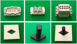
Figure 3: Two peg-hole pair instances (waterproof and parallelogram) used in our experiments.

4.1 Experimental Setup

As shown in Figure 1, our hardware setup consists of a 6-DoF FANUC Mate 200iD robot and an ATI Mini45 Force/Torque sensor. The clearances for all 3D printed peg-hole pairs are 1mm; the waterproof and RJ45 are unaltered off-the-shelf connectors. To mimic the pose estimation error during industrial deployments, a uniform perturbation error of +/- 5mm in translation and +/- 6 degree in orientation is applied along each dimension. The controller takes the policy output at 10 Hz and computes the torque command streamed to the robot at 1000Hz. All the learnable parameters of the policy and their initial range are listed in Table 1. Two metrics are used to evaluate the effectiveness and efficiency of the approaches: 1) the number of iterations the robot takes to accomplish the first successful insertion during training (denoted as number of iterations), and 2) the success rate of the optimal policy after a fixed number of iterations (denoted as success rate).

Table 1: Learnable parameters and corresponding range in the motion primitives.

	Move until contact		Search							Insertion
Parameters	$\delta{(m)}$	$\eta{(N)}$	$A{(m)}$	$B{(m)}$	$n_{1}/T{(s^{-1})}$	$n_{2}/T{(s^{-1})}$	$\gamma{(m)}$	$\zeta{(m)}$	$\mathbf{k}_{search}{(N/m,Nm/rad)}$	$\lambda{(m)}$	$\mathbf{k}_{insertion}{(N/m,Nm/rad)}$
min	$0$	$1$	$0$	$0$	$0/60$	$0/60$	$0$	$0$	$\mathbf{0}^{[6\times 1]}$	$0$	$\mathbf{0}^{[6\times 1]}$
max	$0.1$	$10$	$0.02$	$0.02$	$2/10$	$20/10$	$0.02$	$0.02$	$[\mathbf{600}^{[3\times 1]},\mathbf{40}^{3\times 1}]$	$0.05$	$[\mathbf{600}^{[3\times 1]},\mathbf{40}^{3\times 1}]$

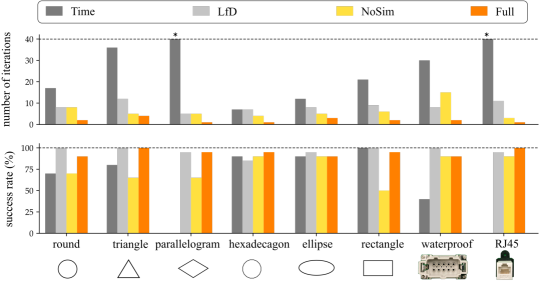
Figure 4: Experimental results for primitive learning and generalization. Time: primitive learning using task execution time as objective function, LfD: primitive learning using learned objective function (Section 3.3), NoSim: primitive generalization without measuring task similarities, Full: full generalization method (Section 3.4). $\star$ represents no successful trials is found during the learning process.

4.2 Learning Primitive Parameters

In this experiment, we applied our learned objective function from demonstration (LfD) for primitive parameter optimization as described in Section 3.3, and compare the results against primitive optimization by minimizing the measured task execution time (Time) Johannsmeier et al. (2019). When learning the objective function, we collected $10$ demonstrations for each insertion task through kinesthetic teaching. The demonstrations have $43.5$ time steps on average across different insertion tasks. The number of GMM clusters is set as $K=25$.

For each of the 8 peg-hole pairs, we run BO for 40 iterations. Within each iteration, the current policy is executed twice with independently sampled hole poses. The average objective of the two trials is used as the final objective value consumed by the BO step. The optimal policy is selected as the policy at the BO step achieving the optimal objective value, and evaluated by being executed 20 trials with independently sampled hole poses. As shown in Figure 4, LfD outperforms Time on almost all the insertion tasks in both number of iterations and success rate. In some tasks, e.g., parallelogram and RJ45, Time cannot find proper parameters to achieve a single successful trial within 40 iterations, while LfD successfully navigates through the parameter space and accomplishes successful trials for all of the tasks. This validates the learned dense objective function, provides richer information for primitive learning than sparse signals alone like task success and completion time.

4.3 Generalizing to Unseen Shapes

We now examine how our generalization method described in Section 3.4 performs when transferring to unseen shapes. We consider the leave-one-out cross-validation setting, i.e., when presented 1 of the 8 tasks as the task of interest, the learning algorithm has access to all interaction data during policy learning on the other 7 tasks. Two sets of experiments are conducted. First, we apply the full method described in Section 3.4 (Full) to learn a reduced search space using the $L=3$ most similar tasks, within which the primitive parameters are optimized.

Compared with LfD where parameters are optimized over the full space, Full reached a comparable or better success rate, meanwhile achieved the first task completion with a lower number of iterations. Second, we consider learning the search space without measuring the task similarities (NoSim), i.e., the new search space is obtained using all the other tasks instead of only the similar ones. As seen in Figure 4, Full outperforms NoSim consistently on all insertion tasks, indicating the significance of finding similar tasks using the task geometry information before learning the new search space.

5 Conclusion

We propose Prim-LAfD, a data-efficient framework for learning and generalizing insertion skills with motion primitives. Extensive experiments on 8 different peg-hole and connector-socket insertion tasks are conducted to demonstrate the advantages of our method. The results show that Prim-LAfD enables a physical robot to learn peg-in-hole manipulation skills and to adapt the learned skills to unseen tasks at low time cost.

References

- Alt et al. (2021) Alt, B., Katic, D., Jäkel, R., Bozcuoglu, A.K., and Beetz, M. (2021). Robot program parameter inference via differentiable shadow program inversion. In International Conference on Robotics and Automation (ICRA), 4672–4678. IEEE.
- Arkin et al. (1991) Arkin, E.M., Chew, L.P., Huttenlocher, D.P., Kedem, K., and Mitchell, J.S. (1991). An efficiently computable metric for comparing polygonal shapes. Technical report, CORNELL UNIV ITHACA NY.
- Davchev et al. (2022) Davchev, T., Luck, K.S., Burke, M., Meier, F., Schaal, S., and Ramamoorthy, S. (2022). Residual learning from demonstration: Adapting dmps for contact-rich manipulation. IEEE Robotics and Automation Letters, 7(2), 4488–4495.
- Gu et al. (2017) Gu, S., Holly, E., Lillicrap, T., and Levine, S. (2017). Deep reinforcement learning for robotic manipulation with asynchronous off-policy updates. In international conference on robotics and automation (ICRA), 3389–3396. IEEE.
- Johannsmeier et al. (2019) Johannsmeier, L., Gerchow, M., and Haddadin, S. (2019). A framework for robot manipulation: Skill formalism, meta learning and adaptive control. In International Conference on Robotics and Automation (ICRA), 5844–5850. IEEE.
- Kalashnikov et al. (2018) Kalashnikov, D., Irpan, A., Pastor, P., Ibarz, J., Herzog, A., Jang, E., Quillen, D., Holly, E., Kalakrishnan, M., Vanhoucke, V., et al. (2018). Scalable deep reinforcement learning for vision-based robotic manipulation. In Conference on Robot Learning, 651–673. PMLR.
- Lee et al. (2019) Lee, M.A., Zhu, Y., Srinivasan, K., Shah, P., Savarese, S., Fei-Fei, L., Garg, A., and Bohg, J. (2019). Making sense of vision and touch: Self-supervised learning of multimodal representations for contact-rich tasks. In International Conference on Robotics and Automation (ICRA), 8943–8950. IEEE.
- Li et al. (2020) Li, T., Srinivasan, K., Meng, M.Q.H., Yuan, W., and Bohg, J. (2020). Learning hierarchical control for robust in-hand manipulation. In International Conference on Robotics and Automation (ICRA), 8855–8862. IEEE.
- Lian et al. (2021) Lian, W., Kelch, T., Holz, D., Norton, A., and Schaal, S. (2021). Benchmarking off-the-shelf solutions to robotic assembly tasks. In International Conference on Intelligent Robots and Systems (IROS), 1046–1053. IEEE.
- Peng et al. (2018) Peng, X.B., Andrychowicz, M., Zaremba, W., and Abbeel, P. (2018). Sim-to-real transfer of robotic control with dynamics randomization. In international conference on robotics and automation (ICRA), 3803–3810. IEEE.
- Perrone et al. (2019) Perrone, V., Shen, H., Seeger, M.W., Archambeau, C., and Jenatton, R. (2019). Learning search spaces for bayesian optimization: Another view of hyperparameter transfer learning. Advances in Neural Information Processing Systems, 32.
- Rakelly et al. (2019) Rakelly, K., Zhou, A., Finn, C., Levine, S., and Quillen, D. (2019). Efficient off-policy meta-reinforcement learning via probabilistic context variables. In International conference on machine learning, 5331–5340. PMLR.
- Tobin et al. (2017) Tobin, J., Fong, R., Ray, A., Schneider, J., Zaremba, W., and Abbeel, P. (2017). Domain randomization for transferring deep neural networks from simulation to the real world. In international conference on intelligent robots and systems (IROS), 23–30. IEEE.
- Vecerik et al. (2017) Vecerik, M., Hester, T., Scholz, J., Wang, F., Pietquin, O., Piot, B., Heess, N., Rothörl, T., Lampe, T., and Riedmiller, M. (2017). Leveraging demonstrations for deep reinforcement learning on robotics problems with sparse rewards. arXiv preprint arXiv:1707.08817.
- Voigt et al. (2020) Voigt, F., Johannsmeier, L., and Haddadin, S. (2020). Multi-level structure vs. end-to-end-learning in high-performance tactile robotic manipulation.
- Vuong et al. (2021) Vuong, N., Pham, H., and Pham, Q.C. (2021). Learning sequences of manipulation primitives for robotic assembly. In International Conference on Robotics and Automation (ICRA), 4086–4092. IEEE.
- Wu et al. (2021) Wu, Z., Lian, W., Unhelkar, V., Tomizuka, M., and Schaal, S. (2021). Learning dense rewards for contact-rich manipulation tasks. In International Conference on Robotics and Automation (ICRA), 6214–6221. IEEE.