StructVPR: Distill Structural Knowledge with Weighting Samples
for Visual Place Recognition

Abstract

Visual place recognition (VPR) is usually considered as a specific image retrieval problem. Limited by existing training frameworks, most deep learning-based works cannot extract sufficiently stable global features from RGB images and rely on a time-consuming re-ranking step to exploit spatial structural information for better performance. In this paper, we propose StructVPR, a novel training architecture for VPR, to enhance structural knowledge in RGB global features and thus improve feature stability in a constantly changing environment. Specifically, StructVPR uses segmentation images as a more definitive source of structural knowledge input into a CNN network and applies knowledge distillation to avoid online segmentation and inference of seg-branch in testing. Considering that not all samples contain high-quality and helpful knowledge, and some even hurt the performance of distillation, we partition samples and weigh each sample’s distillation loss to enhance the expected knowledge precisely. Finally, StructVPR achieves impressive performance on several benchmarks using only global retrieval and even outperforms many two-stage approaches by a large margin. After adding additional re-ranking, ours achieves state-of-the-art performance while maintaining a low computational cost.

1 Introduction

Visual place recognition (VPR) is a critical task in autonomous driving and robotics, and researchers usually regard it as an image retrieval problem[28, 54, 30]. Given a query RGB image from a robot, VPR aims to determine whether the robot has been to this place before and to identify the corresponding images from a database. Extreme environmental variations are challenging to methods, especially long-term changes (seasons, illumination, vegetation) and dynamic occlusions. Therefore, learning discriminative and robust features is essential to distinguish places.

There has been a commonly used two-stage strategy that retrieves candidates with global features and then re-ranks them through local descriptor matching, where re-ranking is time- and resource-consuming but dramatically improves the recall performance. The improvement is because geometric verification based on local features provides rich and explicit structural information, which has stronger robustness to VPR than appearance information in some aspects, such as shape, edge[3], spatial layout, and category[13]. Considering that segmentation (SEG) images have rich structural information, we tried some empirical studies using RGB and SEG as network input for VPR. We find that these two modalities have their advantages and disadvantages at the sample level, which means that better performance can be achieved if both modalities are appropriately fused. As Figure 1 shows, both modalities have specific cases they are better at recognizing.

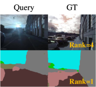
(a)

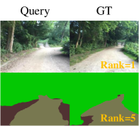
(b)

Figure 1: Examples of query images and ground truths. The marked number represents the recall performance of two pre-trained branches on ground truths. (a) shows the scene with illumination variation and seasonal changes, where segmentation images are more recognizable. (b) shows the scene with changing perspectives, where RGB images are more recognizable.

Based on the above discussion, we attempt to use the SEG modality to enhance structural knowledge in global RGB feature representation, achieving comparable performance to re-ranking while maintaining low computational cost. Complementarity of the two modalities on samples, that is, some samples may contain harmful knowledge for RGB, inspires us to perform knowledge enhancement selectively. Therefore, we propose a new knowledge distillation (KD) architecture, StructVPR, which can effectively distill the high-quality structural representations from the SEG modality to the RGB modality. Specifically, StructVPR uses RGB images and encoded segmentation label maps for separate pre-training with VPR loss, uses two pre-trained branches to partition samples, and then weights the distillation loss to selectively distill the high-quality knowledge of the pre-trained seg-branch into the final RGB network. Note that the concept of “sample” is a sample pair with a query and a labeled positive. Compared with non-selective distillation methods[9] and previous selective distillation works[50], StructVPR can exactly mine those suitable samples on which the teacher network performs good and better than the student and distinguish the importance of sample knowledge for KD. Moreover, overly refined segmentation is not helpful, and the importance of all semantic classes varies for VPR. Hence, we cluster original classes according to the sensitivity to objects in VPR and introduce prior information of labels via weighted one-hot encoding.

Our main contributions can be highlighted as follows: 1) The overall architecture avoids the computation and inference of segmentation during testing by distilling the high-quality knowledge from the SEG modality to the RGB modality, where segmentation images are pre-encoded into weighted one-hot label maps to extract structural information for VPR. 2) To the best of our knowledge, there is no previous work in VPR concerning selecting suitable samples for distillation. StructVPR forges a connection between sample partition with student network participating and weighted knowledge distillation for each sample. 3) We perform comprehensive experiments on key benchmarks. StructVPR performs better than global methods and achieves comparable performance to many two-stage (global-local) methods. The consistent improvement in all datasets corroborates the effectiveness and robustness of StructVPR. Experimental results show that StructVPR achieves SOTA performance with low computational cost compared with global methods, and it is also competitive with most two-stage approaches [6, 20]. StructVPR with re-ranking outperforms the SOTA VPR approaches (4.475$\%$ absolute increase on Recall$@5$ compared with the best baseline[51]).

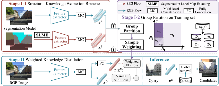
Figure 2: Illustration of the proposed pipeline. We first pre-train two branches with VPR supervision to extract structural knowledge, and then we perform offline group partition and weighting on samples. Then weighted knowledge distillation and VPR supervision are performed in Stage II. During testing, StructVPR avoids the computation and inference of segmentation, using only the trained model in Stage II. More importantly, it can maximize the efficiency of distilling high-quality knowledge.

2 Related Work

Visual Place Recognition. Most of the research on VPR has focused on constructing better image representations to perform retrieval. The common way to represent a single RGB image is to use global descriptors or local descriptors. More recently, using CNNs to build local descriptors has achieved superior performances[32, 11, 24, 5]. Global descriptors can be generated by directly extracting[58, 8, 16, 38, 40] or aggregating local descriptors. For aggregation, traditional methods have been incorporated into CNN-based architectures [1, 31]. To achieve a good compromise between accuracy and efficiency, a widely used architecture is to rank the database by global features, and then re-rank the top candidates[29, 43]. Many studies have verified its validity [42, 45, 48, 46].

Recently, many methods [36, 37, 35, 56, 57] try to introduce semantics into RGB features by using attention mechanism or additional information. TransVPR[51] introduces the attention mechanism to guide models to focus on invariant regions and extract robust representations. DASGIL[23] uses multi-task architecture with a single shared encoder to create global representation, and uses domain adaptation to align models on synthetic and real-world datasets. Based on [23], [34] focuses on filtering semantic information via an attention mechanism.

Knowledge Distillation. It is an effective way to enrich models with knowledge distillation (KD)[17]. It extracts specific knowledge from a stronger model (i.e., “teacher”) and transfer to a weaker model (i.e., “student”) through additional training signals. There has been a large body of work on transferring knowledge with the same modality, such as model compression[4, 7, 21] and domain adaptation[26, 2]. However, the data or labels for some modalities might not be available during training or testing, so it is essential to distill knowledge between different modalities [39, 55]. [12, 22] generate a hallucination network to model depth information and enforce it for RGB descriptors learning. In this way, the student learns to simulate a virtual depth that improves the inference performance. In this work, we construct a weighted knowledge distillation architecture to distill and enhance high-quality structural knowledge into RGB features.

Nevertheless, these previous works enhance the target model by transferring knowledge on each training sample from the teacher model, rarely discussing the difference about knowledge among samples [27, 14]. Wang et al. [50] proposes to select suitable samples for distillation through analyzing the teacher network. Differently, our solution considers both pre-trained teacher and student network in sample partition and weight the distillation loss for samples.

3 Methodology

Considering that re-ranking with local features can provide rich and explicit structural knowledge, we try to utilize segmentation images to embed rich structural knowledge into RGB global retrieval and achieve comparable performance to two-stage methods. The key idea of StructVPR is very general: selectively distill high-quality and helpful knowledge into a single-input model by weighting samples. StructVPR includes two training stages: structural knowledge extraction and group partition, and weighted knowledge distillation. Figure 2 explains how StructVPR works.

3.1 Overview

Given an input RGB image $I^{R}$, its pairwise segmentation image $I^{S}$ is extracted by an open-source semantic segmentation model and converted into a fixed-size label map via segmentation label map encoding (SLME) module.

Then the seg-branch and rgb-branch are pre-trained with VPR loss. Based on the two pre-trained branches and designed evaluation rules, training sets can be partitioned, and different groups represent samples with different performances of seg-branch and rgb-branch. Given the domain knowledge in VPR, the concept of “sample” is generalized as a sample pair of a query and a positive. There are two specific aspects of domain knowledge: First, VPR datasets are often organized into query and database, in which each query image $q$ has a set of positive samples $\{p^{q}\}$ and a set of negative samples $\{n^{q}\}$. Second, the knowledge to be enhanced is feature invariance and robustness under changes between sample pairs in a scene.

Moreover, a weighting function is defined, and we perform weighted knowledge distillation and vanilla VPR supervision in Stage II.

3.2 Segmentation Label Map Encoding

It is nontrivial to convert segmentation images to a standard format before inputting them into the seg-branch, as each image contains a different number of semantic instances. As shown in Figure 2, the segmentation label map encoding (SLME) function encodes segmentation information to standard inputs of CNNs, including three steps: formatting, clustering, and weighting.

Firstly, like LabelEnc[19], we use a $C\times H\times W$ tensor to represent segmentation images, where $H\times W$ equals the RGB image size and $C$ is the number of semantic classes. Regions of the c-th class are filled with positive values in the c-th channel and 0 in other channels.

Secondly, derived from human experience, we incorporate the semantic labels that have similar effects on VPR, such as cars and bicycles being re-labeled as “dynamic objects”. It does this because too fine-grained segmentation will interfere with VPR like noises[34], which distracts model’s “attention” and increase the difficulty of model convergence, shown in Figure 3. Moreover, a large $C$ will lead to excessive computation. Moreover, this step lets models focus on useful parts and reduces computational costs.

Finally, based on the idea that each semantic class plays a different role in VPR task, we weigh positive values in the encoding as prior information to guide the optimization of models and accelerate their convergence. The attention mechanism of the human brain will allow humans to focus on iconic objects, such as buildings, while ignoring dynamic objects, such as pedestrians. In Section 4.4, experimental results corroborate our idea.

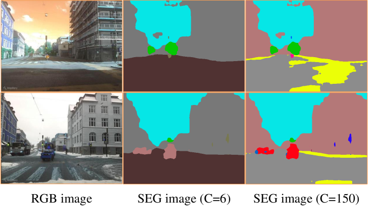
Figure 3: Visualization of clustered semantic classes. Shown from left to right are RGB images, 6-class segmentation images, and original segmentation images. It can be seen that the label space after clustering is cleaner for VPR.

3.3 Structural Knowledge Extraction

In the first training stage, we train seg-branch and rgb-branch to extract structural knowledge into features and prepare for subsequent group partition.

Rgb-branch. We use MobileNetV2[41] as our lightweight extractor. We remove the global average pooling layer and fully connected (FC) layer to obtain global features. According to the resolution of the feature maps, the backbone can be divided into 5 stages. The output feature maps are denoted as $\mathcal{F}^{R}_{1}$, $\mathcal{F}^{R}_{2},\mathcal{F}^{R}_{3},\mathcal{F}^{R}_{4},\mathcal{F}^{R}_{5}$, and the global feature is denoted as $\mathbf{x}^{R}$.

Seg-branch. Considering that segmentation label maps are more straightforward and have a higher semantic level than the paired RGB images, we adopt the depth stream in MobileSal[53] as the feature extractor in seg-branch. It has five stages with same strides and is not as large a capacity as MobileNetV2, denoted MobileNet-L in our paper. The output feature maps of five stages are denoted as $\mathcal{F}^{S}_{1},\mathcal{F}^{S}_{2},\mathcal{F}^{S}_{3},\mathcal{F}^{S}_{4},\mathcal{F}^{S}_{5}$, and the global feature is represented as $\mathbf{x}^{S}$.

Multi-level Concatenation (MC). In Figure 4, we first apply a global max pooling (GMP) layer to each feature map, $\mathcal{F}_{i}$, to compute single-level features, like

$$\mathbf{f}_{i} =\mathrm{L2Norm}(\mathrm{GMP}(\mathcal{F}_{i})),$$ (1)

and concatenate the features from the last 3 layers:

$$\mathbf{x} =\mathrm{L2Norm}(\mathrm{Concat}([\mathbf{f}_{3},\mathbf{f}_{4},\mathbf{f}_{5}])),$$ (2)

where $\mathbf{x}$ is the unified representation of global features.

Triplet VPR Loss. In two training stages, we adopt triplet margin loss[44] on $(q,p,n)$ as supervision:

$$\mathcal{L}_{vpr}(\mathbf{x})\!=\!\mathrm{max}(d(\mathbf{x}_{q},\mathbf{x}_{p})-d(\mathbf{x}_{q},\mathbf{x}_{n})+m,0),$$ (3)

where $\mathbf{x}_{q}$, $\mathbf{x}_{p}$, and $\mathbf{x}_{n}$ refer to global features of query, positive and negative samples. $d(\cdot)$ computes the $L2$ distance of two feature vectors, and margin $m$ is a constant parameter.

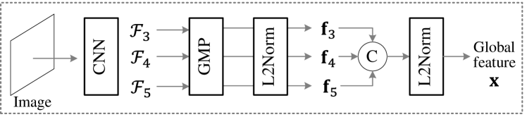
Figure 4: Visualization of Multi-level Concatenation.

3.4 Group Partition on Training Set

As mentioned above, not all samples contain high-quality and helpful teacher knowledge for the student, and even some will hurt the student’s performance. So what we need to do is to distill the expected knowledge precisely. This section addresses this problem simply yet effectively by selecting suitable samples.

Previous sample-based selective distillation works[50, 27, 14] rarely consider the student network with specific prior knowledge, resulting in a lack of teacher-student interaction in cross-modal cases. To avoid this, we let the two pre-trained branches in Section 3.3 participate in seeking a more accurate partition.

Partition Strategy. For convenience, “samples” mentioned below refer to sample pairs (see Section 3.1). In this section, we first did some preliminary empirical research, and we found that both pre-trained models have low VPR loss on training sets, but their Recall@$N$ performance cannot achieve 100$\%$ on training sets. Therefore, the performance of the two branches on a sample, $(q,p)$, can be compared as follows: the ranking of the positive $p$ in the recall list of the query $q$.

For convenience, recall rankings of samples of seg-branch and rgb-branch are denoted as $x$ and $y$, respectively. As shown in Figure 2, specific definitions for partitioning training sets are as follows:

$${\mathcal{D}_{1}} =\{(q,p)|x\leq{N_{t}},y>{N_{t}}\},$$

$${\mathcal{D}_{2}} =\{(q,p)|x\leq y\leq{N_{t}}\},$$

$${\mathcal{D}_{3}} =\{(q,p)|y<x\leq{N_{t}}\},$$

$${\mathcal{D}_{4}} =\{(q,p)|x>{N_{t}}\},$$

where ${\mathcal{D}_{1}}$ represents the set of samples with $x$ less than or equal to ${N_{t}}$ and $y$ greater than ${N_{t}}$, and so on. ${N_{t}}$ is a constant hyper-parameter. Intuitively, ${\mathcal{D}_{1}}$ is the most essential and helpful group for knowledge distillation.

3.5 Weighted Knowledge Distillation

In order to accurately reflect the impacts of samples, here we weigh the distillation loss based on group partition in Section 3.4. This way, helpful samples are emphasized, and harmful samples are neglected.

Weighting Function. Instead of using several constant weights for different groups, we define a function to refine the weights on samples from two perspectives. One is the knowledge levels of the teacher on each sample; the higher the knowledge level, the greater the weight. Another is the knowledge gap between the teacher and the student; the greater the gap, the greater the weight.

Finally, the weight function is defined as:

$$\vspace{-0.05cm}\varphi(q,p)=\\ \begin{cases}1+\frac{\min\left(N_{m},y\right)-x}{4\cdot\ln\left(1+x\right)},&(q,p)\in{\mathcal{D}_{1}}\\ 1+\frac{y-x}{5\cdot\ln\left(1+x\right)},&(q,p)\in{\mathcal{D}_{2}}\\ 1+\frac{y-x}{4\cdot\ln\left(1+x\right)},&(q,p)\in{\mathcal{D}_{3}}\\ 0,&(q,p)\in{\mathcal{D}_{4}}\end{cases},\vspace{-0.05cm}$$ (4)

where the non-zero part of $\varphi$ is proportional to $y$ and inversely proportional to $x$. In other words, $\varphi$ is proportional to the performance of the seg-branch on $(q,p)$. This function makes each sample determine its learning degree.

Feature-based Distillation. In Stage II, the backbone structure of RGB feature extractor is also MobileNetV2, and the global feature is denoted as $\mathbf{x}^{D}$. Because $\mathbf{x}^{D}$ and $\mathbf{x}^{S}$ for an image pair $(I^{R},I^{S})$ are not in the same domain and same dimension, we embed $\mathbf{x}^{D}$ via an additional linear layer in the second-stage training, called transformation function T. We adopt loss[18] in our distillation process:

$$\vspace{-0.05cm}\mathcal{L}_{kd}(I)=\varphi(q,p)\cdot\left\|\mathbf{x}^{S}_{I}-T\left(\mathbf{x}^{D}_{I}\right)\right\|_{2}^{2},I\in\{q,p,n\},\vspace{-0.05cm}$$ (5)

where $n$ is the negative sample corresponding to $(q,p)$ in the second-stage training. Note that $\mathbf{x}^{S}_{I}$ corresponds to the trained seg-branch in Stage I.

Hence, the extraction model in Stage II can be trained by minimizing the loss as:

$$\vspace{-0.05cm}\mathcal{L}(q,p,n)=\mathcal{L}_{vpr}(\mathbf{x}^{D})+\sum_{\{q,p,n\}}{\mathcal{L}_{kd}(I)}.\vspace{-0.05cm}$$ (6)

4 Experiments and Analysis

4.1 Datasets and Evaluation

Datasets with still challenging variations are considered in our work, and the summary is shown in Table 1: Mapillary Street Level Sequences (MSLS)[52], Pittsburgh[49], and Nordland[47]. Compared with MSLS, Pittsburgh contains many urban buildings shot at close range from non-horizontal perspectives, resulting in insufficient categories and instances contained in segmentation images. That is, MSLS has obvious structural information, while Pittsburgh has relatively weak structural information. So we train models on these two datasets separately to illustrate that datasets do not limit the effectiveness of StructVPR.

For all datasets, Recall$@N$ is used. A given query is regarded to be correctly localized if at least one of the top $N$ retrieved database images is within a ground truth tolerance of default configuration for these datasets[52, 33, 49].

4.2 Implementation Details

Our method is implemented in PyTorch. To obtain segmentation images, we use open-source models. All images are resized to $640\times 480$. In the SLME module, $C$ is set as 6, including vegetation, dynamic objects, sky, ground, buildings, and other objects, and initial encoded values are 0.5, 0.5, 1, 1, 2, 2. For rgb-branch, we use MobileNetV2 as the backbone, remove the FC layer, and add the MC layer (Section 3.3) (dim=448). For seg-branch, we build a smaller backbone than MobileNetV2 and concatenate the last three levels to conduct global features (dim=480). For group partition strategy, $N_{t}=10$ and $N_{m}=20$.

Table 1: Summary of datasets for evaluation. $++$, $+$, and $-$ indicate degrees from high to low.

Dataset	Structural	Environment		Variation
	information	Urban	Suburban	View	Light	Long-term	Dynamic
MSLS[52]	$++$	✓	✓	$+$	$+$	$+$	$+$
Nordland[47]	$+$		✓	$-$	$-$	$++$	$-$
Pittsburgh[49]	$-$	✓		$+$	$-$	$-$	$+$

Table 2: Comparison to SOTA methods on datasets. The results of global retrieval and re-ranking with local features are shown.

	Method	Venue	MSLS val			MSLS challenge			Nordland test			Pittsburgh30k test
			R@1	R@5	R@10	R@1	R@5	R@10	R@1	R@5	R@10	R@1	R@5	R@10
Global retrieval	NetVLAD[1]	CVPR’16	53.1	66.5	71.1	28.6	38.3	42.9	11.5	17.6	21.9	81.9	91.2	93.7
	SFRS[15]	ECCV’20	58.8	68.2	71.8	30.7	39.3	42.9	14.3	23.1	27.3	71.1	81.0	84.9
	DELG[6]	ECCV’20	68.4	78.9	83.1	37.6	50.5	54.6	27.0	43.3	50.0	79.0	89.0	92.7
	Patch-NetVLAD-s[20]	CVPR’21	63.5	76.5	80.1	36.1	49.9	55.0	18.1	33.2	41.1	81.3	91.1	93.4
	Patch-NetVLAD-p[20]	CVPR’21	70.0	80.4	83.8	38.1	51.2	55.3	24.8	39.4	48.0	83.7	91.8	94.0
	TransVPR [51]	CVPR’22	70.8	85.1	89.6	48.0	67.1	73.6	31.3	53.6	64.8	73.8	88.1	91.9
	(A) Ours		83.0	91.0	92.6	64.5	80.4	83.9	56.1	75.5	82.9	85.1	92.3	94.3
Re-ranking	SP-SuperGlue[10, 43]	CVPR’20	78.1	81.9	84.3	50.6	56.9	58.3	37.9	41.2	42.6	87.2	94.8	96.4
	DELG[6]	ECCV’20	83.9	89.2	90.1	56.5	65.7	68.3	64.4	70.8	72.7	89.9	95.4	96.7
	Patch-NetVLAD-s[20]	CVPR’21	77.2	85.4	87.3	48.1	59.4	62.3	50.9	62.7	66.5	88.0	94.5	95.6
	Patch-NetVLAD-p[20]	CVPR’21	79.5	86.2	87.7	51.2	60.3	63.9	62.7	71.0	73.5	88.7	94.5	95.9
	TransVPR [51]	CVPR’22	86.8	91.2	92.4	63.9	74.0	77.5	77.8	86.8	89.3	89.0	94.9	96.2
	(B) Ours-SP-RANSAC		87.3	91.4	92.8	65.5	76.3	81.3	76.8	86.3	90.1	89.4	95.2	96.5
	(B) Ours-SP-SuperGlue		88.4	94.3	95.0	69.4	81.5	85.6	83.5	93.0	95.0	90.3	96.0	97.3

Training. In both training stages, MobileNetV2 is used as the RGB feature extractor and is initialized with the pre-trained weights on ImageNet[25], and MobileNet-L is initialized with random parameters in seg-branch. In both training stages, we train models on two datasets: Pittsburgh 30k for urban imagery (Pittsburgh dataset) and MSLS for all other conditions. The MSLS training set provides GPS coordinates and compass angles, so images most similar to the query field of view are selected as positive samples. Considering that the Pittsburgh 30k dataset only has location labels, the weakly supervised positive mining strategy proposed in [1] is adopted. Further details are presented in the Supplementary Material.

4.3 Comparisons with State-of-the-Art Methods

Baselines. We compared our method against several state-of-the-art image retrieval-based localization solutions, including two methods using global descriptors only: NetVLAD[1] and SFRS[15] , and four methods which additionally perform re-ranking using spatial verification of local features:DELG[6], Patch-NetVLAD[20], SP-SuperGlue and TransVPR[51]. DELG, Patch-NetVLAD, and TransVPR jointly extract global and local features for image retrieval, while SP-SuperGlue re-ranks NetVLAD retrieved candidates by using SuperGlue[43] matcher to match SuperPoint[10] local features. For Patch-NetVLAD, we tested its speed-focused and performance-focused configurations, denoted as Patch-NetVLAD-s and Patch-NetVLAD-p, respectively. More installation details are explained in the Supplementary Material.

Re-ranking Backend. Candidates obtained through global retrieval are often re-ranked using geometric verification or feature fusion. In this paper, our main contribution is based on extracting global features, so we use two classic re-ranking methods (i.e., RANSAC and SuperGlue) as the backend to compare with the other two-stage algorithms. SuperPoint[10] descriptors are used as our local features. For SuperGlue, we use the official implementation and configuration. For RANSAC, the maximum allowed reprojection error of inliers is set to 24.

Quantitative comparison. Table 2 compares ours against the retrieval approaches. There are two settings for StructVPR: (A) global feature similarity search and (B) global retrieval followed by re-ranking with local feature matching (SP-RANSAC, SP-SuperGlue). In the experiments, we first compare our global model with all methods. Then re-ranking algorithms are used as our backend to compare with those two-stage algorithms. For all two-stage methods, the top 100 images are further re-ranked.

In setting (A), ours-global convincingly outperforms all compared global methods by a large margin on MSLS validation, MSLS challenge, and Nordland datasets. Compared with the best global baseline, the absolute increments on Recall$@1$ are 12.2$\%$, 16.5$\%$ and 14.8$\%$, and the ones on Recall$@5$ are 5.9$\%$, 13.3$\%$ and 21.9$\%$ respectively. More importantly, ours-global is better than almost all two-stage ones on Recall$@5$ and Recall$@10$, which shows the potential of our method for improvement on Recall$@1$. Ours-global also achieves SOTA results on Pitts30k dataset, with a 1.4$\%$ increment on Recall$@1$ over Patch-NetVLAD. We observe that the global model trained on MSLS shows a significant improvement compared with previous SOTA methods, while the one by Pitts is relatively mediocre. Such results are due to differences in datasets, that is, whether the scene contains enough structural information. This experimental phenomenon also proves that datasets do not limit StructVPR: on datasets with obvious structural information, it can effectively improve performance; on datasets with insignificant structural information, it can achieve effective distillation without hurting the RGB performance.

In setting (B), ours-SP-SuperGlue achieves SOTA performance on all datasets, illustrating the importance of global retrieval compared with SP-SuperGlue. Ours-SP-SuperGlue outperformed the best baseline (TransVPR) on key benchmarks by an average of 3.53% (absolute R@$1$ increase) and by 4.48% (absolute R$@5$ increase).

Table 3: Latency and memory footprint. The following data is measured on NVIDIA GeForce RTX 3090 GPU and Intel Xeon Gold 6226R CPU. For global retrieval methods, matching time and memory requirements are negligible.

	Method	Extraction latency (ms)	Matching time (s)	Memory (MB)
Global retrieval	NetVLAD[1]	40	$-$	$-$
	SFRS[15]	207	$-$	$-$
	Ours	2.25	$-$	$-$
Re-ranking	SP-SuperGlue[10, 43]	35	6.4	1.93
	DELG[6]	199	45.7	0.37
	Patch-NetVLAD-s[20]	42.5	3.29	1.82
	Patch-NetVLAD-p[20]	625	25.6	44.14
	TransVPR	8	3.5	1.17

Please refer to Supplementary Material for detailed qualitative results.

Latency and memory footprint. In real-world VPR systems, latency and resource consumption are important factors. As shown in Table 3, latency and memory requirements refer to processing a single query image.

Ours, with only the global retrieval step, has a great advantage in latency over all other algorithms. Ours-SP-SuperGlue achieves SOTA recall performance, and the extra computational latency and memory are the same as SP-SuperGlue. It is 5.3 times and 16.8 times faster than DELG and Patch-NetVLAD-p in feature extraction, and it is 7.1 times and 4 times faster than them in spatial matching.

In summary, previous high-accuracy two-stage methods mainly rely on re-ranking, which comes at a high computational cost. On the contrary, our global retrieval results are good with low computational cost, achieving a better balance of accuracy and computation.

4.4 Ablation Studies

We conduct several ablation experiments to validate the proposed modules in our work. The results on MSLS are given here, and the results on other datasets are presented in the Supplementary Material.

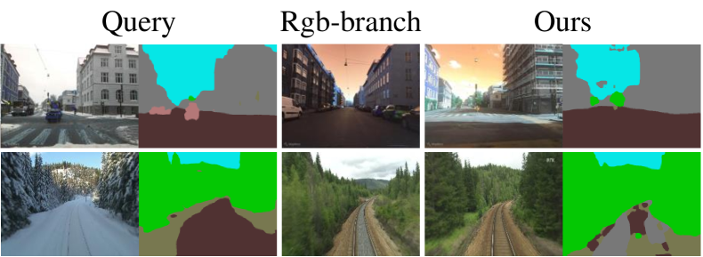
Figure 5: Qualitative results. In these examples, StructVPR successfully retrieves matching reference images, while rgb-branch produces incorrect place matches.

Table 4: Comparison to other fusion solutions on MSLS. Extraction latency includes the time to generate segmentation images.

Arch	MSLS val			MSLS challenge			Extraction
	R@1	R@5	R@10	R@1	R@5	R@10	latency (ms)
SEG	67.7	80.0	83.1	43.4	58.9	65.8	4$+$385
RGB	75.8	85.3	87.3	55.1	71.9	76.4	2.25
Multi-task	75.3	86.2	88.7	56.8	72.3	77.1	2.25
C-feat	75.5	86.5	88.8	55.9	73.3	78.1	6.25$+$385
C-input	77.7	88.4	91.4	59.7	76.9	81.2	21.67$+$385
KD(Ours)	83.0	91.0	92.6	64.5	80.4	83.9	2.25

Fusion Solutions. In the preliminary empirical studies, it has been demonstrated that segmentation images benefit VPR, and many solutions can achieve the fusion of two modalities in global retrieval. Here we give several feasible solutions and compare them:

• Concat-input: Concatenate RGB image and encoded segmentation label map in channel $C$ as input and train the model. Segmentation is required during testing.

• Concat-feat: Two feature vectors from two separate models are concatenated into a global feature. Segmentation is required during testing.

• Multi-task: Use the encoder-decoder structure, share the encoder with two tasks, and use the segmentation map as the supervision of the decoder. Segmentation is not required during testing.

• Knowledge distillation (Ours): Segmentation is not required during testing.

We train and compare them on MSLS and count the extraction latency during testing. Extraction latency is the time to obtain global features from a single RGB image.

As shown in Table 4, all fusion algorithms perform better than the two separate branches (RGB, SEG) on the MSLS dataset. But the performance of Concat-feat is limited, which may be due to a lack of coherence between two modalities. Although both Concat-input and KD perform relatively well, Concat-input requires additional processing of segmentation images during testing and has a larger model compared with KD. Neither Multi-task nor KD use segmentation images during testing. However, it is worth noting that the training of Multi-task has high requirements for parameter tuning, and KD is more direct and interpretable than Multi-task. Here we qualitatively demonstrate the advantages that StructVPR brings in Figure 5.

Segmentation label map encoding. The number of original semantic labels of the open-source model is 150. In Section 3.2, we use an encoding function to convert segmentation images into weighted one-hot label maps. Considering that $C$ and the prior weight setting are the most important hyper-parameters for our work, we perform ablation experiments on them. We also test $C=3,150$ in seg-branch for the number of clustered classes. After clustering, the redefined 3 categories are {sky&ground, dynamic objects, and static objects}. In addition, we present the results of different prior weight settings for $C=6$.

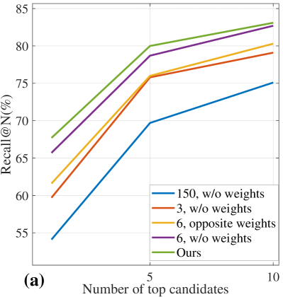
(a)

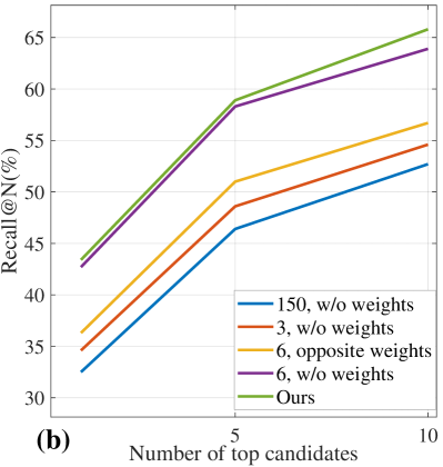
(b)

Figure 6: Performance of seg-branch with different number of clustered classes on (a) MSLS val. and (b) MSLS test dataset.

Figure 6 shows the results on the MSLS dataset. It can be seen that a too-small value of $C$ is not advisable, which will lose the uniqueness of the scene in our view, and the final performance is poor when $C=150$, which means that too fine-grained segmentation makes training more difficult. Finally, $C$ is set as 6. $\dagger$ stands for the opposite weight configuration: 0.5 for static objects and other objects, 2 for dynamic objects and vegetation. Comparing the results of unweighted and two weighted cases, we can qualitatively conclude that introducing appropriate prior weights can guide the model to converge better. Further analysis on prior weights is presented in the Supplementary Material.

Group partition strategy and the impact of groups. This paper proposes that not all samples are helpful in distillation and selects samples by group partitioning. At the same time, we propose using two pre-trained branches to participate in group partition together, instead of just using a separate one, to improve the accuracy of group partition and further achieve more accurate weighted KD. In this experiment, we perform selective KD to verify the importance of each group, which is a degenerate version of weighting for samples. In our expectation, samples of different groups should have different effects on distillation.

We compare our standard partition strategy (GP-D) with two degenerate configurations, as shown in Figure 7:

• Group partition with seg-branch (GP-S). Only the teacher network participates in the group partition.

• Group partition with rgb-branch (GP-R). Only the student network participates in the group partition.

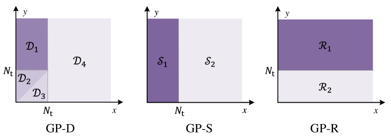
Figure 7: Visualization of different group partition strategies. Compared with our strategy (GP-D), which uses two models, both GP-S and GP-R have only one model involved in the partition.

Table 5: Performance of selective distillation with different samples. None refers to the rgb-branch without distillation and All refers to non-selective distillation.

Group for distillation	Sample ratio	MSLS val			MSLS challenge
		R@1	R@5	R@10	R@1	R@5	R@10
None	0%	75.8	85.3	87.3	55.1	71.9	76.4
All	100%	78.4	87.4	90.1	59.1	73.5	79.3
${\mathcal{D}_{1}}$	4.11%	78.8	89.2	91.1	62.3	76.8	80.9
${\mathcal{D}_{2}}$	50.67%	80.0	88.8	90.6	59.1	75.5	79.3
${\mathcal{D}_{3}}$	14.77%	77.7	87.4	89.2	57.8	74.4	79.1
${\mathcal{S}_{1}}$	69.55%	81.6	88.9	91.2	62.2	77.2	82.0
${\mathcal{S}_{2}}({\mathcal{D}_{4}})$	30.45%	71.6	83.7	85.1	48.2	63.9	68.7
${\mathcal{R}_{1}}$	73.24%	79.3	87.6	88.9	57.0	74.1	78.2
${\mathcal{R}_{2}}$	26.76%	73.8	82.7	85.6	51.0	67.0	72.3
Ours	69.55%	83.0	91.0	92.6	64.5	80.4	83.9

For selective KD, GP-D uses samples belonging to $\{{\mathcal{D}_{1}},{\mathcal{D}_{2}},{\mathcal{D}_{3}}\}$, GP-R uses $\{{\mathcal{S}_{1}}\}$, and GP-S uses $\{{\mathcal{R}_{1}}\}$. The meaning of ${\mathcal{S}_{1}},{\mathcal{S}_{1}},{\mathcal{S}_{1}},{\mathcal{S}_{1}}$ can refer to Section 3.4.

As shown in Table 5, we select a single group, in turn, to participate in distillation and evaluate its effectiveness. The results show that ${\mathcal{S}_{2}}$ and ${\mathcal{R}_{2}}$ harm distillation and other groups have different degrees of positive impact. All stands for non-selective KD using all samples in KD. However, its results are not as good as ${\mathcal{S}_{1}}$ and ${\mathcal{D}_{1}}$, indicating that the quality of samples is as important as the quantity for KD. So it is necessary to select suitable samples in distillation.

In this experiment, GP-S performs better than GP-R, and GP-D degenerates to GP-S. Furthermore, our partitioning strategy will show a considerable advantage over GP-S in weighted knowledge distillation.

Weighting distillation loss. We compare our weighting function (Eq. (4)) with constant weights to illustrate the importance of fine-grained weight assignment for samples. We have verified the importance of the groups above, which guides the design Eq. (4). The more essential samples for distillation, the higher the weight.

To further illustrate the advantages of GP-D, we also compare GP-D and GP-S with weighting functions. For GP-S, Eq. (4) degenerates into the following form:

$$\varphi^{\prime}(q,p)=\\ \begin{cases}1+\frac{1}{4\cdot\ln\left(1+RN_{s}\right)},&(q,p)\in{\mathcal{S}_{1}}\\ 0,&(q,p)\in{\mathcal{S}_{2}}\end{cases},$$ (7)

where the performance gap between the student network and the teacher network cannot be reflected on samples.

Table 6: Performance of weighted distillation with different weights. The weights correspond to $\mathcal{S}_{1}$-$\mathcal{S}_{2}$ and $\mathcal{D}_{1}$-$\mathcal{D}_{2}$-$\mathcal{D}_{3}$-$\mathcal{D}_{4}$, and GP-S(1-0) is equal to GP-D(1-1-1-0).

Weight	MSLS val			MSLS challenge
	R@1	R@5	R@10	R@1	R@5	R@10
GP-S(1-0)	81.6	88.9	91.2	62.2	77.2	82.0
GP-D(8-4-1-0)	82.2	88.9	91.5	62.3	78.9	82.4
GP-S($\varphi^{\prime}(q,p)$)	79.7	89.5	92.0	62.7	78.4	83.7
GP-D($\varphi(q,p)$)	83.0	91.0	92.6	64.5	80.4	83.9

In Table 6, GP-D(8-4-1-0) performs better than GP-S(1-0), and GP-D($\varphi(q,p)$) is better than GP-S($\varphi^{\prime}(q,p)$), which illustrate the importance of precise partition. Moreover, for both GP-D and GP-S, the weight function performs better than the discrete constant weights, respectively, showing the advantages of setting weights for each sample.

5 Discussion

Conclusion. In this paper, we address the problem of using segmentation information to enhance the structural knowledge in RGB global representations, attempting to replace the re-ranking process. To avoid the computation of segmentation during testing, we use the framework of knowledge distillation. We find that the teacher’s knowledge is not the more, the better; samples have different impacts on knowledge distillation, and some are even harmful. So we propose a weighted knowledge distillation method to partition samples and weigh the distillation loss for each sample. Experimental results show that StructVPR achieves SOTA performance among methods with only RGB global retrieval. Compared with two-stage methods, it is competitive with a better balance of accuracy and computation.

Limitations and Future Work. Nevertheless, some challenges remain. The clustered number and encoding values of semantic labels are chosen from five settings (Figure 6), and it calls for further advancements (details in appendix). Considering the robustness of StructVPR to SLME, smaller SEG models can be used to reduce costs. Furthermore, we believe that StructVPR is applicable to other tasks or modalities as long as multi-modal information is complementary at the sample level for tasks.

References

- [1] Relja Arandjelovic, Petr Gronat, Akihiko Torii, Tomas Pajdla, and Josef Sivic. NetVLAD: Cnn architecture for weakly supervised place recognition. In CVPR, pages 5297–5307, 2016.
- [2] Taichi Asami, Ryo Masumura, Yoshikazu Yamaguchi, Hirokazu Masataki, and Yushi Aono. Domain adaptation of dnn acoustic models using knowledge distillation. In ICASSP, pages 5185–5189, 2017.
- [3] Assia Benbihi, Stéphanie Arravechia, Matthieu Geist, and Cédric Pradalier. Image-based place recognition on bucolic environment across seasons from semantic edge description. In IEEE Int. Conf. Robot. Autom., pages 3032–3038, 2020.
- [4] Cristian Buciluǎ, Rich Caruana, and Alexandru Niculescu-Mizil. Model compression. In ACM SIGKDD, pages 535–541, 2006.
- [5] Luis G Camara and Libor Přeučil. Visual place recognition by spatial matching of high-level cnn features. Robot. Autom. Syst., 133:103625, 2020.
- [6] Bingyi Cao, Andre Araujo, and Jack Sim. Unifying deep local and global features for image search. In ECCV, pages 726–743, 2020.
- [7] Guobin Chen, Wongun Choi, Xiang Yu, Tony Han, and Manmohan Chandraker. Learning efficient object detection models with knowledge distillation. NeurIPS, 30, 2017.
- [8] Zetao Chen, Adam Jacobson, Niko Sünderhauf, Ben Upcroft, Lingqiao Liu, Chunhua Shen, Ian Reid, and Michael Milford. Deep learning features at scale for visual place recognition. In IEEE Int. Conf. Robot. Autom., pages 3223–3230, 2017.
- [9] Rui Dai, Srijan Das, and François Bremond. Learning an augmented rgb representation with cross-modal knowledge distillation for action detection. In ICCV, pages 13053–13064, 2021.
- [10] Daniel DeTone, Tomasz Malisiewicz, and Andrew Rabinovich. Superpoint: Self-supervised interest point detection and description. In CVPR, pages 224–236, 2018.
- [11] Mihai Dusmanu, Ignacio Rocco, Tomas Pajdla, Marc Pollefeys, Josef Sivic, Akihiko Torii, and Torsten Sattler. D2-net: A trainable cnn for joint description and detection of local features. In CVPR, pages 8092–8101, 2019.
- [12] Nuno C Garcia, Pietro Morerio, and Vittorio Murino. Modality distillation with multiple stream networks for action recognition. In ECCV, pages 103–118, 2018.
- [13] Abel Gawel, Carlo Del Don, Roland Siegwart, Juan Nieto, and Cesar Cadena. X-view: Graph-based semantic multi-view localization. Robot. Autom. lett., 3(3):1687–1694, 2018.
- [14] Shiming Ge, Shengwei Zhao, Chenyu Li, and Jia Li. Low-resolution face recognition in the wild via selective knowledge distillation. IEEE TIP, 28(4):2051–2062, 2018.
- [15] Yixiao Ge, Haibo Wang, Feng Zhu, Rui Zhao, and Hongsheng Li. Self-supervising fine-grained region similarities for large-scale image localization. In ECCV, pages 369–386, 2020.
- [16] Albert Gordo, Jon Almazan, Jerome Revaud, and Diane Larlus. End-to-end learning of deep visual representations for image retrieval. IJCV, 124(2):237–254, 2017.
- [17] Jianping Gou, Baosheng Yu, Stephen J Maybank, and Dacheng Tao. Knowledge distillation: A survey. IJCV, 129(6):1789–1819, 2021.
- [18] Saurabh Gupta, Judy Hoffman, and Jitendra Malik. Cross modal distillation for supervision transfer. In CVPR, pages 2827–2836, 2016.
- [19] Miao Hao, Yitao Liu, Xiangyu Zhang, and Jian Sun. Labelenc: A new intermediate supervision method for object detection. In ECCV, pages 529–545, 2020.
- [20] Stephen Hausler, Sourav Garg, Ming Xu, Michael Milford, and Tobias Fischer. Patch-NetVLAD: Multi-scale fusion of locally-global descriptors for place recognition. In CVPR, pages 14141–14152, 2021.
- [21] Geoffrey Hinton, Oriol Vinyals, Jeff Dean, et al. Distilling the knowledge in a neural network. arXiv preprint arXiv:1503.02531, 2(7), 2015.
- [22] Judy Hoffman, Saurabh Gupta, and Trevor Darrell. Learning with side information through modality hallucination. In CVPR, pages 826–834, 2016.
- [23] Hanjiang Hu, Zhijian Qiao, Ming Cheng, Zhe Liu, and Hesheng Wang. Dasgil: Domain adaptation for semantic and geometric-aware image-based localization. IEEE TIP, 30:1342–1353, 2020.
- [24] Ahmad Khaliq, Shoaib Ehsan, Zetao Chen, Michael Milford, and Klaus McDonald-Maier. A holistic visual place recognition approach using lightweight cnns for significant viewpoint and appearance changes. IEEE Trans. Robot., 36(2):561–569, 2019.
- [25] Alex Krizhevsky, Ilya Sutskever, and Geoffrey E Hinton. Imagenet classification with deep convolutional neural networks. NeurIPS, 25:1097–1105, 2012.
- [26] Jinyu Li, Michael L Seltzer, Xi Wang, Rui Zhao, and Yifan Gong. Large-scale domain adaptation via teacher-student learning. arXiv preprint arXiv:1708.05466, 2017.
- [27] Shining Liang, Ming Gong, Jian Pei, Linjun Shou, Wanli Zuo, Xianglin Zuo, and Daxin Jiang. Reinforced iterative knowledge distillation for cross-lingual named entity recognition. In ACM SIGKDD, pages 3231–3239, 2021.
- [28] Stephanie Lowry, Niko Sünderhauf, Paul Newman, John J Leonard, David Cox, Peter Corke, and Michael J Milford. Visual place recognition: A survey. IEEE Trans. Robot., 32(1):1–19, 2015.
- [29] Feng Lu, Baifan Chen, Xiang-Dong Zhou, and Dezhen Song. STA-VPR: Spatio-temporal alignment for visual place recognition. Robot. Autom. lett., 6(3):4297–4304, 2021.
- [30] Carlo Masone and Barbara Caputo. A survey on deep visual place recognition. IEEE Access, 9:19516–19547, 2021.
- [31] Eva Mohedano, Kevin McGuinness, Noel E O’Connor, Amaia Salvador, Ferran Marques, and Xavier Giró-i Nieto. Bags of local convolutional features for scalable instance search. In ACM Int. Conf. Multimedia Retr, pages 327–331, 2016.
- [32] Hyeonwoo Noh, Andre Araujo, Jack Sim, Tobias Weyand, and Bohyung Han. Large-scale image retrieval with attentive deep local features. In ICCV, pages 3456–3465, 2017.
- [33] Daniel Olid, José M Fácil, and Javier Civera. Single-view place recognition under seasonal changes. arXiv preprint arXiv:1808.06516, 2018.
- [34] Valerio Paolicelli, Antonio Tavera, Carlo Masone, Gabriele Berton, and Barbara Caputo. Learning semantics for visual place recognition through multi-scale attention. In Int. Conf. Image Anal. Process., pages 454–466, 2022.
- [35] Guohao Peng, Yufeng Yue, Jun Zhang, Zhenyu Wu, Xiaoyu Tang, and Danwei Wang. Semantic reinforced attention learning for visual place recognition. In IEEE Int. Conf. Robot. Autom., pages 13415–13422, 2021.
- [36] Nathan Piasco, Désiré Sidibé, Valérie Gouet-Brunet, and Cédric Demonceaux. Learning scene geometry for visual localization in challenging conditions. In IEEE Int. Conf. Robot. Autom., pages 9094–9100, 2019.
- [37] Nathan Piasco, Désiré Sidibé, Valérie Gouet-Brunet, and Cédric Demonceaux. Improving image description with auxiliary modality for visual localization in challenging conditions. IJCV, 129(1):185–202, 2021.
- [38] Filip Radenović, Giorgos Tolias, and Ondřej Chum. Fine-tuning cnn image retrieval with no human annotation. IEEE TPAMI, 41(7):1655–1668, 2018.
- [39] Sucheng Ren, Yong Du, Jianming Lv, Guoqiang Han, and Shengfeng He. Learning from the master: Distilling cross-modal advanced knowledge for lip reading. In CVPR, pages 13325–13333, 2021.
- [40] Jerome Revaud, Jon Almazán, Rafael S Rezende, and Cesar Roberto de Souza. Learning with average precision: Training image retrieval with a listwise loss. In ICCV, pages 5107–5116, 2019.
- [41] Mark Sandler, Andrew Howard, Menglong Zhu, Andrey Zhmoginov, and Liang-Chieh Chen. Mobilenetv2: Inverted residuals and linear bottlenecks. In CVPR, pages 4510–4520, 2018.
- [42] Paul-Edouard Sarlin, Cesar Cadena, Roland Siegwart, and Marcin Dymczyk. From coarse to fine: Robust hierarchical localization at large scale. In CVPR, pages 12716–12725, 2019.
- [43] Paul-Edouard Sarlin, Daniel DeTone, Tomasz Malisiewicz, and Andrew Rabinovich. Superglue: Learning feature matching with graph neural networks. In CVPR, pages 4938–4947, 2020.
- [44] Florian Schroff, Dmitry Kalenichenko, and James Philbin. Facenet: A unified embedding for face recognition and clustering. In CVPR, pages 815–823, 2015.
- [45] René Schuster, Oliver Wasenmuller, Christian Unger, and Didier Stricker. Sdc-stacked dilated convolution: A unified descriptor network for dense matching tasks. In CVPR, pages 2556–2565, 2019.
- [46] Yanqing Shen, Ruotong Wang, Weiliang Zuo, and Nanning Zheng. Tcl: Tightly coupled learning strategy for weakly supervised hierarchical place recognition. Robot. Autom. lett., 7(2):2684–2691, 2022.
- [47] Niko Sünderhauf, Peer Neubert, and Peter Protzel. Are we there yet? challenging seqslam on a 3000 km journey across all four seasons. In IEEE Int. Conf. Robot. Autom. Worksh., page 2013, 2013.
- [48] Marvin Teichmann, Andre Araujo, Menglong Zhu, and Jack Sim. Detect-to-retrieve: Efficient regional aggregation for image search. In CVPR, pages 5109–5118, 2019.
- [49] Akihiko Torii, Josef Sivic, Tomas Pajdla, and Masatoshi Okutomi. Visual place recognition with repetitive structures. In CVPR, pages 883–890, 2013.
- [50] Fusheng Wang, Jianhao Yan, Fandong Meng, and Jie Zhou. Selective knowledge distillation for neural machine translation. In Int. Joint Conf. Natural Lang. Process., pages 6456–6466, 2021.
- [51] Ruotong Wang, Yanqing Shen, Weiliang Zuo, Sanping Zhou, and Nanning Zheng. Transvpr: Transformer-based place recognition with multi-level attention aggregation. In CVPR, pages 13648–13657, 2022.
- [52] Frederik Warburg, Soren Hauberg, Manuel Lopez-Antequera, Pau Gargallo, Yubin Kuang, and Javier Civera. Mapillary street-level sequences: A dataset for lifelong place recognition. In CVPR, pages 2626–2635, 2020.
- [53] Yu-Huan Wu, Yun Liu, Jun Xu, Jia-Wang Bian, Yu-Chao Gu, and Ming-Ming Cheng. Mobilesal: Extremely efficient rgb-d salient object detection. IEEE TPAMI, 2021.
- [54] Xiwu Zhang, Lei Wang, and Yan Su. Visual place recognition: A survey from deep learning perspective. Pattern Recognition, 113:107760, 2021.
- [55] Long Zhao, Xi Peng, Yuxiao Chen, Mubbasir Kapadia, and Dimitris N Metaxas. Knowledge as priors: Cross-modal knowledge generalization for datasets without superior knowledge. In CVPR, pages 6528–6537, 2020.
- [56] Sanping Zhou, Fei Wang, Zeyi Huang, and Jinjun Wang. Discriminative feature learning with consistent attention regularization for person re-identification. In ICCV, pages 8040–8049, 2019.
- [57] Sanping Zhou, Jinjun Wang, Deyu Meng, Yudong Liang, Yihong Gong, and Nanning Zheng. Discriminative feature learning with foreground attention for person re-identification. IEEE TIP, 28(9):4671–4684, 2019.
- [58] Sanping Zhou, Jinjun Wang, Jiayun Wang, Yihong Gong, and Nanning Zheng. Point to set similarity based deep feature learning for person re-identification. In CVPR, pages 3741–3750, 2017.