First-Order Methods for Nonsmooth Nonconvex Functional Constrained Optimization with or without Slater Points

Abstract

Constrained optimization problems where both the objective and constraints may be nonsmooth and nonconvex arise across many learning and data science settings. In this paper, we show a simple first-order method finds a feasible, $\epsilon$-stationary point at a convergence rate of $O(\epsilon^{-4})$ without relying on compactness or Constraint Qualification (CQ). When CQ holds, this convergence is measured by approximately satisfying the Karush–Kuhn–Tucker conditions. When CQ fails, we guarantee the attainment of weaker Fritz-John conditions. As an illustrative example, our method stably converges on piecewise quadratic SCAD regularized problems despite frequent violations of constraint qualification. The considered algorithm is similar to those of [1, 2] (whose guarantees further assume compactness and CQ), iteratively taking inexact proximal steps, computed via an inner loop applying a switching subgradient method to a strongly convex constrained subproblem. Our non-Lipschitz analysis of the switching subgradient method appears to be new and may be of independent interest.

1 Introduction

In this paper, we considered the difficult family of constrained optimization problems where both the objective and constraints may be nonconvex and nonsmooth. Specifically, we consider problems of the following form:

$$\begin{cases}\min_{x\in X}\quad&f(x)\\ \mathrm{s.t.}\quad&g_{i}(x)\leq 0,\qquad i=1,...,m.\end{cases}$$ (1.1)

for some closed convex domain $X\subseteq\mathbb{R}^{d}$. The objective $f:X\to\mathbb{R}$ and constraints $g_{i}:X\to\mathbb{R},i=1,...,m$ are assumed to be continuous on $X$, but need not be convex nor differentiable.

Constrained optimization problems with nonsmooth and nonconvex objective loss functions and constraints are common in modern data science and machine learning. For instance, phase retrieval, blind deconvolution, and covariance matrix estimation all fall within nonconvex and nonsmooth minimization [3, 4, 5, 6, 7]. If sparsity of solutions is expected or desired, often a regularizing constraint is introduced (e.g., convex choices like $\ell_{1}$-norms or $\ell_{2}$-norms, nonconvex choices like SCAD functions [8, 9] or $\ell_{q}$-norms for $q\in(0,1)$). SCAD functions will serve as a running example throughout this work as they are simple piecewise quadratic functions exhibiting nonsmoothness and nonconvexity, with widespread usage [10, 11, 12, 13, 14]. Other problems like multi-class Neyman-Pearson classification [15, 1, 16], minimizing the loss on one class while controlling the losses on other classes under some values, provide another typical setting of constrained optimization inheriting any nonsmoothness and nonconvexities from the loss functions.

Our approach to solving nonsmooth, nonconvex, constrained problems relies on two main ingredients outlined below: (in)exact proximal point methods and Fritz-John/Karush-Kuhn-Tucker stationarity conditions.

(In)exact Proximal Point Methods

Several recent works [17, 18, 19, 20, 7, 21] have concerned solving nonconvex problems via inexact evaluation of a proximal operator. For settings without functional constraints (i.e., $m=0$), these methods seek a stationary point of $\min_{x\in X}f(x)$ by iterating

$$x_{k+1}\approx\text{prox}_{\alpha,f}(x_{k}):=\operatornamewithlimits{argmin}_{x\in X}\left\{f(x)+\frac{1}{2\alpha}\|x-x_{k}\|^{2}\right\}$$ (1.2)

with stepsize $\alpha>0$. By restricting to the family of weakly convex functions (defined in (2.4)), this proximal subproblem is guaranteed to be convex with a unique solution for small enough $\alpha$. When the proximal map can be evaluated exactly, an $\epsilon>0$-stationary point (defined in Definitions 2.1 and 2.2) is found within $O(1/\epsilon^{2})$ iterations. The inexact methods of [21, 7] show that using cheaper subgradient oracle calls such a point is found within $O(1/\epsilon^{4})$ iterations.

We follow the extension of these ideas to nonconvex inequality constraints proposed by Ma et al [1] and Boob et al [2]. Their ideas and comparisons with our contributions are discussed in Section 1.3. To this end, we consider the following proximal subproblem, penalizing the constraints in addition to the objective

$$x_{k+1}\approx\operatornamewithlimits{argmin}_{x\in X}\left\{f(x)+\frac{1}{2\alpha}\|x-x_{k}\|^{2}\mid g_{i}(x)+\frac{1}{2\alpha}\|x-x_{k}\|^{2}\leq\tau\right\}$$ (1.3)

with stepsize $\alpha>0$ and feasibility tolerance $\tau\geq 0$. Importantly, any feasible solution to this proximal subproblem $x_{k+1}$ has its infeasibility bounded by $g_{i}(x_{k+1})\leq\tau-\frac{1}{2\alpha}\|x_{k}-x_{k+1}\|^{2}_{2}$. Hence a sequence of $x_{k}$ generated by inexactly evaluating this mapping remains feasible for the original problem (1.1) until it reaches approximate stationarity (that is, $\|x_{k}-x_{k+1}\|_{2}\geq\sqrt{2\alpha\tau}$ implies $g_{i}(x_{k+1})\leq 0$ for each constraint $i$).

Fritz-John/Karush-Kuhn-Tucker Stationarity

Let $\partial f(x)$ denote a generalized subdifferential of a function $f$ and $N_{X}(x)$ denote the normal cone of $X$ at $x$, formally defined in Section 2. Here we consider two classic measurements of stationarity: Fritz-John (FJ) conditions giving a weaker optimality condition and Karush-Kuhn-Tucker (KKT) conditions giving a stronger condition.

We say that a feasible solution $x^{*}$ is a FJ point of (1.1) if there exists nonnegative multipliers $\gamma_{0}^{*}\in\mathbb{R}$ and $\gamma^{*}=(\gamma_{1}^{*},...,\gamma_{m}^{*})^{T}\in\mathbb{R}^{m}$, and subgradients $\zeta_{f}\in\partial f(x^{*})$ and $\zeta_{gi}\in\partial g_{i}(x^{*})$ such that $(\gamma_{0}^{*},\gamma_{1}^{*},...,\gamma_{m}^{*})$ is a non-zero vector with

$$\gamma_{i}^{*}g_{i}(x^{*}) =0,\qquad\forall i=1,...,m,$$ (1.4)

$$\gamma_{0}^{*}\zeta_{f}+\sum_{i=1}^{m}\gamma_{i}^{*}\zeta_{gi} \in-N_{X}(x^{*}).$$

Note requiring $(\gamma_{0}^{*},\gamma_{i}^{*},...,\gamma_{m}^{*})$ to be a nonzero vector could be equivalently expressed as requiring $\gamma_{0}^{*}+\sum_{i=1}^{m}\gamma_{i}^{*}=1$. This condition is necessary for $x^{*}$ to be a global (or local) minimizer [22]. However, this condition can only give limited insights into the quality of $x^{*}$ as a solution when $\gamma_{0}^{*}=0$ since (1.4) becomes independent of $f$ [23]. This weakness is remedied by the stronger notion of KKT points, which implicitly require $\gamma_{0}^{*}\neq 0$. We say a feasible $x^{*}$ is a KKT point for the problem (1.1) if there exists nonnegative Lagrange multipliers $\lambda^{*}\in\mathbb{R}^{m}$, $\zeta_{f}\in\partial f(x^{*})$ and $\zeta_{gi}\in\partial g_{i}(x^{*})$ such that

$$\lambda_{i}^{*}g_{i}(x^{*}) =0,\qquad\forall i=1,...,m,$$ (1.5)

$$\zeta_{f}+\sum_{i=1}^{m}\lambda_{i}^{*}\zeta_{gi} \in-N_{X}(x^{*}).$$

The KKT conditions strengthen FJ, requiring $\gamma_{0}^{*}\neq 0$, in particular $\gamma_{0}^{*}=1$. The requirement that $\gamma_{0}^{*}\neq 0$ is equivalent to having the Mangasarian-Fromovitz Constraint Qualification (MFCQ) condition hold: Let $A(x)=\{i\mid g_{i}(x)=0,i=1,...,m\}$. We say MFCQ holds at $x^{*}$ if

$$\exists v\in-N_{X}^{*}(x^{*})\qquad s.t.\quad\zeta_{gi}^{T}v<0\quad\forall i\in A(x),\forall\zeta_{gi}\in\partial g_{i}(x^{*}).$$ (1.6)

Approximate FJ and KKT stationarity measurements can differ greatly when constraint qualification does not hold. When a strengthened ($\sigma$-strong) MFCQ condition (defined later as (2.9)) is satisfied, we can uniformly bound the size of any associated Lagrange multipliers. Without this, these multipliers may be arbitrarily large, even failing to exist when MFCQ fails. Consequently, approximate KKT stationarity may never be attained despite the iterates $x_{k}$ of (1.3) converging. In contrast, we show that the FJ conditions are approximately satisfied whenever $x_{k}$ converges.

1.1 Contribution

We show that an inexact proximal method can solve a wide range of nonsmooth, nonconvex constrained optimization problems, producing an approximate stationary point using at most $O(1/\epsilon^{4})$ subgradient evaluations, matching its rate for unconstrained optimization. In particular, our proposed method uses a switching subgradient method approximately solving (1.3) to produce each subsequent $x_{k+1}$, see Algorithm 1. Our analysis shows the following three generally desirable properties missing from prior works [1, 2]:

Always Feasible Iterates

By appropriately selecting the algorithmic parameters, we can ensure feasibility $g_{i}(x_{k+1})\leq 0$ at each iteration. Maintaining not just approximately but actually feasible iterates is critical, for example, in settings of planning or control where feasibility corresponds to physical limitations or safety concerns [24, 25].

Stationarity with or without Constraint Qualification

Ensuring constraint qualification over nonconvex constraints is nontrivial, despite being continually assumed by prior works. This is illustrated for a common sparse regularizer in Section 1.2 and numerical explored in Section 5. In Theorems 3.2 and 3.3, we show that at most $O(1/\epsilon^{4})$ subgradient evaluations are required to produce an approximate KKT or FJ point, with or without constraint qualification, respectively.

Convergence Rates without Compactness

Our guarantees apply without needing to assume compactness of the domain $X$, which prior works relied on. Hence our theory applies more widely and, even in compact settings, may offer improvements as quantities like the diameter of $X$ are replaced by often smaller quantities dependent on the initialization. This is done by extending the analysis of the switching subgradient method to handle non-Lipschitz objective and constraint functions like those occurring in (1.3). This analysis and resulting subproblem convergence guarantee appear to be new and may be of independent interest.

1.2 Vignette: Failure of MFCQ Assumptions for Sparse Regularized Problems

Nonconvex regularization has recently gained popularity due to its ability to facilitate stronger statistical guarantees on minimizers [26, 27, 28, 29]. One of the simplest regularizers is the Smoothly Clipped Absolute Deviation (SCAD) function [8, 9], which sums up piecewise quadratic clipped absolute deviations in each coordinate

$$s(x_{i})=\begin{cases}2|x_{i}|&{0\leq|x_{i}|\leq 1},\\ -x_{i}^{2}+4|x_{i}|-1&{1<|x_{i}|\leq 2},\\ 3&{|x_{i}|>2}.\end{cases}$$ (1.7)

Near the origin, this behaves like a one-norm. As larger points are considered, it smoothly flattens out to overly penalizing large entries. Figure 1(a) shows the one-dimensional SCAD function. Note the constraint $g(x):=\sum_{i}s(x_{i})-p\leq 0$ ensures that at most $\lfloor p/3\rfloor$ entries of $x$ have a magnitude larger than two. Figure 1(b) shows the feasible regions given by the three-dimensional SCAD constraints in $[-5,5]^{3}$.

Optimization over these level sets will often yield sparse solutions, guaranteed to have no more than $\lfloor p/3\rfloor$ entries greater than 2. Since SCAD constraints are piecewise quadratic, we can often approximately solve the convex subproblem (1.3). Despite this, two problems (one mild and one severe) prevent applying the convergence theory of prior works.

First, prior works do not apply as the set $\{x\mid g(x)\leq 0\}$ is not compact for any $p\geq 3$. If a bound on the size of a solution is known, then one could add a ball constraint $X=\{x\mid\|x\|\leq D\}$ to ensure compactness. Our theory applies without such a modification.

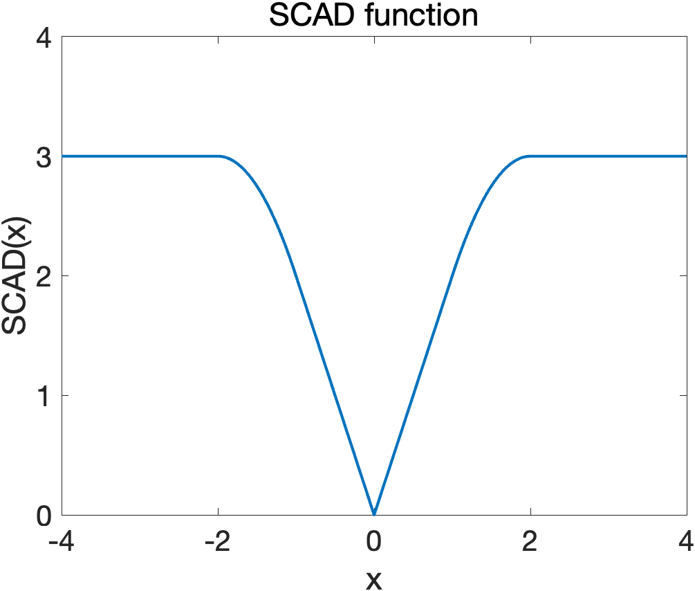
((a)) $1$D SCAD function

((b)) Seven SCAD level sets with $p\in\{2.5,3.5,4.5,5.5,6.5,7.5,8.5\}$. Note the set changes suddenly at $p\in\{3,6,9\}$, where MFCQ fails.

Figure 1: The SCAD function $s$ and feasible regions in 3D given by $\sum_{i}s(x_{i})\leq p$.

((a)) Small values of $p$

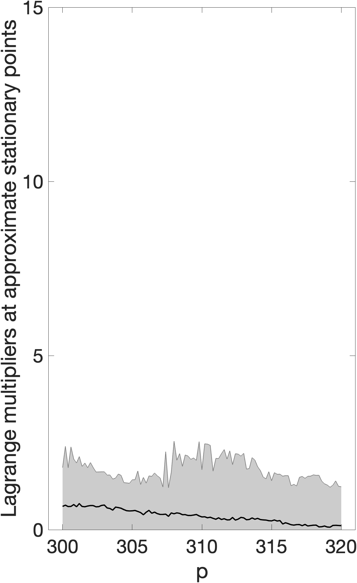
((b)) Large values of $p$

Figure 2: Lagrange multipliers computed at approximate stationary points reached by iterating (1.3) on $30$ randomly generated SPR problems (see Section 5 for the exact construction). As $p$ varies from $60$ to $120$, the black line shows the average approximate multipliers reached and the gray region shows the range between maximum and minimum values seen. Black dots are placed at each multiple of three, where MFCQ fails to hold.

More subtly, prior works do not apply here as SCAD constraints often fail to have constraint qualification hold as $p$ varies. As a result, none of the prior works’ theories provide any form of convergence guarantee. To illustrate this, we numerically consider the problem of Sparse Phase Retrieval problems (SPR), see (5.1), which minimizes a piecewise quadratic objective over the piecewise quadratic constraint set for SCAD constraints. Figure 2 shows the estimated Lagrange multipliers at limit points converged to by an inexact proximal point method. When $p$ is near a multiple of three, the limit point reached by iteratively applying (1.3) may fail to satisfy MFCQ, seen as its associated Lagrange multiplier blowing up, preventing KKT attainment. For large values of $p$, we see the multipliers tending to zero, corresponding to unconstrained stationarity.

Despite these failures of MFCQ, our theory still guarantees that the iteration will find an approximate FJ point. Note that Figure 2 is based on averaging $30$ independent replicates. We only observe approximately $5\%\sim 10\%$ of replicates when $p$ is a multiple of three have their Lagrange multipliers diverge. So MFCQ is often violated but not everywhere. These sporadic failures in relatively simple nonsmooth nonconvex settings are one of this work’s original motivations, leading us to develop theory capable of describing convergence when MFCQ fails while retaining (and improving) the convergence theory when MFCQ holds.

1.3 Related Work

Inexact Proximal Methods

Using inexact proximal-point methods to solve nonsmooth nonconvex problems is not new to this work. Double-loop algorithms that use several inner steps to inexactly solve a convex proximal subproblem in each outer iteration have been designed and analyzed widely. For example, the algorithm proposed in [17] approximating nonconvex proximal points contributed to such an idea, and [18] presented a proximal variant of bundle methods solving nonconvex problems based on the work of [17]. More recently, [21] developed this idea to give a $O(1/\epsilon^{4})$ convergence rate for unconstrained stochastic nonsmooth nonconvex problems.

Special Case of (Strongly) Convex Constraints

A range of methods from the literature can be applied to inexactly solve the nonsmooth but strongly convex constrained subproblems constructed, which here arise as the subproblems (2.12). A level-set method for structured convex constrained problems was introduced in [30], which was generalized and improved by [31] to maintain feasibility. Alternative (augmented) Lagrangian approaches could be applied if near feasibility is sufficient. Here we take the approach of solving such problems via switching subgradient methods, which have been analyzed in [32] and extended in [1], [33] and [34].

Comparison with Ma, Lin, and Yang [1]

We consider a very similar inexact proximal point method with switching subgradient method being the oracle for the subproblems as Ma et al. [1], in which they also find nearly optimal and nearly feasible solutions for the subproblems. Their work also analyzed the convergence of a stochastic subgradient algorithm. However, in the deterministic setting, they only guarantee nearly feasible and approximate stationary solutions for the original optimization problem, while our method ensures actual feasibility. To attain KKT stationarity, they introduced a uniform Slater’s condition as their stronger type of constraint qualification, which is stronger than our considered $\sigma$-strong MFCQ condition. Moreover, their upper bound on the optimal dual variables and convergence rates depend on the diameter of $X$, while we do not need such a requirement. Up to these constants, Ma et al. proved a $O(\epsilon^{-4})$ rate of convergence towards KKT guarantees under MFCQ, which we match (in addition to our new FJ guarantees).

Comparison with Boob, Deng, and Lan [2]

As another closely related work, Boob et al. [2] showed that the inexact proximal point method searching for nearly optimal and strictly feasible solutions for the subproblems can ensure a feasible approximate stationary solution for the main problem is found (assuming $X$ is compact). This framework maintains strict feasibility automatically during the iterations. Our proposed method, although it also ensures feasibility, does not neatly fit within their framework of guaranteeing strict feasibility. Boob et al. consider problem settings ranging from nonconvex to strongly convex constrained problems and consider various MFCQ, strong MFCQ, and strong feasibility conditions as constraint qualifications. Their strong feasibility condition is stronger than our considered $\sigma$-strong MFCQ condition. Under their MFCQ and strong MFCQ conditions, an additional assumption is needed to ensure the existence of a stationary solution that the iterated points converge to and ensure boundedness of the optimal dual variables. They did not prove a constant limit on this upper bound, while we attain a closed form for this upper bound directly from strong MFCQ.

Prior Nonconvex Fritz John and KKT-type Guarantees

Birgin et al. [35] gave a general method that attains approximate stationarity using first, second, or higher-order information. They adopted both scaled KKT points and unscaled KKT points to describe the stationarity, where the former means the accuracy of KKT conditions satisfied at such points is proportional to the size of the Lagrange multipliers. Scaled KKT points with a linear combination of the gradients of the constraints being near zero are similar to FJ points. Hinder and Ye [36] showed that a (slightly modified) Fritz-John stationarity can be reached by an interior point method despite nonconvex constraints. They also introduced their new definitions of unscaled KKT points and termination criteria as comparisons with [35]. The ideas of adopting scaled KKT stationarity and discussions on its dependence on the size of Lagrange multipliers also occur in [37, 38, 39, 40].

Alternative Approaches to Nonconvex Constraints

Finally, we note three alternatives to the use of (inexact) proximal methods for nonconvex constrained problems considered here: Classic second-order approaches like sequential quadratic programming techniques [41] can be applied. Cubic regularization approaches [42] and penalized methods [43, 44] can also provide provably convergence guarantees. If the constraints are star convex with respect to a known point (for example, the SCAD constraints previously considered with respect to the origin), the radial methods of [45, 46] could apply with convergence guarantees while maintaining fully feasible iterates.

2 Preliminaries

Throughout the paper, we use the following notations. Let $\|\cdot\|$ denote the $l_{2}$-norm. We denote the normal cone of $X$ at $x$ as $N_{X}(x)$, and its dual cone as $N^{*}_{X}(x)$. The distance from a point $x$ to a set $S$ is denoted as ${\rm dist}(x,S)=\min_{s\in S}\|x-s\|$, and the convex hull of any set $S$ is denoted as $\mathrm{co}\{S\}$. For any convex function $h:X\to\mathbb{R}\cup\{+\infty\}$, its set of subgradients at $x\in X$ is defined as:

$$\partial h(x)=\{\zeta\in\mathbb{R}^{d}|h(x^{\prime})\geq h(x)+\zeta^{T}(x^{\prime}-x),\quad\forall x^{\prime}\in X\}.$$ (2.1)

More generally, for any potentially nonconvex function $h:X\to\mathbb{R}\cup\{+\infty\}$, its set of Clarke subgradients at $x$ is defined as:

$$\partial h(x)=\mathrm{co}\{\lim_{i\to\infty}\nabla h(x_{i})|x_{i}\to x\text{ and }h(x)\text{ is differentiable at any }x_{i}\in X\}.$$ (2.2)

A function $h(x)$ is $\mu$-strongly convex on $X$ if $h-\frac{\mu}{2}\|\cdot\|^{2}$ is convex. This is equivalent to having:

$$h(x^{\prime})\geq h(x)+\zeta^{T}(x^{\prime}-x)+\frac{\mu}{2}\|x^{\prime}-x\|^{2},\qquad\forall x,x^{\prime}\in X,\forall\zeta\in\partial h(x).$$ (2.3)

A function $h(x)$ is $\rho$-weakly convex on $X$ if $h+\frac{\rho}{2}\|\cdot\|^{2}$ is convex. This is equivalent to having:

$$h(x^{\prime})\geq h(x)+\zeta^{T}(x^{\prime}-x)-\frac{\rho}{2}\|x^{\prime}-x\|^{2},\qquad\forall x,x^{\prime}\in X,\forall\zeta\in\partial h(x).$$ (2.4)

We consider two different notions describing approximate stationarity for our nonsmooth nonconvex constrained problem of interest (1.1), weakening the FJ conditions and KKT conditions shown in (1.4) and (1.5) respectively.

Definition 2.1.

A point x is an $\epsilon$-FJ point for problem (1.1) if $g_{i}(x)\leq 0\ \forall i=1,...,m$, and there exists $\zeta_{f}\in\partial f(x)$, $\zeta_{gi}\in\partial g_{i}(x)$ and $\gamma_{0}\geq 0$, $\gamma=(\gamma_{1},...,\gamma_{m})^{T}\geq 0$, $\gamma_{0}+\sum_{i=1}^{m}\gamma_{i}=1$ such that:

$${\rm dist}(\gamma_{0}\zeta_{f}+\sum_{i=1}^{m}\gamma_{i}\zeta_{g},-N_{X}(x)) \leq\epsilon,$$ (2.5)

$$|\gamma_{i}g_{i}(x)| \leq\epsilon^{2}\qquad\forall i=1,...,m.$$ (2.6)

Definition 2.2.

A point x is an $\epsilon$-KKT point for problem (1.1) if $g_{i}(x)\leq 0\ \forall i=1,...,m$, and there exists $\zeta_{f}\in\partial f(x)$, $\zeta_{gi}\in\partial g_{i}(x)$ and $\lambda=(\lambda_{1},...,\lambda_{m})^{T}\geq 0$ such that:

$${\rm dist}(\zeta_{f}+\sum_{i=1}^{m}\lambda_{i}\zeta_{gi},-N_{X}(x)) \leq\epsilon,$$ (2.7)

$$|\lambda_{i}g_{i}(x)| \leq\epsilon^{2}\qquad\forall i=1,...,m.$$ (2.8)

Let $\hat{x}_{k+1}$ denote the optimal solution for the subproblem (1.3). The considered inexact proximal point approach will produce iterates $x_{k+1}$ near each $\hat{x}_{k+1}$. As we will see, the sequence $\hat{x}_{k}$ converges towards an approximate stationary point for the main problem (1.1). So we can only ensure our iterates $x_{k}$ are near an approximately stationary point. The following definitions describe points in the proximity of an approximately stationary point.

Definition 2.3.

A point x is an $(\epsilon,\eta)$-FJ point for problem (1.1) if there exists an $\epsilon$-FJ point $x^{\prime}$ for problem (1.1) with $\|x-x^{\prime}\|\leq\eta$.

Definition 2.4.

A point x is an $(\epsilon,\eta)$-KKT point for problem (1.1) if there exists an $\epsilon$-KKT point $x^{\prime}$ for problem (1.1) with $\|x-x^{\prime}\|\leq\eta$.

The accuracy of KKT stationarity guarantees we derive will depend on the sizes of the associated Lagrange multipliers. To give a constant upper bound on these optimal Lagrange multipliers in (1.5) for our subproblems (see problem (2.12) below), we assume a stronger type of constraint qualification defined below. Let $A(x)=\{i\mid g_{i}(x)=0,i=1,...,m\}$. We say $\sigma$-strong MFCQ condition holds at $x$ if there exists a constant $\sigma>0$, such that:

$$\exists v\in-N_{X}^{*}(x)\quad and\quad\|v\|=1\qquad s.t.\quad\zeta_{gi}^{T}v\leq-\sigma\quad\forall i\in A(x),\forall\zeta_{gi}\in\partial g_{i}(x).$$ (2.9)

Specifically, when $N_{X}(x)=\{\mathbf{0}\}$, we could equivalently state the condition as:

$$\|\zeta_{gi}\|\geq\sigma\quad\forall i\in A(x),\forall\zeta_{gi}\in\partial g_{i}(x).$$ (2.10)

We say the $\sigma$-strong MFCQ condition holds for problem (1.1) when $\sigma$-strong MFCQ condition is satisfied at any $x\in X$. When the $\sigma$-strong MFCQ condition is satisfied for all the subproblems (2.12), our Lemma 3.4 shows boundedness of Lagrange multipliers in (1.5) for our subproblems. This boundness is critical to improve our FJ convergence guarantees to convergence towards KKT stationarity.

Without loss of generality, we simplify the $m$ nonsmooth, nonconvex constraints of (1.1) into a single constraint as follows:

$$\begin{cases}\min_{x\in X}\quad&f(x)\\ \mathrm{s.t.}\quad&g(x):=\max_{i=1,...,m}g_{i}(x)\leq 0.\end{cases}$$ (2.11)

Note if each $g_{i}$ is $\rho$-weakly convex, then $g$ is $\rho$-weakly convex. Note that in this reformulation, there is only a single constraint and hence only a single Lagrange multiplier. Since subgradients of a finite maximum of $m$ elements are convex combinations of subgradients of the component functions, the original vector of multipliers can always be recovered.

We follow the same construction as (1.3) to build our proximal subproblems for (2.11), given by

$$\begin{cases}\min_{x\in X}\quad&F_{k}(x):=f(x)+\frac{\hat{\rho}}{2}\|x-x_{k}\|^{2}\\ \mathrm{s.t.}\quad&G_{k}(x):=g(x)+\frac{\hat{\rho}}{2}\|x-x_{k}\|^{2}\leq 0.\end{cases}$$ (2.12)

By selecting $\hat{\rho}>\rho$, both the objective function $F_{k}(x)$ and the constraint $G_{k}(x)$ are $(\hat{\rho}-\rho)$-strongly convex. Throughout, we require $\hat{\rho}>\max\{\rho,1\}$. In its outer loop, our inexact proximal point method will set $x_{k+1}$ as a nearly optimal and feasible solution of (2.12).

We make the following four assumptions about (2.11) throughout this paper.

Assumption A.

$f(x)$ and $g(x)$ are continuous and $\rho$-weakly convex functions on $X$.

Assumption B.

$f_{lb}=\inf_{x\in X}f(x)>-\infty$, $g_{lb}=\inf_{x\in X}g(x)>-\infty$.

Assumption C.

For any $x\in X$, we can compute $\zeta_{f}\in\partial f(x)$, $\zeta_{g}\in\partial g(x)$ with $\|\zeta_{f}\|,\|\zeta_{g}\|\leq M$.

Assumption D.

We have access to an initial feasible point $x_{0}$ to problem (2.11) (i.e. $x_{0}\in X$ and $g(x_{0})\leq 0$).

These assumptions suffice for our convergence theory to FJ points. Under the following additional assumption, our convergence results improve to ensure approximate KKT stationarity.

Assumption E.

$\sigma$-strong MFCQ condition is satisfied for any subproblem (2.12).

Let $\hat{x}_{k+1}$ denote the optimal solution for the subproblem (2.12). In the following lemma, we will show that when $\|\hat{x}_{k+1}-x_{k}\|$ is small enough, the first conditions for either FJ or KKT stationarity (2.5)/(2.7) hold for the original nonsmooth nonconvex problem (2.11). Further utilizing the selection $\hat{\rho}>\max\{\rho,1\}$, we conclude the second conditions (2.6)/(2.8) must be satisfied when (2.5)/(2.7) are. Hence our convergence theory follows along the following reasoning: once $\hat{x}_{k+1}$ is an approximate stationary point for the main problem (2.11), $x_{k}$ must lie in a neighborhood of $\hat{x}_{k+1}$. Then depending on whether Assumption E holds, this gives an approximate FJ or KKT stationary solution near $x_{k}$.

Lemma 2.5.

When Assumptions A-D hold and $\hat{\rho}>\max\{\rho,1\}$, if $\|\hat{x}_{k+1}-x_{k}\|\leq\frac{\epsilon}{\hat{\rho}}$ then $x_{k}$ is an $(\epsilon,\epsilon)$-FJ point. If additionally, Assumptions E holds, then a dual optimal $\lambda_{k}$ for (2.12) exists and if $\|\hat{x}_{k+1}-x_{k}\|\leq\frac{\epsilon}{\hat{\rho}(1+\lambda_{k})}$, then $x_{k}$ is an $(\epsilon,\epsilon)$-KKT point.

Note in the second case (under Assumption E), the size of the Lagrange multiplier plays a role. As $\lambda_{k}$ grows larger, the stationarity $\|\hat{x}_{k+1}-x_{k}\|$ needs to be smaller to ensure the same level of KKT attainment. For notational ease, let $D=\sqrt{\frac{-8g_{lb}}{\hat{\rho}-\rho}}$ denote the upper bound on the diameter of every subproblem constraint set $\{x\mid G_{k}(x)\leq 0\}$ due to the $(\hat{\rho}-\rho)$-strong convexity of $G_{k}(x)$. In particular, this upper bounds the distance from the current iterate $x_{k}$ to $\hat{x}_{k+1}$. Using this, in Lemma 3.4, we show that $\sigma$-strong MFCQ (Assumption E) ensures a uniform upper bound for the optimal subproblem dual variables of $B=\frac{M+\hat{\rho}D}{\sigma}$.

3 Algorithms

This section first describes the switching subgradient method and, second, our use of it as an oracle for solving the main problem (2.11) in our inexact proximal point method. All proofs are deferred to Section 4.

3.1 The Classic Switching Subgradient Method (without Lipschitz Continuity)

We introduce the classic switching subgradient method (see [32]) for solving problems of the form

$$\begin{cases}\min_{z\in Z}\quad&F(z)\\ \mathrm{s.t.}\quad&G(z)\leq 0.\end{cases}$$ (3.1)

Here we assume the domain $Z$ is a convex set, and $F(z)$ and $G(z)$ are $\mu$-strongly convex functions on $Z$. Let $z^{*}$ be the unique optimal solution to this problem. We define nearly optimal and nearly feasible solutions for this problem as follows.

Definition 3.1.

A point $z$ is a $(\delta,\tau)$-optimal solution for problem (3.1) if $F(z)-F(z^{*})\leq\delta$ and and $G(z)\leq\tau$, where $z^{*}$ is the optimal solution.

Here we analyze the switching subgradient method (Algorithm 1) to solve problem (3.1), finding a $(\tau,\tau)$-optimal solution for it. When the current iterate is not nearly feasible with tolerance $\tau$, we compute the subgradient based on the constraint function and make an update seeking feasibility; otherwise, we compute the subgradient of the objective function to make an update seeking optimality.

0:  $\tau>0$, $T>0$, $z_{0}\in Z$, $\{\alpha_{t}\}_{t=0}^{T-1}$

  Set $I=\emptyset$, $J=\emptyset$

  for $t=0,1,...,T-1$ do

     if $G(z_{t})\leq\tau$ then

        $z_{t+1}=\mathrm{proj}_{Z}(z_{t}-\alpha_{t}\zeta_{Ft})$, $\zeta_{Ft}\in\partial F(z_{t})$, $I=I\cup\{t\}$

     else

        $z_{t+1}=\mathrm{proj}_{Z}(z_{t}-\alpha_{t}\zeta_{Gt})$, $\zeta_{Gt}\in\partial G(z_{t})$, $J=J\cup\{t\}$

     end if

  end for

  $\bar{z}_{T}=\frac{\sum_{t\in I}(t+1)F(z_{t})}{\sum_{t\in I}(t+1)}$

Algorithm 1 The Switching Subgradient Method $SSM(\tau,T,z_{0},\{\alpha_{t}\})$

We give the convergence result for this method, generalizing [34, 33, 1]. These previous convergence analyses have assumed uniform Lipschitz continuity for both $F(z)$ and $G(z)$. However, such results are insufficient for analyzing its application to (2.12) since the added quadratic terms rule out global Lipschitz continuity. Instead, for our analysis here, we only need the following weaker, non-Lipschitz condition, previously considered for projected subgradient methods [47]: For any given target level of feasibility $\tau$, suppose there exist constants $L_{0},L_{1}\geq 0$ such that all nearly feasible $z_{1}\in\{z\mid G(z)\leq\tau\}$ and infeasible $z_{2}\in\{z\mid G(z)>\tau\}$ have subgradients $\zeta_{F}\in\partial F(z_{1}),\ \zeta_{G}\in\partial G(z_{2})$ bounded affinely by their current suboptimality/infeasibility

$$\|\zeta_{F}\|^{2} \leq L_{0}^{2}+L_{1}(F(z_{1})-F(z^{*})),$$ (3.2)

$$\|\zeta_{G}\|^{2} \leq L_{0}^{2}+L_{1}(G(z_{2})-G(z^{*})).$$

When $L_{1}=0$, this captures the standard case of $L_{0}$-Lipschitz $F(z)$ and $G(z)$. However, no function can possess Lipschitz continuity and strong convexity on an unbounded domain. When $L_{1}>0$, the non-Lipschitz condition (3.2) allows $F(z)$ and $G(z)$ to grow quadratically (hence this assumption is not at odds with strong convexity on unbounded domains).

Theorem 3.1.

Given $\alpha_{t}=\frac{2}{\mu(t+2)+\frac{L_{1}^{2}}{\mu(t+1)}}$, $\tau>0$, and $z_{0}$ with $G(z_{0})\leq\tau$, Algorithm 1’s output $\bar{z}_{T}$ is a $(\tau,\tau)$-optimal solution for problem (3.1) for all

$$T\geq\max\left\{\frac{8L_{0}^{2}}{\mu\tau},\sqrt{\frac{2L_{1}^{2}\|z_{0}-z^{*}\|^{2}}{\mu\tau}}\right\}.$$

Minor modifications of our analysis would show that the switching subgradient method can attain a $(\tau,0)$-optimal solution at the rate of $O(\tau^{-1})$ for problem (3.1), provided a strictly feasible Slater point exists (i.e., $G(z_{0})<0$).

In the proximal subproblem (2.12), $F_{k}$ and $G_{k}$ are both $(\hat{\rho}-\rho)$-strongly convex functions. Consequently, they are not Lipschitz if the domain $X$ is unbounded. In the following lemma, however, we bound its subgradients via the non-Lipschitz condition (3.2). Guarantees for the switching subgradient method applied to these proximal subproblems directly follow.

Lemma 3.2.

For any $x_{k}\in X$ with $g(x_{k})\leq 0$, the non-Lipschitz condition (3.2) is satisfied by the proximal subproblem (2.12) with $L^{2}_{0}=9M^{2}-6\hat{\rho}g_{lb}$ $L_{1}=6\hat{\rho}$.

Corollary 3.3.

With $z_{0}=x_{k}$, $\mu=\hat{\rho}-\rho$, $\alpha_{t}=\frac{2}{(\hat{\rho}-\rho)(t+2)+\frac{36\hat{\rho}^{2}}{(\hat{\rho}-\rho)(t+1)}}$ and $\tau>0$ in Algorithm 1, $\bar{z}_{T}$ is a $(\tau,\tau)$-optimal solution for problem (2.12) for all

$$T\geq\max\left\{\frac{24(3M^{2}-2\hat{\rho}g_{lb})}{\mu\tau},\sqrt{\frac{72\hat{\rho}^{2}D^{2}}{\mu\tau}}\right\}.$$

In previous convergence analysis of the switching subgradient method shown in other literature, the Lipschitz continuity assumption is necessary for both the objective function $F_{k}(x)$ and the constraint function $G_{k}(x)$. Since these functions are strongly convex (and so grow quadratically), previous works required compactness of the domain $X$ to yield a uniform Lipschitz constant. In contrast, our Corollary 3.3 avoids assuming any compactness.

Several stochastic variants of Algorithm 1 have been considered for solving stochastic generalizations of (3.1). An adaptive stochastic mirror descent method was introduced in [33], which assumes exact functional values are computable for each constraint, but only stochastic approximations of the subgradients of the objective and constraints are available. With unbiased estimators of the subgradients, Algorithm 1 can be applied to this kind of stochastic problem with convergence results in expectation without requiring the compactness of the domain or the stochastic subgradients to be bounded almost surely. A stochastic version of the non-Lipschitz condition (3.2) was considered by [48] as a combination of the expected smoothness and finite gradient noise conditions around the optimal solution, which is needed to show convergence of the stochastic switching subgradient method. In [34], they proposed a cooperative stochastic approximation method under stochastic estimations of the functional values of both the objective function and the constraint. Under this setting, they showed guarantees of finding nearly optimal solutions in expectation (although still requiring the compactness of the domain).

3.2 Proximally Guided Switching Subgradient Method

Our primary method of interest iteratively uses the switching subgradient method to inexactly produce proximal point steps, following the idea of (1.3). This process of repeatedly approximately solving (2.12) is formalized in Algorithm 2.

0:  $\hat{\rho}>\max\{\rho,1\}$, $\tau>0$, $T_{inner}$, $x_{0}\in X$ with $g(x_{0})\leq 0$.

  Set $\mu=\hat{\rho}-\rho$ and $\alpha_{t}=\frac{2}{(\hat{\rho}-\rho)(t+2)+\frac{36\hat{\rho}^{2}}{(\hat{\rho}-\rho)(t+1)}}$

  for $k=0,1,...,$ do

     Set $x_{k+1}$ as the output of $SSM(\tau,T_{inner},x_{k},\{\alpha_{t}\})$ applied to (2.12)

  end for

Algorithm 2 The Proximally Guided Switching Subgradient Method

Our primary result is that this simple scheme will produce Fritz-John points whenever the Assumptions A–D hold (amounting to standard bounds on continuity, nonconvexities, objective values, and the initialization). When constraint qualification (via Assumption E) is additionally assumed, our theory improves to ensure a KKT point is found. To derive this improved approximate KKT guarantees, we show that this additional assumption yields a uniform upper bound for the optimal dual variables (Lagrange multipliers) of the KKT conditions (1.5) for each of the subproblems (2.12). This is formalized in the following lemma.

Lemma 3.4.

Under Assumptions A–E, the optimal dual variables for problems (2.12) are uniformly upper bounded by $B=\frac{M+\hat{\rho}D}{\sigma}$.

To guarantee the identification of an $(\epsilon,\epsilon)$-FJ point or $(\epsilon,\epsilon)$-KKT point, our theory requires slightly different selections for the feasibility tolerance $\tau$ and how many iterations $T_{inner}$ of the inner switching subgradient method to utilize. Namely, in these two different settings respectively, we select

$$\begin{cases}\tau_{FJ}=\frac{(\hat{\rho}-\rho)\epsilon^{2}}{4\hat{\rho}(2\hat{\rho}-\rho)}\\ T_{FJ}=\max\left\{\frac{96\hat{\rho}(2\hat{\rho}-\rho)(3M^{2}-2\hat{\rho}g_{lb})}{(\hat{\rho}-\rho)^{2}\epsilon^{2}},\sqrt{\frac{288\hat{\rho}^{3}(2\hat{\rho}-\rho)D^{2}}{(\hat{\rho}-\rho)^{2}\epsilon^{2}}}\right\}\ ,\end{cases}$$ (3.3)

$$\begin{cases}\tau_{KKT}=\frac{(\hat{\rho}-\rho)\epsilon^{2}}{4(1+B)^{2}\hat{\rho}(2\hat{\rho}-\rho)}\\ T_{KKT}=\max\left\{\frac{96(1+B)^{2}\hat{\rho}(2\hat{\rho}-\rho)(3M^{2}-2\hat{\rho}g_{lb})}{(\hat{\rho}-\rho)^{2}\epsilon^{2}},\sqrt{\frac{288(1+B)^{2}\hat{\rho}^{3}(2\hat{\rho}-\rho)D^{2}}{(\hat{\rho}-\rho)^{2}\epsilon^{2}}}\right\}\ .\end{cases}$$ (3.4)

These feasibility tolerances are chosen as they guarantee the feasibility of the iterates $x_{k}$ of Algorithm 2 until an appropriate FJ or KKT point is found. This is formalized in the following lemma.

Lemma 3.5.

Under Assumptions A–D with $\tau$ and $T_{inner}$ as in (3.3) (or under Assumptions A–E with $\tau$ and $T_{inner}$ as in (3.4)) Algorithm 2 has $g(x_{k})\leq 0$ at every iteration $k$ before $\hat{x}_{k+1}$ is an $\epsilon$-FJ point (or an $\epsilon$-KKT point).

As a result, one need not worry about the proposed method becoming infeasible and converging to a stationary point outside the feasible region. The following pair of theorems then guarantee that at most $O(1/\epsilon^{-4})$ subgradient evaluations are needed for this feasible sequence of iterates to reach an approximate FJ or KKT point.

Theorem 3.2.

Under Assumptions A–D and any $\hat{\rho}>\max\{\rho,1\}$, Algorithm 2 with $\tau=\tau_{FJ}$ and $T_{inner}=T_{FJ}=:\max\left\{\frac{\Delta_{1}}{\epsilon^{2}},\frac{\Delta_{2}}{\epsilon}\right\}$ has $x_{K}$ be an $(\epsilon,\epsilon)$-FJ point for problem (2.11) for some

$$K\leq\frac{4\hat{\rho}^{2}(f(x_{0})-f_{lb})}{(\hat{\rho}-\rho)\epsilon^{2}}=:\frac{\Delta_{3}}{\epsilon^{2}}\ .$$

Such an $x_{K}$ is found using at most $\frac{\Delta_{3}\max\left\{\Delta_{1},\Delta_{2}\epsilon\right\}}{\epsilon^{4}}$ total subgradient evaluations.

Theorem 3.3.

Under Assumptions A–E and any $\hat{\rho}>\max\{\rho,1\}$, Algorithm 2 with $\tau=\tau_{KKT}$ and $T_{inner}=T_{KKT}=:\max\left\{\frac{\Lambda_{1}}{\epsilon^{2}},\frac{\Lambda_{2}}{\epsilon}\right\}$ has $x_{K}$ be an $(\epsilon,\epsilon)$-KKT point for problem (2.11) for some

$$K\leq\frac{4(1+B)\hat{\rho}^{2}(f(x_{0})-f_{lb})}{(\hat{\rho}-\rho)\epsilon^{2}}=:\frac{\Lambda_{3}}{\epsilon^{2}}\ .$$

Such an $x_{K}$ is found using at most $\frac{\Lambda_{3}\max\left\{\Lambda_{1},\Lambda_{2}\epsilon\right\}}{\epsilon^{4}}$ total subgradient evaluations.

4 Convergence Analysis

4.1 Proof of Theorem 3.1

Our convergence proof for the switching subgradient method presented here follows closely in the styles of [49, 1, 47]. Let $z^{*}$ be the optimal solution for (3.1), whose existence and uniqueness follow from strong convexity. When $t\in I$, we have

$$\|z_{t+1}-z^{*}\|^{2} \leq\|z_{t}-\alpha_{t}\zeta_{Ft}-z^{*}\|^{2}$$

$$=\|z_{t}-z^{*}\|^{2}-2\alpha_{t}\zeta_{Ft}^{T}(z_{t}-z^{*})+\alpha_{t}^{2}\|\zeta_{Ft}\|^{2}$$

$$\leq\|z_{t}-z^{*}\|^{2}-2\alpha_{t}\zeta_{Ft}^{T}(z_{t}-z^{*})+L_{0}^{2}\alpha_{t}^{2}+L_{1}\alpha_{t}^{2}(F(z_{t})-F(z^{*}))$$

$$\leq(1-\mu\alpha_{t})\|z_{t}-z^{*}\|^{2}-(2\alpha_{t}-L_{1}\alpha_{t}^{2})(F(z_{t})-F(z^{*}))+L_{0}^{2}\alpha_{t}^{2}\ .$$

where the first inequality uses the nonexpansiveness of projections, the second uses the non-Lipschitz subgradient bound, and the third uses strong convexity. Hence

$$(2-L_{1}\alpha_{t})(F(z_{t})-F(z^{*})) \leq(\frac{1}{\alpha_{t}}-\mu)\|z_{t}-z^{*}\|^{2}-\frac{1}{\alpha_{t}}\|z_{t+1}-z^{*}\|^{2}+L_{0}^{2}\alpha_{t}\ .$$

Since $\alpha_{t}=\frac{2}{\mu(t+2)+\frac{L_{1}^{2}}{\mu(t+1)}}$, the above coefficient on $F(z_{t})-F(z^{*})$ is at least one, i.e.,

$$L_{1}\alpha_{t}=\frac{2L_{1}}{\mu(t+2)+\frac{L_{1}^{2}}{\mu(t+1)}}\leq\frac{2L_{1}}{2\sqrt{\mu(t+2)\frac{L_{1}^{2}}{\mu(t+1)}}}\leq 1\ .$$

Then the previous inequality becomes

$$F(z_{t})-F(z^{*})\leq\frac{\mu t+\frac{L_{1}^{2}}{\mu(t+1)}}{2}\|z_{t}-z^{*}\|^{2}-\frac{\mu(t+2)+\frac{L_{1}^{2}}{\mu(t+1)}}{2}\|z_{t+1}-z^{*}\|^{2}+\frac{2L_{0}^{2}}{\mu(t+2)}\ .$$

Multiplying through by $(t+1)$ ensures $(t+1)(F(z_{t})-F(z^{*}))$ is at most

$$\frac{\mu t(t+1)+\frac{L_{1}^{2}}{\mu}}{2}\|z_{t}-z^{*}\|^{2}-\frac{\mu(t+1)(t+2)+\frac{L_{1}^{2}}{\mu}}{2}\|z_{t+1}-z^{*}\|^{2}+\frac{2L_{0}^{2}}{\mu}\ .$$

Similarly, from the $\mu$-strongly convex constraint $G(z)$, when $t\in J$, $(t+1)(G(z_{t})-G(z^{*}))$ is at most

$$\frac{\mu t(t+1)+\frac{L_{1}^{2}}{\mu}}{2}\|z_{t}-z^{*}\|^{2}-\frac{\mu(t+1)(t+2)+\frac{L_{1}^{2}}{\mu}}{2}\|z_{t+1}-z^{*}\|^{2}+\frac{2L_{0}^{2}}{\mu}\ .$$

Summing the two inequalities above up for $t=0,1,2,...,T-1$ yields

$$\sum_{t\in I}(t+1)(F(z_{t})-F(z^{*}))+\sum_{t\in J}(t+1)(G(z_{t})-G(z^{*}))\leq\frac{2L_{0}^{2}T}{\mu}+\frac{L_{1}^{2}\|z_{0}-z^{*}\|^{2}}{2\mu}\ .$$

For $t\in J$, by definition, we have $G(z_{t})>\tau$. Since $G(z^{*})\leq 0$, the gap $G(z_{t})-G(z^{*})>\tau$ is bounded. Then the above inequality becomes

$$\sum_{t\in I}(t+1)(F(z_{t})-F(z^{*}))+\sum_{t\in J}(t+1)\tau\leq\frac{2L_{0}^{2}T}{\mu}+\frac{L_{1}^{2}\|z_{0}-z^{*}\|^{2}}{2\mu}.$$

Therefore, with $T\geq\max\{\frac{8L_{0}^{2}}{\mu\tau},\sqrt{\frac{2L_{1}^{2}\|z_{0}-z^{*}\|^{2}}{\mu\tau}}\}$, we have

$$\sum_{t\in I} (t+1)(F(z_{t})-F(z^{*}))$$

$$\leq\sum_{t\in I}(t+1)\tau-\sum_{t=0}^{T-1}(t+1)\tau+\frac{2L_{0}^{2}T}{\mu}+\frac{L_{1}^{2}\|z_{0}-z^{*}\|^{2}}{2\mu}$$

$$=\sum_{t\in I}(t+1)\tau-\frac{T(T+1)}{2}\tau+\frac{2L_{0}^{2}T}{\mu}+\frac{L_{1}^{2}\|z_{0}-z^{*}\|^{2}}{2\mu}$$

$$=\sum_{t\in I}(t+1)\tau-\frac{T\tau}{4}\left(T-\frac{8L_{0}^{2}}{\mu\tau}\right)-\frac{\tau}{4}\left(T^{2}-\frac{2L_{1}^{2}\|z_{0}-z^{*}\|^{2}}{\mu\tau}\right)$$

$$<\sum_{t\in I}(t+1)\tau\ .$$

The convexity of $F(z)$ gives us the claimed objective gap bound

$$F(\bar{z}_{T})-F(z^{*})=F\left(\frac{\sum_{t\in I}(t+1)z_{t}}{\sum_{t\in I}(t+1)}\right)-F(z^{*})\leq\frac{\sum_{t\in I}(t+1)F(z_{t})}{\sum_{t\in I}(t+1)}-F(z^{*})<\tau\ .$$

The convexity of $G(z)$ gives us the claimed infeasibility bound

$$G(\bar{z}_{T})=G\left(\frac{\sum_{t\in I}(t+1)z_{t}}{\sum_{t\in I}(t+1)}\right)\leq\frac{\sum_{t\in I}(t+1)G(z_{t})}{\sum_{t\in I}(t+1)}<\tau\ .$$

4.2 Proof of Theorem 3.2

According to Lemma 3.5, our iterates $x_{k}$ are always feasible, that is $g(x_{k})\leq 0$, for the main problem (2.11) provided $\hat{x}_{k+1}$ is not an $\epsilon$-FJ point. Note that if $\hat{x}_{k+1}$ is an $\epsilon$-FJ point, $x_{k}$ must be an $(\epsilon,\epsilon)$-FJ point. For each $x_{k}$, let $\gamma_{k0}$ and $\gamma_{k}$ be the necessary multipliers (1.4) certifying the optimality of $\hat{x}_{k+1}$ for the proximal subproblem (2.12). Denote the weighted average of objective and constraint functions for each subproblem as

$$\mathcal{L}_{k}(x)=\gamma_{k0}F_{k}(x)+\gamma_{k}G_{k}(x)=\gamma_{k0}(f(x)+\frac{\hat{\rho}}{2}\|x-x_{k}\|^{2})+\gamma_{k}(g(x)+\frac{\hat{\rho}}{2}\|x-x_{k}\|^{2})\ .$$ (4.1)

Without loss of generality, suppose $\gamma_{k0}\geq 0$, $\gamma_{k}\geq 0$, and $\gamma_{k0}+\gamma_{k}=1$. According to FJ conditions (1.4), there exists $\hat{\zeta}_{Fk}\in\partial F_{k}(\hat{x}_{k+1})$ and $\hat{\zeta}_{Gk}\in\partial G_{k}(\hat{x}_{k+1})$ which satisfies

$$\gamma_{k0}\hat{\zeta}_{Fk}+\gamma_{k}\hat{\zeta}_{Gk}\in-N_{X}(\hat{x}_{k+1})\ .$$ (4.2)

Since $\mathcal{L}_{k}(x)$ is $(\hat{\rho}-\rho)$-strongly convex, we have

$$\gamma_{k0}F_{k}(x_{k})+\gamma_{k}G_{k}(x_{k})\geq \gamma_{k0}F_{k}(\hat{x}_{k+1})+\gamma_{k}G_{k}(\hat{x}_{k+1})$$

$$+(\gamma_{k0}\hat{\zeta}_{Fk}+\gamma_{k}\hat{\zeta}_{Gk})^{T}(x_{k}-\hat{x}_{k+1})+\frac{\hat{\rho}-\rho}{2}\|x_{k}-\hat{x}_{k+1}\|^{2}\ .$$

According to FJ conditions, we also have $\gamma_{k}G_{k}(\hat{x}_{k+1})=0$. By (4.2) and since $x_{k}\in X$, we know $(\gamma_{k0}\hat{\zeta}_{Fk}+\gamma_{k}\hat{\zeta}_{Gk})^{T}(x_{k}-\hat{x}_{k+1})\geq 0$. Since $g(x_{k})\leq 0$ from Lemma 3.5, the previous inequality becomes

$$\gamma_{k0}f(x_{k})\geq\gamma_{k0}F_{k}(\hat{x}_{k+1})+\frac{\hat{\rho}-\rho}{2}\|\hat{x}_{k+1}-x_{k}\|^{2}\ .$$

Since $x_{k+1}$ is a $(\tau,\tau)$-solution for the subproblem (2.12), $F_{k}(x_{k+1})-F_{k}(\hat{x}_{k+1})\leq\tau$. Then the previous inequality becomes

$$\gamma_{k0}f(x_{k}) \geq\gamma_{k0}(f(x_{k+1})+\frac{\hat{\rho}}{2}\|x_{k+1}-x_{k}\|^{2}-\tau)+\frac{\hat{\rho}-\rho}{2}\|\hat{x}_{k+1}-x_{k}\|^{2}$$

$$\geq\gamma_{k0}(f(x_{k+1})-\tau)+\frac{\hat{\rho}-\rho}{2}\|\hat{x}_{k+1}-x_{k}\|^{2}\ .$$

Thus we attain a lower bound for the descent of each step as

$$\gamma_{k0}(f(x_{k})-f(x_{k+1}))\geq\frac{\hat{\rho}-\rho}{2}\|\hat{x}_{k+1}-x_{k}\|^{2}-\gamma_{k0}\tau\ .$$

When $\gamma_{k0}=0$, then $\|\hat{x}_{k+1}-x_{k}\|=0$ and so $x_{k}$ is an exact stationary point of (2.11). Now we consider the case that $\gamma_{k0}>0$ here. Let $\hat{\zeta}_{fk}=\hat{\zeta}_{Fk}-\hat{\rho}(\hat{x}_{k+1}-x_{k})\in\partial f(\hat{x}_{k+1})$, $\hat{\zeta}_{gk}=\hat{\zeta}_{Gk}-\hat{\rho}(\hat{x}_{k+1}-x_{k})\in\partial g(\hat{x}_{k+1})$. According to (4.2) and Lemma 2.5, before $\hat{x}_{k+1}$ is an $\epsilon$-FJ point, there exists $\nu\in N_{X}(\hat{x}_{k+1})$ which satisfies:

$$\gamma_{k0}(\hat{\zeta}_{fk}+\hat{\rho}(\hat{x}_{k+1}-x_{k}))+\gamma_{k}(\hat{\zeta}_{gk}+\hat{\rho}(\hat{x}_{k+1}-x_{k}))+\nu=\ 0,$$

$$\|\gamma_{k0}\hat{\zeta}_{fk}+\gamma_{k}\hat{\zeta}_{gk}+\nu\|>\epsilon\ .$$

Then $\|\hat{x}_{k+1}-x_{k}\|>\frac{\epsilon}{\hat{\rho}}$. Thus, before an $\epsilon$-FJ point is found, our choice of $\tau=\frac{(\hat{\rho}-\rho)\epsilon^{2}}{4\hat{\rho}(2\hat{\rho}-\rho)}$ as in (3.3) ensures that

$$f(x_{k})-f(x_{k+1}) \geq\frac{\hat{\rho}-\rho}{2\gamma_{k0}}\|\hat{x}_{k+1}-x_{k}\|^{2}-\tau$$

$$\geq\frac{\hat{\rho}-\rho}{2}\|\hat{x}_{k+1}-x_{k}\|^{2}-\frac{(\hat{\rho}-\rho)\epsilon^{2}}{4\hat{\rho}(2\hat{\rho}-\rho)}$$

$$>\frac{\hat{\rho}-\rho}{2}\frac{\epsilon^{2}}{\hat{\rho}^{2}}-\frac{(\hat{\rho}-\rho)\epsilon^{2}}{4\hat{\rho}(2\hat{\rho}-\rho)}$$

$$>\frac{(\hat{\rho}-\rho)\epsilon^{2}}{2\hat{\rho}^{2}}-\frac{(\hat{\rho}-\rho)\epsilon^{2}}{4\hat{\rho}^{2}}$$

$$=\frac{(\hat{\rho}-\rho)\epsilon^{2}}{4\hat{\rho}^{2}}\ .$$

Hence by Assumption B, the number of total iterations $K$ of Algorithm 2 before an $(\epsilon,\epsilon)$-FJ point is found is upper bounded by

$$K<\frac{4\hat{\rho}^{2}(f(x_{0})-f_{lb})}{(\hat{\rho}-\rho)\epsilon^{2}}\ .$$

Consequently, Algorithm 2 (which uses Algorithm 1 for $T$ steps as an oracle each iteration) will identify an $(\epsilon,\epsilon)$-FJ point using at most the following total number of subgradient evaluations of either the objective or constraints

$$KT<\frac{4\hat{\rho}^{2}(f(x_{0})-f_{lb})}{(\hat{\rho}-\rho)\epsilon^{2}}\max\left\{\frac{96\hat{\rho}(2\hat{\rho}-\rho)(3M^{2}-2\hat{\rho}g_{lb})}{(\hat{\rho}-\rho)^{2}\epsilon^{2}},\sqrt{\frac{288\hat{\rho}^{3}(2\hat{\rho}-\rho)D^{2}}{(\hat{\rho}-\rho)^{2}\epsilon^{2}}}\right\}\ .$$

4.3 Proof of Theorem 3.3

Nearly identical reasoning to that of Theorem 3.2’s proof under the constraint qualification Assumption E yields our claimed result of approximate KKT stationarity convergence rate. The exact details for this symmetric case are provided in the appendix for completeness.

4.4 Proof of Lemmas

4.4.1   Proof of Lemma 2.5

First, we consider the claimed result of approximate Fritz-John stationarity on the original nonsmooth nonconvex problem (2.11). Necessarily the FJ conditions (1.4) are satisfied for proximally subproblem (2.12) at $\hat{x}_{k+1}$ for some $\gamma_{k0},\gamma_{k}\geq 0$, $\gamma_{k0}+\gamma_{k}=1$, $\hat{\zeta}_{Fk}\in\partial F_{k}(\hat{x}_{k+1})$ and $\hat{\zeta}_{Gk}\in\partial G_{k}(\hat{x}_{k+1})$. By the sum rule of subgradient calculus, let $\hat{\zeta}_{fk}=\hat{\zeta}_{Fk}-\hat{\rho}(\hat{x}_{k+1}-x_{k})\in\partial f(\hat{x}_{k+1})$ and $\hat{\zeta}_{gk}=\hat{\zeta}_{Gk}-\hat{\rho}(\hat{x}_{k+1}-x_{k})\in\partial g(\hat{x}_{k+1})$. The FJ conditions for the proximal subproblem guarantee there exists some $\nu\in N_{X}(\hat{x}_{k+1})$ such that

$$\gamma_{k0}(\hat{\zeta}_{fk}+\hat{\rho}(\hat{x}_{k+1}-x_{k}))+\gamma_{k}(\hat{\zeta}_{gk}+\hat{\rho}(\hat{x}_{k+1}-x_{k}))=-\nu\ .$$

Hence when $\|\hat{x}_{k+1}-x_{k}\|\leq\frac{\epsilon}{\hat{\rho}}$, the first approximate FJ condition (2.5) holds at $\hat{x}_{k+1}$ for the original nonsmooth nonconvex problem as $\|\gamma_{k0}\hat{\zeta}_{fk}+\gamma_{k}\hat{\zeta}_{gk}+\nu\|=\hat{\rho}\|\hat{x}_{k+1}-x_{k}\|\leq\epsilon.$

Moreover, we can verify the second approximate FJ condition (2.6) at $\hat{x}_{k+1}$ in the following two cases: When $\gamma_{k}=0$, this trivially holds as $|\gamma_{k}g(\hat{x}_{k+1})|=0$. When $\gamma_{k}>0$, we have $G_{k}(\hat{x}_{k+1})=0$ according to FJ conditions. Hence $0\geq g(\hat{x}_{k+1})=-\frac{\hat{\rho}}{2}\|\hat{x}_{k+1}-x_{k}\|^{2}\geq-\frac{\epsilon^{2}}{2\hat{\rho}}.$ As a result,

$$|\gamma_{k}g(\hat{x}_{k+1})|\leq|g(\hat{x}_{k+1})|\leq\frac{\epsilon^{2}}{2\hat{\rho}}<\epsilon^{2}\ .$$

Nearly identical reasoning under the constraint qualification Assumption E yields our claimed result of approximate KKT stationarity on the original nonsmooth nonconvex problem (2.11). The exact details for this symmetric case are provided in the appendix for completeness.

4.4.2   Proof of Lemma 3.2

Let $z_{0}=x_{k}$ and $z^{*}=\hat{x}_{k+1}$ be the optimal solution for problem (2.12), which is $\mu=\hat{\rho}-\rho$-strongly convex. Consider any $\zeta_{Fk}\in\partial F_{k}(z)$, $\zeta_{Gk}\in\partial G_{k}(z)$, which the sum rule ensures have $\zeta_{f}=\zeta_{Fk}-\hat{\rho}(z-z_{0})\in\partial f(z)$, and $\zeta_{g}=\zeta_{Gk}-\hat{\rho}(z-z_{0})\in\partial g(z)$.

First, we verify the non-Lipschitz subgradient bound for $F_{k}$ with $L^{2}_{0}\geq 9M^{2}$ and $L_{1}\geq 6\hat{\rho}$. Namely, consider any $z$ with $G_{k}(z)\leq\tau$. Then

$$L_{0}^{2}+L_{1}(F_{k}(z)-F_{k}(z^{*}))$$

$$=L_{0}^{2}+L_{1}(F_{k}(z)-F_{k}(z^{*}))-\|\zeta_{Fk}\|^{2}+\|\zeta_{Fk}\|^{2}$$

$$\geq L_{0}^{2}+L_{1}(f(z)+\frac{\hat{\rho}}{2}\|z-z_{0}\|^{2}-F_{k}(z_{0}))-\|\zeta_{f}+\hat{\rho}(z-z_{0})\|^{2}+\|\zeta_{Fk}\|^{2}$$

$$=L_{0}^{2}+L_{1}(f(z)-f(z_{0}))+\frac{L_{1}\hat{\rho}}{2}\|z-z_{0}\|^{2}-\|\zeta_{f}\|^{2}-2\hat{\rho}\zeta_{f}^{T}(z-z_{0})-\hat{\rho}^{2}\|z-z_{0}\|^{2}+\|\zeta_{Fk}\|^{2}$$

$$\geq L_{0}^{2}-L_{1}M\|z-z_{0}\|+\frac{L_{1}\hat{\rho}}{2}\|z-z_{0}\|^{2}-M^{2}-2\hat{\rho}M\|z-z_{0}\|-\hat{\rho}^{2}\|z-z_{0}\|^{2}+\|\zeta_{Fk}\|^{2}$$

$$=(L_{0}^{2}-M^{2})-(L_{1}+2\hat{\rho})M\|z-z_{0}\|+(\frac{L_{1}}{2}-\hat{\rho})\hat{\rho}\|z-z_{0}\|^{2}+\|\zeta_{Fk}\|^{2}$$

$$\geq\left(L_{0}^{2}-M^{2}-\frac{(L_{1}+2\hat{\rho})^{2}M^{2}}{2(L_{1}-2\hat{\rho})\hat{\rho}}\right)+\|\zeta_{Fk}\|^{2}$$

$$\geq\|\zeta_{Fk}\|^{2}$$

where the first inequality uses that $F_{k}(z_{0})\geq F_{k}(z^{*})$, the second uses the $M$-Lipschitz continuity of $f$, the third minimizes over all $\|z-z_{0}\|$ (noting that $L_{1}>2\hat{\rho}$), and the last inequality uses the assumed bounds on $L_{0}^{2}$ and $L_{1}$.

Similarly, we verify the non-Lipschitz subgradient bound for the proximally penalized constraints $G_{k}$ with $L_{0}^{2}\geq 9M^{2}-6\hat{\rho}g(z_{0}),L_{1}\geq 6\hat{\rho}$. Namely, for any $z$ with $G_{k}(z)>\tau$, we have

$$L_{0}^{2}+L_{1}(G_{k}(z)-G_{k}(z^{*}))$$

$$=L_{0}^{2}+L_{1}(G_{k}(z)-G_{k}(z^{*}))-\|\zeta_{Gk}\|^{2}+\|\zeta_{Gk}\|^{2}$$

$$=L_{0}^{2}+L_{1}(g(z)+\frac{\hat{\rho}}{2}\|z-z_{0}\|^{2})-\|\zeta_{g}+\hat{\rho}(z-z_{0})\|^{2}+\|\zeta_{Gk}\|^{2}$$

$$=L_{0}^{2}+L_{1}g(z_{0})+L_{1}(g(z)-g(z_{0}))+\frac{L_{1}\hat{\rho}}{2}\|z-z_{0}\|^{2}-\|\zeta_{g}\|^{2}-2\hat{\rho}\zeta_{g}^{T}(z-z_{0})-\hat{\rho}^{2}\|z-z_{0}\|^{2}+\|\zeta_{Gk}\|^{2}$$

$$\geq L_{0}^{2}+L_{1}g(z_{0})-L_{1}M\|z-z_{0}\|+\frac{L_{1}\hat{\rho}}{2}\|z-z_{0}\|^{2}-M^{2}-2\hat{\rho}M\|z-z_{0}\|-\hat{\rho}^{2}\|z-z_{0}\|^{2}+\|\zeta_{Gk}\|^{2}$$

$$=(L_{0}^{2}-M^{2}+L_{1}g(z_{0}))-(L_{1}+2\hat{\rho})M\|z-z_{0}\|+(\frac{L_{1}}{2}-\hat{\rho})\hat{\rho}\|z-z_{0}\|^{2}+\|\zeta_{Gk}\|^{2}$$

$$\geq\left(L_{0}^{2}-M^{2}+L_{1}g(z_{0})-\frac{(L_{1}+2\hat{\rho})^{2}M^{2}}{2(L_{1}-2\hat{\rho})\hat{\rho}}\right)+\|\zeta_{Gk}\|^{2}$$

$$\geq\|\zeta_{Gk}\|^{2}.$$

Since $g(z_{0})\geq g_{lb}$, setting $L_{0}^{2}=9M^{2}-6\hat{\rho}g_{lb}$ and $L_{1}=6\hat{\rho}$ satisfies both cases above.

4.4.3   Proof of Lemma 3.4

Let $\hat{x}_{k+1}$ be the exact solution for problem (2.12) with optimal dual variable $\lambda_{k}$. The $(\hat{\rho}-\rho)$-strong convexity of $G_{k}(x)$ implies that the set $\{x|G_{k}(x)\leq 0\}$ has diameter $D=\sqrt{\frac{-8g_{lb}}{\hat{\rho}-\rho}}$. Since $x_{k}$ and $\hat{x}_{k+1}$ both lying in this set, $\|\hat{x}_{k+1}-x_{k}\|\leq D$. According to KKT conditions (1.5), there exists $\hat{\zeta}_{Fk}\in\partial F_{k}(\hat{x}_{k+1})$ and $\hat{\zeta}_{Gk}\in\partial G_{k}(\hat{x}_{k+1})$ which satisfies $\hat{\zeta}_{Fk}+\lambda_{k}\hat{\zeta}_{Gk}\in-N_{X}(\hat{x}_{k+1})$. Trivially if $\lambda_{k}$ is zero, it is bounded, so we consider $\lambda_{k}$ is positive (and so $G_{k}(\hat{x}_{k+1})=0$). Then there exists $\nu\in N_{X}(\hat{x}_{k+1})$ such that $\hat{\zeta}_{Fk}+\lambda_{k}\hat{\zeta}_{Gk}=-\nu$. Hence

$$\lambda_{k} =\frac{\|\hat{\zeta}_{Fk}\|}{\|\hat{\zeta}_{Gk}+\frac{\nu}{\lambda_{k}}\|}.$$ (4.3)

We can directly upper bound the numerator above as $\hat{\zeta}_{fk}=\hat{\zeta}_{Fk}-\hat{\rho}(\hat{x}_{k+1}-x_{k})\in\partial f_{k}(\hat{x}_{k+1})$. So Assumption C and the bound $\|\hat{x}_{k+1}-x_{k}\|\leq D$, ensure $\|\hat{\zeta}_{Fk}\|\leq M+\hat{\rho}D$. Assumption E facilitates lower bounding the denominator above. Namely, there must exist $v\in-N_{X}^{*}(\hat{x}_{k+1})$ with $\|v\|=1$, such that $\hat{\zeta}_{Gk}^{T}v\leq-\sigma$. Since $\nu\in N_{X}(\hat{x}_{k+1})$ and $v\in-N_{X}^{*}(\hat{x}_{k+1})$, we know $\nu^{T}v\leq 0$. Then $\|\hat{\zeta}_{Gk}+\frac{\nu}{\lambda_{k}}\|=\|\hat{\zeta}_{Gk}+\frac{\nu}{\lambda_{k}}\|\cdot\|v\|\geq-(\hat{\zeta}_{Gk}+\frac{\nu}{\lambda_{k}})^{T}v\geq\sigma.$ Combining these upper and lower bounds gives the claimed uniform Lagrange multiplier bound.

4.4.4   Proof of Lemma 3.5

First, we inductively show the feasibility of the iterates $x_{k}$ before $\hat{x}_{k+1}$ is an $\epsilon$-FJ point. Assume $G_{k}(x_{k})=g(x_{k})\leq 0$. Necessarily the FJ conditions (1.4) are satisfied for proximally subproblem (2.12) at $\hat{x}_{k+1}$ for some $\gamma_{k0},\gamma_{k}\geq 0$, $\gamma_{k0}+\gamma_{k}=1$, $\hat{\zeta}_{Fk}\in\partial F_{k}(\hat{x}_{k+1})$ and $\hat{\zeta}_{Gk}\in\partial G_{k}(\hat{x}_{k+1})$. Consider the function $\mathcal{L}_{k}(x)=\gamma_{k0}F_{k}(x)+\gamma_{k}G_{k}(x)$, which is minimized over $X$ at $\hat{x}_{k+1}$. The $(\hat{\rho}-\rho)$-strong convexity of $F_{k}$ and $G_{k}$ ensures

$$\gamma_{k0}F_{k}(x_{k+1})+\gamma_{k}G_{k}(x_{k+1})\geq \gamma_{k0}F_{k}(\hat{x}_{k+1})+\gamma_{k}G_{k}(\hat{x}_{k+1})+(\gamma_{k0}\hat{\zeta}_{Fk}$$

$$+\gamma_{k}\hat{\zeta}_{Gk})^{T}(x_{k+1}-\hat{x}_{k+1})+\frac{\hat{\rho}-\rho}{2}\|x_{k+1}-\hat{x}_{k+1}\|^{2}.$$

The Fritz-John conditions ensure that $\gamma_{k}G_{k}(\hat{x}_{k+1})=0$ and that $\lambda_{k0}\hat{\zeta}_{Fk}+\lambda_{k}\hat{\zeta}_{Gk}\in-N_{X}(\hat{x}_{k+1})$, which guarantees $x_{k+1}\in X$ has $(\gamma_{k0}\zeta_{Fk}+\gamma_{k}\zeta_{Gk})^{T}(x_{k+1}-\hat{x}_{k+1})\geq 0$. These two observations simplify the above inequality to

$$\gamma_{k0}(F_{k}(x_{k+1})-F_{k}(\hat{x}_{k+1}))+\gamma_{k}G_{k}(x_{k+1})\geq\frac{\hat{\rho}-\rho}{2}\|x_{k+1}-\hat{x}_{k+1}\|^{2}\ .$$

By Corollary 3.3, the proposed selection of $T_{inner}$ ensures $x_{k+1}$ is a $(\tau,\tau)$-optimal solution for the subproblem (2.12). Hence $F_{k}(x_{k+1})-F_{k}(\hat{x}_{k+1})\leq\tau$ and $G_{k}(x_{k+1})\leq\tau$. Noting $\gamma_{k0}+\gamma_{k}=1$, the above inequality further simplifies to

$$\|\hat{x}_{k+1}-x_{k+1}\| \leq\sqrt{\frac{2\tau}{\hat{\rho}-\rho}}\ .$$

Let $\hat{\zeta}_{fk}=\hat{\zeta}_{Fk}-\hat{\rho}(\hat{x}_{k+1}-x_{k})\in\partial f(\hat{x}_{k+1})$, $\hat{\zeta}_{gk}=\hat{\zeta}_{Gk}-\hat{\rho}(\hat{x}_{k+1}-x_{k})\in\partial g(\hat{x}_{k+1})$. There must exists $\nu\in N_{X}(\hat{x}_{k+1})$ such that $\gamma_{k0}(\hat{\zeta}_{fk}+\hat{\rho}(\hat{x}_{k+1}-x_{k}))+\gamma_{k}(\hat{\zeta}_{gk}+\hat{\rho}(\hat{x}_{k+1}-x_{k}))+\nu=0$. However, assuming $\hat{x}_{k+1}$ is not an $\epsilon$-FJ point, $\|\gamma_{k0}\hat{\zeta}_{fk}+\gamma_{k}\hat{\zeta}_{gk}+\nu\|>\epsilon$, which implies $\|\hat{x}_{k+1}-x_{k}\|>\frac{\epsilon}{\hat{\rho}}$. Thus

$$\|x_{k+1}-x_{k}\|^{2}\geq\frac{1}{2}\|\hat{x}_{k+1}-x_{k}\|^{2}-\|\hat{x}_{k+1}-x_{k+1}\|^{2}>\frac{\epsilon^{2}}{2\hat{\rho}^{2}}-\frac{2\tau}{\hat{\rho}-\rho}\ .$$

By our selection of $\tau=\frac{(\hat{\rho}-\rho)\epsilon^{2}}{4\hat{\rho}(2\hat{\rho}-\rho)}$ as in (3.3), every iteration prior to finding an $\epsilon$-FJ point must have

$$\|x_{k+1}-x_{k}\|^{2}>\frac{(\hat{\rho}-\rho)\epsilon^{2}}{2\hat{\rho}^{2}(2\hat{\rho}-\rho)}\ .$$ (4.4)

Therefore $g(x_{k+1})\leq 0$ is inductively ensured if $g(x_{k})\leq 0$ and $\hat{x}_{k+1}$ is not an $\epsilon$-FJ point as

$$g(x_{k+1}) =G(x_{k+1})-\frac{\hat{\rho}}{2}\|x_{k+1}-x_{k}\|^{2}\leq\tau-\frac{\hat{\rho}}{2}\frac{(\hat{\rho}-\rho)\epsilon^{2}}{2\hat{\rho}^{2}(2\hat{\rho}-\rho)}=0\ .$$

By nearly identical reasoning, we find that under the KKT parameter selections (3.4), the feasibility of $x_{k}$ ensures $x_{k+1}$ is feasible so long as $\hat{x}_{k+1}$ is not an $\epsilon$-KKT point. The details of this are deferred to the appendix for completeness.

5 Numerics with Sparsity Inducing SCAD Constraints

Lastly, we illustrate the diversity of approximate stationarity reached by actually reached by the inexact proximal point method. The frequent occurrences of FJ points (numerically failing to have MFCQ) seen here support our work and motivate future works developing methods capable of handling such limit points.

We consider the sparse phase retrieval (SPR) problem previously described in Section 1.2. Phase retrieval is a common problem in various applications, such as imaging, X-ray crystallography, and transmission electron microscopy. The phase is recovered by solving linear equations $Ax=b$ up to sign changes, $(Ax)^{2}=b^{2}$. We construct our sparse phase retrieval problem as

$$\begin{cases}\min_{x\in X}&f(x)=\frac{1}{m}\sum_{i=1}^{m}|(a_{i}^{T}x)^{2}-b_{i}^{2}|\\ \mathrm{s.t.}&g(x)=\sum_{i=1}^{n}s(x_{i})-p\leq 0\ .\end{cases}$$ (5.1)

Here $s:\mathbb{R}\to\mathbb{R}$ is the Smoothly Clipped Absolute Deviation (SCAD) function below, commonly used as a nonconvex regularizer

$$s(u)=\begin{cases}2|u|&{0\leq|u|\leq 1},\\ -u^{2}+4|u|-1&{1<|u|\leq 2},\\ 3&{|u|>2}.\end{cases}$$ (5.2)

Despite the simple piecewise quadratic definition of these SCAD constraints, whenever $p$ is a multiple of three, proximal subproblems exist where MFCQ fails (that is, no Slater points exist). Consider $x_{k}=[5,5,\cdots,5,0,0,\cdots,0]$ which consists of $p/3$ fives and $(n-p/3)$ zeroes. Then the $\sigma$-strong MFCQ condition fails as $G_{k}(x_{k})=0$ with $0\in\partial G_{k}(x_{k})$.

In Section 5.1, we first discuss our synthetic SPR problem instances and propose a simple stopping criterion, which we find is numerically effective. Then Section 5.2 presents numerical results from applying our Proximally Guided Switching Subgradient Method to SPR problems, identifying varied convergence to FJ points, KKT points with active constraints, and KKT points with inactive constraints.

5.1 SPR Problem Generation and Stopping Criteria

SPR problems (5.1) have $f:\mathbb{R}^{n}\to\mathbb{R}$ and $g:\mathbb{R}^{n}\to\mathbb{R}$ being weakly convex and nonsmooth continuous functions, $X=[-10,10]^{n}$, $m=120$, $n=120$, $A\in\mathbb{R}^{m\times n}$, $a_{i}^{T}$ is the $i$-th row of $A$ and $b\in\mathbb{R}^{m}$. The value of $p\in[0,3n)$ varies to control the sparsity of our problem. We generate each element of $A$ as $a_{ij}\sim N(0,1)$. For the elements $x_{i}^{*}$ of $x^{*}$, we generate $30$ of them uniformly in $\pm[5,10]$, and set the other $90$ entries as $0$. We also generate the noise vector $\eta\sim N(0,I_{m})$ and compute $b^{2}=(Ax^{*})^{2}+\eta$. Our numerics use a random feasible initialization $x_{0}$ with entries sampled from $N(0,0.01)$ independently.

According to Lemma B.1 in [21], $f(x)$ is expected to be $2$-weakly convex. To leave some gap, we set $\rho=3$, and $\hat{\rho}=6$. As other inputs to the Proximally Guided Switching Subgradient Method, we set $\epsilon=0.01$ and run the method for $K=10^{3}$ outer iterations, each using $T=10^{4}$ inner steps. Consequently, we use a total of $10^{7}$ subgradient evaluations.

5.1.1   Stopping Criteria

Our convergence theory supporting Theorems 3.2 and 3.3 showed that the iterates $x_{k}$ of the Proximally Guided Switching Subgradient Method stay feasible and are guaranteed to decrease the objective value until an $(\epsilon,\epsilon)$-FJ or KKT point is found. This motivates the following simple stopping criterion: continue taking inexact proximal steps until either

$$\quad g(x_{k})>0\quad\text{or}\quad f(x_{k})\geq f(x_{k-1})\ .$$

In the following numerics, we denote the first time this condition is reached via a vertical dotted line. We find numerically that this criterion aligns well with when the associated Fritz-John and Lagrange multipliers and the iterate’s feasibility level out.

This stopping criterion is never satisfied prior to reaching an approximate stationary point (see Lemma 3.5), and so Algorithm 2 continues. The first time the stopping criterion is met, we must have reached our targeted approximate stationary point and stopped our algorithm. Generally, however, the stopping criterion may fail to be satisfied despite the iterates being an $(\epsilon,\epsilon)$-FJ or KKT point, so these conditions are heuristic in nature.

5.2 Three Distinct Families of Limit Points in Sparse Phase Retrieval

For our randomly generated SPR problem instances, we consider three different selections of $p$, namely $90,91,320$. Although our iterates always converge to an approximate FJ or KKT point, we can see three distinct behaviors under different levels of sparsity controlled by the SCAD constraint. When $p$ is small, our method is more likely to yield a sparse solution. Numerically, when $p=90,91$, we see a range of FJ and KKT limit points on the boundary of the constraint set. When $p$ is large, our method has a higher probability of yielding a solution in the interior of the feasible region (with the constraint being inactive). Consequently, we numerically see the Lagrange multiplier tend to zero, so approximate FJ and KKT stationarities are equivalent. The MATLAB source code implementing these experiments is available at https://github.com/Zhichao-Jia/arXiv_proximal2022.

For each setting of $p$, a sample trajectory of the Proximally Guided Switching Subgradient Method is shown in Figures 3, 4, and 5. Statistics on the typical FJ and KKT stationarity levels reached over $50$ trials are provided in Tables 1 and 2. Median and variance statistics are included as several experiments (especially those with the potential for MFCQ to fail) had very varied results.

FJ Stationarity

In the first numeric, we set $p=90$. The example trajectory shown in Figure 3 converges to an approximate FJ stationary point of (5.1), which is not an approximate KKT stationary point. Once the stopping criterion is reached, the Lagrangian multiplier estimates diverge rapidly in Figures 3(e) and 3(f). Consequently, Figure 3(c) shows the FJ stationarity is attained around $10^{-3}$ finally, but Figure 3(d) indicates that KKT stationarity is only around $0.5$. Out of the $50$ such trajectories aggregated in Table 1, the shown trajectory is one of three with Lagrange multipliers diverging. This contributes to the larger variance and gap between the mean and median KKT stationarity shown in Table 2.

KKT Stationarity with Active Constraints

In the second numeric, we set $p=91$. Under this setting, every proximal subproblem satisfies constraint qualification regardless of $x_{k}$’s location. This is because the subgradient set of $g(x)$ at any $x\in\{x|g(x)=0\}$ contains the zero vector only when every entries of $x$ lies in $(-\infty,2]\cup\{0\}\cup[2,\infty)$, which implies $\sum_{i}s(x_{i})$ is divisible by $3$. As a result, for $p=91$, any $\zeta_{g}\in g(x)$ taken at the boundary of the constraint set must have size bounded away from zero (ensuring $\sigma$-strong MFCQ). Therefore our inexact proximal point method will always yield an approximate KKT point. We observe this numerically as approximate FJ and KKT stationarity are both reached in Figures 4(c) and 4(d) and the associated Lagrange multipliers converge to a constant around $10$ in Figures 4(e) and 4(f).

KKT Stationarity with Inactive Constraints

In the third numeric, we set $p=320$. Given this larger value of $p$, we do not expect the constraint to be active or the limit points to be sparse. Complementary slackness at strictly feasible stationary points forces the Lagrange multipliers to equal zero, making FJ and KKT stationarity equivalent. Indeed, Figures 5(a) and  5(b) show our sample trajectory converges to a strictly feasible local minimum. Figures 5(c) and 5(d) show that the FJ stationarity and KKT stationarity are equal and converging. As expected, the Lagrange multipliers converge to zero, as shown in Figures 5(e) and 5(f).

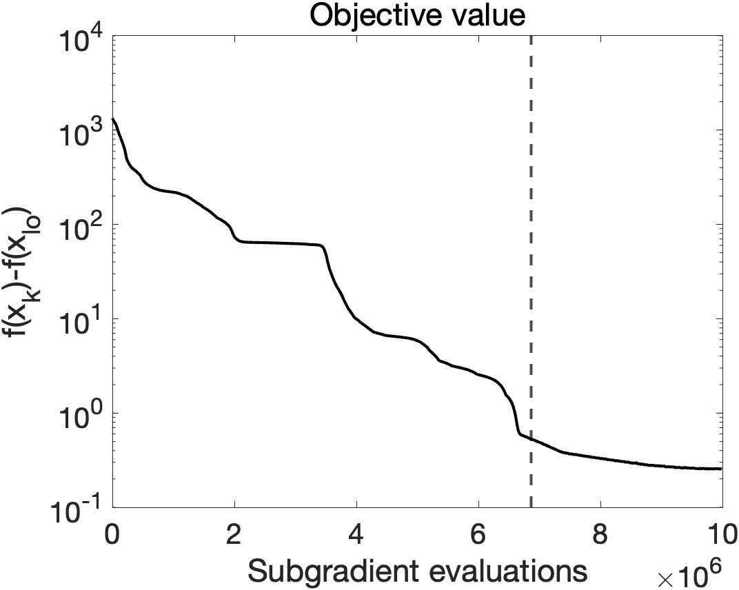
((a))

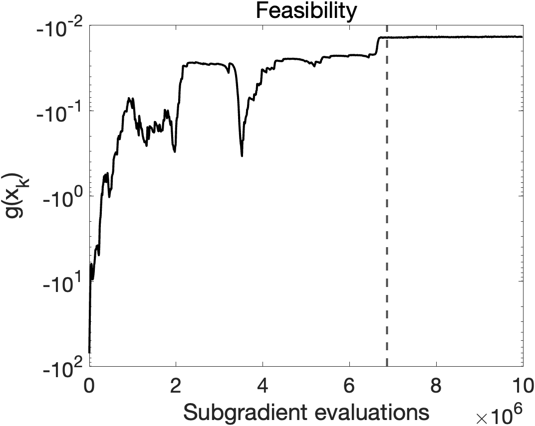
((b))

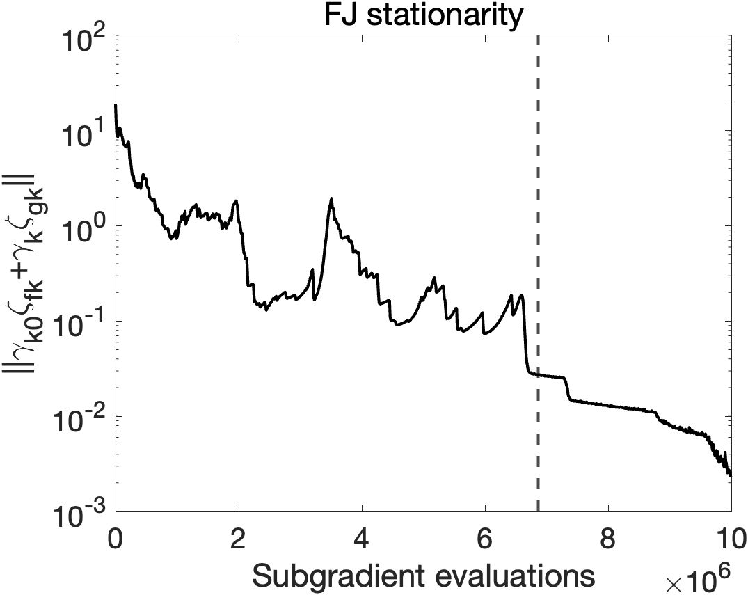
((c))

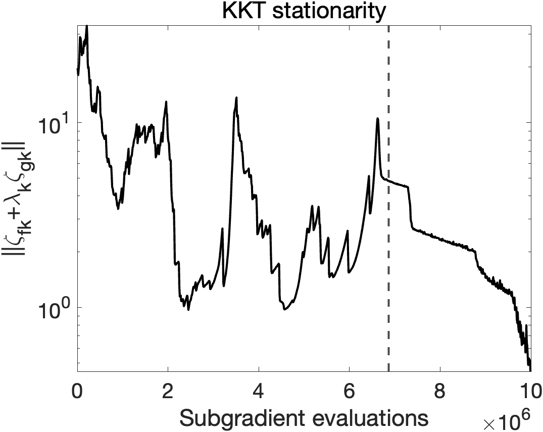
((d))

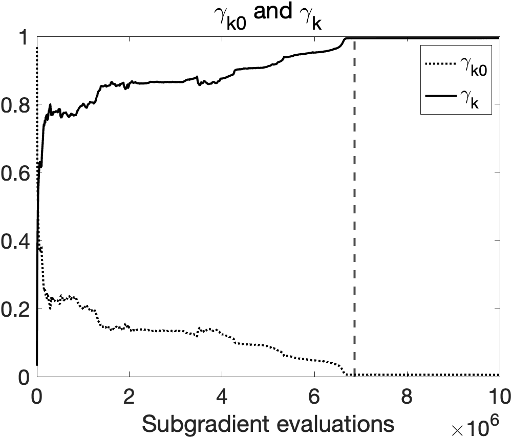
((e))

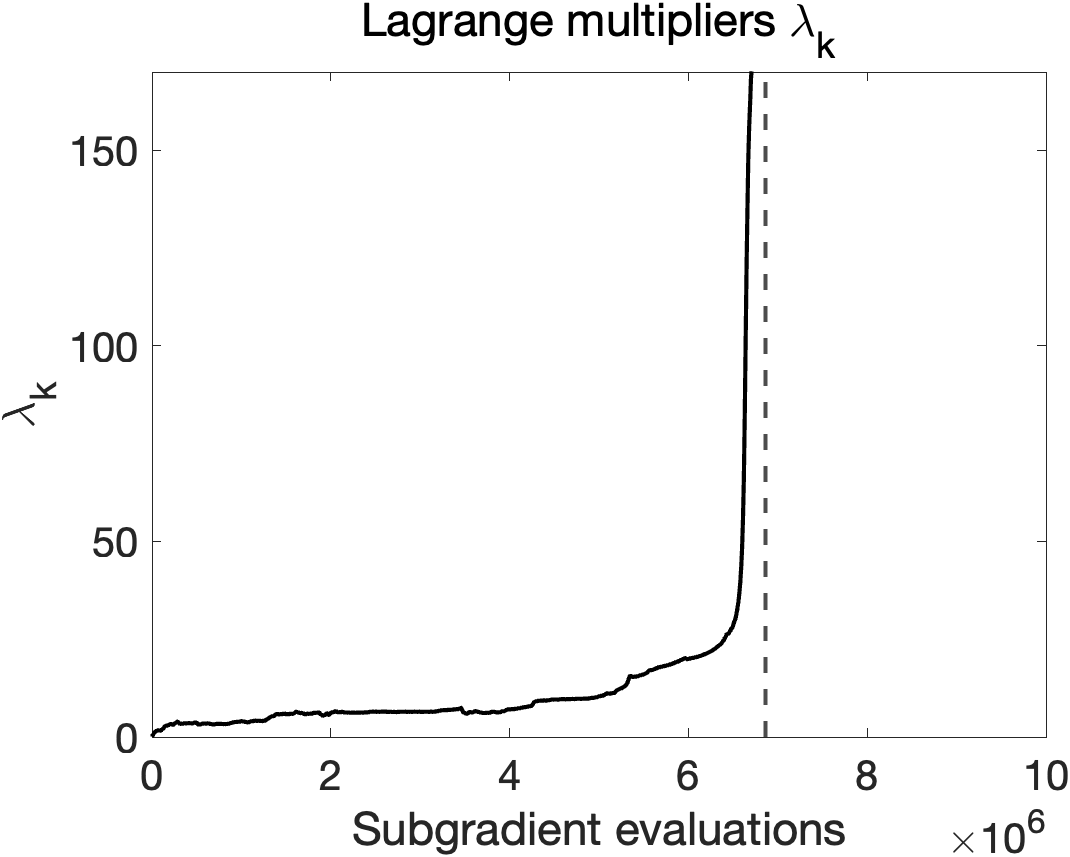
((f))

Figure 3: Finding FJ Stationarity: $K=10^{3},T=10^{4},p=90$. Dotted lines show where the stopping criteria applied. $x_{lo}$ is the stationary point near the final iterate.

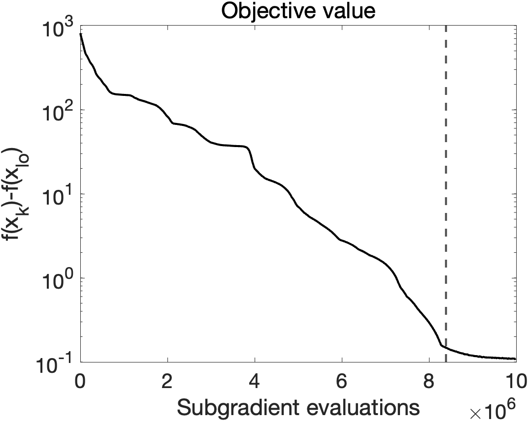
((a))

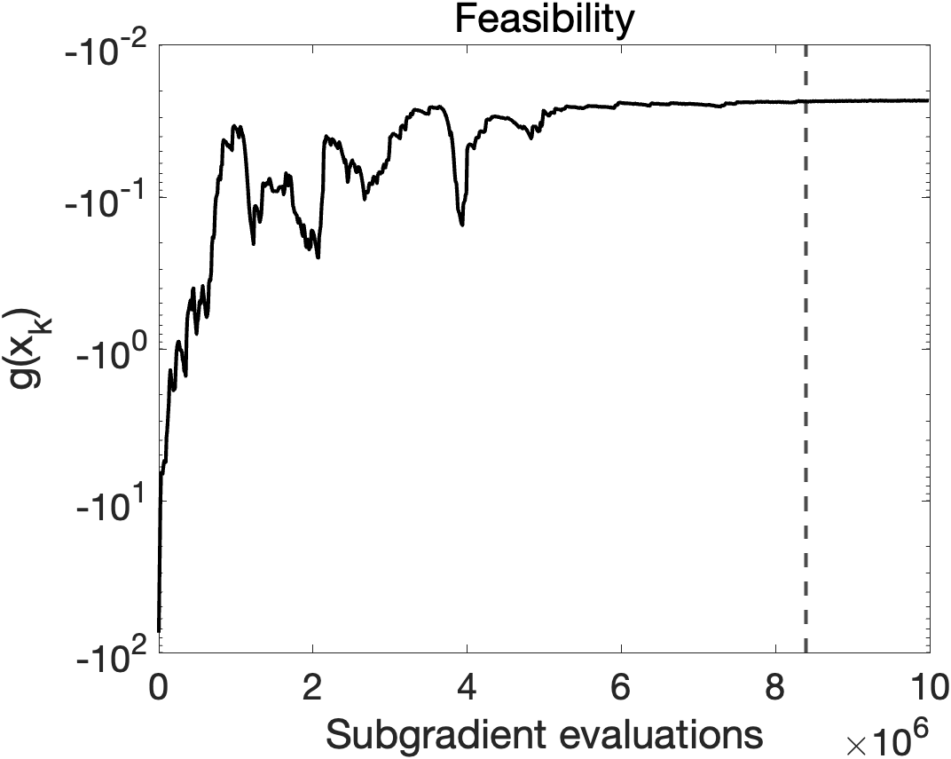
((b))

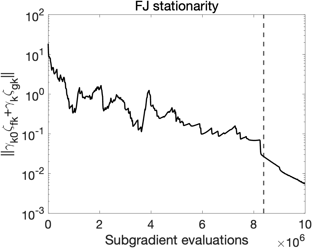
((c))

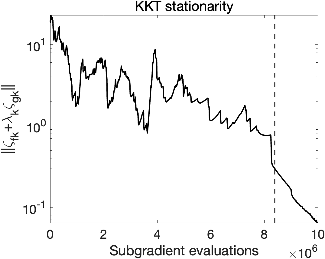
((d))

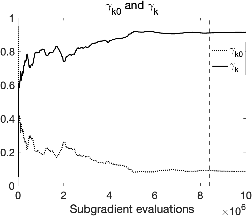
((e))

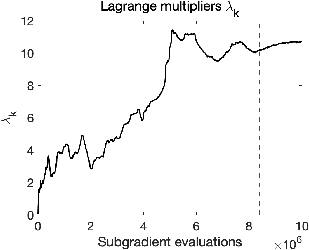
((f))

Figure 4: Finding Active KKT Stationarity: $K=10^{3},T=10^{4},p=91$. Dotted lines show where the stopping criteria applied. $x_{lo}$ is the stationary point near the final iterate.

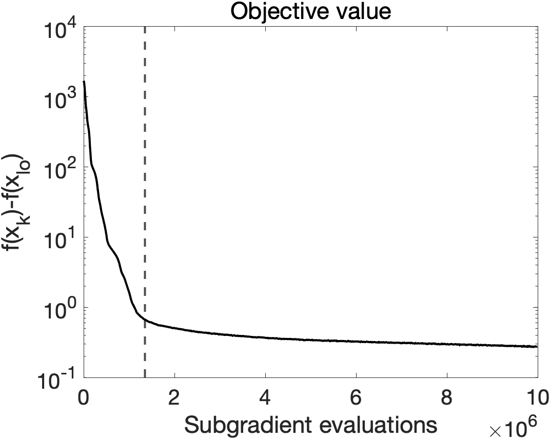
((a))

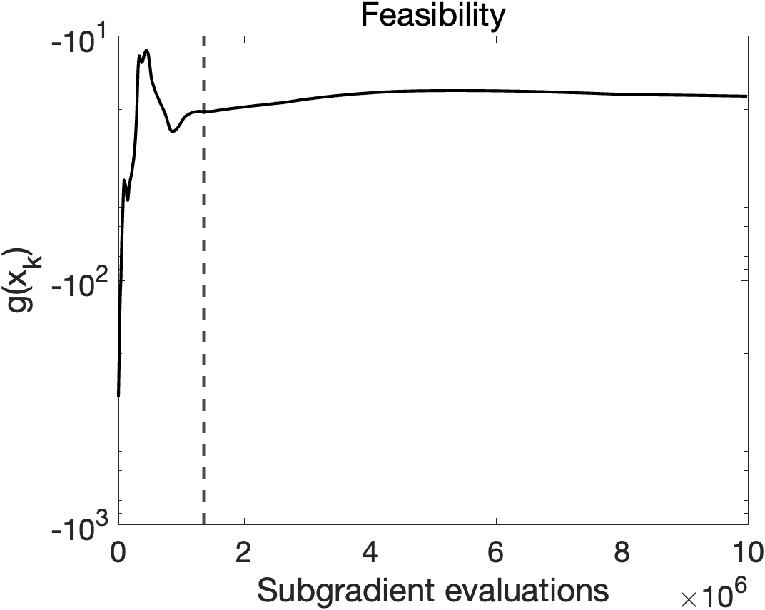
((b))

((c))

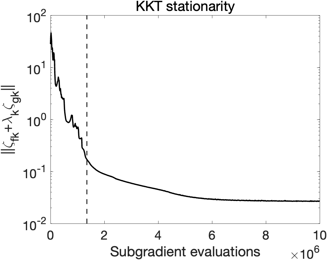
((d))

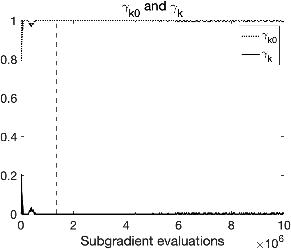
((e))

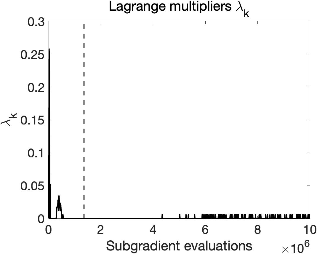
((f))

Figure 5: Finding Inactive KKT Stationarity: $K=10^{3},T=10^{4},p=320$. Dotted lines show where the stopping criteria applied. $x_{lo}$ is the stationary point near the final iterate.

$KT$		$p=90$		$p=91$		$p=320$
		$T=10^{3}$	$T=10^{4}$	$T=10^{3}$	$T=10^{4}$	$T=10^{3}$	$T=10^{4}$
$10^{5}$	median	$1.174$	$7.692$	$1.036$	$8.327$	$0.8860$	$16.11$
	mean	$1.239$	$7.992$	$1.060$	$8.272$	$0.9948$	$16.34$
	var.	$0.4265$	$1.329$	$0.1791$	$1.108$	$0.2032$	$11.49$
$10^{6}$	median	$0.03230$	$1.212$	$0.03370$	$1.032$	$0.06256$	$0.8309$
	mean	$0.04563$	$1.212$	$0.07497$	$1.181$	$0.07423$	$0.8853$
	var.	$2.587$e$-3$	$0.1937$	$0.03230$	$0.3225$	$1.487$e$-3$	$0.1453$
$10^{7}$	median	$0.03110$	$2.200$e$-3$	$0.03140$	$2.110$e$-3$	$0.06146$	$0.01910$
	mean	$0.03173$	$0.04273$	$0.03130$	$0.01644$	$0.06460$	$0.02941$
	var.	$2.545$e$-5$	$0.01340$	$2.062$e$-5$	$3.109$e$-3$	$2.926$e$-4$	$1.406$e$-3$

Table 1: FJ stationarity averaged over $50$ trails.

$KT$		$p=90$		$p=91$		$p=320$
		$T=10^{3}$	$T=10^{4}$	$T=10^{3}$	$T=10^{4}$	$T=10^{3}$	$T=10^{4}$
$10^{5}$	median	$6.904$	$22.94$	$6.515$	$24.44$	$0.9485$	$16.39$
	mean	$7.810$	$24.49$	$6.819$	$24.94$	$1.087$	$16.69$
	var.	$20.41$	$25.92$	$7.586$	$23.35$	$0.2966$	$15.54$
$10^{6}$	median	$0.2812$	$7.273$	$0.2987$	$6.599$	$0.07857$	$0.8309$
	mean	$0.3855$	$7.366$	$0.6012$	$7.364$	$0.08914$	$0.9364$
	var.	$0.1502$	$7.148$	$1.405$	$14.31$	$2.255$e$-3$	$0.1911$
$10^{7}$	median	$0.2740$	$0.01970$	$0.2900$	$0.01752$	$0.07256$	$0.0203$
	mean	$0.2829$	$0.5566$	$0.3146$	$0.1277$	$0.07728$	$0.03169$
	var.	$9.349$e$-3$	$1.777$	$0.01947$	$0.1580$	$4.596$e$-4$	$1.538$e$-3$

Table 2: KKT stationarity averaged over $50$ trails.

6 Conclusion and Future Directions

In this paper, we analyzed an inexact proximal point method using the switching subgradient method as an oracle for nonconvex nonsmooth functional constrained optimization. We derived new convergence rates towards FJ and KKT stationarity while guaranteeing feasibility for our solutions without any reliance on compactness or constraint qualification. The performance of our method for solving sparse phase retrieval problems is consistent with our theoretical expectations. The frequency of constraint qualification failures seen numerically here motivates further works analyzing the performance of nonconvex constrained optimization algorithms both in terms of KKT and FJ convergence. As additional future directions, stochastic versions of our method could likely be designed and analyzed, like those of [7, 21] from the unconstrained setting or those discussed at the end of Section 3.1. Further, convergence speedups in the presence of structures like local sharpness (see [50]), strong convexity, or smoothness at the stationary points may be possible.

Appendix A Deferred Proofs

A.1 Symmetric KKT Proof of Theorem 3.3

According to Lemma 3.5, our iterates are always feasible, that is $g(x_{k})\leq 0$, for the main problem (2.11) before $\hat{x}_{k+1}$ is an $\epsilon$-KKT point (which will imply $x_{k}$ is an $(\epsilon,\epsilon)$-KKT point). For each iteration $k$, let $\lambda_{k}$ denote the optimal Lagrange multiplier in (1.5) for the proximal subproblem (2.12). We denote the Lagrange function for each subproblem (2.12) as

$$L_{k}(x)=F_{k}(x)+\lambda_{k}G_{k}(x)=f(x)+\frac{\hat{\rho}}{2}\|x-x_{k}\|^{2}+\lambda_{k}(g(x)+\frac{\hat{\rho}}{2}\|x-x_{k}\|^{2})\ .$$ (A.1)

Without loss of generality, suppose $\lambda_{k}\geq 0$. According to KKT conditions (1.5), there exists $\hat{\zeta}_{Fk}\in\partial F_{k}(\hat{x}_{k+1})$ and $\hat{\zeta}_{Gk}\in\partial G_{k}(\hat{x}_{k+1})$ which satisfies

$$\hat{\zeta}_{Fk}+\lambda_{k}\hat{\zeta}_{Gk}\in-N_{X}(\hat{x}_{k+1})\ .$$ (A.2)

Since $L_{k}(x)$ is $(1+\lambda_{k})(\hat{\rho}-\rho)$-strongly convex, we have

$$F_{k}(x_{k})+\lambda_{k}G_{k}(x_{k})\geq F_{k}(\hat{x}_{k+1})+\lambda_{k}G_{k}(\hat{x}_{k+1})+(\hat{\zeta}_{Fk}+\lambda_{k}\hat{\zeta}_{Gk})^{T}(x_{k}-\hat{x}_{k+1})$$

$$+\frac{(1+\lambda_{k})(\hat{\rho}-\rho)}{2}\|\hat{x}_{k+1}-x_{k}\|^{2}\ .$$

According to KKT conditions (1.5), we also have $\lambda_{k}G_{k}(\hat{x}_{k+1})=0$. By (A.2) and since $x_{k}\in X$, we know $(\hat{\zeta}_{Fk}+\lambda_{k}\hat{\zeta}_{Gk})^{T}(x_{k}-\hat{x}_{k+1})\geq 0$. Since $g(x_{k})\leq 0$ from Lemma 3.5, the previous inequality becomes

$$f(x_{k})\geq F_{k}(\hat{x}_{k+1})+\frac{\hat{\rho}-\rho}{2}\|\hat{x}_{k+1}-x_{k}\|^{2}\ .$$

Since $x_{k+1}$ is a $(\tau,\tau)$-solution for problem (2.12), $F_{k}(x_{k+1})-F_{k}(\hat{x}_{k+1})\leq\tau$, then

$$f(x_{k}) \geq(f(x_{k+1})+\frac{\hat{\rho}}{2}\|x_{k+1}-x_{k}\|^{2}-\tau)+\frac{(1+\lambda_{k})(\hat{\rho}-\rho)}{2}\|\hat{x}_{k+1}-x_{k}\|^{2}$$

$$\geq f(x_{k+1})-\tau+\frac{(1+\lambda_{k})(\hat{\rho}-\rho)}{2}\|\hat{x}_{k+1}-x_{k}\|^{2}\ .$$

Thus we attain a lower bound for the descent of each step as

$$f(x_{k})-f(x_{k+1})\geq\frac{(1+\lambda_{k})(\hat{\rho}-\rho)}{2}\|\hat{x}_{k+1}-x_{k}\|^{2}-\tau\ .$$ (A.3)

Let $\hat{\zeta}_{fk}=\hat{\zeta}_{Fk}-\hat{\rho}(\hat{x}_{k+1}-x_{k})\in\partial f(\hat{x}_{k+1})$, $\hat{\zeta}_{gk}=\hat{\zeta}_{Gk}-\hat{\rho}(\hat{x}_{k+1}-x_{k})\in\partial g(\hat{x}_{k+1})$. According to (A.2) and Lemma 2.5, before $\hat{x}_{k+1}$ is an $\epsilon$-KKT point, there exists $\nu\in N_{X}(\hat{x}_{k+1})$ which satisfies:

$$(\hat{\zeta}_{fk}+\hat{\rho}(\hat{x}_{k+1}-x_{k}))+\lambda_{k}(\hat{\zeta}_{gk}+\hat{\rho}(\hat{x}_{k+1}-x_{k}))+\nu=0\ ,$$

$$\|\hat{\zeta}_{fk}+\lambda_{k}\hat{\zeta}_{gk}+\nu\|>\epsilon\ .$$

As a result, $\|\hat{x}_{k+1}-x_{k}\|>\frac{\epsilon}{(1+\lambda_{k})\hat{\rho}}$. Thus, before $\hat{x}_{k+1}$ is an $\epsilon$-KKT point, our choice of $\tau$ ensures

$$f(x_{k})-f(x_{k+1}) \geq\frac{(1+\lambda_{k})(\hat{\rho}-\rho)}{2}\|\hat{x}_{k+1}-x_{k}\|^{2}-\tau$$

$$>\frac{(1+\lambda_{k})(\hat{\rho}-\rho)}{2}\frac{\epsilon^{2}}{(1+\lambda_{k})^{2}\hat{\rho}^{2}}-\frac{(\hat{\rho}-\rho)\epsilon^{2}}{4(1+B)^{2}\hat{\rho}(2\hat{\rho}-\rho)}$$

$$>\frac{(\hat{\rho}-\rho)\epsilon^{2}}{2(1+\lambda_{k})\hat{\rho}^{2}}-\frac{(\hat{\rho}-\rho)\epsilon^{2}}{4(1+B)\hat{\rho}(2\hat{\rho}-\rho)}$$

$$\geq\frac{(\hat{\rho}-\rho)\epsilon^{2}}{2(1+B)\hat{\rho}^{2}}-\frac{(\hat{\rho}-\rho)\epsilon^{2}}{4(1+B)\hat{\rho}^{2}}$$

$$=\frac{(\hat{\rho}-\rho)\epsilon^{2}}{4(1+B)\hat{\rho}^{2}}\ .$$

By Assumption B, we could give an upper bound for the number of total iterations $K$ as

$$K<\frac{4(1+B)\hat{\rho}^{2}(f(x_{0})-f_{lb})}{(\hat{\rho}-\rho)\epsilon^{2}}\ .$$

Consequently, Algorithm 2 (which uses Algorithm 1 for $T$ steps as an oracle each iteration) will identify an $(\epsilon,\epsilon)$-KKT point using at most $KT=O(1/\epsilon^{4})$ total subgradient evaluations of either the objective or constraints.

A.2 Symmetric KKT Case of Lemma 2.5’s Proof

Given constraint qualification, necessarily, the KKT conditions are satisfied for the proximal subproblem (2.12) by some $\lambda_{k}\geq 0$, $\hat{\zeta}_{Fk}\in\partial F_{k}(\hat{x}_{k+1})$ and $\hat{\zeta}_{Gk}\in\partial G_{k}(\hat{x}_{k+1})$. By the sum rule, let $\hat{\zeta}_{fk}=\hat{\zeta}_{Fk}-\hat{\rho}(\hat{x}_{k+1}-x_{k})\in\partial f(\hat{x}_{k+1})$ and $\hat{\zeta}_{gk}=\hat{\zeta}_{Gk}-\hat{\rho}(\hat{x}_{k+1}-x_{k})\in\partial g(\hat{x}_{k+1})$. The KKT conditions for the proximal subproblem ensure some $\nu\in N_{X}(\hat{x}_{k+1})$ has

$$\hat{\zeta}_{fk}+\hat{\rho}(\hat{x}_{k+1}-x_{k})+\lambda_{k}(\hat{\zeta}_{gk}+\hat{\rho}(\hat{x}_{k+1}-x_{k}))=-\nu\ .$$

When $\|\hat{x}_{k+1}-x_{k}\|\leq\frac{\epsilon}{\hat{\rho}(1+\lambda_{k})}$, it follows that $\|\hat{\zeta}_{fk}+\lambda_{k}\hat{\zeta}_{gk}+\nu\|=\hat{\rho}(1+\lambda_{k})\|\hat{x}_{k+1}-x_{k}\|\leq\epsilon$, establishing the first approximate KKT condition (2.7).

We verify the second approximate KKT condition (2.8) in two cases: When $\lambda_{k}=0$, trivially $|\lambda_{k}g(\hat{x}_{k+1})|=0$. When $\lambda_{k}$ is positive, the KKT conditions for the proximal subproblem require $G_{k}(\hat{x}_{k+1})=0$. Hence $0\geq g(\hat{x}_{k+1})=-\frac{\hat{\rho}}{2}\|\hat{x}_{k+1}-x_{k}\|^{2}\geq-\frac{\epsilon^{2}}{2\hat{\rho}(1+\lambda_{k})^{2}}$ . Therefore

$$|\lambda_{k}g(\hat{x}_{k+1})|\leq\frac{\epsilon^{2}\lambda_{k}}{2\hat{\rho}(1+\lambda_{k})^{2}}\leq\frac{\epsilon^{2}}{2\hat{\rho}}<\epsilon^{2}\ .$$

A.3 Symmetric KKT Case of Lemma 3.5’s Proof

Assume $G_{k}(x_{k})=g(x_{k})\leq 0$. Necessarily, there exists an optimal dual variable for the subproblem $\lambda_{k}$. For the Lagrange function $L_{k}(x)=F_{k}(x)+\lambda_{k}G_{k}(x)$, which $\hat{x}_{k+1}$ minimizes, its $(1+\lambda_{k})(\hat{\rho}-\rho)$-strong convexity ensures

$$F_{k}(x_{k+1})+\lambda_{k}G_{k}(x_{k+1})\geq F_{k}(\hat{x}_{k+1})+\lambda_{k}G_{k}(\hat{x}_{k+1})+(\hat{\zeta}_{Fk}+\lambda_{k}\hat{\zeta}_{Gk})^{T}(x_{k+1}-\hat{x}_{k+1})$$

$$+\frac{(1+\lambda_{k})(\hat{\rho}-\rho)}{2}\|x_{k+1}-\hat{x}_{k+1}\|^{2}\ .$$

Note the KKT conditions ensure that $\lambda_{k}G_{k}(\hat{x}_{k+1})=0$ and that $\hat{\zeta}_{Fk}+\lambda_{k}\hat{\zeta}_{Gk}\in-N_{X}(\hat{x}_{k+1})$, from which one can conclude $x_{k+1}\in X$ must have $(\zeta_{Fk}+\lambda_{k}\zeta_{Gk})^{T}(x_{k+1}-\hat{x}_{k+1})\geq 0$. Then the above inequality simplifies to

$$F_{k}(x_{k+1})-F_{k}(\hat{x}_{k+1})+\lambda_{k}G_{k}(x_{k+1})\geq\frac{(1+\lambda_{k})(\hat{\rho}-\rho)}{2}\|x_{k+1}-\hat{x}_{k+1}\|^{2}\ .$$

The proposed value of $T$ ensures $x_{k+1}$ is a $(\tau,\tau)$-optimal solution for the subproblem (2.12), i.e., $F_{k}(x_{k+1})-F_{k}(\hat{x}_{k+1})\leq\tau$ and $G_{k}(x_{k+1})\leq\tau$. Hence

$$\|\hat{x}_{k+1}-x_{k+1}\| \leq\sqrt{\frac{2\tau}{\hat{\rho}-\rho}}\ .$$

Let $\hat{\zeta}_{fk}=\hat{\zeta}_{Fk}-\hat{\rho}(\hat{x}_{k+1}-x_{k})\in\partial f(\hat{x}_{k+1})$, $\hat{\zeta}_{gk}=\hat{\zeta}_{Gk}-\hat{\rho}(\hat{x}_{k+1}-x_{k})\in\partial g(\hat{x}_{k+1})$. There must exists $\nu\in N_{X}(\hat{x}_{k+1})$ such that $\hat{\zeta}_{fk}+\hat{\rho}(\hat{x}_{k+1}-x_{k})+\lambda_{k}(\hat{\zeta}_{gk}+\hat{\rho}(\hat{x}_{k+1}-x_{k}))+\nu=0$. However, assuming $\hat{x}_{k+1}$ is not an $\epsilon$-KKT point, $\|\gamma_{k0}\hat{\zeta}_{fk}+\gamma_{k}\hat{\zeta}_{gk}+\nu\|>\epsilon$, which implies $\|\hat{x}_{k+1}-x_{k}\|>\frac{\epsilon}{(1+B)\hat{\rho}}$. Thus

$$\|x_{k+1}-x_{k}\|^{2}\geq\frac{1}{2}\|\hat{x}_{k+1}-x_{k}\|^{2}-\|\hat{x}_{k+1}-x_{k+1}\|^{2}>\frac{\epsilon^{2}}{2(1+B)^{2}\hat{\rho}^{2}}-\frac{2\tau}{\hat{\rho}-\rho}\ .$$

By our selection of $\tau=\frac{(\hat{\rho}-\rho)\epsilon^{2}}{4(1+B)^{2}\hat{\rho}(2\hat{\rho}-\rho)}$ as in (3.4), every iteration prior to finding an $\epsilon$-KKT point must have

$$\|x_{k+1}-x_{k}\|^{2}>\frac{(\hat{\rho}-\rho)\epsilon^{2}}{2(1+B)^{2}\hat{\rho}^{2}(2\hat{\rho}-\rho)}\ .$$ (A.4)

Therefore $g(x_{k+1})\leq 0$ is inductively ensured if $g(x_{k})\leq 0$ and $\hat{x}_{k+1}$ is not an $\epsilon$-KKT point as

$$g(x_{k+1})=G(x_{k+1})-\frac{\hat{\rho}}{2}\|x_{k+1}-x_{k}\|^{2}\leq\tau-\frac{\hat{\rho}}{2}\frac{(\hat{\rho}-\rho)\epsilon^{2}}{2(1+B)^{2}\hat{\rho}^{2}(2\hat{\rho}-\rho)}=0\ .$$

References

- [1] Runchao Ma, Qihang Lin, and Tianbao Yang. Quadratically regularized subgradient methods for weakly convex optimization with weakly convex constraints. In International Conference on Machine Learning, pages 6554–6564. PMLR, 2020.
- [2] Digvijay Boob, Qi Deng, and Guanghui Lan. Stochastic first-order methods for convex and nonconvex functional constrained optimization. Mathematical Programming, pages 1–65, 2022.
- [3] Damek Davis, Dmitriy Drusvyatskiy, and Courtney Paquette. The nonsmooth landscape of phase retrieval. IMA Journal of Numerical Analysis, 40(4):2652–2695, 2020.
- [4] John C Duchi and Feng Ruan. Solving (most) of a set of quadratic equalities: Composite optimization for robust phase retrieval. Information and Inference: A Journal of the IMA, 8(3):471–529, 2019.
- [5] Vasileios Charisopoulos, Damek Davis, Mateo Díaz, and Dmitriy Drusvyatskiy. Composite optimization for robust rank one bilinear sensing. Information and Inference: A Journal of the IMA, 10(2):333–396, 2021.
- [6] Yuxin Chen, Yuejie Chi, and Andrea J Goldsmith. Exact and stable covariance estimation from quadratic sampling via convex programming. IEEE Transactions on Information Theory, 61(7):4034–4059, 2015.
- [7] Damek Davis and Dmitriy Drusvyatskiy. Stochastic model-based minimization of weakly convex functions. SIAM Journal on Optimization, 29(1):207–239, 2019.
- [8] Anestis Antoniadis. Wavelets in statistics: a review. Journal of the Italian Statistical Society, 6(2):97–130, 1997.
- [9] Jianqing Fan and Runze Li. Variable selection via nonconcave penalized likelihood and its oracle properties. Journal of the American statistical Association, 96(456):1348–1360, 2001.
- [10] Yongdai Kim, Hosik Choi, and Hee-Seok Oh. Smoothly clipped absolute deviation on high dimensions. Journal of the American Statistical Association, 103(484):1665–1673, 2008.
- [11] Jianqing Fan, Yang Feng, and Yichao Wu. Network exploration via the adaptive lasso and scad penalties. The annals of applied statistics, 3(2):521, 2009.
- [12] Huiliang Xie and Jian Huang. Scad-penalized regression in high-dimensional partially linear models. The Annals of Statistics, 37(2):673–696, 2009.
- [13] Gilles Gasso, Alain Rakotomamonjy, and Stéphane Canu. Recovering sparse signals with a certain family of nonconvex penalties and dc programming. IEEE Transactions on Signal Processing, 57(12):4686–4698, 2009.
- [14] Jinshan Zeng, Wotao Yin, and Ding-Xuan Zhou. Moreau envelope augmented lagrangian method for nonconvex optimization with linear constraints. Journal of Scientific Computing, 91(2):1–36, 2022.
- [15] Jason Weston and Chris Watkins. Multi-class support vector machines. Technical report, Citeseer, 1998.
- [16] Ye Tian and Yang Feng. Neyman-pearson multi-class classification via cost-sensitive learning. arXiv preprint arXiv:2111.04597, 2021.
- [17] Warren Hare and Claudia Sagastizábal. Computing proximal points of nonconvex functions. Mathematical Programming, 116(1):221–258, 2009.
- [18] Warren Hare and Claudia Sagastizábal. A redistributed proximal bundle method for nonconvex optimization. SIAM Journal on Optimization, 20(5):2442–2473, 2010.
- [19] Saverio Salzo and Silvia Villa. Inexact and accelerated proximal point algorithms. Journal of Convex analysis, 19(4):1167–1192, 2012.
- [20] Courtney Paquette, Hongzhou Lin, Dmitriy Drusvyatskiy, Julien Mairal, and Zaid Harchaoui. Catalyst for gradient-based nonconvex optimization. In International Conference on Artificial Intelligence and Statistics, pages 613–622. PMLR, 2018.
- [21] Damek Davis and Benjamin Grimmer. Proximally guided stochastic subgradient method for nonsmooth, nonconvex problems. SIAM Journal on Optimization, 29(3):1908–1930, 2019.
- [22] Fritz John. Extremum problems with inequalities as subsidiary conditions. In Traces and emergence of nonlinear programming, pages 197–215. Springer, 2014.
- [23] Olvi L Mangasarian and Stan Fromovitz. The fritz john necessary optimality conditions in the presence of equality and inequality constraints. Journal of Mathematical Analysis and applications, 17(1):37–47, 1967.
- [24] Frank Allgöwer and Alex Zheng. Nonlinear model predictive control, volume 26. Birkhäuser, 2012.
- [25] Zhengshi Yu, Pingyuan Cui, and John L Crassidis. Design and optimization of navigation and guidance techniques for mars pinpoint landing: Review and prospect. Progress in Aerospace Sciences, 94:82–94, 2017.
- [26] Fei Wen, Ling Pei, Yuan Yang, Wenxian Yu, and Peilin Liu. Efficient and robust recovery of sparse signal and image using generalized nonconvex regularization. IEEE Transactions on Computational Imaging, 3(4):566–579, 2017.
- [27] Fei Wen, Lei Chu, Peilin Liu, and Robert C Qiu. A survey on nonconvex regularization-based sparse and low-rank recovery in signal processing, statistics, and machine learning. IEEE Access, 6:69883–69906, 2018.
- [28] Hui Zhang, Shou-Jiang Li, Hai Zhang, Zi-Yi Yang, Yan-Qiong Ren, Liang-Yong Xia, and Yong Liang. Meta-analysis based on nonconvex regularization. Scientific reports, 10(1):1–16, 2020.
- [29] Konstantin Pieper and Armenak Petrosyan. Nonconvex regularization for sparse neural networks. Applied and Computational Harmonic Analysis, 2022.
- [30] Aleksandr Y Aravkin, James V Burke, Dmitry Drusvyatskiy, Michael P Friedlander, and Scott Roy. Level-set methods for convex optimization. Mathematical Programming, 174(1):359–390, 2019.
- [31] Qihang Lin, Selvaprabu Nadarajah, and Negar Soheili. A level-set method for convex optimization with a feasible solution path. SIAM Journal on Optimization, 28(4):3290–3311, 2018.
- [32] Boris Polyak. A general method for solving extremum problems. Soviet Mathematics. Doklady, 8, 01 1967.
- [33] Anastasia Bayandina, Pavel Dvurechensky, Alexander Gasnikov, Fedor Stonyakin, and Alexander Titov. Mirror descent and convex optimization problems with non-smooth inequality constraints. In Large-scale and distributed optimization, pages 181–213. Springer, 2018.
- [34] Guanghui Lan and Zhiqiang Zhou. Algorithms for stochastic optimization with function or expectation constraints. Computational Optimization and Applications, 76(2):461–498, 2020.
- [35] Ernesto G Birgin, JL Gardenghi, José Mario Martínez, Sandra A Santos, and Ph L Toint. Evaluation complexity for nonlinear constrained optimization using unscaled kkt conditions and high-order models. SIAM Journal on Optimization, 26(2):951–967, 2016.
- [36] Oliver Hinder and Yinyu Ye. Worst-case iteration bounds for log barrier methods for problems with nonconvex constraints. arXiv preprint arXiv:1807.00404, 2018.
- [37] Coralia Cartis, Nicholas IM Gould, and Philippe L Toint. On the evaluation complexity of composite function minimization with applications to nonconvex nonlinear programming. SIAM Journal on Optimization, 21(4):1721–1739, 2011.
- [38] Coralia Cartis, Nicholas IM Gould, and Philippe L Toint. On the evaluation complexity of cubic regularization methods for potentially rank-deficient nonlinear least-squares problems and its relevance to constrained nonlinear optimization. SIAM Journal on Optimization, 23(3):1553–1574, 2013.
- [39] Coralia Cartis, Nicholas IM Gould, and Philippe L Toint. On the complexity of finding first-order critical points in constrained nonlinear optimization. Mathematical Programming, 144(1):93–106, 2014.
- [40] Coralia Cartis, Nick Gould, and Philippe L Toint. Strong evaluation complexity bounds for arbitrary-order optimization of nonconvex nonsmooth composite functions. arXiv preprint arXiv:2001.10802, 2020.
- [41] Jorge Nocedal and Stephen J. Wright. Sequential Quadratic Programming, pages 529–562. Springer New York, New York, NY, 2006.
- [42] Coralia Cartis, Nicholas I. M. Gould, and Philippe L. Toint. On the evaluation complexity of constrained nonlinear least-squares and general constrained nonlinear optimization using second-order methods. SIAM J. Numer. Anal., 53(2):836–851, jan 2015.
- [43] Francisco Facchinei, Vyacheslav Kungurtsev, Lorenzo Lampariello, and Gesualdo Scutari. Ghost penalties in nonconvex constrained optimization: Diminishing stepsizes and iteration complexity. Mathematics of Operations Research, 46(2):595–627, 2021.
- [44] Xiao Wang, Shiqian Ma, and Ya-Xiang Yuan. Penalty methods with stochastic approximation for stochastic nonlinear programming. Mathematics of Computation, 86(306):1793–1820, 2017.
- [45] Benjamin Grimmer. Radial Duality Part I: Foundations, 2021.
- [46] Benjamin Grimmer. Radial Duality Part II: Applications and Algorithms, 2021.
- [47] Benjamin Grimmer. Convergence rates for deterministic and stochastic subgradient methods without lipschitz continuity. SIAM Journal on Optimization, 29(2):1350–1365, 2019.
- [48] Robert Mansel Gower, Nicolas Loizou, Xun Qian, Alibek Sailanbayev, Egor Shulgin, and Peter Richtárik. Sgd: General analysis and improved rates. In International Conference on Machine Learning, pages 5200–5209. PMLR, 2019.
- [49] Simon Lacoste-Julien, Mark Schmidt, and Francis Bach. A simpler approach to obtaining an o(1/t) convergence rate for the projected stochastic subgradient method, 2012.
- [50] Damek Davis, Dmitriy Drusvyatskiy, Kellie J MacPhee, and Courtney Paquette. Subgradient methods for sharp weakly convex functions. Journal of Optimization Theory and Applications, 179(3):962–982, 2018.