3D-LDM: Neural Implicit 3D Shape Generation with Latent Diffusion Models

Abstract

Diffusion models have shown great promise for image generation, beating GANs in terms of generation diversity, with comparable image quality. However, their application to 3D shapes has been limited to point or voxel representations that can in practice not accurately represent a 3D surface. We propose a diffusion model for neural implicit representations of 3D shapes that operates in the latent space of an auto-decoder. This allows us to generate diverse and high quality 3D surfaces. We additionally show that we can condition our model on images or text to enable image-to-3D generation and text-to-3D generation using CLIP embeddings. Furthermore, adding noise to the latent codes of existing shapes allows us to explore shape variations.

1 Introduction

Denoising Diffusion Probabilistic Models (DDPMs) [21] are an emerging paradigm for generating novel high-quality and diverse content, revolutionizing workflows to create images [40, 46, 50, 70], audio [29, 10], and video [54, 20]. DDPMs provide several advantages over other generative models like GANs: they tend to improve coverage of the data distribution, tend to be more stable at training time, and facilitate applications like inpainting. Most DDPMs work on 2D images, leveraging their canonical representation as pixel grids. Only recently have researchers started adopting them to generate 3D content, which has a less standardized representation, ranging from voxels, point clouds, meshes, and implicit functions. This wide variety of possible representation makes an application of DDPMs to 3D shapes less straight-forward.

A large body of prior work on generating 3D shapes focuses on voxels [5, 66] and point clouds [30, 6, 67, 33, 72, 71]. However, neither format is ideal for downstream creative needs: voxels are computationally and memory intensive and thus difficult to scale to high resolution; point clouds are light-weight and easy to process, but require a lossy post-processing step to obtain surfaces, which are required for some down-stream applications like rendering or modelling. On the contrary, neural implicit functions [42, 38] do provide an accurate and efficient representation for surfaces. However, it is not immediately clear how we can generate such a representation with a diffusion model.

In this work, we propose 3D-LDM, a novel method for generating neural implicit representations of 3D shapes. We have been inspired by Latent Diffusion Models (LDMs) for 2D images [48]. Our key insight is that we can generate neural implicit representations of 3D shapes (Signed Distance Functions - SDFs [69, 47, 17]) by applying a simple diffusion model to the latent space of an auto-decoder for 3D shapes like DeepSDF [42], therefore bypassing the need to directly operate on continuous surfaces. We show that this approach is significantly better than directly sampling from the latent space of the autodecoder and outperforms the previous state-of-the-art in unconditional 3D shape generation. Unlike existing diffusion-based approaches, we can generate neural implicit shape representations that allows us to extract high-quality surfaces. Compared to existing GAN-based models for generating neural implicit representations [64, 31, 8], our diffusion-based approach achieves better data coverage and sample quality. Additionally, 3D-LDM can easily be conditioned on context variables such as CLIP embeddings or images to enable both text-to-3D and image-to-3D generation. We also show that 3D-LDM can create variations of existing shapes by adding small amounts of noise, enabling a form of guided shape exploration.

In summary, our contribution is threefold:

• We propose a latent diffusion model that generates 3D implicit functions.

• We demonstrate text- and image-conditioned generation.

• We propose guided shape exploration based on adding noise to generated or existing shapes.

2 Related Work

3D-LDM is a diffusion model for 3D shapes represented as neural implicit functions, thus we review the work on 3D shape generation, 3D diffusion models, and methods that generate neural implicit functions, also in a conditional setting.

3D deep generative models. GAN [1, 65, 16, 61, 53], Flow [67, 27, 28], Score-Matching [7], Autoregressive [59], Diffusion (DDPM) [33, 72] or Energy (EBMs) [35] aim to approximate the distribution $p_{\theta}$ of a dataset $\mathcal{D}$. Thus, sampling from this data distribution allows the generation of novel shapes. However, since no ground truth for the new shapes is available, it requires likelihood-based evaluation metrics [1], to better evaluate if the model is overfitting on that distribution or generating novel shapes.

3D diffusion models. DDPMs [21, 56, 57, 68], cover the current state-of-the-art in image generation tasks outperforming GANs [13]. These models belong to latent variable models that have been inspired by non-equilibrium in thermodynamics literature and seek to gradually inject noise to the data distribution until an isotropic Gaussian is reached [56, 2]. This paradigm has been successfully adopted in 3D domains [33, 72, 71, 16, 24], showing promising results for diverse and high-quality shape generation. However, most works consider point clouds, or voxels, as the 3D representation, which are inherently limiting for graphics-based applications such as animation. We instead consider implicit functions, i.e. continuous surfaces, as our data representation which is more ideal for graphics-based rendering. Furthermore, previous diffusion models have been mainly applied to the data distribution, while we consider modeling latent distribution, echoing the recent success demonstrated by [57, 71].

3D shape generation via implicit function. Neural implicit representations seek to parameterize surfaces with continuous functions, making them simple while preserving fine-grained details. Prior works [11, 36, 42, 17, 39] adopted implicit representations for reconstruction tasks and some recent works such as Spaghetti [19] and Neural Wavelet [24] started using it for generation tasks. Neural Wavelet [24] and Spaghetti [19] respectively focused on multi-scale and part-aware implicit surface generation, which overcomes previous limitations of unstructured point cloud [72, 33] and voxel-based methods [72]. Similarly, LION [71] overcomes the above-mentioned limitations via a differentiable Shape as Point (SAP) module [43]. Unfortunately, LION does not leverage SAP’s differentiable property within its network, adding an extra computational burden.

Conditional Generation. Generative models can be conditioned on additional contexts such as classes [13, 23], latent space [41], noise signal [55] or others [22, 23]. Conditioning allows for more control in the generative process. While previous approaches focused on 2D images, few examples successfully translated to 3D objects or scenes. PVD [72] conditions on a depth-map. In concurrent work, GAUDI [4] uses sparse images to generate novel 3D scenes, disentangling camera poses from scene representation. However, novel 3D scene generation is not demonstrated conclusively. Our method can be conditioned on a CLIP-embedding that can be obtained from text or images, similar to previous work on 2D image generation [52, 63, 26, 37, 25, 44].

3 Method

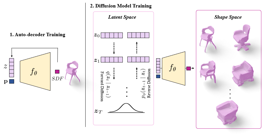
Figure 2: Overview of our architecture. In the first Stage, an auto-decoder is pre-trained to represent a set of 3D shapes; in the second stage, a diffusion model is trained on the latent space of the auto-decoder. At generation time, the diffusion model creates latent shape codes that are decoded into neural implicit 3D shapes by the pre-trained auto-decoder.

3D-LDM is a diffusion model for 3D shapes that is applied to a probabilistic auto-decoder [60, 42]. We train it following a two-stage process. First, a latent space for a dataset of SDF-based shapes is constructed by training an auto-decoder that accepts a latent vector directly as an input. Second, the auto-decoder is frozen and a DDPM [21] is trained on the latent representation of the 3D shapes, effectively decoupling the 3D shape representation from the output representation used by the DDPM. This allows us to use the DDPM to generate neural implicit 3D shapes when using an appropriate auto-decoder. An overview is shown in Figure 2. In the following sections, we describe the two stages in detail.

3.1 Auto-decoder for Neural Implicit 3D Shapes

Neural implicit shape representation.

In an implicit representation, the surface $S$ of a 3D shape is represented by the $0$-level set of a continuous function $f$ defined over the 3D space:

$$S\coloneqq\{\mathbf{p}\ |\ f(\mathbf{p})=0\},$$ (1)

with $\mathbf{p}\in\mathbb{R}^{3}$. We use the Signed Distance Function (SDF) as function $f$, which is defined as the signed distance to a (watertight) surface $S$; positive outside and negative inside.

In our approach, we work with neural implicit representations, where the function $f$ is efficiently represented by a neural network $f_{\theta}$:

$$S\coloneqq\{\mathbf{p}\ |\ f_{\theta}(\mathbf{p})=0\},$$ (2)

with network parameters $\theta$. A set of shapes $\mathcal{S}$ can be represented with $f_{\theta}$ by additionally conditioning $f_{\theta}$ on latent representations ${\bm{z}}_{i}$ of the shapes:

$$S_{i}\coloneqq\{\mathbf{p}\ |\ f_{\theta}(\mathbf{p},{\bm{z}}_{i})=0\},$$ (3)

with $S_{i}\in\mathcal{S}$.

We adopt the architecture proposed in DeepSDF [42] for $f_{\theta}$, with a few changes that empirically improve the quality of the generated shape distribution. We refer readers to supplementary material for further details.

Training setup.

DeepSDF [42] has shown that $f_{\theta}$ can be trained efficiently in an encoder-less setup, called an auto-decoder, where each shape $S_{i}$ is explicitly associated with a latent vector ${\bm{z}}_{i}$, by storing a list of latent vectors $Z=({\bm{z}}_{1},\dots,{\bm{z}}_{N})$, one for each of the $N$ shapes in $\mathcal{S}$. At training time, we optimize both $Z$ and $\theta$ to minimize the reconstruction error:

$$\operatorname*{arg\,min}_{\theta,Z}\sum_{i=1}^{N}\mathcal{L}_{\text{recon}}({\bm{z}}_{i},\text{SDF}_{i})+\frac{1}{\lambda^{2}}\mathcal{L}_{\text{reg}}({\bm{z}}_{i}),\text{ with}$$ (4)

$$\mathcal{L}_{\text{recon}}\coloneqq\mathbb{E}_{\mathbf{p}\sim\mathcal{P}}\left[\|f_{\theta}(\mathbf{p},{\bm{z}}_{i})-\text{SDF}_{i}(\mathbf{p})\|_{1}\right],\text{ and}$$

$$\mathcal{L}_{\text{reg}}\coloneqq\|{\bm{z}}_{i}\|_{2}^{2}.$$ (5)

$\text{SDF}_{i}$ is the ground truth signed distance function for shape $S_{i}$, and $\mathcal{P}$ is the distribution of training sample points, which are either sampled uniformly in the shape bounding box, or close to the shape surface. The term $\mathcal{L}_{\text{reg}}$ regularizes the magnitude of the latent vectors to improve their layout in the latent space and make them easier to generate in our second stage; $\lambda$ is the regularization factor. Similar to DeepSDF, we clamp the predicted and ground truth signed distances to an interval $[-\delta,\delta]$, as predicting accurate distances far away from the surface is not necessary. For further details about the training setup, we refer the reader to Section B in the supplementary material.

Note that we cannot directly sample novel shapes from the latent space of the auto-decoder $f_{\theta}$, since the probability distribution of the latent data samples ${\bm{z}}_{i}$ is unknown. Instead, we train a diffusion model on the samples ${\bm{z}}_{i}$.

3.2 Latent Diffusion Model

We base our diffusion model on DDPM [21]. Diffusion models consist of two processes, a forward process and a reverse process.

Forward process.

The forward process iteratively adds Gaussian noise to the shape latents in multiple steps, such that their distribution is indistinguishable from the standard normal distribution after $T$ steps. For each shape latent ${\bm{z}}$,

we obtain a sequence of latent vectors ${\bm{z}}^{0},\dots,{\bm{z}}^{T}$, each is created by adding noise to the previous vector in the sequence:

$$q\left({\bm{z}}^{t}\mid{\bm{z}}^{t-1}\right)=\mathcal{N}\left({\bm{z}}^{t};\sqrt{1-\beta_{t}}{\bm{z}}^{t-1},\beta_{t}\mathbf{I}\right),$$ (6)

where ${\bm{z}}^{0}={\bm{z}}$ is the noiseless shape latent and $\mathcal{N}$ is the normal distribution. The scalars $\beta_{t}\in[0,1]$ form a variance schedule that defines the amount of noise added in each step. A closed-form solution for the distribution at any step $t$ is given by:

$$q({\bm{z}}^{t}\mid{\bm{z}}^{0})=\mathcal{N}(\mathbf{x}_{t};\sqrt{\bar{\alpha}_{t}}\mathbf{x}_{0},(1-\bar{\alpha}_{t})\mathbf{I}),$$

$$\text{with }\bar{\alpha}_{t}\coloneqq\prod_{s=1}^{t}\alpha_{s}\text{ and }\alpha_{t}\coloneqq(1-\beta_{t}).$$ (7)

The joint probability for the forward process is then:

$$q\left({\bm{z}}^{1:T}\mid{\bm{z}}^{0}\right)=\prod_{t=1}^{T}q\left({\bm{z}}^{t}\mid{\bm{z}}^{t-1}\right).$$ (8)

Reverse process.

The reverse process attempts to reverse each diffusion step and is defined as:

$$p_{\phi}\left({\bm{z}}^{t-1}\mid{\bm{z}}^{t}\right)=\mathcal{N}\left({\bm{z}}^{t-1};\mu_{\phi}\left({\bm{z}}^{t},t\right),\sigma_{t}^{2}\mathbf{I}\right),$$ (9)

$$\text{ where }\sigma_{t}^{2}=\frac{1-\bar{\alpha}_{t-1}}{1-\bar{\alpha}_{t}}\beta_{t}.$$

Here, the mean $\mu_{t}$ at step $t$ is predicted by a neural network $\mu_{\phi}$ with parameters $\phi$.

Note that only the mean of the distribution needs to be predicted, as the variance can be computed in closed form from the variance schedule, please see DDPM [21] for a derivation. The joint probability of the reverse process is defined as:

$$p_{\phi}\left({\bm{z}}^{0:T}\right)=p\left({\bm{z}}^{T}\right)\prod_{t=1}^{T}p_{\phi}\left({\bm{z}}^{t-1}\mid{\bm{z}}^{t}\right)\quad,$$ (10)

where $p({\bm{z}}^{T})={\mathcal{N}}(0,\mathbf{I})$. Thus, one can generate samples by first sampling from $p({\bm{z}}^{T})$ and iteratively following the reverse process $p_{\phi}({\bm{z}}^{t-1}\mid{\bm{z}}^{t})$ until a final shape latent ${\bm{z}}^{0}$ is produced.

Training setup.

The network is trained by minimizing Kullback-Leibler divergence between the joint distributions $q({\bm{z}}^{1:T}\mid{\bm{z}}^{0})q({\bm{z}}^{0})$ and $p_{\phi}\left({\bm{z}}^{0:T}\right)$. Ho et al. [21] note that this divergence can be minimized more stably and efficiently by training a network to predict the total noise ${\bm{z}}^{t}-{\bm{z}}^{0}$, of an input ${\bm{z}}^{t}$ rather than the mean $\mu_{t}$ of a single denoising step:

$$\operatorname*{arg\,min}_{\phi}\sum_{i=1}^{N}\mathbb{E}\left[\|\epsilon_{\phi}({\bm{z}}^{t},t)-({\bm{z}}^{t}-{\bm{z}}_{i})\|_{2}^{2}\right],$$ (11)

$$\text{ with }t\sim\mathcal{U}(1,T)\text{ and }{\bm{z}}^{t}\sim q({\bm{z}}^{t}|{\bm{z}}_{i}).$$

$\mathcal{U}$ denotes the uniform distribution and $\epsilon_{\phi}$ is a network with parameters $\phi$. We refer readers to Section B in the supplementary material for further details about the implementation. The mean $\mu_{\phi}$ for $p_{\phi}\left({\bm{z}}^{t-1}\mid{\bm{z}}^{t}\right)$ is then defined as:

$$\mu_{\phi}({\bm{z}}^{t},t)=\frac{1}{\sqrt{\alpha_{t}}}\left({\bm{z}}^{t}-\frac{1-\alpha_{t}}{\sqrt{1-\bar{\alpha}_{t}}}\epsilon_{\phi}({\bm{z}}^{t},t)\right).$$ (12)

3.3 Conditional Generation

Diffusion models can be conditioned on additional context variables. Information such as text and images can be encoded and the obtained embedding will be used by the diffusion model to guide the denoising process. We use a CLIP model [45] trained on (image, text) pairs as a common embedding for text and images, enabling conditioning on both text and images. At training and generation time, we concatenate the CLIP embedding to the latent shape code as additional input to the network $\epsilon_{\theta}$:

$$\mu_{\phi}({\bm{z}}^{t},{\bm{c}},t)=\frac{1}{\sqrt{\alpha_{t}}}\left({\bm{z}}^{t}-\frac{1-\alpha_{t}}{\sqrt{1-\bar{\alpha}_{t}}}\epsilon_{\phi}({\bm{z}}^{t},{\bm{c}},t)\right).$$ (13)

Figure 3 shows the architecture for conditional generation.

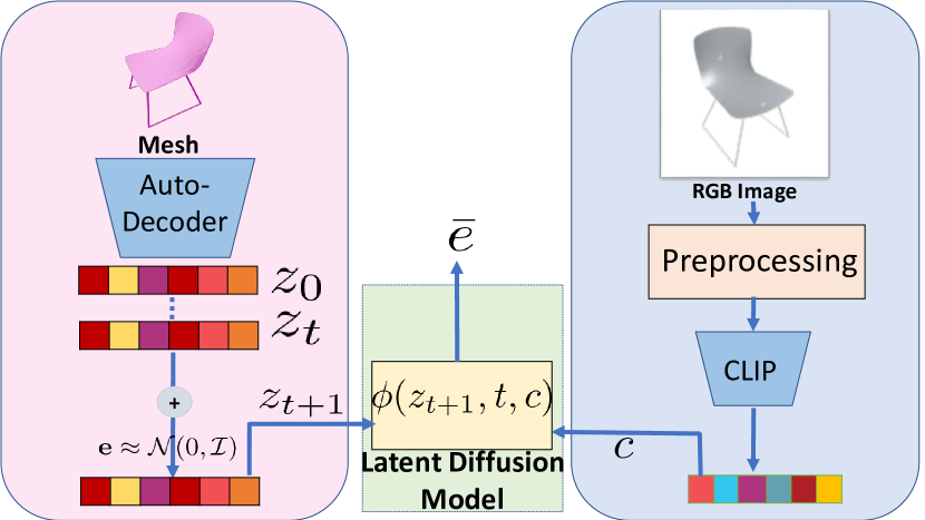
Figure 3: CLIP-conditioned version of 3D-LDM. We use a CLIP embedding of a given image or text prompt as additional input for our network $\epsilon_{\phi}$.

Training setup.

We train on image embeddings only. Since CLIP has a shared text/image latent space, we can condition the trained model on text as well. Images for training are obtained by rendering each shape in our dataset from a random camera pose.

4 Results

We evaluate 3D-LDM on unconditional generation and generation conditioned on text and images. Additionally, we show that 3D-LDM can assist in shape exploration by proposing variations of a given shape.

Implementation and Training Details.

Our latent shape vectors ${\bm{z}}$ are $256$-dimensional and are randomly sampled from $\mathcal{N}(0,0.01)$. Similar to DeepSDF [42], we are using an autodecoder with $8$ fully connected layers and $512$-dimensional hidden features. We set the regularization factor $\lambda=100$. When generating samples, we run the inverse process for $30$k steps. We train the auto-decoder for $3000$ epochs ($\sim 1$ day on a V100 GPU), and the diffusion model for $7000$ epochs ($\sim 15$ hours on a V100 GPU).

Datasets.

We evaluate our method on ShapeNet [9], a dataset containing synthetic 3D meshes of man-made objects. We use the chairs category ($6778$ shapes total, we randomly pick $6278$/$500$ as training/test set) and airplanes category ($4045$ shapes total, $3545$/$500$ for training/testing). For each shape, we pre-compute $500$k signed distance samples, using the sampling strategy and approximate inside/outside computation described in DeepSDF [42]. At training time, we evaluate our autodecoder on random subsets of $\sim 16$k samples for each shape in a batch, picked to have a balanced number of positive and negative SDF values.

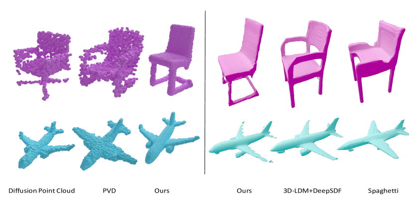
Figure 4: Qualitative comparison. Examples of generated shapes with 3D-LDM (ours) compared to other baselines. We show both the surfaces and the point clouds from our method to compare to both baselines categories. Additional qualitative results are shown in Section C.

4.1 Unconditional Generation

We generate shapes unconditionally by starting from a noisy latent shape vector ${\bm{z}}^{T}\sim\mathcal{N}(0,\mathbf{I})$ and denoising it using the reverse process described in Section 3.2. The denoised latent vector is decoded with our autodecoder into an SDF that can be converted into a meshed surface $S$ with Marching Cubes [32].

Table 1: Quantitative comparison of unconditional generation. We compare to three baselines (top group) and three ablations (bottom group). We achieve performance close to PointDiffusion, while generating neural implicit representations that can accurately represent surfaces instead of point clouds, and outperform the other baselines. We multiply MMD by $10^{3}$ and the EMD by $10^{2}$.

	Chairs						Airplanes
	MMD$\downarrow$		COV(%)$\uparrow$		1-NNA(%)$\downarrow$		MMD$\downarrow$		COV(%)$\uparrow$		1-NNA(%)$\downarrow$
	CD	EMD	CD	EMD	CD	EMD	CD	EMD	CD	EMD	CD	EMD
Point Diffusion [33]	13.6	7.52	47.8	46.0	60.0	69.9	3.3	3.33	48.4	48.2	66.5	70.9
Spaghetti [19]	18.6	8.7	42.4	43.8	66.99	72.4	4.4	3.74	44.07	41.0	78.76	81.17
PVD [72]	18.3	9.1	33.0	33.6	74.6	78.7	4.0	3.61	36.2	37.2	88.2	93.39
DeepSDF[42]	44.9	45.0	12.0	11.6	94.6	94.4	8.4	5.35	21.6	18	95.1	96.1
Our AutoDecoder	59.8	19.96	7.4	6.6	95.3	95.4	7.8	5.26	20.2	14	94.6	96.8
3D-LDM +DeepSDF	15.8	8.27	43.4	42.6	61.7	67.59	3.9	3.61	39.46	37.6	78.8	82.3
3D-LDM (ours)	16.8	8.2	42.6	42.2	58.9	65.3	4.0	3.52	46.2	42.6	74	80.1

Baselines.

We compare our results to three state-of-the-art 3D shape generators: Point Diffusion [33] directly applies the forward and reverse diffusion process to point clouds; PVD [72] applies a diffusion model to a hybrid point-voxel representation; and SPAGHETTI [19] uses a part-aware GAN on neural implicit shapes. Additionally, we compare to three ablations of our method: sampling from a Gaussian fitted to the latent shape vectors ${\bm{z}}_{i}$, sampling from a Gaussian fitted to the latent vectors of DeepSDF [42], and using our method with the original DeepSDF as autodecoder instead of our slightly modified version. We use pre-trained versions of SPAGHETTI and PVD that were trained on the same dataset and categories. We use the test set provided in their code to compute metrics, taking care to have the same shape scaling to get comparable results. We re-train Point Diffusion and the ablations on our dataset.

Metrics.

To quantitatively evaluate how similar a distribution of generated shapes is to the dataset distribution, we generate a set of $500$ shapes $\mathcal{S}_{g}$ and compare it to a set $\mathcal{S}_{t}$ of $500$ shapes from the test set, using metrics introduced in previous works on 3D shape generation [19, 67, 15]:

• Minimum Matching Distance (MMD): Measures how far test samples are from generated samples:

  $$\operatorname{MMD}\left(\mathcal{S}_{g},\mathcal{S}_{t}\right)\coloneqq\frac{1}{\left|S_{t}\right|}\sum_{Y\in S_{t}}\min_{X\in S_{g}}D(X,Y),$$ (14)

  where $D(x,y)$ is a shape distance we will define below.

• Coverage (COV): Measures what percentage of test samples are covered by generated samples. A test sample is covered if it is the nearest neighbor of a generated sample:

  $$\operatorname{COV}\left(\mathcal{S}_{g},\mathcal{S}_{t}\right)\coloneqq 100\ \frac{|\mathcal{S}_{t}\cap\{\operatorname{NN}^{D}_{\mathcal{S}_{t}\cup\mathcal{S}_{g}}(S)\mid S\in\mathcal{S}_{g}\}|}{|\mathcal{S}_{t}|},$$ (15)

  where $\operatorname{NN}^{D}_{\mathcal{X}}(Y)$ is the nearest neighbor of $Y$ in $\mathcal{X}$ according to distance metric $D$.

• Nearest Neighbour (1-NNA) Measures how well test samples and generated samples are mixed by penalizing samples from the test set and generated set that have their nearest neighbor in the same set.

We show results for the Chamfer Distance (CD) [3, 14] and the Earth Mover’s distance (EMD) [49] as metric $D$. Both operate on $2048$ uniform point samples from the shape surfaces $S$.

Table 2: Time Complexity of the generation process per shape

	Point Diffusion[33]	PVD[72]	3D-LDM (ours)
Time (s)	0.073	62.05	53.3

Results.

Table 1 shows a quantitative comparison to the baselines. PointDiffusion and PVD generate point clouds as shape representation, while SPAGHETTI and 3D-LDM create neural implicit shapes that allow for an accurate representation of the surface. We achieve performance close to PointDiffusion, while also having an accurate surface representation, and improve upon both PVD and SPAGHETTI. In the ablations, we can see that using a diffusion model to generate shape latent codes is significantly better than sampling them from a Gaussian fitted to the shape codes in the training set (DeepSDF and our AutoDecoder). We can also see that our architectural changes of the autodecoder result in a slight performance improvement over directly using DeepSDF as autodecoder (3D-LDM + DeepSDF).

In Figure 4, we showcase examples of generated instances for chair and airplane categories. Additional qualitative examples are provided in Section C of the supplementary material. We also provide results that show that our model does not overfit to the training data by comparing the generated shapes to their closest match in the training distribution. Further details are provided in Section D of the supplementary material.

Computational Complexity.

Table 2 compares the computational complexity, i.e. the time required for a single shape synthesis, of our method to several baselines[33, 72].

4.2 Conditional Generation

We additionally evaluate our diffusion model conditioned on CLIP embeddings. The goal is to learn how to retrieve the best matching shapes given an input image or text prompt. We train with images of ShapeNet chairs rendered from random camera poses, as in [12], encoded with CLIP[45]. We showcase the obtained 3D shapes in Fig 6, for each input image, we generate multiple shapes by using different random samples for the initial noise ${\bm{z}}^{T}$.

We further repeat the experiment on text prompts and test the capability of our model to generate shapes matching the prompt. Note that the model does not need to be re-trained for this task, we use the same model that was trained with encoded images. While some works have focused on category inspired prompts having the form ”This is a sofa” or ”this is a desk chair”, we have evaluated our model against more descriptive text prompts. We can see that our model conditioned on CLIP yields shapes obeying the description while varying in overall appearance. We present a few examples in Figure 5 showing chairs with wheels or chairs that look like a bed. In the second example, we can see that the chairs are larger and more comfortable.

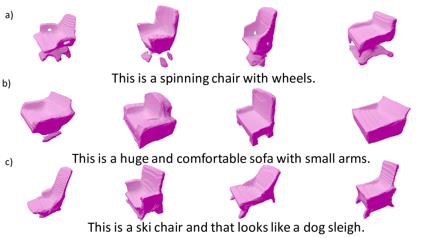
Figure 5: Text-to-Shape. 3D-LDM conditioned on CLIP embeddings can generate shapes that match the description given by the text prompt. In each row, we showcase multiple shapes generated by our model for each text prompt.

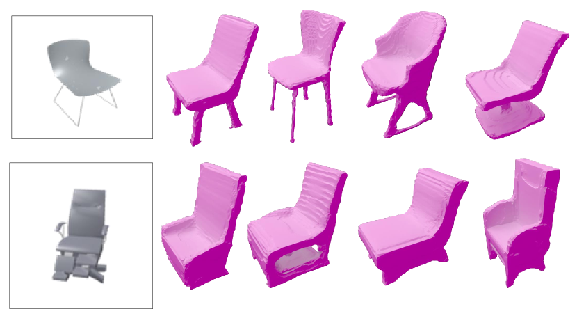
Figure 6: Image-to-Shape. 3D-LDM conditioned on CLIP embeddings can generate shapes similar to an input image. In each row, we showcase multiple shapes generated by our model for two different image renderings of chairs extracted from the chairs dataset.

4.3 Guided Shape Exploration

A fundamental variable of a Diffusion Model is the maximum number of time-steps during the noising/denoising process. The number of time-steps $T$ used to transform the distribution of latent shape vectors $z^{0}$ to the standard normal distribution needs to be pre-defined.

Generation of new shapes from scratch typically starts from pure noise at $t=T$. Given an initial latent code, however, we can explore variations of the corresponding shape by adding moderate amounts of noise $t<T$. The amount of added noise defines how similar the generated shape will be to the given initial shape. For $t\approx\mathcal{T}$, we obtain a randomly generated shape unrelated to the original whereas for $t<<\mathcal{T}$, the generated shape is identical to the initial shape. By choosing t to be moderately high, we obtain variations of the original shape where the differences amount to local styling properties.

We conduct an experiment with 2000 steps of added noise and show examples in Figure 7.

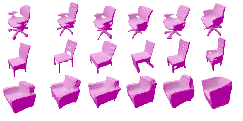
Figure 7: Guided shape exploration. By adding noise to the input shape (left column), we can generate variations of the input shapes that can be used for shape exploration. In each column, we show a different generated sample after adding 2000 noise steps to the input shape. We can see that the coarse shape of the input is preserved, but each variation generates different shape detail.

5 Conclusions

We have introduced 3D-LDM, a deep generative latent diffusion model for 3D shape generation for neural implicit functions. 3D-LDM captures the distribution of the implicit representation of the SDF in a two-stage training. First, we trained the DeepSDF auto-decoder and then the Latent Diffusion Model on the latent space of the auto-decoder to ensure better generalization and fidelity for 3D content generation. As a result, 3D-LDM ensures a performance on par with point cloud based diffusion models. Additionally, our model can be conditioned on text and images, and enables shape guided exploration by carefully adding and removing noise from the shapes.

In the future, several interesting directions could be explored. First, we could jointly train on multiple categories instead of a single category to exploit the more accurate coverage of the data distribution that a diffusion model can provide over a traditional GAN. Second, we could generate textured scenes by adding a color output in addition to the signed distance. Finally, exploring NeRF generation by adding a differentiable volume renderer to our pipeline and training with multi-view images as supervision seems like an interesting direction.

Appendix A Overview

In the following, we provide additional architecture and implementation details (Section B), provide a qualitative comparison between 3D-LDM and existing methods (Section C), evaluate the novelty of generated shapes by showing the nearest neighbors for a few generated shapes (Section D) and provide ablations for the choice of hyperparameters for our diffusion model (Section E). We will publish both the code and data we used for training.

Appendix B Implementation Details

Autodecoder Architecture

We follow the architecture of DeepSDF [42] for our autodecoder, with a few changes. Like DeepSDF, we use an MLP with $8$ fully-connected layers, a $512$-dimensional feature space for hidden layers, and a skip connection from the input to the fourth hidden layer. Unlike DeepSDF, we do not use Dropout [58] or weight normalization [51], and remove the tanh activation from the final layer, directly using the linear output instead. Empirically, we observed that this improves the quality and diversity of our generated shapes.

Denoiser Architecture

The denoiser uses an MLP consisting of $8$ linear layers with softplus activations, $512$-dimensional hidden features, and three skip connections that concatenate the output of the first hidden layer to the input of hidden layers number $3$, $5$ and $7$. Additionally, each layer is conditioned on an embedding of the denoising step $t$. Similar to DDPM [21], we use a sinusoidal embedding [62] of the time step. Additionally, each layer of the MLP, except for the first layer, transforms the time step embedding independently using a linear layer with SiLU activation [18] before adding it to the layer input. Further details about the chosen hyperparameters for training the diffusion model are presented in Section E.

Additional Autodecoder Training Details

To train our autodecoder, we use the training setup of DeepSDF [42]. We minimize the loss in Eq. 4 of our main paper using the Adam optimizer. For the point distribution of sample points $\mathcal{P}$, we use the same approach as in DeepSDF and pre-compute $500$k sample points that we randomly choose at training time. From these $500$k points, $5\%$ are uniformly distributed in the bounding box of a shape, and the rest is sampled near exterior surfaces of the shape. Exterior surfaces are identified as surfaces that are visible from a set of viewpoints $\mathcal{V}$ in a unit sphere around the shape. Points are first sampled on the exterior surfaces as intersection points of rays in view frustums that originate at viewpoints $\mathcal{V}$ and point at the origin, and then perturbed with Gaussian noise. Half of the surface points are perturbed with variance $2.510-3$, the other half with variance $2.510-4$. At training time, we create batches by randomly sampling a subset of $16$k points per shape.

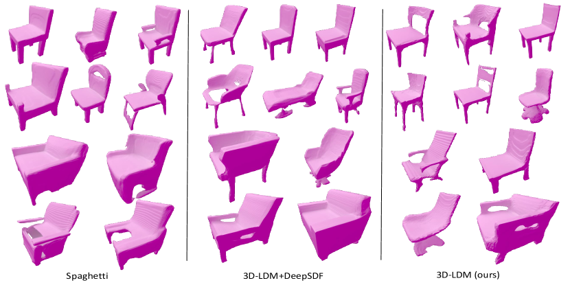
Figure 8: Qualitative comparison of generated shapes on ShapeNet Chairs. We compare $10$ randomly picked shapes generated by our method to $10$ shapes generated by each of the baselines returning surfaces similar to our method. For 3D-LDM, 3D-LDM +DeepSDF and SPAGHETTI [19], we visualize the 0-level set of the neural implicit representation (via a mesh extracted by Marching Cubes [32]).

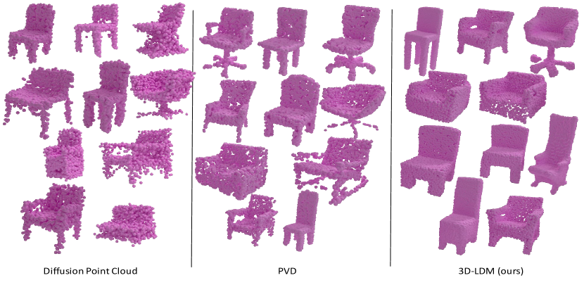
Figure 9: Qualitative comparison between 10 chairs generated by our model, picked at random from a subset of generated shapes, with point-cloud based methods from the baselines: Point Diffusion [34] and PVD [72].

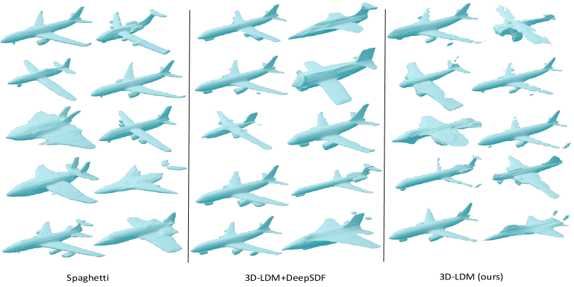
Figure 10: Qualitative comparison of generated shapes on ShapeNet Airplanes. We compare $10$ randomly picked shapes generated by our method to $10$ shapes generated by each of the baselines returning surfaces similar to our method. For 3D-LDM, 3D-LDM +DeepSDF and SPAGHETTI [19], we visualize the 0-level set of the neural implicit representation (via a mesh extracted by Marching Cubes [32]).

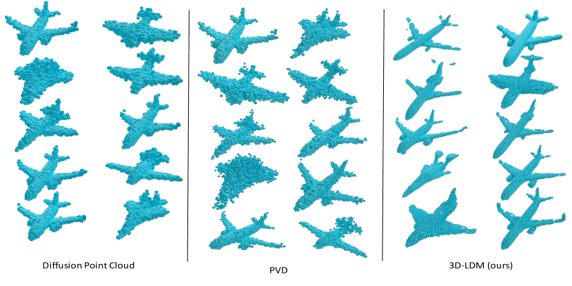
Figure 11: Qualitative comparison between 10 airplanes generated by our model, picked at random from a subset of generated shapes, with point-cloud based methods from the baselines: Point Diffusion [34] and PVD [72].

Appendix C Qualitative Comparison

In Figures 8,  10,  9 and  11, we compare $10$ uncurated shapes from our method and each of the baselines, on the Chairs and Airplanes categories, respectively.

Since PVD [72] and Point Diffusion [33] create point clouds, we separately visualize their results compared to 3D-LDM as point clouds in Figures 9 and  11.
For 3D-LDM, 3D-LDM +DeepSDF and SPAGHETTI, we visualize the surfaces reconstructed with Marching Cubes [32] from the 0-level set of the neural implicit representation. We note that the shape quality is comparable across methods, with some artifacts in the results of each method. Recall that the quantitative results in Table 1 suggest that our generated distribution better covers the data distribution, i.e. the generated shapes better reflect the variety of shapes available in the data. While this is hard to show with a limited set of uncurated samples, we can see some indication of this behaviour in the chair examples, where our results also contain types of chairs that are less common in the dataset such as swivel chairs and deck chairs, in addition to the more common dining chairs and sofa chairs, while the examples from Spaghetti consist mainly of the more common chair types.
While in the methods showcasing surfaces we detect discontinuities, point-cloud based methods usually remain noisy even after the denoising process is fully executed as we can clearly see in the generated shapes by PVD and Point Diffusion. However, these methods tend to have a superior synthesis capability than most methods which can be seen through the variety of shapes in Figures  9 and  11. This synthesis quality is also valid for our approach 3D-LDM which ensures good shape generation as supported by Table  1 and additionally provides better distributed points with minimal outliers giving the shape a nicer appearance. Figures 8,  10,  9,  11 and Table  1 show that with our method, we have a good variety of shapes, so overall it’s on par with the popular diffusion-on-point-clouds methods, while also offering the possibility to directly visualize surfaces and get good quality of point distribution with minimal outliers.

Appendix D Shape Novelty

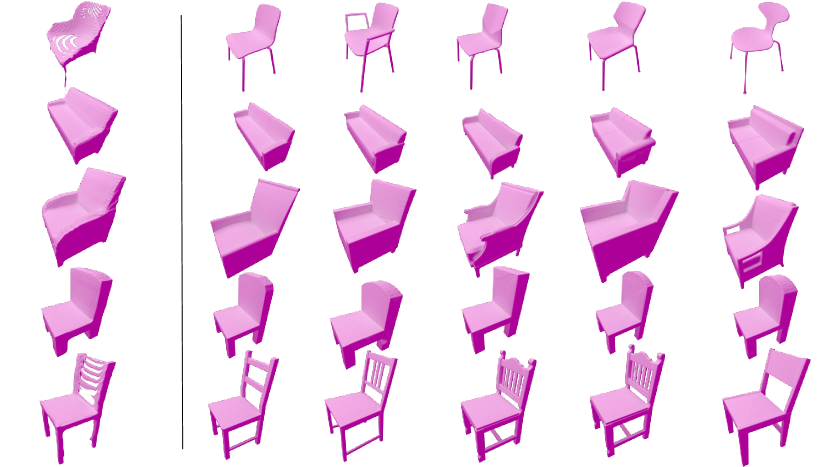
Figure 12: Novelty of generated shapes. We compare five randomly picked generated shapes to the five nearest neighbors in the training set, according to the Cosine Similarity. We can see that the generated shapes are significantly different from the training shapes, showing that our generated shapes are novel.

In Figure 12, we evaluate the novelty of our generated shapes by comparing $5$ randomly chosen generated shapes (denoted by the latent codes $\mathbf{c_{i}}$) to their $5$ nearest neighbors (NN) in the training set (denoted by the latent codes $\mathbf{c_{j}}$) , using the Cosine Similarity as metric:

$$NN(\mathbf{c_{i}})=\max_{j}cos(\mathbf{c_{i}},\mathbf{c_{j}})=\max_{j}\frac{<\mathbf{c_{i}},\mathbf{c_{j}}>}{||\mathbf{c_{i}}||.|||\mathbf{c_{j}}|}$$

The generated shapes have clear differences to their nearest neighbors in the training set, showing that the these generated shapes are indeed novel.

Table 3: Results of evaluation of different models for different hyperparameters. These metrics use the Chamfer Distance. We multiply MMD by $10^{3}$.

Hyperparameters				Metrics
Learning Rate	Batch Size	Timesteps		MMD$\downarrow$	COV$\uparrow$	1-NNA$\downarrow$
1e-4	10	30000		13.0	37.0	71.0
1e-5	10	30000		11.3	48.0	57.0
1e-6	10	30000		13.8	30.0	73.5
1e-4	24	30000		12.7	39.0	66.0
1e-5	24	30000		12.4	44.0	61.5
1e-5	24	10000		30.9	9.0	93.5

Appendix E Hyperparameter Ablations

In Table 3, we compare the performance of our approach under different hyperparameter settings. We show different settings for the learning rate, the batch size, and the total number of denoising steps.

Results show that $30$k steps significantly increase the quality of generated shapes compared to $10$k steps. We empirically observed that a smaller batch size improves results and noticed an optimum for the learning rate $110-5$. For all our experiments, we use the best-performing hyperparameter setting.
The approach we adopted to choose between the hyperparameters was by generating 100 chairs with every model and then computing the following metrics which we have described in the main paper: MMD, COV and 1-NNA between the generated shapes and a reference set from the original data. The model scoring the lowest MMD and 1-NNA, and the highest COV values is the model which hyperparameters will be the reference for training our 3D-LDM models.

References

- [1] Panos Achlioptas, Olga Diamanti, Ioannis Mitliagkas, and Leonidas Guibas. Learning representations and generative models for 3d point clouds. In International conference on machine learning, pages 40–49. PMLR, 2018.
- [2] Arpit Bansal, Eitan Borgnia, Hong-Min Chu, Jie S. Li, Hamid Kazemi, Furong Huang, Micah Goldblum, Jonas Geiping, and Tom Goldstein. Cold diffusion: Inverting arbitrary image transforms without noise, 2022.
- [3] H. G. Barrow, J. M. Tenenbaum, R. C. Bolles, and H. C. Wolf. Parametric correspondence and chamfer matching: Two new techniques for image matching. In Proceedings of the 5th International Joint Conference on Artificial Intelligence - Volume 2, IJCAI’77, pages 659–663, San Francisco, CA, USA, 1977. Morgan Kaufmann Publishers Inc.
- [4] Miguel Angel Bautista, Pengsheng Guo, Samira Abnar, Walter Talbott, Alexander Toshev, Zhuoyuan Chen, Laurent Dinh, Shuangfei Zhai, Hanlin Goh, Daniel Ulbricht, Afshin Dehghan, and Josh Susskind. Gaudi: A neural architect for immersive 3d scene generation, 2022.
- [5] Andrew Brock, Theodore Lim, James M Ritchie, and Nick Weston. Generative and discriminative voxel modeling with convolutional neural networks. arXiv preprint arXiv:1608.04236, 2016.
- [6] Ruojin Cai, Guandao Yang, Hadar Averbuch-Elor, Zekun Hao, Serge Belongie, Noah Snavely, and Bharath Hariharan. Learning gradient fields for shape generation. In European Conference on Computer Vision, pages 364–381. Springer, 2020.
- [7] Ruojin Cai, Guandao Yang, Hadar Averbuch-Elor, Zekun Hao, Serge Belongie, Noah Snavely, and Bharath Hariharan. Learning gradient fields for shape generation. In Proceedings of the European Conference on Computer Vision (ECCV), 2020.
- [8] Eric R. Chan, Marco Monteiro, Petr Kellnhofer, Jiajun Wu, and Gordon Wetzstein. pi-gan: Periodic implicit generative adversarial networks for 3d-aware image synthesis. 2021 IEEE/CVF Conference on Computer Vision and Pattern Recognition (CVPR), Jun 2021.
- [9] Angel X. Chang, Thomas Funkhouser, Leonidas Guibas, Pat Hanrahan, Qixing Huang, Zimo Li, Silvio Savarese, Manolis Savva, Shuran Song, Hao Su, Jianxiong Xiao, Li Yi, and Fisher Yu. ShapeNet: An Information-Rich 3D Model Repository. Technical Report arXiv:1512.03012 [cs.GR], Stanford University — Princeton University — Toyota Technological Institute at Chicago, 2015.
- [10] Nanxin Chen, Yu Zhang, Heiga Zen, Ron J Weiss, Mohammad Norouzi, and William Chan. Wavegrad: Estimating gradients for waveform generation. arXiv preprint arXiv:2009.00713, 2020.
- [11] Zhiqin Chen and Hao Zhang. Learning implicit fields for generative shape modeling. In Proceedings of the IEEE/CVF Conference on Computer Vision and Pattern Recognition (CVPR), June 2019.
- [12] Christopher B. Choy, Danfei Xu, JunYoung Gwak, Kevin Chen, and Silvio Savarese. 3d-r2n2: A unified approach for single and multi-view 3d object reconstruction. Lecture Notes in Computer Science, page 628–644, 2016.
- [13] Prafulla Dhariwal and Alex Nichol. Diffusion models beat gans on image synthesis. CoRR, abs/2105.05233, 2021.
- [14] Haoqiang Fan, Hao Su, and Leonidas J Guibas. A point set generation network for 3d object reconstruction from a single image. In Proceedings of the IEEE conference on computer vision and pattern recognition, pages 605–613, 2017.
- [15] Rinon Gal, Amit Bermano, Hao Zhang, and Daniel Cohen-Or. Mrgan: Multi-rooted 3d shape representation learning with unsupervised part disentanglement. In Proceedings of the IEEE/CVF International Conference on Computer Vision, pages 2039–2048, 2021.
- [16] Jun Gao, Tianchang Shen, Zian Wang, Wenzheng Chen, Kangxue Yin, Daiqing Li, Or Litany, Zan Gojcic, and Sanja Fidler. Get3d: A generative model of high quality 3d textured shapes learned from images. In Advances In Neural Information Processing Systems, 2022.
- [17] Zekun Hao, Hadar Averbuch-Elor, Noah Snavely, and Serge Belongie. Dualsdf: Semantic shape manipulation using a two-level representation. Proceedings of the IEEE/CVF Conference on Computer Vision and Pattern Recognition, pages 7631–7641, 2020.
- [18] Dan Hendrycks and Kevin Gimpel. Gaussian error linear units (gelus). arXiv preprint arXiv:1606.08415, 2016.
- [19] Amir Hertz, Or Perel, Raja Giryes, Olga Sorkine-Hornung, and Daniel Cohen-Or. Spaghetti: Editing implicit shapes through part aware generation. arXiv preprint arXiv:2201.13168, 2022.
- [20] Jonathan Ho, William Chan, Chitwan Saharia, Jay Whang, Ruiqi Gao, Alexey Gritsenko, Diederik P. Kingma, Ben Poole, Mohammad Norouzi, David J. Fleet, and Tim Salimans. Imagen video: High definition video generation with diffusion models, 2022.
- [21] Jonathan Ho, Ajay Jain, and Pieter Abbeel. Denoising diffusion probabilistic models. CoRR, abs/2006.11239, 2020.
- [22] Jonathan Ho, Chitwan Saharia, William Chan, David J Fleet, Mohammad Norouzi, and Tim Salimans. Cascaded diffusion models for high fidelity image generation. arXiv preprint arXiv:2106.15282, 2021.
- [23] Jonathan Ho and Tim Salimans. Classifier-free diffusion guidance. In NeurIPS 2021 Workshop on Deep Generative Models and Downstream Applications, 2021.
- [24] Ka-Hei Hui, Ruihui Li, Jingyu Hu, and Chi-Wing Fu. Neural wavelet-domain diffusion for 3d shape generation. arXiv preprint arXiv:2209.08725, 2022.
- [25] Ajay Jain, Ben Mildenhall, Jonathan T. Barron, Pieter Abbeel, and Ben Poole. Zero-shot text-guided object generation with dream fields. In Proceedings of the IEEE/CVF Conference on Computer Vision and Pattern Recognition (CVPR), pages 867–876, June 2022.
- [26] Nasir Mohammad Khalid, Tianhao Xie, Eugene Belilovsky, and Tiberiu Popa. Clip-mesh: Generating textured meshes from text using pretrained image-text models, 2022.
- [27] Hyeongju Kim, Hyeonseung Lee, Woo Hyun Kang, Joun Yeop Lee, and Nam Soo Kim. Softflow: Probabilistic framework for normalizing flow on manifolds. In H. Larochelle, M. Ranzato, R. Hadsell, M.F. Balcan, and H. Lin, editors, Advances in Neural Information Processing Systems, volume 33, pages 16388–16397. Curran Associates, Inc., 2020.
- [28] R. Klokov, E. Boyer, and J. Verbeek. Discrete point flow networks for efficient point cloud generation. In Proceedings of the 16th European Conference on Computer Vision (ECCV), 2020.
- [29] Zhifeng Kong, Wei Ping, Jiaji Huang, Kexin Zhao, and Bryan Catanzaro. Diffwave: A versatile diffusion model for audio synthesis. arXiv preprint arXiv:2009.09761, 2020.
- [30] Chun-Liang Li, Manzil Zaheer, Yang Zhang, Barnabas Poczos, and Ruslan Salakhutdinov. Point cloud gan. arXiv preprint arXiv:1810.05795, 2018.
- [31] Yahui Liu, Yajing Chen, Linchao Bao, Nicu Sebe, Bruno Lepri, and Marco De Nadai. Isf-gan: An implicit style function for high resolution image-to-image translation. IEEE Transactions on Multimedia, page 1–1, 2022.
- [32] William E. Lorensen and Harvey E. Cline. Marching cubes: A high resolution 3d surface construction algorithm. SIGGRAPH Comput. Graph., 21(4):163–169, 1987.
- [33] Shitong Luo and Wei Hu. Diffusion probabilistic models for 3d point cloud generation. In Proceedings of the IEEE/CVF Conference on Computer Vision and Pattern Recognition, pages 2837–2845, 2021.
- [34] Shitong Luo and Wei Hu. Diffusion probabilistic models for 3d point cloud generation. 2021 IEEE/CVF Conference on Computer Vision and Pattern Recognition (CVPR), Jun 2021.
- [35] Chenlin Meng, Yang Song, Jiaming Song, Jiajun Wu, Jun-Yan Zhu, and Stefano Ermon. Sdedit: Image synthesis and editing with stochastic differential equations. CoRR, abs/2108.01073, 2021.
- [36] Lars Mescheder, Michael Oechsle, Michael Niemeyer, Sebastian Nowozin, and Andreas Geiger. Occupancy networks: Learning 3d reconstruction in function space. In Proceedings IEEE Conf. on Computer Vision and Pattern Recognition (CVPR), 2019.
- [37] Oscar Michel, Roi Bar-On, Richard Liu, Sagie Benaim, and Rana Hanocka. Text2mesh: Text-driven neural stylization for meshes. 2022 IEEE/CVF Conference on Computer Vision and Pattern Recognition (CVPR), Jun 2022.
- [38] Ben Mildenhall, Pratul P. Srinivasan, Matthew Tancik, Jonathan T. Barron, Ravi Ramamoorthi, and Ren Ng. Nerf: Representing scenes as neural radiance fields for view synthesis. In ECCV, 2020.
- [39] Paritosh Mittal, Yen-Chi Cheng, Maneesh Singh, and Shubham Tulsiani. Autosdf: Shape priors for 3d completion, reconstruction and generation. 2022 IEEE/CVF Conference on Computer Vision and Pattern Recognition (CVPR), Jun 2022.
- [40] Alex Nichol, Prafulla Dhariwal, Aditya Ramesh, Pranav Shyam, Pamela Mishkin, Bob McGrew, Ilya Sutskever, and Mark Chen. Glide: Towards photorealistic image generation and editing with text-guided diffusion models, 2021.
- [41] Kushagra Pandey, Avideep Mukherjee, Piyush Rai, and Abhishek Kumar. VAEs meet diffusion models: Efficient and high-fidelity generation. In NeurIPS 2021 Workshop on Deep Generative Models and Downstream Applications, 2021.
- [42] Jeong Joon Park, Peter Florence, Julian Straub, Richard A. Newcombe, and Steven Lovegrove. Deepsdf: Learning continuous signed distance functions for shape representation. CoRR, abs/1901.05103, 2019.
- [43] Songyou Peng, Chiyu ”Max” Jiang, Yiyi Liao, Michael Niemeyer, Marc Pollefeys, and Andreas Geiger. Shape as points: A differentiable poisson solver. In Advances in Neural Information Processing Systems (NeurIPS), 2021.
- [44] Ben Poole, Ajay Jain, Jonathan T. Barron, and Ben Mildenhall. Dreamfusion: Text-to-3d using 2d diffusion, 2022.
- [45] Alec Radford, Jong Wook Kim, Chris Hallacy, Aditya Ramesh, Gabriel Goh, Sandhini Agarwal, Girish Sastry, Amanda Askell, Pamela Mishkin, Jack Clark, et al. Learning transferable visual models from natural language supervision. In International Conference on Machine Learning, pages 8748–8763. PMLR, 2021.
- [46] Aditya Ramesh, Prafulla Dhariwal, Alex Nichol, Casey Chu, and Mark Chen. Hierarchical text-conditional image generation with clip latents, 2022.
- [47] Edoardo Remelli, Artem Lukoianov, Stephan Richter, Benoit Guillard, Timur Bagautdinov, Pierre Baque, and Pascal Fua. Meshsdf: Differentiable iso-surface extraction. In H. Larochelle, M. Ranzato, R. Hadsell, M. F. Balcan, and H. Lin, editors, Advances in Neural Information Processing Systems, volume 33, pages 22468–22478. Curran Associates, Inc., 2020.
- [48] Robin Rombach, Andreas Blattmann, Dominik Lorenz, Patrick Esser, and Björn Ommer. High-resolution image synthesis with latent diffusion models. In Proceedings of the IEEE/CVF Conference on Computer Vision and Pattern Recognition, pages 10684–10695, 2022.
- [49] Yossi Rubner, Carlo Tomasi, and Leonidas J Guibas. A metric for distributions with applications to image databases. In Sixth international conference on computer vision (IEEE Cat. No. 98CH36271), pages 59–66. IEEE, 1998.
- [50] Chitwan Saharia, William Chan, Saurabh Saxena, Lala Li, Jay Whang, Emily Denton, Seyed Kamyar Seyed Ghasemipour, Burcu Karagol Ayan, S. Sara Mahdavi, Rapha Gontijo Lopes, Tim Salimans, Jonathan Ho, David J Fleet, and Mohammad Norouzi. Photorealistic text-to-image diffusion models with deep language understanding. 2022.
- [51] Tim Salimans and Durk P Kingma. Weight normalization: A simple reparameterization to accelerate training of deep neural networks. Advances in neural information processing systems, 29, 2016.
- [52] Aditya Sanghi, Hang Chu, Joseph G. Lambourne, Ye Wang, Chin-Yi Cheng, and Marco Fumero. Clip-forge: Towards zero-shot text-to-shape generation. CoRR, abs/2110.02624, 2021.
- [53] Dongwook Shu, Sung Woo Park, and Junseok Kwon. 3d point cloud generative adversarial network based on tree structured graph convolutions. 2019 IEEE/CVF International Conference on Computer Vision (ICCV), Oct 2019.
- [54] Uriel Singer, Adam Polyak, Thomas Hayes, Xi Yin, Jie An, Songyang Zhang, Qiyuan Hu, Harry Yang, Oron Ashual, Oran Gafni, Devi Parikh, Sonal Gupta, and Yaniv Taigman. Make-a-video: Text-to-video generation without text-video data, 2022.
- [55] Vedant Singh, Surgan Jandial, Ayush Chopra, Siddharth Ramesh, Balaji Krishnamurthy, and Vineeth N. Balasubramanian. On conditioning the input noise for controlled image generation with diffusion models, 2022.
- [56] Jascha Sohl-Dickstein, Eric A. Weiss, Niru Maheswaranathan, and Surya Ganguli. Deep unsupervised learning using nonequilibrium thermodynamics. In Proceedings of the 32nd International Conference on International Conference on Machine Learning - Volume 37, ICML’15, page 2256–2265. JMLR.org, 2015.
- [57] Jiaming Song, Chenlin Meng, and Stefano Ermon. Denoising diffusion implicit models, 2020.
- [58] Nitish Srivastava, Geoffrey Hinton, Alex Krizhevsky, Ilya Sutskever, and Ruslan Salakhutdinov. Dropout: a simple way to prevent neural networks from overfitting. The journal of machine learning research, 15(1):1929–1958, 2014.
- [59] Yongbin Sun, Yue Wang, Ziwei Liu, Joshua Siegel, and Sanjay Sarma. Pointgrow: Autoregressively learned point cloud generation with self-attention. In The IEEE Winter Conference on Applications of Computer Vision, pages 61–70, 2020.
- [60] Shufeng Tan and Michael L. Mayrovouniotis. Reducing data dimensionality through optimizing neural network inputs. Aiche Journal, 41:1471–1480, 1995.
- [61] Diego Valsesia, Giulia Fracastoro, and Enrico Magli. Learning localized generative models for 3d point clouds via graph convolution. In International Conference on Learning Representations, 2019.
- [62] Ashish Vaswani, Noam Shazeer, Niki Parmar, Jakob Uszkoreit, Llion Jones, Aidan N Gomez, Łukasz Kaiser, and Illia Polosukhin. Attention is all you need. Advances in neural information processing systems, 30, 2017.
- [63] Can Wang, Menglei Chai, Mingming He, Dongdong Chen, and Jing Liao. Clip-nerf: Text-and-image driven manipulation of neural radiance fields. In Proceedings of the IEEE/CVF Conference on Computer Vision and Pattern Recognition (CVPR), pages 3835–3844, June 2022.
- [64] Jun Wang, Wei (Wayne) Chen, Daicong Da, Mark Fuge, and Rahul Rai. Ih-gan: A conditional generative model for implicit surface-based inverse design of cellular structures. Computer Methods in Applied Mechanics and Engineering, 396:115060, 2022.
- [65] Jiajun Wu, Yifan Wang, Tianfan Xue, Xingyuan Sun, William T Freeman, and Joshua B Tenenbaum. MarrNet: 3D Shape Reconstruction via 2.5D Sketches. In Advances In Neural Information Processing Systems, 2017.
- [66] Jiajun Wu, Chengkai Zhang, Tianfan Xue, Bill Freeman, and Josh Tenenbaum. Learning a probabilistic latent space of object shapes via 3d generative-adversarial modeling. Advances in neural information processing systems, 29, 2016.
- [67] Guandao Yang, Xun Huang, Zekun Hao, Ming-Yu Liu, Serge Belongie, and Bharath Hariharan. Pointflow: 3d point cloud generation with continuous normalizing flows. In Proceedings of the IEEE/CVF International Conference on Computer Vision, pages 4541–4550, 2019.
- [68] Ling Yang, Zhilong Zhang, Yang Song, Shenda Hong, Runsheng Xu, Yue Zhao, Yingxia Shao, Wentao Zhang, Bin Cui, and Ming-Hsuan Yang. Diffusion models: A comprehensive survey of methods and applications, 2022.
- [69] K. Yin, Z. Chen, S. Chaudhuri, M. Fisher, V. G. Kim, and H. Zhang. Coalesce: Component assembly by learning to synthesize connections. In 2020 International Conference on 3D Vision (3DV), pages 61–70, Los Alamitos, CA, USA, nov 2020. IEEE Computer Society.
- [70] Jiahui Yu, Yuanzhong Xu, Jing Yu Koh, Thang Luong, Gunjan Baid, Zirui Wang, Vijay Vasudevan, Alexander Ku, Yinfei Yang, Burcu Karagol Ayan, Ben Hutchinson, Wei Han, Zarana Parekh, Xin Li, Han Zhang, Jason Baldridge, and Yonghui Wu. Scaling autoregressive models for content-rich text-to-image generation, 2022.
- [71] Xiaohui Zeng, Arash Vahdat, Francis Williams, Zan Gojcic, Or Litany, Sanja Fidler, and Karsten Kreis. Lion: Latent point diffusion models for 3d shape generation. arXiv preprint arXiv:2210.06978, 2022.
- [72] Linqi Zhou, Yilun Du, and Jiajun Wu. 3d shape generation and completion through point-voxel diffusion. CoRR, abs/2104.03670, 2021.