Electric strings in non-Abelian theories

Abstract

We find electric string solutions in Yang-Mills-Higgs theory.

Cosmic strings have attracted a lot of attention for nearly half a century since their discovery Nielsen and Olesen (1973); Vilenkin and Shellard (2000). Such strings carry magnetic flux and are analogous to vortices in superconductors. In contrast, strings that carry electric flux are expected to lead to confinement in QCD and classical solutions corresponding to electric strings are not known. Even if electric strings were to exist as classical solutions in a non-Abelian gauge theory, because gauge excitations (“gluons”) are massless and carry non-Abelian charge one might expect that rapid production of gluons by the Schwinger process Schwinger (1951); Cardona and Vachaspati (2021) would dissipate such strings . In view of these expectations it is surprising that electric string solutions do exist in certain non-Abelian gauge theories and are protected against the Schwinger process.

An essential element in constructing an electric string solution is that a non-Abelian electric field does not uniquely specify a gauge equivalent class of gauge fields. As Brown and Weisberger (BW) showed Brown and Weisberger (1979), there is a one parameter family of gauge inequivalent gauge fields that all result in the same electric field. Unlike a uniform non-Abelian electric field produced in analogy with Maxwell theory, BW gauge fields have been shown to be immune from decay due to Schwinger pair production Vachaspati (2022). This suggests the question: can there be string solutions containing BW gauge fields? In pure non-Abelian gauge theory, BW gauge fields do not solve the classical equations of motion. Instead they require external current and charge densities. Such external sources may arise due to quantum effects – after all the classical equations are expected to get modified due to the backreaction of quantum fluctuations – or they may be due to other fields in the system. Here we consider $SU(2)$ gauge theory with a scalar field in the fundamental representation. The same solution can be embedded in models with larger gauge group that have an $SU(2)$ subgroup Vachaspati and Barriola (1992); Barriola et al. (1994); Preskill (1992). The Lagrangian under consideration is,

$$L=-\frac{1}{4}W_{\mu\nu}^{a}W^{\mu\nu a}+|D_{\mu}\Phi|^{2}-V(\Phi)$$ (1)

where

$$W_{\mu\nu}^{a}=\partial_{\mu}W_{\nu}^{a}-\partial_{\nu}W_{\mu}^{a}+g\epsilon^{abc}W_{\mu}^{b}W_{\nu}^{c}$$ (2)

$$D_{\mu}\Phi=\partial_{\mu}\Phi-i\frac{g}{2}W_{\mu}^{a}\sigma^{a}\Phi$$ (3)

$$V(\Phi)=m^{2}|\Phi|^{2}+\lambda|\Phi|^{4}$$ (4)

where $\sigma^{a}$ are the Pauli spin matrices. The Lagrangian actually has an $SU(2)\times U(1)$ symmetry but only the $SU(2)$ is gauged, while the $U(1)$ is global. (This corresponds to the $\sin^{2}\theta_{w}=0$ limit of the electroweak model.)

The equations of motion are

$$(\partial_{\nu}+g\epsilon^{abc}W_{\nu}^{b})W^{\mu\nu c}=i\frac{g}{2}\left(\Phi^{\dagger}\sigma^{a}D^{\mu}\Phi-h.c.\right)$$ (5)

$$D^{\mu}D_{\mu}\Phi+m^{2}\Phi+2\lambda|\Phi|^{2}\Phi=0.$$ (6)

To find an electric field solution to the equations of motion, we first write the BW gauge field in temporal gauge Vachaspati (2022),

$$W_{0}^{a}=0,\ \ W^{\pm}_{\mu}=-\frac{\epsilon}{g}e^{\pm i\Omega t}f(r)\,\partial_{\mu}z,\ \ W^{3}_{\mu}=0,$$ (7)

where $W^{\pm}_{\mu}=W^{1}_{\mu}\pm iW^{2}_{\mu}$, and we have introduced a cylindrical profile function, $f(r)$, with $f(0)=1$. This gauge field needs sources as given by the right-hand side of (5). Requiring that $\Phi$ provides the currents that will produce the gauge field in (7) allows us to construct $\Phi$, which we have to make sure also satisfies (6). Some algebra shows that the required form of $\Phi$ is,

$$\Phi=\frac{\epsilon}{g}\sqrt{\frac{\Omega}{\omega}}\,f(r)\begin{pmatrix}z_{1}e^{+i\omega t}\\ z_{2}e^{-i\omega t}\end{pmatrix}$$ (8)

where $W^{\pm}_{\mu}=W^{1}_{\mu}\pm iW^{2}_{\mu}$ and $|z_{1}|^{2}+|z_{2}|^{2}=1$. Without loss of generality we take $\Omega>0$ while $\omega$ can be positive or negative. The $\Phi$ field can then provide suitable sources for the gauge field as well as satisfy its classical equation of motion provided we take

$$\Omega = m\left[4(1-4\lambda/g^{2})^{2}-1\right]^{-1/2}$$ (9)

$$\omega = 2(1-4\lambda/g^{2})\Omega$$ (10)

with restrictions that are necessary for $\Omega$ to be real, namely, for $m^{2}>0$, we need $0<\lambda<g^{2}/8$ ($\omega>0$), or $\lambda>3g^{2}/8$ ($\omega<0$), and for $m^{2}<0$, $g^{2}/8<\lambda<g^{2}/4$ ($\omega>0$) and $g^{2}/4<\lambda<3g^{2}/8$ ($\omega<0$). An explicit check (see Supplemental Material) shows that the solution is only valid for $\omega>0$, i.e. for $\lambda<g^{2}/4$. In what follows we will assume $\omega>0$. These constraints are summarized in Fig. 1.

Figure 1: Constraints on the parameters in the $m^{2}$-$8\lambda/g^{2}$ plane. The unshaded regions give imaginary $\Omega$ and are not allowed. The solution is only valid in the regions of parameter space where $\omega>0$.

The profile function satisfies the equation,

$$f^{\prime\prime}+\frac{f^{\prime}}{r}+\Omega^{2}\left(1-\frac{\epsilon^{2}}{2\omega\Omega}f^{2}\right)f=0.$$ (11)

with boundary conditions $f(0)=1$, $f^{\prime}(0)=0$.

For $\epsilon^{2}\ll 2\omega\Omega$ the solution is closely approximated by the zeroth order Bessel function, $J_{0}(\Omega r)$. For $\epsilon^{2}/2\omega\Omega>1$, there is no well-behaved solution. We define a rescaled profile $F(r)\equiv\epsilon f(r)/\sqrt{2\omega\Omega}$ and a rescaled coordinate $R=\Omega r$. A numerical solution for $F(R)$ vs. $R$ is shown in Fig. 2. The asymptotic form of the solution is approximately described by the asymptotic form of the Bessel function,

$$F(R)\sim F(0)\sqrt{\frac{2}{\pi R}}\,\cos\left(R-\frac{\pi}{4}\right),\ \ R\to\infty.$$ (12)

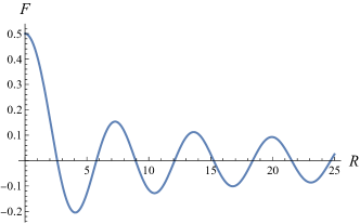
Figure 2: $F(R)$ vs. $R$ for $F(0)=0.5$.

The field strength for the solution is

$$W_{\mu\nu}^{\pm} = -\frac{\epsilon}{g}e^{\pm i\Omega t}\bigl{[}i\Omega f(r)(\partial_{\mu}t\,\partial_{\nu}z-\partial_{\nu}t\,\partial_{\mu}z)$$ (13)

$$\hskip 49.79231pt+f^{\prime}(r)(\partial_{\mu}r\,\partial_{\nu}z-\partial_{\nu}r\,\partial_{\mu}z)\bigr{]}$$

and $W_{\mu\nu}^{3}=0$. An $SU(2)$ gauge rotation by

$$U=e^{i\sigma^{1}\Omega t/2}e^{-i\sigma^{1}\pi/4}e^{-i\sigma^{2}\pi/4}$$ (14)

brings the field strength to the form,

$$W_{\mu\nu}^{\prime}=UW_{\mu\nu}U^{\dagger}$$ (15)

where $W_{\mu\nu}=W_{\mu\nu}^{a}\sigma^{a}$. This gives static field strengths of the form in Brown and Weisberger (1979) (if we set $f=1$),

$$W_{\mu\nu}^{1\,\prime}=0$$ (16)

$$W_{\mu\nu}^{2\,\prime}=-\frac{\epsilon}{g}f^{\prime}(r)(\partial_{\mu}r\,\partial_{\nu}z-\partial_{\nu}r\,\partial_{\mu}z)$$ (17)

$$W_{\mu\nu}^{3\,\prime}=-\frac{\epsilon}{g}\Omega f(r)(\partial_{\mu}t\,\partial_{\nu}z-\partial_{\nu}t\,\partial_{\mu}z)$$ (18)

Then the electric field is in the third $SU(2)$ direction and the spatial $z-$direction, while the magnetic field is in the second $SU(2)$ direction and in the spatial azimuthal direction. The structure of the solution consists of a tube of electric field along $z$, wrapped by magnetic field along the azimuthal direction $\hat{\phi}$, which is then within a sheath of electric field in the $-z$ direction, wrapped in magnetic field in the $-\hat{\phi}$ direction, and so on. The distinction between electric and magnetic fields is frame-dependent and so we calculate the Lorentz invariant $-W_{\mu\nu}^{a}W^{\mu\nu a}\propto F^{2}-F^{\prime 2}$ in Fig. 3, confirming the alternating sequence of electric and magnetic fields.

The gauge transformation $U$ when applied to $\Phi$ gives,

$$\Phi^{\prime}=U\Phi=\frac{\epsilon}{g}\sqrt{\frac{\Omega}{2\omega}}\,f(r)\begin{pmatrix}z_{1}^{\prime}e^{i\omega^{\prime}t}-z_{2}^{\prime}e^{-i\omega^{\prime}t}\\ z_{1}^{\prime}e^{i\omega^{\prime}t}+z_{2}^{\prime}e^{-i\omega^{\prime}t}\end{pmatrix}$$ (19)

where $\omega^{\prime}=\omega+\Omega/2$ and $z_{1}^{\prime}=z_{1}e^{-i\pi/4}$, $z_{2}^{\prime}=z_{2}e^{i\pi/4}$.

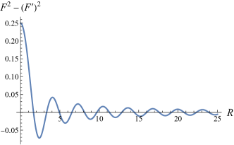
Figure 3: $F(R)^{2}-F^{\prime}(R)^{2}$ vs. $R$ for $F_{0}=0.5$. The field strength is electric-like where $F(R)^{2}-F^{\prime}(R)^{2}$ is positive and magnetic-like where $F(R)^{2}-F^{\prime}(R)^{2}$ is negative.

The energy density, ${\cal E}$ of the solution can be calculated from the expression,

$${\cal E}=\frac{1}{2}(W_{0i}^{a})^{2}+\frac{1}{4}(W_{ij}^{a})^{2}+|D_{t}\Phi|^{2}+|D_{i}\Phi|^{2}+V(\Phi)$$ (20)

In terms of rescaled variables, and restricting to $\omega>0$,

$${\cal E}^{\prime}\equiv\frac{g^{2}}{2\omega\Omega^{3}}{\cal E} = \left(\frac{1}{2}+\frac{1}{\kappa}\right)F^{\prime 2}+\left(\frac{1}{2}+2\kappa-\frac{1}{\kappa}\right)F^{2}$$ (21)

$$+\frac{1}{2}\left(\frac{1}{2}+\frac{1}{\kappa}\right)F^{4}$$

where (see (10)) $0<\kappa\equiv\omega/\Omega<2$. In Fig. 4 we show an example of ${\cal E}^{\prime}$ vs. $R$.

Figure 4: ${\cal E}^{\prime}$ vs. $R$ for $F_{0}=0.5$ and $\kappa=1.5$.

The slow fall off $\propto 1/\sqrt{R}$ of the gauge fields in (12) implies that ${\cal E}\propto 1/R$ and that the energy per unit length, $\mu$, diverges linearly with radial distance. Hence the string is not localized as in a Nielsen-Olesen string but is more like a global string that has a logarithmically divergent energy per unit length, or like a global monopole with linearly divergent energy Vilenkin and Shellard (2000). We evaluate $\mu$ numerically by integrating over $R\in[0,R_{c}]$ where $R_{c}$ is a radial cutoff to get,

$$\mu(R_{c}) = 2\pi\int_{0}^{R_{c}}dR\,R\,{\cal E}^{\prime}$$ (22)

$$\approx \left[\left(\frac{1}{2}+\frac{1}{\kappa}\right)0.54+\left(\frac{1}{2}+2\kappa-\frac{1}{\kappa}\right)0.54\right]R_{c}$$

$$+\frac{1}{2}\left(\frac{1}{2}+\frac{1}{\kappa}\right)0.09\,\ln(R_{c}),\ \ (\omega>0)$$

In the $m^{2}<0$ case, we should add a constant piece to the potential so that $V=0$ at its minimum. In that case, however, the solution still has $|\Phi|\to 0$ in the asymptotic region. Since the true vacuum has $|\Phi|\neq 0$, the solution has divergent energy per unit length and the divergence will go as $R_{c}^{2}$ instead of $R_{c}$.

Our electric string solution is with a scalar field in the fundamental representation. This leads to the question whether scalar fields in other representations can also provide suitable sources for the gauge fields in (7). We have examined the case of a scalar field in the adjoint representation, $\phi^{a}$, and can show that a solution does not exist. Briefly, the gauge field equation is $D_{\nu}W^{\mu\nu a}=j^{\mu a}$ where the current $j^{\mu a}$ is now due to the adjoint scalar and has a form such that $\phi^{a}j_{\mu}^{a}=0$ for every value of the index $\mu$. This constraint then requires $\phi^{a}D_{\nu}W^{\mu\nu a}=0$ for every $\mu$, where the gauge field is given in (7). The constraint is strong enough that it fixes the form of $\phi^{a}$. Then we can calculate $j_{\mu}^{a}$ using $\phi^{a}$ and we see that it does not satisfy the gauge field equation of motion: $j^{\mu a}=D_{\nu}W^{\mu\nu a}$.

Another interesting question is if electric string solutions exist in the electroweak model. The difference between the model in (1) and the bosonic sector of the electroweak model is that the global $U(1)$ symmetry of (1) is now gauged with coupling $g^{\prime}$ and $\Phi$ has non-vanishing $U(1)$ gauge charge (known as “hypercharge”). Then the $U(1)$ hypercharge current is,

$$j_{\mu}^{Y}=i\frac{g^{\prime}}{2}\left(\Phi^{\dagger}D_{\mu}\Phi-h.c.\right)$$ (23)

Using (7) and (8) we find,

$$j_{\mu}^{Y} = -\frac{g^{\prime}\epsilon^{2}}{g^{2}}\Omega f^{2}(|z_{1}|^{2}-|z_{2}|^{2})\partial_{\mu}t$$ (24)

$$-\frac{g^{\prime}\epsilon^{3}}{2g^{2}}\frac{\Omega}{\omega}f^{3}\left[z_{1}z_{2}^{*}e^{i(\Omega+2\omega)t}+c.c.\right]\partial_{\mu}z,$$

which shows that in general there is a hypercharge charge density as well as a three current. If $j_{\mu}^{Y}$ is non-vanishing, then necessarily the hypercharge gauge field, $Y^{\mu}$, is non-vanishing because it satisfies,

$$\partial_{\nu}Y^{\mu\nu}=j^{Y\mu}.$$ (25)

Our solution does not include a hypercharge component and so the question is if we can choose parameters such that $j_{\mu}^{Y}=0$. The $\mu=0$ component can be made to vanish by choosing $|z_{1}|^{2}=|z_{2}|^{2}$. The $\mu=3$ component is time dependent except if $\Omega+2\omega=0$, which corresponds to $\omega=-\Omega/2<0$. Since the solution is only valid for $\omega>0$, it does not hold in the electroweak model with $Y_{\mu}=0$. An alternate possibility is that there exist solutions with non-vanishing hypercharge gauge field $Y_{\mu}$ and then we do not need to require that $j_{\mu}^{Y}$ vanish. We have not been able to construct such solutions.

An important feature of the gauge field in the solution is that it is stationary. In other words, consider perturbations of only the gauge field,

$$W_{\mu}^{\pm}=A_{\mu}^{\pm}+e^{\pm i\Omega t}Q_{\mu}^{a},\ \ W_{\mu}^{3}=Q_{\mu}^{3},\ \ \Phi=\Phi_{0}$$ (26)

where $A_{\mu}^{a}$, $\Phi_{0}$ denote the electric string solution. Then the action for $Q_{\mu}^{a}$ does not contain any terms that are explicitly time-dependent and hence the solution is protected from decay to Schwinger pair production of gauge field excitations as shown in Ref. Vachaspati (2022). The inclusion of the scalar field, $\Phi$, does not make any difference to the analysis in Ref.  Vachaspati (2022) because the quadratic order interaction between $\Phi$ and $Q_{\mu}^{a}$ is simply $g^{2}|\Phi|^{2}(Q_{\mu}^{a})^{2}/4$ and $|\Phi|^{2}$ is time-independent. (The linear order terms vanish because the solution obeys the classical equations of motion.) Fluctuations of the scalar field $\Phi$ can indeed get excited by the time dependence of the solution, and this means that Schwinger pair production of $\Phi$ excitations will occur. (This is similar to the Schwinger pair production of quarks on QCD strings.) In the limit of large mass parameter $m$, the Schwinger pair production of $\Phi$ will be suppressed.

A Maxwell electric field for example, with $W_{z}^{3}=-Et$ and all other components zero, is a classical solution of the SU(2) pure gauge theory. However, the Schwinger process for gluons in this background is non-vanishing at all momentum scales Cardona and Vachaspati (2021) and the Maxwell electric field will decay and evolve into another configuration. Since a BW electric field is stable to the Schwinger process, it is likely that it is the final state. In other words, if initially we start with a Maxwell electric field, it may evolve into a BW electric field.

In Ref. Pereira and Vachaspati (2022) the classical stability of a homogeneous electric field of the BW type was analyzed. Several unstable modes were found for the homogeneous configuration. For the electric string, these unstable modes will be suppressed due to the $|\Phi|^{2}(Q_{\mu}^{a})^{2}$ term, since this term provides an effective mass to the gauge excitations wherever $|\Phi|^{2}$ is non-zero. The solutions with $m^{2}<0$ will almost certainly be unstable since $\Phi$ approaches the unstable vacuum, $|\Phi|=0$, in the asymptotic region. We plan to carry out a detailed stability analysis in a future publication.

We close with a speculative remark. The solution we have found may be of interest in the context of pure non-Abelian gauge theories. In that case, the field $\Phi$ must arise as an effective degree of freedom due to quantum backreaction in the classical equations of motion. In this connection, it has been conjectured that magnetic monopoles at strong coupling transform as a scalar degree of freedom in the fundamental representation of a dual symmetry group Goddard et al. (1977). While there are no classical monopole solutions in pure non-Abelian gauge theory, one can still write configurations that resemble the gauge fields of magnetic monopoles,

$$W_{i}^{a}=\frac{(1-k(r))}{g\,r}\epsilon^{aij}{\hat{x}}^{j}$$ (27)

where $k(r)$ is a suitable profile function. Can the backreaction due to such monopole configurations behave like our scalar field $\Phi$ and provide the necessary sources for electric strings?

I thank Jude Pereira and Shekhar Sharma for discussions and Gia Dvali for comments. This work was supported by the U.S. Department of Energy, Office of High Energy Physics, under Award DE-SC0019470 at ASU.

Appendix A Supplemental Material

A.1 Check of solution

The solution needs to satisfy

$$(\partial_{\nu}+g\epsilon^{abc}W_{\nu}^{b})W^{\mu\nu c}=i\frac{g}{2}\left(\Phi^{\dagger}\sigma^{a}D^{\mu}\Phi-h.c.\right)$$ (28)

$$D^{\mu}D_{\mu}\Phi+m^{2}\Phi+2\lambda|\Phi|^{2}\Phi=0.$$ (29)

The solution is

$$\Phi=\frac{\epsilon}{g}\sqrt{\frac{\Omega}{\omega}}\,f(r)\begin{pmatrix}z_{1}e^{+i\omega t}\\ z_{2}e^{-i\omega t}\end{pmatrix}$$ (30)

and the only non-vanishing components of the gauge field are

$$W^{1}_{z}=-\frac{\epsilon}{g}\cos(\Omega t)f(r),\ \ W^{2}_{z}=-\frac{\epsilon}{g}\sin(\Omega t)f(r).$$ (31)

Then

$$W_{\mu\nu}^{1} = -\frac{\epsilon}{g}\bigl{[}-\Omega\sin(\Omega t)f(r)(\partial_{\mu}t\,\partial_{\nu}z-\partial_{\nu}t\,\partial_{\mu}z)$$ (32)

$$\hskip 0.0pt+\cos(\Omega t)f^{\prime}(r)(\partial_{\mu}r\,\partial_{\nu}z-\partial_{\nu}r\,\partial_{\mu}z)\bigr{]}$$

$$W_{\mu\nu}^{2} = -\frac{\epsilon}{g}\bigl{[}+\Omega\cos(\Omega t)f(r)(\partial_{\mu}t\,\partial_{\nu}z-\partial_{\nu}t\,\partial_{\mu}z)$$ (33)

$$\hskip 0.0pt+\sin(\Omega t)f^{\prime}(r)(\partial_{\mu}r\,\partial_{\nu}z-\partial_{\nu}r\,\partial_{\mu}z)\bigr{]}$$

and $W_{\mu\nu}^{3}=0$. This then gives,

$$D_{\nu}W^{\mu\nu 1} = -\frac{\epsilon}{g}\cos(\Omega t)\left[f^{\prime\prime}+\frac{f^{\prime}}{r}+\Omega^{2}f\right]\partial^{\mu}z$$ (34)

$$D_{\nu}W^{\mu\nu 2} = -\frac{\epsilon}{g}\sin(\Omega t)\left[f^{\prime\prime}+\frac{f^{\prime}}{r}+\Omega^{2}f\right]\partial^{\mu}z$$ (35)

$$D_{\nu}W^{\mu\nu 3} = -\frac{\epsilon^{2}}{g}\Omega f^{2}\partial^{\mu}t$$ (36)

where $D_{\nu}=\partial_{\nu}+g\epsilon^{abc}W_{\nu}^{b}$.

Next we calculate the current

$$j_{\mu}^{a}=i\frac{g}{2}\left(\Phi^{\dagger}\sigma^{a}D^{\mu}\Phi-h.c.\right)$$ (37)

This calculation is simplified by the identity

$$\sigma^{a}\sigma^{b}=\delta^{ab}+i\epsilon^{abc}\sigma^{c}$$ (38)

and by the observation

$$\partial_{\mu}\Phi=\left(\frac{f^{\prime}}{f}\partial_{\mu}r+i\omega\sigma_{3}\partial_{\mu}t\right)\Phi.$$ (39)

For then

$$\Phi^{\dagger}\sigma^{1}\partial_{\mu}\Phi=\frac{f^{\prime}}{f}\partial_{\mu}r\,(\Phi^{\dagger}\sigma^{1}\Phi)+\omega\partial_{\mu}t\,(i\Phi^{\dagger}\sigma^{1}\sigma^{3}\Phi).$$ (40)

Both $\Phi^{\dagger}\sigma^{1}\Phi$ and $i\Phi^{\dagger}\sigma^{1}\sigma^{3}\Phi=\Phi^{\dagger}\sigma^{2}\Phi$ are real. Therefore

$$\Phi^{\dagger}\sigma^{1}\partial_{\mu}\Phi-h.c.=0.$$ (41)

Similarly

$$\Phi^{\dagger}\sigma^{2}\partial_{\mu}\Phi-h.c.=0$$ (42)

and

$$\Phi^{\dagger}\sigma^{3}\partial_{\mu}\Phi-h.c.=2i\omega|\Phi|^{2}\partial_{\mu}t$$ (43)

Similar considerations apply to $\Phi^{\dagger}\sigma^{a}W_{\mu}^{b}\sigma^{b}\Phi$ and we get

$$\hskip-227.62204pt-i\frac{g}{2}\Phi^{\dagger}\sigma^{a}W_{\mu}^{b}\sigma^{b}\Phi-h.c.=$$

$$\left(-i\frac{g}{2}W_{\mu}^{a}|\Phi|^{2}+\frac{g}{2}\epsilon^{abc}W_{\mu}^{b}\Phi^{\dagger}\sigma^{c}\Phi\right)-h.c.=-i2gW_{\mu}^{a}|\Phi|^{2}$$

For now we consider $\omega$ to be positive or negative. Then,

$$|\Phi|^{2}=\frac{\epsilon^{2}}{g^{2}}\frac{\Omega}{|\omega|}f^{2}.$$ (44)

The currents from the $\Phi$ field are

$$j_{\mu}^{1} = \frac{g^{2}}{2}W_{\mu}^{1}|\Phi|^{2}$$ (45)

$$=-\frac{\epsilon}{g}\cos(\Omega t)\Omega^{2}\frac{\epsilon^{2}}{2|\omega|\Omega}f^{3}\partial_{\mu}z$$

$$j_{\mu}^{2} = \frac{g^{2}}{2}W_{\mu}^{1}|\Phi|^{2}$$ (46)

$$=-\frac{\epsilon}{g}\sin(\Omega t)\Omega^{2}\frac{\epsilon^{2}}{2|\omega|\Omega}f^{3}\partial_{\mu}z$$

$$j_{\mu}^{3} = -\frac{\epsilon^{2}}{g}\frac{\omega}{|\omega|}\Omega f^{2}\partial_{\mu}t$$ (47)

Matching (47) to (36) we see that it is necessary to restrict $\omega$ to be positive and hence we only consider $\omega>0$ below. Further, matching (34)-(35) with (45)-(46), we see that the gauge equations are satisfied if $f(r)$ is a solution of

$$f^{\prime\prime}+\frac{f^{\prime}}{r}+\Omega^{2}\left(1-\frac{\epsilon^{2}}{2\omega\Omega}f^{2}\right)f=0.$$ (48)

Next we come to the $\Phi$ equation of motion in (29).

$$D^{\mu}D_{\mu}\Phi = \left(\partial^{\mu}-i\frac{g}{2}W^{\mu a}\sigma^{a}\right)\left(\partial_{\mu}-i\frac{g}{2}W_{\mu}^{b}\sigma^{b}\right)\Phi$$

$$= \partial^{\mu}\partial_{\mu}\Phi-\frac{g^{2}}{4}W^{\mu a}W_{\mu}^{b}(\delta^{ab}+i\epsilon^{abc}\sigma^{c})\Phi$$

$$= \partial^{\mu}\partial_{\mu}\Phi-\frac{g^{2}}{4}W^{\mu a}W_{\mu}^{a}\Phi$$

where we have used $\partial_{\mu}W^{\mu a}=0=W^{\mu a}\partial_{\mu}\Phi$, and $\epsilon^{abc}W^{\mu a}W_{\mu}^{b}=0$. To simplify further, we use (39) to get,

$$\partial^{\mu}\partial_{\mu}\Phi = \partial^{\mu}\left(\frac{f^{\prime}}{f}\partial_{\mu}r\Phi\right)+\left(\frac{f^{\prime}}{f}\partial_{\mu}r+i\omega\sigma_{3}\partial_{\mu}t\right)^{2}\Phi$$ (49)

$$= -\left(\frac{f^{\prime\prime}}{f}+\frac{f^{\prime}}{rf}+\omega^{2}\right)\Phi$$

Therefore the equation of motion for $\Phi$ becomes

$$0 = D^{\mu}D_{\mu}\Phi+m^{2}\Phi+2\lambda|\Phi|^{2}\Phi$$

$$= -\left(f^{\prime\prime}+\frac{f^{\prime}}{r}+\omega^{2}f-\frac{\epsilon^{2}}{4}f^{3}-m^{2}f-2\lambda\frac{\epsilon^{2}}{g^{2}}\frac{\Omega}{\omega}f^{3}\right)\frac{\Phi}{f}$$

or

$$f^{\prime\prime}+\frac{f^{\prime}}{r}+(\omega^{2}-m^{2})f-\left(\frac{\epsilon^{2}}{4}+2\lambda\frac{\epsilon^{2}}{g^{2}}\frac{\Omega}{\omega}\right)f^{3}=0$$ (50)

From (9) and (10) one checks that

$$\omega^{2}-m^{2}=\Omega^{2}$$ (51)

and

$$\frac{\epsilon^{2}}{4}+2\lambda\frac{\epsilon^{2}}{g^{2}}\frac{\Omega}{\omega} = \frac{\epsilon^{2}}{4}\left(1+\frac{8\lambda}{g^{2}}\frac{\Omega}{\omega}\right)$$ (52)

$$= \frac{\epsilon^{2}}{4}\left(1+\frac{4\lambda}{g^{2}}\frac{1}{1-4\lambda/g^{2}}\right)$$

$$= \frac{\epsilon^{2}}{4(1-4\lambda/g^{2})}$$

$$= \frac{\epsilon^{2}\Omega^{2}}{2\omega\Omega}$$

Using these relations, (50) is identical to (48) and so the $\Phi$ equation is satisfied too.

References

Nielsen and Olesen (1973)
H. B. Nielsen and
P. Olesen,
Nucl. Phys. B 61,
45 (1973).
Vilenkin and Shellard (2000)
A. Vilenkin and
E. P. S. Shellard,
Cosmic Strings and Other Topological Defects
(Cambridge University Press, 2000), ISBN
978-0-521-65476-0.
Schwinger (1951)
J. S. Schwinger,
Phys. Rev. 82,
664 (1951).
Cardona and Vachaspati (2021)
C. Cardona and
T. Vachaspati,
Phys. Rev. D 104,
045009 (2021), eprint 2105.08782.
Jackiw et al. (1979)
R. Jackiw,
L. Jacobs, and
C. Rebbi,
Phys. Rev. D 20,
474 (1979).
Huang and Tipton (1981)
K. Huang and
R. Tipton,
Phys. Rev. D 23,
3050 (1981).
Brown and Weisberger (1979)
L. S. Brown and
W. I. Weisberger,
Nucl. Phys. B 157,
285 (1979), [Erratum:
Nucl.Phys.B 172, 544 (1980)].
Vachaspati (2022)
T. Vachaspati,
Phys. Rev. D 105,
105011 (2022), eprint 2204.01902.
Vachaspati and Barriola (1992)
T. Vachaspati and
M. Barriola,
Phys. Rev. Lett. 69,
1867 (1992).
Barriola et al. (1994)
M. Barriola,
T. Vachaspati,
and M. Bucher,
Phys. Rev. D 50,
2819 (1994), eprint hep-th/9306120.
Preskill (1992)
J. Preskill,
Phys. Rev. D 46,
4218 (1992), eprint hep-ph/9206216.
Workman and Others (2022)
R. L. Workman and
Others (Particle Data
Group), PTEP 2022,
083C01 (2022).
Pereira and Vachaspati (2022)
J. Pereira and
T. Vachaspati,
Phys. Rev. D 106,
096019 (2022), eprint 2207.05102.
Goddard et al. (1977)
P. Goddard,
J. Nuyts, and
D. I. Olive,
Nucl. Phys. B 125,
1 (1977).