Scaling Language-Image Pre-training via Masking

Abstract

We present Fast Language-Image Pre-training (FLIP), a simple and more efficient method for training CLIP [52]. Our method randomly masks out and removes a large portion of image patches during training. Masking allows us to learn from more image-text pairs given the same wall-clock time and contrast more samples per iteration with similar memory footprint. It leads to a favorable trade-off between accuracy and training time. In our experiments on 400 million image-text pairs, FLIP improves both accuracy and speed over the no-masking baseline. On a large diversity of downstream tasks, FLIP dominantly outperforms the CLIP counterparts trained on the same data. Facilitated by the speedup, we explore the scaling behavior of increasing the model size, data size, or training length, and report encouraging results and comparisons. We hope that our work will foster future research on scaling vision-language learning.

1 Introduction

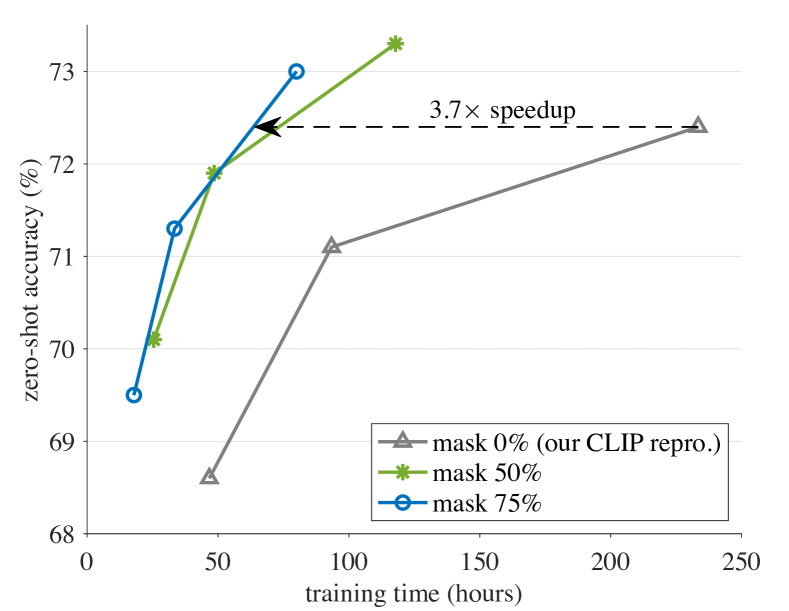
Figure 1: Accuracy vs. training time trade-off. With a high masking ratio of 50% or 75%, our FLIP method trains faster and is more accurate than its CLIP counterpart. All entries are benchmarked in 256 TPU-v3 cores. Training is done on LAION-400M for 6.4, 12.8, or 32 epochs, for each masking ratio. Accuracy is evaluated by zero-shot transfer on the ImageNet-1K validation set. The model is ViT-L/16 [20]. More details are in Fig. 3. As the CLIP baseline takes $\scriptstyle\sim$2,500 TPU-days training, a speedup of 3.7$\times$ can save $\scriptstyle\sim$1,800 TPU-days.

Language-supervised visual pre-training, e.g., CLIP [52], has been established as a simple yet powerful methodology for learning representations. Pre-trained CLIP models stand out for their remarkable versatility: they have strong zero-shot transferability [52]; they demonstrate unprecedented quality in text-to-image generation (e.g., [53, 55]); the pre-trained encoder can improve multimodal and even unimodal visual tasks. Like the role played by supervised pre-training a decade ago [40], language-supervised visual pre-training is new fuel empowering various tasks today.

Unlike classical supervised learning with a pre-defined label set, natural language provides richer forms of supervision, e.g., on objects, scenes, actions, context, and their relations, at multiple levels of granularity. Due to the complex nature of vision plus language, large-scale training is essential for the capability of language-supervised models. For example, the original CLIP models [52] were trained on 400 million data for 32 epochs—which amount to 10,000 ImageNet [16] epochs, taking thousands of GPU-days [52, 36]. Even using high-end infrastructures, the wall-clock training time is still a major bottleneck hindering explorations on scaling vision-language learning.

We present Fast Language-Image Pre-training (FLIP), a simple method for efficient CLIP training. Inspired by the sparse computation of Masked Autoencoders (MAE) [29], we randomly remove a large portion of image patches during training. This design introduces a trade-off between “how carefully we look at a sample pair” vs. “how many sample pairs we can process”. Using masking, we can: (i) see more sample pairs (i.e., more epochs) under the same wall-clock training time, and (ii) compare/contrast more sample pairs at each step (i.e., larger batches) under similar memory footprint. Empirically, the benefits of processing more sample pairs greatly outweigh the degradation of per-sample encoding, resulting in a favorable trade-off.

By removing 50%-75% patches of a training image, our method reduces computation by 2-4${\times}$; it also allows using 2-4${\times}$ larger batches with little extra memory cost, which boost accuracy thanks to the behavior of contrastive learning [30, 11]. As summarized in Fig. 1, FLIP trains $>$3${\times}$ faster in wall-clock time for reaching similar accuracy as its CLIP counterpart; with the same number of epochs, FLIP reaches higher accuracy than its CLIP counterpart while still being 2-3${\times}$ faster.

We show that FLIP is a competitive alternative to CLIP on various downstream tasks. Pre-trained on the same LAION-400M dataset [56], FLIP dominantly outperforms its CLIP counterparts (OpenCLIP [36] and our own reproduction), as evaluated on a large variety of downstream datasets and transfer scenarios. These comparisons suggest that FLIP can readily enjoy the faster training speed while still providing accuracy gains.

Facilitated by faster training, we explore scaling FLIP pre-training. We study these three axes: (i) scaling model size, (ii) scaling dataset size, or (iii) scaling training schedule length. We analyze the scaling behavior through carefully controlled experiments. We observe that model scaling and data scaling can both improve accuracy, and data scaling can show gains at no extra training cost. We hope our method, results, and analysis will encourage future research on scaling vision-language learning.

2 Related Work

Learning with masking.

Denoising Autoencoders [63] with masking noise [64] were proposed as an unsupervised representation learning method over a decade ago. One of its most outstanding applications is masked language modeling represented by BERT [18]. In computer vision, explorations along this direction include predicting large missing regions [50], sequence of pixels [10], patches [20, 29, 71], or pre-computed features [6, 66].

The Masked Autoencoder (MAE) method [29] further takes advantage of masking to reduce training time and memory. MAE sparsely applies the ViT encoder [20] to visible content. It also observes that a high masking ratio is beneficial for accuracy. The MAE design has been applied to videos [61, 22], point clouds [49], graphs [59, 9, 32], audio [4, 47, 13, 35], visual control [70, 57], vision-language [23, 41, 31, 19], and other modalities [5].

Our work is related to MAE and its vision-language extensions [23, 41, 31, 19]. However, our focus is on the scaling aspect enabled by the sparse computation; we address the challenge of large-scale CLIP training [52], while previous works [23, 41, 31, 19] are limited in terms of scale. Our method does not perform reconstruction and is not a form of autoencoding. Speeding up training by masking is studied in [69] for self-supervised contrastive learning, e.g., for MoCo [30] or BYOL [27], but its accuracy could be limited by the scaling behavior of image-only contrastive learning.

Language-supervised learning.

In the past years, CLIP [52] and related works (e.g., [37, 51]) have popularized learning visual representations with language supervision. CLIP is a form of contrastive learning [28] by comparing image-text sample pairs. Beyond contrastive learning, generative learning methods have been explored [17, 65, 2, 74], optionally combined with contrastive losses [74]. Our method focuses on the CLIP method, while we hope it can be extended to generative methods in the future.

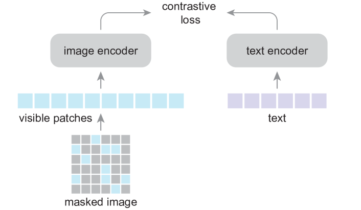
Figure 2: Our FLIP architecture. Following CLIP [52], we perform contrastive learning on pairs of image and text samples. We randomly mask out image patches with a high masking ratio and encode only the visible patches. We do not perform reconstruction of masked image content.

3 Method

In a nutshell, our method simply masks out the input data in CLIP [52] training and reduces computation. See Fig. 2.

In our scenario, the benefit of masking is on wisely spending computation. Intuitively, this leads to a trade-off between how densely we encode a sample against how many samples we compare as the learning signal. By introducing masking, we can: (i) learn from more image-text pairs under the same wall-clock training time, and (ii) have a contrastive objective over a larger batch under the same memory constraint. We show by experiments that for both aspects, our method is at an advantage in the trade-off. Next we introduce the key components of our method.

Image masking.

We adopt the Vision Transformer (ViT) [20] as the image encoder. An image is first divided into a grid of non-overlapping patches. We randomly mask out a large portion (e.g., 50% or 75%) of patches; the ViT encoder is only applied to the visible patches, following [29]. Using a masking ratio of 50% (or 75%) reduces the time complexity of image encoding to 1/2 (or 1/4); it also allows using a 2${\times}$ (or 4${\times}$) larger batch with a similar memory cost for image encoding.

Text masking.

Optionally, we perform text masking in the same way as image masking. We mask out a portion of the text tokens and apply the encoder only to the visible tokens, as in [29]. This is unlike BERT [18] that replaces them with a learned mask token. Such sparse computation can reduce the text encoding cost. However, as the text encoder is smaller [52], speeding it up does not lead to a better overall trade-off. We study text masking for ablation only.

Objective.

The image/text encoders are trained to minimize a contrastive loss [48]. The negative sample pairs for contrastive learning consist of other samples in the same batch [11]. It has been observed that a large number of negative samples is critical for self-supervised contrastive learning on images [30, 11]. This property is more prominent in language-supervised learning.

We do not use a reconstruction loss, unlike MAE [29]. We find that reconstruction is not necessary for good performance on zero-shot transfer. Waiving the decoder and reconstruction loss yields a better speedup.

Unmasking.

While the encoder is pre-trained on masked images, it can be directly applied on intact images without changes, as is done in [29]. This simple setting is sufficient to provide competitive results and will serve as our baseline in ablation experiments.

To close the distribution gap caused by masking, we can set the masking ratio as 0% and continue pre-training for a small number of steps. This unmasking tuning strategy produces a more favorable accuracy/time trade-off.

mask	batch	FLOPs	time	acc.
0%	16k	1.00${\times}$	1.00${\times}$	68.6
50%	32k	0.52${\times}$	0.50${\times}$	69.6
75%	64k	0.28${\times}$	0.33${\times}$	68.2

(a)

batch	mask 50%	mask 75%
16k	68.5	65.8
32k	69.6	67.3
64k	70.4	68.2

(b)

text mask	text len	time	acc.
baseline, 0%	32	1.00$\times$	68.2
random, 50%	16	0.92${\times}$	66.0
prioritized, 50%	16	0.92${\times}$	67.8

(c)

	mask 50%	mask 75%
w/ mask	66.4	60.9
w/ mask, ensemble	68.1	65.1
w/o mask	69.6	68.2

(d)

	mask 50%	mask 75%
baseline	69.6	68.2
+ tuning	70.1	69.5

(e)

	mask 50%	mask 75%
baseline	69.6	68.2
+ MAE	69.4	67.9

(f)

Table 1: Zero-shot ablation experiments. Pre-training is on LAION-400M for 6.4 epochs, evaluated by zero-shot classification accuracy on ImageNet-1K validation. The backbone is ViT-L/16 [20]. Unless specified, the baseline setting is: image masking is 50% (batch 32k) or 75% (batch 64k), text masking is 0%, and no unmasked tuning is used.

3.1 Implementation

Our implementation follows CLIP [52] and OpenCLIP [36], with a few modifications we describe in the following. Hyper-parameters are in the appendix.

Our image encoder follows the ViT paper [20]. We do not use the extra LayerNorm [3] after patch embedding, like [20] but unlike [52]. We use global average pooling at the end of the image encoder. The input size is 224.

Our text encoder is a non-autoregressive Transformer [62], which is easier to adapt to text masking for ablation. We use a WordPiece tokenizer as in [18]. We pad or cut the sequences to a fixed length of 32. We note that CLIP in [52] uses an autoregressive text encoder, a BytePairEncoding tokenizer, and a length of 77. These designs make marginal differences as observed in our initial reproduction.

The outputs of the image encoder and text encoder are projected to the same-dimensional embedding space by a linear layer. The cosine similarities of the embeddings, scaled by a learnable temperature parameter [52], are the input to the InfoNCE loss [48].

In zero-shot transfer, we follow the prompt engineering in the code of [52]. We use their provided 7 prompt templates for ImageNet zero-shot transfer.

Our implementation is based on JAX [8] with the t5x library [54] for large-scale distributed training. Our training is run on TPU v3 infrastructure.

4 Experiments

4.1 Ablations

We first ablate the FLIP design. The image encoder is ViT-L/16 [20], and the text encoder has a smaller size as per [52]. We train on LAION-400M [36] and evaluate zero-shot accuracy on ImageNet-1K [16] validation.

Table 1 shows the ablations trained for 6.4 epochs. Fig. 1 plots the trade-off for up to 32 epochs [52]. The results are benchmarked in 256 TPU-v3 cores, unless noted.

Masking ratio.

Table LABEL:tab:ablation:ratio studies the image masking ratios. Here we scale the batch size accordingly (ablated next), so as to roughly maintain the memory footprint.The 0% masking entry indicates our CLIP counterpart. Masking 50% gives 1.2% higher accuracy than the CLIP baseline, and masking 75% is on par with the baseline. Speed-wise, masking 50% or 75% takes only 0.50$\times$ or 0.33$\times$ wall-clock training time, thanks to the large reduction on FLOPs.

Batch size.

We ablate the effect of batch size in Table LABEL:tab:ablation:batch. Increasing the batch size consistently improves accuracy.

Notably, even using the same batch size of 16k, our 50% masking entry has a comparable accuracy (68.5%, Table LABEL:tab:ablation:batch) with the 0% masking baseline (68.6%, Table LABEL:tab:ablation:ratio). It is possible that the regularization introduced by masking can reduce overfitting, partially counteracting the negative effect of losing information in this setting. With a higher masking ratio of 75%, the negative effect is still observed when keeping the batch size unchanged.

Our masking-based method naturally encourages using large batches. There is little extra memory cost if we scale the batch size according to the masking ratio, as we report in Table LABEL:tab:ablation:ratio. In practice, the available memory is always a limitation for larger batches. For example, the setting in Table LABEL:tab:ablation:ratio has reached the memory limit in our high-end infrastructure (256 TPU-v3 cores with 16GB memory each). The memory issue is more demanding if using fewer devices, and the gain of our method would be more prominent due to the nearly free increase of batch sizes.

Text masking.

Table LABEL:tab:ablation:text studies text masking. Randomly masking 50% text decreases accuracy by 2.2%. This is in line with the observation [29] that language data has higher information-density than images and thus the text masking ratio should be lower.

As variable-length text sequences are padded to generate a fixed-length batch, we can prioritize masking out the padding tokens. Prioritized sampling preserves more valid tokens than randomly masking the padded sequences uniformly. It reduces the degradation to 0.4%.

While our text masking is more aggressive than typical masked language models (e.g., 15% in [18]), the overall speed gain is marginal. This is because the text encoder is smaller and the text sequence is short. The text encoder costs merely 4.4% computation vs. the image encoder (without masking). Under this setting, text masking is not a worthwhile trade-off and we do not mask text in our other experiments.

Inference unmasking.

By default, we apply our models on intact images at inference-time, similar to [29]. While masking creates a distribution shift between training and inference, simply ignoring this shift works surprisingly well (Table LABEL:tab:ablation:infer, ‘w/o mask’), even under the zero-shot setting where no training is ever done on full images.

Table LABEL:tab:ablation:infer reports that if using masking at inference time, the accuracy drops by a lot (e.g., 7.3%). This drop can be partially caused by information loss at inference, so we also compare with ensembling multiple masked views [10], where the views are complementary to each other and put together cover all patches. Ensembling reduces the gap (Table LABEL:tab:ablation:infer), but still lags behind the simple full-view inference.

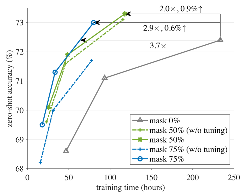
Figure 3: Accuracy vs. training time trade-off in detail. The setting follows Table LABEL:tab:ablation:ratio. Training is for 6.4, 12.8, or 32 epochs, for each masking ratio. Unmasked tuning, if applied, is for 0.32 epoch. All are benchmarked in 256 TPU-v3 cores. Zero-shot accuracy is on IN-1K validation. The model is ViT-L/16. Our method speeds up training and increases accuracy.

case	data	epochs	B/16	L/16	L/14	H/14
CLIP [52]	WIT-400M	32	68.6	-	75.3	-
OpenCLIP [36]	LAION-400M	32	67.1	-	72.8	-
CLIP, our repro.	LAION-400M	32	68.2	72.4	73.1	-
FLIP	LAION-400M	32	68.0	74.3	74.6	75.5

Table 2: Zero-shot accuracy on ImageNet-1K classification, compared with various CLIP baselines. The image size is 224. The entries noted by grey are pre-trained on a different dataset. Our models use a 64k batch, 50% masking ratio, and unmasked tuning.

case	data	epochs	model	zero-shot	linear probe	fine-tune
CLIP [52]	WIT-400M	32	L/14	75.3	83.9†	-
CLIP [52], our transfer	WIT-400M	32	L/14	75.3	83.0	87.4
OpenCLIP [36]	LAION-400M	32	L/14	72.8	82.1	86.2
CLIP, our repro.	LAION-400M	32	L/16	72.4	82.6	86.3
FLIP	LAION-400M	32	L/16	74.3	83.6	86.9

Table 3: Linear probing and fine-tuning accuracy on ImageNet-1K classification, compared with various CLIP baselines. The entries noted by grey are pre-trained on a different dataset. The image size is 224. ^†: CLIP in [52] optimizes with L-BFGS; we use SGD instead.

Unmasked tuning.

Our ablation experiments thus far do not involve unmasked tuning. Table LABEL:tab:ablation:tune reports the results of unmasked tuning for extra 0.32 epoch on the pre-training dataset. It increases accuracy by 1.3% at the high masking ratio of 75%, suggesting that tuning can effectively reduce the distribution gap between pre-training and inference.

Fig. 3 plots the trade-off affected by unmasked tuning (solid vs. dashed). Unmasked tuning leads to a more desirable trade-off for 75% masking; it has a comparable trade-off for 50% masking but improves final accuracy.

Reconstruction.

In Table LABEL:tab:ablation:reconstruct we investigate adding a reconstruction loss function. The reconstruction head follows the design in MAE [29]: it has a small decoder and reconstructs normalized image pixels. The reconstruction loss is added to the contrastive loss.

Table LABEL:tab:ablation:reconstruct shows that reconstruction has a small negative impact for zero-short results. We also see a similar though slight less drop for fine-tuning accuracy on ImageNet. While this can be a result of suboptimal hyper-parameters (e.g., balancing two losses), to strive for simplicity, we decide not to use the reconstruction loss. Waiving the reconstruction head also helps simplify the system and improves the accuracy/time trade-off.

Accuracy vs. time trade-off.

Fig. 3 presents a detailed view on the accuracy vs. training time trade-off. We extend the schedule to up to 32 epochs [52].

As shown in Fig. 3, FLIP has a clearly better trade-off than the CLIP counterpart. It can achieve similar accuracy as CLIP while enjoying a speedup of $>$3$\times$. With the same 32-epoch schedule, our method is $\scriptstyle\sim$1% more accurate than the CLIP counterpart and 2$\times$ faster (masking 50%).

The speedup of our method is of great practical value. The CLIP baseline takes $\scriptstyle\sim$10 days training in 256 TPU-v3 cores, so a speedup of 2-3$\times$ saves many days in wall-clock time. This speedup facilitates exploring the scaling behavior, as we will discuss later in Sec. 4.3.

4.2 Comparisons with CLIP

In this section, we compare with various CLIP baselines in a large variety of scenarios. We show that our method is a competitive alternative to CLIP; as such, our fast training method is a more desirable choice in practice.

	data	Food101	CIFAR10	CIFAR100	Birdsnap	SUN397	Cars	Aircraft	VOC2007	DTD	Oxford Pets	Caltech101	Flowers102	MNIST	STL10	EuroSAT	RESISC45	GTSRB	KITTI	Country211	PCam	UCF101	Kinetics700	CLEVR	HatefulMemes	SST2
CLIP [52]	WIT-400M	92.9	96.2	77.9	48.3	67.7	77.3	36.1	84.1	55.3	93.5	92.6	78.7	87.2	99.3	59.9	71.6	50.3	23.1	32.7	58.8	76.2	60.3	24.3	63.3	64.0
CLIP [52], our eval.	WIT-400M	91.0	95.2	75.6	51.2	66.6	75.0	32.3	83.3	55.0	93.6	92.4	77.7	76.0	99.3	62.0	71.6	51.6	26.9	30.9	51.6	76.1	59.5	22.2	55.3	67.3
OpenCLIP [36], our eval.	LAION-400M	87.4	94.1	77.1	61.3	70.7	86.2	21.8	83.5	54.9	90.8	94.0	72.1	71.5	98.2	53.3	67.7	47.3	29.3	21.6	51.1	71.3	50.5	22.0	55.3	57.1
CLIP, our repro.	LAION-400M	88.1	96.0	81.3	60.5	72.3	89.1	25.8	81.1	59.3	93.2	93.2	74.6	69.1	96.5	50.7	69.2	50.2	29.4	21.4	53.1	71.5	53.5	18.5	53.3	57.2
FLIP	LAION-400M	89.3	97.2	84.1	63.0	73.1	90.7	29.1	83.1	60.4	92.6	93.8	75.0	80.3	98.5	53.5	70.8	41.4	34.8	23.1	50.3	74.1	55.8	22.7	54.0	58.5

Table 4: Zero-shot accuracy on more classification datasets, compared with various CLIP baselines. This table follows Table 11 in [52]. The model is ViT-L/14 with an image size of 224, for all entries. Entries in green are the best ones using the LAION-400M data.

			text retrieval						image retrieval
			Flickr30k			COCO			Flickr30k			COCO
case	model	data	R@1	R@5	R@10	R@1	R@5	R@10	R@1	R@5	R@10	R@1	R@5	R@10
CLIP [52]	L/14@336	WIT-400M	88.0	98.7	99.4	58.4	81.5	88.1	68.7	90.6	95.2	37.8	62.4	72.2
CLIP [52], our eval.	L/14@336	WIT-400M	88.9	98.7	99.9	58.7	80.4	87.9	72.5	91.7	95.2	38.5	62.8	72.5
CLIP [52], our eval.	L/14	WIT-400M	87.8	99.1	99.8	56.2	79.8	86.4	69.3	90.2	94.0	35.8	60.7	70.7
OpenCLIP [36], our eval.	L/14	LAION-400M	87.3	97.9	99.1	58.0	80.6	88.1	72.0	90.8	95.0	41.3	66.6	76.1
CLIP, our impl.	L/14	LAION-400M	87.4	98.4	99.5	59.1	82.5	89.4	74.4	92.2	95.5	43.2	68.5	77.5
FLIP	L/14	LAION-400M	89.1	98.5	99.6	60.2	82.6	89.9	75.4	92.5	95.9	44.2	69.2	78.4

Table 5: Zero-shot image/text retrieval, compared with various CLIP baselines. The image size is 224 if not noted. Entries in green are the best ones using the LAION-400M data.

			IN-V2	IN-A	IN-R	ObjectNet	IN-Sketch	IN-Vid		YTBB
	model	data	top-1	top-1	top-1	top-1	top-1	PM-0	PM-10	PM-0	PM-10
CLIP [52]	L/14@336	WIT-400M	70.1	77.2	88.9	72.3	60.2	95.3	89.2	95.2	88.5
CLIP [52], our eval.	L/14@336	WIT-400M	70.4	78.0	89.0	69.3	59.7	95.9	88.8	95.3	89.4
CLIP [52], our eval.	L/14	WIT-400M	69.5	71.9	86.8	68.6	58.5	94.6	87.0	94.1	86.4
OpenCLIP [36], our eval.	L/14	LAION-400M	64.0	48.3	84.3	58.8	56.9	90.3	81.4	86.5	77.8
CLIP, our repro.	L/14	LAION-400M	65.6	46.3	84.7	58.0	58.7	89.3	80.5	85.7	77.8
FLIP	L/14	LAION-400M	66.8	51.2	86.5	59.1	59.9	91.1	83.5	89.4	83.3

Table 6: Zero-shot robustness evaluation, compared with various CLIP baselines. This table follows Table 16 in [52]. The image size is 224 if not noted. Entries in green are the best ones using the LAION-400M data.

			COCO caption					nocaps		VQAv2
case	model	data	BLEU-4	METEOR	ROUGE-L	CIDEr	SPICE	CIDEr	SPICE	acc.
CLIP [52], our transfer	L/14	WIT-400M	37.5	29.6	58.7	126.9	22.8	82.5	12.1	76.6
OpenCLIP [36], our transfer	L/14	LAION-400M	36.7	29.3	58.4	125.0	22.7	83.4	12.3	74.5
CLIP, our repro.	L/16	LAION-400M	36.4	29.3	58.4	125.6	22.8	82.8	12.2	74.5
FLIP	L/16	LAION-400M	37.4	29.5	58.8	127.7	23.0	85.9	12.4	74.7

Table 7: Image Captioning and Visual Question Answering, compared with various CLIP baselines. Entries in green are the best ones using LAION-400M. Here the results are on the COCO captioning test split of [38], nocaps val split, and VQAv2 test-dev split, respectively.

We consider the following CLIP baselines:

• The original CLIP checkpoints [52], trained on the private dataset WIT-400M.

• OpenCLIP [36], trained on LAION-400M.

• Our CLIP reproduction, trained on LAION-400M.

The original CLIP [52] was trained on a private dataset, so a direct comparison with it should reflect the effect of data, not just methods. OpenCLIP [36] is a faithful reproduction of CLIP yet trained on a public dataset that we can use, so it is a good reference for us to isolate the effect of dataset differences. Our CLIP reproduction further helps isolate other implementation subtleties and allows us to pinpoint the effect of the FLIP method.

For all tasks studied in this subsection, we compare with all these CLIP baselines. This allows us to better understand the influence of the data and of the methods.

ImageNet zero-shot transfer.

In Table 2 we compare with the CLIP baselines on ImageNet-1K [16] zero-shot transfer.

As a sanity check, our CLIP reproduction has slightly higher accuracy than OpenCLIP trained on the same data. The original CLIP has higher accuracy than our reproduction and OpenCLIP, which could be caused by the difference between the pre-training datasets.

Table 2 reports the results of our FLIP models, using the best practice as we have ablated in Table 1 (a 64k batch, 50% masking ratio, and unmasked tuning). For ViT-L/14, our method has 74.6% accuracy, which is 1.8% higher than OpenCLIP and 1.5% higher than our CLIP reproduction. Comparing with the original CLIP, our method reduces the gap to 0.7%. We hope our method will improve the original CLIP result if it were trained on the WIT data.

ImageNet linear probing.

Table 3 compares the linear probing results, i.e., training a linear classifier on the target dataset with frozen features. FLIP has 83.6% accuracy, 1.0% higher than our CLIP counterpart. It is also 0.6% higher than our transfer of the original CLIP checkpoint, using the same SGD trainer.

ImageNet fine-tuning.

Table 3 also compares full fine-tuning results. Our fine-tuning implementation follows MAE [29], with the learning rate tuned for each entry. It is worth noting that with our fine-tuning recipe, the original CLIP checkpoint reaches 87.4%, much higher than previous reports [68, 67, 33] on this metric. CLIP is still a strong model under the fine-tuning protocol.

FLIP outperforms the CLIP counterparts pre-trained on the same data. Our result of 86.9% (or 87.1% using L/14) is behind but close to the result of the original CLIP checkpoint’s 87.4%, using our fine-tuning recipe.

Zero-shot classification on more datasets.

In Table 4.2 we compare on the extra datasets studied in [52]. As the results can be sensitive to evaluation implementation (e.g., text prompts, image pre-processing), we provide our evaluations of the original CLIP checkpoint and OpenCLIP.

Notably, we observe clear systematic gaps caused by pre-training data, as benchmarked using the same evaluation code. The WIT dataset is beneficial for some tasks (e.g., Aircraft, Country211, SST2), while LAION is beneficial for some others (e.g., Birdsnap, SUN397, Cars).

After isolating the influence of pre-training data, we observe that FLIP is dominantly better than OpenCLIP and our CLIP reproduction, as marked by green in Table 4.2.

Zero-shot retrieval.

Table 4.2 reports image/text retrieval results on Flickr30k [73] and COCO [42]. FLIP outperforms all CLIP competitors, including the original CLIP (evaluated on the same 224 size). The WIT dataset has no advantage over LAION for these two retrieval datasets.

Zero-shot robustness evaluation.

In Table 4.2 we compare on robustness evaluation, following [52]. We again observe clear systematic gaps caused by pre-training data. Using the same evaluation code (“our eval” in Table 4.2), CLIP pre-trained on WIT is clearly better than other entries pre-trained on LAION. Taking IN-Adversarial (IN-A) as an example: the LAION-based OpenCLIP [36] has only 48.3% accuracy (or 46.6% reported by [36]). While FLIP (51.2%) can outperform the LAION-based CLIP by a large margin, it is still 20% below the WIT-based CLIP (71.9%).

Discounting the influence of pre-training data, our FLIP training has clearly better robustness than its CLIP counterparts in all cases. We hypothesize that masking as a form of noise and regularization can improve robustness.

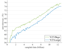
(a)

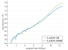
(b)

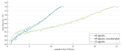
(c)

Figure 4: Training curves of scaling. The x-axis is the number of sampled data during training, and the y-axis is the zero-shot accuracy on IN-1K. The blue curve is the baseline setting: ViT-Large, LAION-400M data, 32 epochs (12.8B sampled data). In each subplot, we compare with scaling one factor on the baseline. In schedule scaling (Fig. LABEL:fig:scaling:length), we plot an extra hypothetical curve for a better visualization.

Image Captioning.

See Table 4.2 for the captioning performance on COCO [42] and nocaps [1]. Our captioning implementation follows the cross-entropy training baseline in [7]. Unlike classification in which only a classifier layer is added after pre-training, here the fine-tuning model has a newly initialized captioner (detailed in appendix). In this task, FLIP outperforms the original CLIP checkpoint in several metrics. Compared to our CLIP baseline, which is pre-trained on the same data, FLIP also shows a clear gain, especially in BLEU-4 and CIDEr metrics.

Visual Question Answering.

We evaluate on the VQAv2 dataset [26], with a fine-tuning setup following [21]. We use a newly initialized multimodal fusion transformer and an answer classifier to obtain the VQA outputs (detailed in appendix). Table 4.2 (rightmost column) reports results on VQAv2. All entries pre-trained on LAION perform similarly, and CLIP pre-trained on WIT is the best.

Summary of Comparisons.

Across a large variety of scenarios, FLIP is dominantly better than its CLIP counterparts (OpenCLIP and our reproduction) pre-trained on the same LAION data, in some cases by large margins.

The difference between the WIT data and LAION data can create large systematic gaps, as observed in many downstream tasks. We hope our study will draw attention to these data-dependent gaps in future research.

				zero-shot transfer					transfer learning
				zero-shot	text retrieval		image retrieval		lin-probe	fine-tune	captioning		vqa
case	model	data	sampled	IN-1K	Flickr30k	COCO	Flickr30k	COCO	IN-1K	IN-1K	COCO	nocaps	VQAv2
baseline	Large	400M	12.8B	74.3	88.4	59.8	75.0	44.1	83.6	86.9	127.7	85.9	74.7
model scaling	Huge	400M	12.8B	75.5	89.2	62.8	76.4	46.0	84.3	87.3	130.3	91.5	76.3
data scaling	Large	2B	12.8B	75.8	91.7	63.8	78.2	47.3	84.2	87.1	128.9	87.0	75.5
schedule scaling	Large	400M	25.6B	73.9	89.7	60.1	75.5	44.4	83.7	86.9	127.9	86.8	75.0
model+data scaling	Huge	2B	12.8B	77.6	92.8	67.0	79.9	49.5	85.1	87.7	130.4	92.6	77.1
joint scaling	Huge	2B	25.6B	78.8	93.1	67.8	80.9	50.5	85.6	87.9	130.2	91.2	77.3

Table 8: Scaling behavior of FLIP, evaluated on a diverse set of downstream tasks: classification, retrieval (R@1), captioning (CIDEr), and visual question answering. In the middle three rows, we scale along one of the three axes (model, data, schedule), and the green entries denote the best ones among these three scaling cases. Data scaling is in general favored under the zero-shot transfer scenario, while model scaling is in general favored under the transfer learning scenario (i.e., with trainable weights in downstream).

4.3 Scaling Behavior

Facilitated by the speed-up of FLIP, we explore the scaling behavior beyond the largest case studied in CLIP [52]. We study scaling along either of these three axes:

• Model scaling. We replace the ViT-L image encoder with ViT-H, which has $\scriptstyle\sim$2${\times}$ parameters. The text encoder is also scaled accordingly.

• Data scaling. We scale the pre-training data from 400 million to 2 billion, using the LAION-2B set [36]. To better separate the influence of more data from the influence of longer training, we fix the total number of sampled data (12.8B, which amounts to 32 epochs of 400M data and 6.4 epochs of 2B data).

• Schedule scaling. We increase the sampled data from 12.8B to 25.6B (64 epochs of 400M data).

We study scaling along one of these three axes at each time while keeping others unchanged. The results are summarized in Fig. 4 and Table 8.

Training curves.

The three scaling strategies exhibit different trends in training curves (Fig. 4).

Model scaling (Fig. LABEL:fig:scaling:model) presents a clear gap that persists throughout training, though the gap is smaller at the end.

Data scaling (Fig. LABEL:fig:scaling:data), on the other hand, performs similarly at the first half of training, but starts to present a good gain later. Note that there is no extra computational cost in this setting, as we control the total number of sampled data.

Schedule scaling (Fig. LABEL:fig:scaling:length) trains 2$\times$ longer. To provide a more intuitive comparison, we plot a hypothetical curve that is rescaled by 1/2 along the x-axis (dashed line). Despite the longer training, the gain is diminishing or none (more numbers in Table 8).

Transferability.

Table 8 provides an all-around comparison on various downstream tasks regarding the scaling behavior. Overall, model scaling and data scaling both can consistently outperform the baseline in all metrics, in some cases by large margins.

We categorize the downstream tasks into two scenarios: (i) zero-shot transfer, i.e., no learning is performed on the downstream dataset; (ii) transfer learning, i.e., part or all of the weights are trained on the downstream dataset. For the tasks studied here, data scaling is in general favored for zero-shot transfer, while model scaling is in general favored for transfer learning. However, it is worth noting that the transfer learning performance depends on the size of the downstream dataset, and training a big model on a too small downstream set is still subject to the overfitting risk.

It is encouraging to see that data scaling is clearly beneficial, even not incurring longer training nor additional computation. On the contrary, even spending more computation by schedule scaling gives diminishing returns. These comparisons suggest that large-scale data are beneficial mainly because they provide richer information.

Next we scale both model and data (Table 8, second last row). For all metrics, model+data scaling improves over scaling either alone. The gains of model scaling and data scaling are highly complementary: e.g., in zero-shot IN-1K, model scaling alone improves over the baseline by 1.2% (74.3%$\rightarrow$75.5%), and data scaling alone improves by 1.5% (74.3%$\rightarrow$75.8%). Scaling both improves by 3.3% (77.6%), more than the two deltas combined. This behavior is also observed in several other tasks. This indicates that a larger model desires more data to unleash its potential.

Finally, we report joint scaling all three axes (Table 8, last row). Our results show that combining schedule scaling leads to improved performances across most metrics. This suggests that schedule scaling is particularly beneficial when coupled with larger models and larger-scale data.

Our result of 78.8% on zero-shot IN-1K outperforms the state-of-the-art result trained on public data with ViT-H (78.0% of OpenCLIP). Also based on LAION-2B, their result is trained with 32B sampled data, 1.25$\times$ more than ours. Given the 50% masking we use, our training is estimated to be 2.5$\times$ faster than theirs if both were run on the same hardware. As OpenCLIP’s result reports a training cost of $\scriptstyle\sim$5,600 GPU-days, our method could save $\scriptstyle\sim$3,360 GPU-days based on a rough estimation. Additionally, without enabling 2$\times$ schedule, our entry of “model+data scaling” is estimated 5$\times$ faster than theirs and can save $\scriptstyle\sim$4,480 GPU-days. This is considerable cost reduction.

5 Discussion and Conclusion

Language is a stronger form of supervision than classical closed-set labels. Language provides rich information for supervision. Therefore, scaling, which can involve increasing capacity (model scaling) and increasing information (data scaling), is essential for attaining good results in language-supervised training.

CLIP [52] is an outstanding example of “simple algorithms that scale well”. The simple design of CLIP allows it to be relatively easily executed at substantially larger scales and achieve big leaps compared to preceding methods. Our method largely maintains the simplicity of CLIP while pushing it further along the scaling aspect.

Our method can provide a 2-3$\times$ speedup or more. For the scale concerned in this study, such a speedup can reduce wall-clock time by a great amount (e.g., at the order of thousands of TPU/GPU-days). Besides accelerating research cycles, the speedup can also save a great amount of energy and commercial cost. These are all ingredients of great importance in large-scale machine learning research.

Our study involves controlled comparisons with various CLIP baselines, which help us to break down the gaps contributed by different factors. We show that FLIP outperforms its CLIP counterparts pre-trained on the same LAION data. By comparing several LAION-based models and the original WIT-based ones, we observe that the pre-training data creates big systematic gaps in several tasks.

Our study provides controlled experiments on scaling behavior. We observe that data scaling is a favored scaling dimension, given that it can improve accuracy with no extra cost at training or inference time. Our fast method encourages us to scale beyond what is studied in this work.

Broader impacts.

Training large-scale models costs high energy consumption and carbon emissions. While our method has reduced such cost to 1/2-1/3, the remaining cost is still sizable. We hope our work will attract more attention to the research direction on reducing the cost of training vision-language models.

The numerical results in this paper are based on a publicly available large-scale dataset [56]. The resulting model weights will reflect the data biases, including potentially negative implications. When compared using the same data, the statistical differences between two methods should reflect the method properties to a good extent; however, when compared entries using different training data, the biases of the data should always be part of the considerations.

Appendix A Implementation Details

A.1 Pre-training

Encoders.

Table 9 shows the architecture we use. The design follows CLIP [52]. Our image encoder involves ViT-B, -L, -H [20], using the same patch size as in [20] (16 for B and L, 14 for H). We use global average pooling after the image encoder. The corresponding text encoder is of a smaller size, following [52]. We train ViT-B/-L with 256 TPU-v3 cores, and ViT-H with 512 cores. Table 9 also shows the model size of the image encoder, text encoder, and the entire model (including output projection layers).

Hyper-parameters.

Our default pre-training configuration is shown in Table 10. We use the linear learning rate scaling rule [24]: lr = base_lr$\times$batchsize / 256. We observe that using this rule allows us to change the batch size in ablations without extra learning rate search. The numerical precision we use is float32 by default. We also experimented with bfloat16, but only observed a $\scriptstyle\sim$1.1$\times$ speedup, which is consistent with the results reported in Google’s blog .

Unmasked tuning, which is a form of pre-training while disabling masking, follows Table 10, except that we lower the base learning rate to 4e-8 and shorten the warmup schedule to 25.6M samples.

A.2 ImageNet Classification

Zero-shot.

We follow the prompt engineering in [52]. Their code provides 80 templates. We use a subset of 7 templates they recommend; using all 80 templates gives similar results but is slower at inference.

Linear probing and fine-tuning.

The setting follows [29]. See Table 11 and Table 12.

A.3 Zero-shot Retrieval

We evaluate the performance of zero-shot retrieval on two standard benchmarks: Flickr30K [73] and COCO [42], respectively with 1K and 5K image-text pairs in their test sets. Following the protocol in CLIP [52], we extract the image and text embeddings from the corresponding encoders and perform retrieval based on the cosine similarities over candidate image-text pairs; no prompt is used.

A.4 Zero-shot Robustness Evaluation

In our zero-shot robustness evaluation on the ImageNet-related sets, we use the 7 prompts provided by [52], only except in IN-R we use all 80 prompts that are better than the 7 prompts by noticeable margins. The dataset preparation and split follow OpenCLIP [36].  In ObjectNet, we follow [52] to use the class names without prompts. In YTBB, we use the VOC prompts provided by [52].

	Embed	Vision Transformer			Text Transformer			# params (M)
Model	dim	layers	width	heads	layers	width	heads	vision	text	total
B/16	512	12	768	12	12	512	8	86	53	141
L/16	768	24	1024	16	12	768	12	303	109	414
H/14	1024	32	1280	16	24	1024	16	631	334	967

Table 9: Encoder specifics.

config	value
optimizer	AdamW [45]
base learning rate	4e-6
weight decay	0.2
optimizer momentum	$\beta_{1},\beta_{2}{=}0.9,0.95$ [10]
learning rate schedule	cosine decay [44]
warmup (in samples)	51.2M (B/L), 256M (H)
numerical precision	float32

Table 10: Pre-training setting.

config	value
optimizer	LARS [72]
base learning rate	0.01
weight decay	0
optimizer momentum	0.9
batch size	16384
learning rate schedule	cosine decay
warmup epochs	10
training epochs	90
augmentation	RandomResizedCrop

Table 11: Linear probing setting.

config	value
optimizer	AdamW
base learning rate	5e-5
weight decay	0.05
optimizer momentum	$\beta_{1},\beta_{2}{=}0.9,0.999$
layer-wise lr decay [14]	0.75
batch size	1024
learning rate schedule	cosine decay
warmup epochs	5
training epochs	50 (L/H)
augmentation	RandAug (9, 0.5) [15]
label smoothing [58]	0.1
mixup [76]	0.8
cutmix [75]	1.0
drop path [34]	0.2 (L/H)

Table 12: Fine-tuning setting.

A.5 More Zero-shot Datasets

For the experiments in Table 4.2, we use the prompts provided by [52]. We follow the data preparation scripts provided by [25] and [46] and load data using Tensorflow Datasets. Following [52], we report the mean accuracy per class for FGVC Aircraft, Oxford-IIIT Pets, Caltech-101, and Oxford Flowers 102 datasets; we report the mean of top-1 and top-5 accuracy for Kinetics-700, ROC AUC for Hateful Memes, and 11-point mAP for Pascal VOC 2007 Classification; we report top-1 accuracy for the rest of the datasets. We note that the Birdsnap dataset on Internet is shrinking over time and only 1850 test images are available for us (vs. 2149 images tested in [52], and 2443 originally).

A.6 Captioning

We build a sequence-to-sequence encoder-decoder transformer model on top of the ViT image encoder, with 3 encoder layers and 3 decoder layers following [7]. Specifically, the ViT image features are first linearly projected to a 384-dimensional sequence and further encoded by a 3-layer transformer encoder (of 384 width and 6 heads). For auto-regressive caption generation, we discard the pre-trained text encoder in FLIP and use a randomly initialized 3-layer transformer decoder (of 384 width and 6 heads) with cross-attention to encoder outputs. The model is trained to predict the next text token using the tokenizer in [52].

For simplicity, we supervise the image captioning model only with teacher forcing using a word-level cross-entropy loss [7]; we do not use the CIDEr score optimization in [7]. The full model is fine-tuned end-to-end with the AdamW optimizer, a batch size of 256, a learning rate of 1e-4 for newly added parameters, a weight decay of 1e-2, a warmup of 15% iterations, and a cosine decay learning rate schedule. The learning rate for the pre-trained ViT parameters is set to 1e-5 for ViT-L (and 5e-6 for ViT-H). The input image size is 512${\times}$512 for ViT-L/16 and 448${\times}$448 for ViT-H/14 (to keep the same sequence lengths).

All models are fine-tuned for image captioning on the COCO training split of [38] for 20 epochs. During inference, the image captions are predicted with auto-regressive decoding, and we report their performance on the COCO test split of [38] under different metrics.

To evaluate how the COCO-trained models generalize to novel objects, we evaluate these models directly on the nocaps [1] validation set, with no further fine-tuning.

A.7 Visual Question Answering

In our VQA experiments, we follow the architecture described in [21]. Specifically, the VQA task is casted as a classification problem over all answer classes. The input images are encoded by the ViT encoders. The input questions are encoded by a pre-trained RoBERTa text encoder [43], following the practice in [21]. A multimodal fusion Transformer (4 layers, 768-d, 12 heads, with merged attention [21]) is applied to combine the image and text representations. A two-layer MLP is applied on the class token of the fusion module to obtain the VQA output [21].

We fine-tune the VQA model end-to-end. The loss function is a binary sigmoid loss using soft scores [60]. We use a batch size of 256, a learning rate of 1e-4 for randomly initialized parameters, and a learning rate of 1e-5 (ViT-L) or 5e-6 (ViT-H) for the pre-trained ViT parameters. We use a weight decay of 1e-2, a warmup of 15% of iterations, and a cosine decay learning rate schedule. The input image size is 512${\times}$512 for ViT-L/16 and 448${\times}$448 for ViT-H/14.

All models are fine-tuned for 20 epochs on the VQAv2 train+val set, with additional question-answer pairs from Visual Genome [39], following [60]. We report results on the test-dev split from the evaluation server.

References

- [1] Harsh Agrawal, Karan Desai, Yufei Wang, Xinlei Chen, Rishabh Jain, Mark Johnson, Dhruv Batra, Devi Parikh, Stefan Lee, and Peter Anderson. Nocaps: Novel object captioning at scale. In ICCV, 2019.
- [2] Jean-Baptiste Alayrac, Jeff Donahue, Pauline Luc, Antoine Miech, Iain Barr, Yana Hasson, Karel Lenc, Arthur Mensch, Katie Millican, and Malcolm Reynolds. Flamingo: a visual language model for few-shot learning. arXiv:2204.14198, 2022.
- [3] Jimmy Lei Ba, Jamie Ryan Kiros, and Geoffrey E Hinton. Layer normalization. arXiv:1607.06450, 2016.
- [4] Alan Baade, Puyuan Peng, and David Harwath. MAE-AST: Masked autoencoding audio spectrogram transformer. arXiv:2203.16691, 2022.
- [5] Roman Bachmann, David Mizrahi, Andrei Atanov, and Amir Zamir. MultiMAE: Multi-modal multi-task masked autoencoders. arXiv:2204.01678, 2022.
- [6] Hangbo Bao, Li Dong, and Furu Wei. BEiT: BERT pre-training of image Transformers. arXiv:2106.08254, 2021.
- [7] Manuele Barraco, Marcella Cornia, Silvia Cascianelli, Lorenzo Baraldi, and Rita Cucchiara. The unreasonable effectiveness of clip features for image captioning: An experimental analysis. In CVPR, 2022.
- [8] James Bradbury, Roy Frostig, Peter Hawkins, Matthew James Johnson, Chris Leary, Dougal Maclaurin, George Necula, Adam Paszke, Jake VanderPlas, Skye Wanderman-Milne, and Qiao Zhang. JAX: composable transformations of Python+NumPy programs, 2018.
- [9] Hongxu Chen, Sixiao Zhang, and Guandong Xu. Graph masked autoencoder. arXiv:2202.08391, 2022.
- [10] Mark Chen, Alec Radford, Rewon Child, Jeffrey Wu, Heewoo Jun, David Luan, and Ilya Sutskever. Generative pretraining from pixels. In ICML, 2020.
- [11] Ting Chen, Simon Kornblith, Mohammad Norouzi, and Geoffrey Hinton. A simple framework for contrastive learning of visual representations. In ICML, 2020.
- [12] Tianqi Chen, Bing Xu, Chiyuan Zhang, and Carlos Guestrin. Training deep nets with sublinear memory cost. arXiv preprint arXiv:1604.06174, 2016.
- [13] Dading Chong, Helin Wang, Peilin Zhou, and Qingcheng Zeng. Masked spectrogram prediction for self-supervised audio pre-training. arXiv:2204.12768, 2022.
- [14] Kevin Clark, Minh-Thang Luong, Quoc V Le, and Christopher D Manning. ELECTRA: Pre-training text encoders as discriminators rather than generators. In ICLR, 2020.
- [15] Ekin D Cubuk, Barret Zoph, Jonathon Shlens, and Quoc V Le. Randaugment: Practical automated data augmentation with a reduced search space. In CVPR Workshops, 2020.
- [16] Jia Deng, Wei Dong, Richard Socher, Li-Jia Li, Kai Li, and Li Fei-Fei. ImageNet: A large-scale hierarchical image database. In CVPR, 2009.
- [17] Karan Desai and Justin Johnson. Virtex: Learning visual representations from textual annotations. In CVPR, 2021.
- [18] Jacob Devlin, Ming-Wei Chang, Kenton Lee, and Kristina Toutanova. BERT: Pre-training of deep bidirectional Transformers for language understanding. In NAACL, 2019.
- [19] Xiaoyi Dong, Yinglin Zheng, Jianmin Bao, Ting Zhang, Dongdong Chen, Hao Yang, Ming Zeng, Weiming Zhang, Lu Yuan, and Dong Chen. MaskCLIP: Masked self-distillation advances contrastive language-image pretraining. arXiv:2208.12262, 2022.
- [20] Alexey Dosovitskiy, Lucas Beyer, Alexander Kolesnikov, Dirk Weissenborn, Xiaohua Zhai, Thomas Unterthiner, Mostafa Dehghani, Matthias Minderer, Georg Heigold, Sylvain Gelly, Jakob Uszkoreit, and Neil Houlsby. An image is worth 16x16 words: Transformers for image recognition at scale. In ICLR, 2021.
- [21] Zi-Yi Dou, Yichong Xu, Zhe Gan, Jianfeng Wang, Shuohang Wang, Lijuan Wang, Chenguang Zhu, Pengchuan Zhang, Lu Yuan, Nanyun Peng, et al. An empirical study of training end-to-end vision-and-language transformers. In CVPR, 2022.
- [22] Christoph Feichtenhofer, Haoqi Fan, Yanghao Li, and Kaiming He. Masked Autoencoders as spatiotemporal learners. arXiv:2205.09113, 2022.
- [23] Xinyang Geng, Hao Liu, Lisa Lee, Dale Schuurams, Sergey Levine, and Pieter Abbeel. Multimodal Masked Autoencoders learn transferable representations. arXiv:2205.14204, 2022.
- [24] Priya Goyal, Piotr Dollár, Ross Girshick, Pieter Noordhuis, Lukasz Wesolowski, Aapo Kyrola, Andrew Tulloch, Yangqing Jia, and Kaiming He. Accurate, large minibatch SGD: Training ImageNet in 1 hour. arXiv:1706.02677, 2017.
- [25] Priya Goyal, Quentin Duval, Jeremy Reizenstein, Matthew Leavitt, Sum Min, Benjamin Lefaudeux, Mannat Singh, Vinicius Reis, Mathilde Caron, Piotr Bojanowski, Armand Joulin, and Ishan Misra. VISSL. https://github.com/facebookresearch/vissl, 2021.
- [26] Yash Goyal, Tejas Khot, Douglas Summers-Stay, Dhruv Batra, and Devi Parikh. Making the V in VQA matter: Elevating the role of image understanding in visual question answering. In CVPR, 2017.
- [27] Jean-Bastien Grill, Florian Strub, Florent Altché, Corentin Tallec, Pierre Richemond, Elena Buchatskaya, Carl Doersch, Bernardo Avila Pires, Zhaohan Guo, Mohammad Gheshlaghi Azar, Bilal Piot, Koray Kavukcuoglu, Remi Munos, and Michal Valko. Bootstrap your own latent - a new approach to self-supervised learning. In NeurIPS, 2020.
- [28] Raia Hadsell, Sumit Chopra, and Yann LeCun. Dimensionality reduction by learning an invariant mapping. In CVPR, 2006.
- [29] Kaiming He, Xinlei Chen, Saining Xie, Yanghao Li, Piotr Dollár, and Ross Girshick. Masked autoencoders are scalable vision learners. arXiv:2111.06377, 2021.
- [30] Kaiming He, Haoqi Fan, Yuxin Wu, Saining Xie, and Ross Girshick. Momentum contrast for unsupervised visual representation learning. In CVPR, 2020.
- [31] Sunan He, Taian Guo, Tao Dai, Ruizhi Qiao, Chen Wu, Xiujun Shu, and Bo Ren. VLMAE: Vision-language masked autoencoder. arXiv:2208.09374, 2022.
- [32] Zhenyu Hou, Xiao Liu, Yuxiao Dong, Chunjie Wang, and Jie Tang. GraphMAE: Self-supervised masked graph autoencoders. arXiv:2205.10803, 2022.
- [33] Zejiang Hou, Fei Sun, Yen-Kuang Chen, Yuan Xie, and Sun-Yuan Kung. MILAN: Masked image pretraining on language assisted representation. arXiv:2208.06049, 2022.
- [34] Gao Huang, Yu Sun, Zhuang Liu, Daniel Sedra, and Kilian Q Weinberger. Deep networks with stochastic depth. In ECCV, 2016.
- [35] Po-Yao Huang, Hu Xu, Juncheng Li, Alexei Baevski, Michael Auli, Wojciech Galuba, Florian Metze, and Christoph Feichtenhofer. Masked autoencoders that listen. arXiv:2207.06405, 2022.
- [36] Gabriel Ilharco, Mitchell Wortsman, Ross Wightman, Cade Gordon, Nicholas Carlini, Rohan Taori, Achal Dave, Vaishaal Shankar, Hongseok Namkoong, John Miller, Hannaneh Hajishirzi, Ali Farhadi, and Ludwig Schmidt. OpenCLIP, 2021.
- [37] Chao Jia, Yinfei Yang, Ye Xia, Yi-Ting Chen, Zarana Parekh, Hieu Pham, Quoc Le, Yun-Hsuan Sung, Zhen Li, and Tom Duerig. Scaling up visual and vision-language representation learning with noisy text supervision. In ICML, 2021.
- [38] Andrej Karpathy and Li Fei-Fei. Deep visual-semantic alignments for generating image descriptions. In CVPR, 2015.
- [39] Ranjay Krishna, Yuke Zhu, Oliver Groth, Justin Johnson, Kenji Hata, Joshua Kravitz, Stephanie Chen, Yannis Kalantidis, Li-Jia Li, David A Shamma, et al. Visual genome: Connecting language and vision using crowdsourced dense image annotations. International journal of computer vision, 123(1):32–73, 2017.
- [40] Alex Krizhevsky, Ilya Sutskever, and Geoff Hinton. Imagenet classification with deep convolutional neural networks. In NeurIPS, 2012.
- [41] Gukyeong Kwon, Zhaowei Cai, Avinash Ravichandran, Erhan Bas, Rahul Bhotika, and Stefano Soatto. Masked vision and language modeling for multi-modal representation learning. arXiv:2208.02131, 2022.
- [42] Tsung-Yi Lin, Michael Maire, Serge Belongie, James Hays, Pietro Perona, Deva Ramanan, Piotr Dollár, and C Lawrence Zitnick. Microsoft COCO: Common objects in context. In ECCV, 2014.
- [43] Yinhan Liu, Myle Ott, Naman Goyal, Jingfei Du, Mandar Joshi, Danqi Chen, Omer Levy, Mike Lewis, Luke Zettlemoyer, and Veselin Stoyanov. RoBERTa: A robustly optimized BERT pretraining approach. arXiv preprint arXiv:1907.11692, 2019.
- [44] Ilya Loshchilov and Frank Hutter. SGDR: Stochastic gradient descent with warm restarts. In ICLR, 2017.
- [45] Ilya Loshchilov and Frank Hutter. Decoupled weight decay regularization. In ICLR, 2019.
- [46] Norman Mu, Alexander Kirillov, David Wagner, and Saining Tie. SLIP: Self-supervision meets language-image pre-training. In ECCV, 2022.
- [47] Daisuke Niizumi, Daiki Takeuchi, Yasunori Ohishi, Noboru Harada, and Kunio Kashino. Masked spectrogram modeling using masked autoencoders for learning general-purpose audio representation. arXiv:2204.12260, 2022.
- [48] Aaron van den Oord, Yazhe Li, and Oriol Vinyals. Representation learning with contrastive predictive coding. arXiv:1807.03748, 2018.
- [49] Yatian Pang, Wenxiao Wang, Francis EH Tay, Wei Liu, Yonghong Tian, and Li Yuan. Masked autoencoders for point cloud self-supervised learning. arXiv:2203.06604, 2022.
- [50] Deepak Pathak, Philipp Krahenbuhl, Jeff Donahue, Trevor Darrell, and Alexei A Efros. Context encoders: Feature learning by inpainting. In CVPR, 2016.
- [51] Hieu Pham, Zihang Dai, Golnaz Ghiasi, Hanxiao Liu, Adams Wei Yu, Minh-Thang Luong, Mingxing Tan, and Quoc V Le. Combined scaling for zero-shot transfer learning. arXiv:2111.10050, 2021.
- [52] Alec Radford, Jong Wook Kim, Chris Hallacy, Aditya Ramesh, Gabriel Goh, Sandhini Agarwal, Girish Sastry, Amanda Askell, Pamela Mishkin, Jack Clark, Gretchen Krueger, and Ilya Sutskever. Learning transferable visual models from natural language supervision. In ICML, 2021.
- [53] Aditya Ramesh, Prafulla Dhariwal, Alex Nichol, Casey Chu, and Mark Chen. Hierarchical text-conditional image generation with clip latents. arXiv:2204.06125, 2022.
- [54] Adam Roberts, Hyung Won Chung, Anselm Levskaya, Gaurav Mishra, James Bradbury, Daniel Andor, Sharan Narang, Brian Lester, Colin Gaffney, Afroz Mohiuddin, Curtis Hawthorne, Aitor Lewkowycz, Alex Salcianu, Marc van Zee, Jacob Austin, Sebastian Goodman, Livio Baldini Soares, Haitang Hu, Sasha Tsvyashchenko, Aakanksha Chowdhery, Jasmijn Bastings, Jannis Bulian, Xavier Garcia, Jianmo Ni, Andrew Chen, Kathleen Kenealy, Jonathan H. Clark, Stephan Lee, Dan Garrette, James Lee-Thorp, Colin Raffel, Noam Shazeer, Marvin Ritter, Maarten Bosma, Alexandre Passos, Jeremy Maitin-Shepard, Noah Fiedel, Mark Omernick, Brennan Saeta, Ryan Sepassi, Alexander Spiridonov, Joshua Newlan, and Andrea Gesmundo. Scaling up models and data with t5x and seqio. arXiv:2203.17189, 2022.
- [55] Robin Rombach, Andreas Blattmann, Dominik Lorenz, Patrick Esser, and Björn Ommer. High-resolution image synthesis with latent diffusion models. In CVPR, 2022.
- [56] Christoph Schuhmann, Romain Beaumont, Richard Vencu, Cade Gordon, Ross Wightman, Mehdi Cherti, Theo Coombes, Aarush Katta, Clayton Mullis, Mitchell Wortsman, Patrick Schramowski, Srivatsa Kundurthy, Katherine Crowson, Ludwig Schmidt, Robert Kaczmarczyk, and Jenia Jitsev. LAION-5B: An open large-scale dataset for training next generation image-text models. In NeurIPS, 2022.
- [57] Younggyo Seo, Danijar Hafner, Hao Liu, Fangchen Liu, Stephen James, Kimin Lee, and Pieter Abbeel. Masked world models for visual control. arXiv:2206.14244, 2022.
- [58] Christian Szegedy, Vincent Vanhoucke, Sergey Ioffe, Jonathon Shlens, and Zbigniew Wojna. Rethinking the inception architecture for computer vision. In CVPR, 2016.
- [59] Qiaoyu Tan, Ninghao Liu, Xiao Huang, Rui Chen, Soo-Hyun Choi, and Xia Hu. MGAE: Masked autoencoders for self-supervised learning on graphs. arXiv:2201.02534, 2022.
- [60] Damien Teney, Peter Anderson, Xiaodong He, and Anton Van Den Hengel. Tips and tricks for visual question answering: Learnings from the 2017 challenge. In CVPR, 2018.
- [61] Zhan Tong, Yibing Song, Jue Wang, and Limin Wang. VideoMAE: Masked autoencoders are data-efficient learners for self-supervised video pre-training. arXiv:2203.12602, 2022.
- [62] Ashish Vaswani, Noam Shazeer, Niki Parmar, Jakob Uszkoreit, Llion Jones, Aidan N Gomez, Lukasz Kaiser, and Illia Polosukhin. Attention is all you need. In NeurIPS, 2017.
- [63] Pascal Vincent, Hugo Larochelle, Yoshua Bengio, and Pierre-Antoine Manzagol. Extracting and composing robust features with denoising autoencoders. In ICML, 2008.
- [64] Pascal Vincent, Hugo Larochelle, Isabelle Lajoie, Yoshua Bengio, Pierre-Antoine Manzagol, and Léon Bottou. Stacked denoising autoencoders: Learning useful representations in a deep network with a local denoising criterion. JMLR, 2010.
- [65] Zirui Wang, Jiahui Yu, Adams Wei Yu, Zihang Dai, Yulia Tsvetkov, and Yuan Cao. SimVLM: Simple visual language model pretraining with weak supervision. arXiv:2108.10904, 2021.
- [66] Chen Wei, Haoqi Fan, Saining Xie, Chao-Yuan Wu, Alan Yuille, and Christoph Feichtenhofer. Masked feature prediction for self-supervised visual pre-training. arXiv:2112.09133, 2021.
- [67] Yixuan Wei, Han Hu, Zhenda Xie, Zheng Zhang, Yue Cao, Jianmin Bao, Dong Chen, and Baining Guo. Contrastive learning rivals masked image modeling in fine-tuning via feature distillation. arXiv:2205.14141, 2022.
- [68] Mitchell Wortsman, Gabriel Ilharco, Jong Wook Kim, Mike Li, Simon Kornblith, Rebecca Roelofs, Raphael Gontijo Lopes, Hannaneh Hajishirzi, Ali Farhadi, Hongseok Namkoong, et al. Robust fine-tuning of zero-shot models. In CVPR, 2022.
- [69] Zhirong Wu, Zihang Lai, Xiao Sun, and Stephen Lin. Extreme masking for learning instance and distributed visual representations. arXiv:2206.04667, 2022.
- [70] Tete Xiao, Ilija Radosavovic, Trevor Darrell, and Jitendra Malik. Masked visual pre-training for motor control. arXiv:2203.06173, 2022.
- [71] Zhenda Xie, Zheng Zhang, Yue Cao, Yutong Lin, Jianmin Bao, Zhuliang Yao, Qi Dai, and Han Hu. SimMIM: A simple framework for masked image modeling. arXiv:2111.09886, 2021.
- [72] Yang You, Igor Gitman, and Boris Ginsburg. Large batch training of convolutional networks. arXiv:1708.03888, 2017.
- [73] Peter Young, Alice Lai, Micah Hodosh, and Julia Hockenmaier. From image descriptions to visual denotations: New similarity metrics for semantic inference over event descriptions. Transactions of the Association for Computational Linguistics, 2014.
- [74] Jiahui Yu, Zirui Wang, Vijay Vasudevan, Legg Yeung, Mojtaba Seyedhosseini, and Yonghui Wu. CoCa: Contrastive captioners are image-text foundation models. arXiv:2205.01917, 2022.
- [75] Sangdoo Yun, Dongyoon Han, Seong Joon Oh, Sanghyuk Chun, Junsuk Choe, and Youngjoon Yoo. Cutmix: Regularization strategy to train strong classifiers with localizable features. In ICCV, 2019.
- [76] Hongyi Zhang, Moustapha Cisse, Yann N Dauphin, and David Lopez-Paz. mixup: Beyond empirical risk minimization. In ICLR, 2018.