SMEFT truncation effects in Higgs boson pair production at NLO QCD

Abstract

We present results for Higgs boson pair production in gluon fusion at next-to-leading order in QCD, including effects of anomalous couplings within Standard Model Effective Field Theory (SMEFT). In particular, we investigate truncation effects of the SMEFT series, comparing different ways to treat powers of dimension-six operators and double operator insertions.

1 Introduction

Higgs boson pair production in gluon fusion offers the possibility to measure the trilinear Higgs boson self-coupling and therefore to verify whether the form of the Higgs potential assumed in the Standard Model (SM) is correct. Deviations from this form, manifesting themselves in anomalous Higgs boson self-couplings, would be a clear sign of new physics and most likely would come along with other non-SM Higgs couplings. Therefore it is important to control the uncertainties of the theory predictions in simulations that include anomalous couplings. The theoretical uncertainties have various sources, the dominant ones in the SM being uncertainties related to the top quark mass renormalisation scheme. Theory predictions with full top quark mass dependence are available at NLO QCD [1, 2, 3, 4] and have been included in calculations where higher orders have been performed in the heavy top limit [5, 6, 7], thus reducing the scale uncertainties and the uncertainties due to missing top quark mass effects, such that the top mass scheme uncertainties currently constitute the main uncertainties [8] of the SM predictions.

Going beyond the SM description of the process $gg\to HH$, considering in particular effective field theory (EFT) parametrisations of new physics effects, new uncertainties arise, coming mainly from the truncation of the EFT expansion.

In the following we will present results at NLO SMEFT for this process, including also double operator insertions. Our implementation allows us to investigate various scenarios of truncation and to assess the related uncertainties. For more details we refer to Ref. [9].

2 Effective field theory descriptions of Higgs boson pair production

2.1 HEFT and SMEFT

In Standard Model Effective Field Theory (SMEFT) [10, 11], an effective description of unknown interactions at a new physics scale $\Lambda$ is constructed as an expansion in inverse powers of $\Lambda$, with operators $\mathcal{O}_{i}$ of canonical dimension larger than four and corresponding Wilson coefficients $C_{i}$,

$$\mathcal{L}_{\text{SMEFT}}=\mathcal{L}_{\text{SM}}+\sum_{i}\frac{C_{i}^{(6)}}{\Lambda^{2}}\mathcal{O}_{i}^{\rm{dim6}}+{\cal O}(\frac{1}{\Lambda^{3}})\;.$$ (1)

In SMEFT it is assumed that the physical Higgs boson is part of a doublet transforming linearly under $SU(2)_{L}\times U(1)$.

Higgs Effective Field Theory (HEFT) instead is based on an expansion in terms of loop orders, which also can be formulated in terms of chiral dimension counting [12, 13]. The expansion parameter is given by $f^{2}/\Lambda^{2}\simeq\frac{1}{16\pi^{2}}$, where $f$ is a typical energy scale at which the EFT expansion is valid (for example the pion decay constant in chiral perturbation theory),

$${\cal L}_{d_{\chi}}={\cal L}_{(d_{\chi}=2)}+\sum_{L=1}^{\infty}\sum_{i}\left(\frac{1}{16\pi^{2}}\right)^{L}c_{i}^{(L)}O^{(L)}_{i}\;.$$ (2)

The SMEFT Lagrangian is typically given in the so-called Warsaw basis [10], the terms relevant to the process $gg\to HH$ read

$$\begin{split}\Delta\mathcal{L}_{\text{Warsaw}}&=\frac{C_{H,\Box}}{\Lambda^{2}}(\phi^{\dagger}\phi)\Box(\phi^{\dagger}\phi)+\frac{C_{HD}}{\Lambda^{2}}(\phi^{\dagger}D_{\mu}\phi)^{*}(\phi^{\dagger}D^{\mu}\phi)+\frac{C_{H}}{\Lambda^{2}}(\phi^{\dagger}\phi)^{3}\\ &+\left(\frac{C_{uH}}{\Lambda^{2}}\phi^{\dagger}{\phi}\bar{q}_{L}\phi^{c}t_{R}+h.c.\right)+\frac{C_{HG}}{\Lambda^{2}}\phi^{\dagger}\phi G_{\mu\nu}^{a}G^{\mu\nu,a}\;.\end{split}$$ (3)

The dipole operator $\bar{{\cal O}}_{uG}$ is not included here because it can be shown that it carries an extra loop suppression factor $1/16\pi^{2}$ relative to the other contributions if weak coupling to the heavy sector is assumed [14, 15]. In the strong coupling case an expansion in the canonical dimension only would not be the appropriate description.

The HEFT Lagrangian relevant to Higgs boson pair production in gluon fusion can be parametrised by five a priori independent anomalous couplings as follows [14]

$$\Delta{\cal L}_{\text{HEFT}}=-m_{t}\left(c_{t}\frac{h}{v}+c_{tt}\frac{h^{2}}{v^{2}}\right)\,\bar{t}\,t-c_{hhh}\frac{m_{h}^{2}}{2v}h^{3}+\frac{\alpha_{s}}{8\pi}\left(c_{ggh}\frac{h}{v}+c_{gghh}\frac{h^{2}}{v^{2}}\right)\,G^{a}_{\mu\nu}G^{a,\mu\nu}\;.$$ (4)

Expanding the Higgs doublet in eq. (3) around its vacuum expectation value and applying a field redefinition for the physical Higgs boson

$$h\to h+v^{2}\frac{C_{H,kin}}{\Lambda^{2}}\left(h+h^{2}+\frac{h^{3}}{3}\right)\;,$$ (5)

with $\frac{C_{H,kin}}{\Lambda^{2}}:=\frac{C_{H,\Box}}{\Lambda^{2}}-\frac{1}{4}\frac{C_{HD}}{\Lambda^{2}}$, the Higgs kinetic term acquires its canonical form (up to ${\cal O}\left(\Lambda^{-4}\right)$ terms). After that, relating the couplings through a comparison of the coefficients of the corresponding terms in the Lagrangian leads to the expressions given in Table 1.

HEFT	Warsaw
$c_{hhh}$	$1-2\frac{v^{2}}{\Lambda^{2}}\frac{v^{2}}{m_{h}^{2}}\,C_{H}+3\frac{v^{2}}{\Lambda^{2}}\,C_{H,kin}$
$c_{t}$	$1+\frac{v^{2}}{\Lambda^{2}}\,C_{H,kin}-\frac{v^{2}}{\Lambda^{2}}\frac{v}{\sqrt{2}m_{t}}\,C_{uH}$
$c_{tt}$	$-\frac{v^{2}}{\Lambda^{2}}\frac{3v}{2\sqrt{2}m_{t}}\,C_{uH}+\frac{v^{2}}{\Lambda^{2}}\,C_{H,kin}$
$c_{ggh}$	$\frac{v^{2}}{\Lambda^{2}}\frac{8\pi}{\alpha_{s}}\,C_{HG}$
$c_{gghh}$	$\frac{v^{2}}{\Lambda^{2}}\frac{4\pi}{\alpha_{s}}\,C_{HG}$

Table 1: Leading order translation between different operator basis choices.

However, it should be emphasized that a translation between the coefficients at Lagrangian level must be applied with care. The EFT parametrisations have a validity range limited by unitarity constraints and the assumption that $C_{i}/\Lambda^{2}$ in SMEFT is a small quantity. Furthermore there are relations between the coefficients in SMEFT which are not present in HEFT. Therefore a naive translation from HEFT (which is more general) to SMEFT can lead out of the validity range for a given point in the coupling parameter space, even if it is a perfectly valid point in HEFT.

2.2 SMEFT truncation

Another delicate point in the EFT expansion is the question how to treat terms with inverse powers of $\Lambda$ higher than two at cross section level, i.e. when squaring the amplitude. These are terms related to squared dim-6 operators, double operator insertions in a single diagram and combinations thereof. Related issues have been discussed recently in Ref. [16].

We now present a Monte Carlo program which allows us to study the truncation effects systematically. In order to construct the different truncation options we first deconstruct the amplitude into three parts: the pure SM contribution (SM), single dim-6 operator insertions ($\rm{dim6}$) and double dim-6 operator insertions ($\rm{dim6}^{2}$):

$${\cal M}= \ \begin{aligned} \vbox{\hbox{\includegraphics[page=8,scale={0.7}]{figures/HH_presentation}}}\\[-6.0pt] \scalebox{0.1}{{\color[rgb]{1,1,1}dummy}}\end{aligned}+\vbox{\hbox{\includegraphics[page=9,scale={0.7}]{figures/HH_presentation}}}+\vbox{\hbox{\includegraphics[page=10,scale={0.7}]{figures/HH_presentation}}}$$

$$\ +\vbox{\hbox{\includegraphics[page=11,scale={0.7}]{figures/HH_presentation}}}+\vbox{\hbox{\includegraphics[page=12,scale={0.7}]{figures/HH_presentation}}}+\dots$$

$$= \ {\cal M}_{\text{SM}}+{\cal M}_{\rm{dim6}}+{\cal M}_{\rm{dim6}^{2}}\;,$$ (6)

where $c^{\prime}$ denotes the corresponding coupling combination listed in Table 1. For the squared amplitude forming the cross section, we consider four possibilities to choose which parts of $|{\cal M}|^{2}$ from eq. (6) may enter:

$$\sigma\simeq\left\{\begin{aligned} &\ \sigma_{\text{SM}}+\sigma_{\text{SM}\times\rm{dim6}}\\ &\ \sigma_{\left(\text{SM}+\rm{dim6}\right)\times\left(\text{SM}+\rm{dim6}\right)}\\ &\ \sigma_{\left(\text{SM}+\rm{dim6}\right)\times\left(\text{SM}+\rm{dim6}\right)}+\sigma_{\text{SM}\times\rm{dim6}^{2}}\\ &\ \sigma_{\left(\text{SM}+\rm{dim6}+\rm{dim6}^{2}\right)\times\left(\text{SM}+\rm{dim6}+\rm{dim6}^{2}\right)}\;.\end{aligned}\right.$$ (7)

The first line is the first order of an expansion of $\sigma\sim|{\cal M}|^{2}$ in $\Lambda^{-2}$, the second term is the first order of an expansion of ${\cal M}$ in $\Lambda^{-2}$. The third line includes all terms of ${\cal O}\left(\Lambda^{-4}\right)$ coming from single and double dim-6 operator insertions, however it lacks the contribution at the same order from dim-8 operators and ${\cal O}\left(\Lambda^{-4}\right)$ terms following the field redefinition of eq. (5). The fourth line is the naive translation from HEFT to SMEFT using Table 1. Typically, only the first two options are used for predictions and measurements using SMEFT, since both are unambiguous wrt. basis change and gauge invariance, however there is still a debate about the recommendations for their application to experimental analyses [16]. Thus, we include all of the presented options in our calculation, which can serve to contrast different outcomes of the predictions.

3 NLO Implementation into the event generator program POWHEG and results

3.1 Parametrisation of the $gg\to HH$ total cross section

Our implementation is based on the publicly available NLO HEFT code presented in Refs. [17, 18], converted to the SMEFT framework and extended such that the different options described in the previous section can be calculated, including NLO QCD corrections.

For the real emission, a modified GoSam [19] version is built that splits the amplitude evaluation according to eq. (6) and is able to generate the squared amplitude with the truncation option which can be set by the user via an input variable. For the generation of the GoSam files in POWHEG [20], a model in UFO format [21] has been produced which specifies the anomalous couplings such that GoSam is able to calculate the different contributions according to the chosen truncation option. The existing interface to POWHEG has been modified to hand over event parameters to GoSam such that the factor $\alpha_{s}$ between Higgs-gluon couplings in HEFT and SMEFT is evaluated at the correct energy scale.

The virtual part is based on grids encoding the virtual 2-loop amplitudes. These grids can be used to reconstruct the amplitude for any given combination of anomalous couplings. The $a_{i}$ listed below are defined as the coefficients in the representation of the sqared amplitude as a linear combination of all coupling combinations possible in HEFT at NLO QCD.

$$|{\cal M}_{BSM}|^{2}= a_{1}\cdot c_{t}^{4}+a_{2}\cdot c_{tt}^{2}+a_{3}\cdot c_{t}^{2}c_{hhh}^{2}+a_{4}\cdot c_{ggh}^{2}c_{hhh}^{2}+a_{5}\cdot c_{gghh}^{2}+a_{6}\cdot c_{tt}c_{t}^{2}+a_{7}\cdot c_{t}^{3}c_{hhh}$$

$$+ a_{8}\cdot c_{tt}c_{t}c_{hhh}+a_{9}\cdot c_{tt}c_{ggh}c_{hhh}+a_{10}\cdot c_{tt}c_{gghh}+a_{11}\cdot c_{t}^{2}c_{ggh}c_{hhh}+a_{12}\cdot c_{t}^{2}c_{gghh}$$

$$+ a_{13}\cdot c_{t}c_{hhh}^{2}c_{ggh}+a_{14}\cdot c_{t}c_{hhh}c_{gghh}+a_{15}\cdot c_{ggh}c_{hhh}c_{gghh}+a_{16}\cdot c_{t}^{3}c_{ggh}$$

$$+ a_{17}\cdot c_{t}c_{tt}c_{ggh}+a_{18}\cdot c_{t}c_{ggh}^{2}c_{hhh}+a_{19}\cdot c_{t}c_{ggh}c_{gghh}+a_{20}\cdot c_{t}^{2}c_{ggh}^{2}$$

$$+ a_{21}\cdot c_{tt}c_{ggh}^{2}+a_{22}\cdot c_{ggh}^{3}c_{hhh}+a_{23}\cdot c_{ggh}^{2}c_{gghh}\;.$$

Since the first and the third truncation options of eq. (7) are expansions at cross section level, and the fourth option is the direct translation from HEFT to SMEFT, for those cases the application of the translation of Table 1, including all terms at the desired order in inverse $\Lambda$, is sufficient. In the case of the second truncation option, some of the grids can be reused as well, but the determination of the coefficients needs more care, as there are additional combinations. Note that we do not include RGE running of the couplings as we only consider NLO QCD corrections to the amplitude, which factorise.

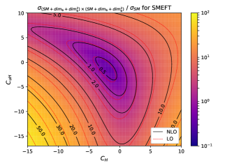
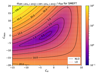
Figure 1: Heat maps showing the dependence of the cross section on the couplings $C_{H}$, $C_{uH}$ (left) and $C_{H}$, $C_{H,kin}$ (right) with $\Lambda=1$ TeV for different truncation options. Top: option 1 (linear dim-6), bottom: option 2 (quadratic dim-6). The white areas denote regions in parameter space where the corresponding cross section would be negative.

In Fig. 1 we show that the results for the total cross sections (normalised to the SM case) are substantially different between option 1 (linear dim-6, top) and option 2 (quadratic dim-6, bottom). The white areas come from the fact that taking into account only linear dim6-contributions leads to negative cross sections over large parts of the parameter space. Furthermore, in the linear dim-6 case, there appears to be a completely flat direction in the observed parameter range for a combined variation of the respective Wilson coefficients in the diagrams. Flat directions are apparent in option 2 as well, however they correspond to an elliptic shape of equipotential lines due to the quadratic terms in the cross section.

3.2 Investigation of truncation effects for the Higgs boson pair invariant mass distribution

Now we turn to differential results, showing the effects of the different truncation options on the Higgs boson pair invariant mass distribution $m_{hh}$. We present results at two benchmark points, given in Table 2, which were derived analogously to [22] based on an analysis of characteristic shapes of the $m_{hh}$ distribution, but with the inclusion of current experimental constraints. The upper panels show results for $\Lambda=1$ TeV, the lower panels show results for the same point for $\Lambda=2$ TeV, for the different truncation options. One can clearly see that (a) the negative differential cross section values in the linear dim-6 case (blue) indicate that parameter points in anomalous coupling parameter space which are valid in HEFT can lead, upon naive translation, to parameter points for which the SMEFT expansion is not valid, (b) destructive interference between different parts of the amplitude (e.g. box- and triangle-type diagams) can be enhanced or diminished depending on the truncation option, (c) increasing $\Lambda$ reduces the differences between the results as they are smaller deformations of the SM parameter space. In addition, we observe that the contribution from the interference of double dim-6 operator insertions with the SM appears to be subdominant in the example of benchmark point $1^{\ast}$, as can be seen by comparing truncation option 2 (orange) with option 3 (red), the latter including the double operator insertions. We also should point out that the difference between HEFT (cyan) and SMEFT with truncation option 4 (green) is due to the scale dependence of $\alpha_{s}$, coming from the definition of $C_{HG}$ in the Warsaw basis, see Table 1.

benchmark (${}^{\ast}=$ modified)	$c_{hhh}$	$c_{t}$	$c_{tt}$	$c_{ggh}$	$c_{gghh}$	$C_{H,\textrm{kin}}$	$C_{H}$	$C_{uH}$	$C_{HG}$	$\Lambda$
SM	$1$	$1$	$0$	$0$	$0$	$0$	$0$	$0$	$0$	$1\;$TeV
$1^{\ast}$	$5.105$	$1.1$	$0$	$0$	$0$	$4.95$	$-6.81$	$3.28$	$0$	$1\;$TeV
$6^{\ast}$	$-0.684$	$0.9$	$-\frac{1}{6}$	$0.5$	$0.25$	$0.561$	$3.80$	$2.20$	$0.0387$	$1\;$TeV

Table 2: Benchmark points used for the invariant mass distributions. The benchmark points were derived analogously to [22], but are slightly modified compared to the ones given in [22], to take into account current experimental constraints. The value of $C_{HG}$ is determined using $\alpha_{s}(m_{Z})=0.118$.

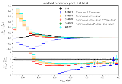
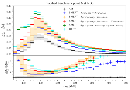
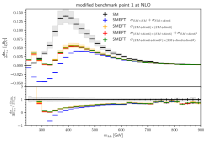
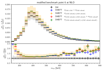
Figure 2: Differential cross sections for the Higgs boson pair invariant mass. Top row: $\Lambda=1$ TeV, bottom row: $\Lambda=2$ TeV. Left: benchmark point $1^{\ast}$, right: benchmark point $6^{\ast}$ of Table 2. The gray and orange bands show the uncertainty from 3-point scale variations $\mu_{R}=\mu_{F}=c\cdot m_{hh}/2$, with $c\in\{\frac{1}{2},1,2\}$, for the SM and SMEFT $\sigma_{(SM+dim6)\times(SM+dim6)}$, respectively.

4 Summary

We have presented NLO QCD corrections to Higgs boson pair production in combination with a Standard Model Effective Field Theory (SMEFT) parametrisation of effects of physics beyond the Standard Model. The calculation has been implemented into the GoSam+POWHEG Monte Carlo program framework in a way which allows to choose different options for the truncation of the EFT series and to compare to results in (non-linear) Higgs Effective Field Theory (HEFT). The results show that a naive translation between HEFT and SMEFT has pitfalls and that the various truncation options can lead to large differences in the theory predictions.

Acknowledgements

We would like to thank Stephen Jones, Matthias Kerner and Ludovic Scyboz for collaboration in the $ggHH$@NLO project and Gerhard Buchalla for useful discussions. Special thanks to Ludovic for providing up-to-date benchmark points. This research was supported by the Deutsche Forschungsgemeinschaft (DFG, German Research Foundation) under grant 396021762 - TRR 257.

References

References

- [1] Borowka S, Greiner N, Heinrich G, Jones S P, Kerner M, Schlenk J, Schubert U and Zirke T 2016 Phys. Rev. Lett. 117 012001 [Erratum: Phys.Rev.Lett. 117, 079901 (2016)] (Preprint 1604.06447)
- [2] Borowka S, Greiner N, Heinrich G, Jones S P, Kerner M, Schlenk J and Zirke T 2016 JHEP 10 107 (Preprint 1608.04798)
- [3] Baglio J, Campanario F, Glaus S, Mühlleitner M, Spira M and Streicher J 2019 Eur. Phys. J. C 79 459 (Preprint 1811.05692)
- [4] Baglio J, Campanario F, Glaus S, Mühlleitner M, Ronca J, Spira M and Streicher J 2020 JHEP 04 181 (Preprint 2003.03227)
- [5] Grazzini M, Heinrich G, Jones S, Kallweit S, Kerner M, Lindert J M and Mazzitelli J 2018 JHEP 05 059 (Preprint 1803.02463)
- [6] Chen L B, Li H T, Shao H S and Wang J 2020 Phys. Lett. B 803 135292 (Preprint 1909.06808)
- [7] Chen L B, Li H T, Shao H S and Wang J 2020 JHEP 03 072 (Preprint 1912.13001)
- [8] Baglio J, Campanario F, Glaus S, Mühlleitner M, Ronca J and Spira M 2021 Phys. Rev. D 103 056002 (Preprint 2008.11626)
- [9] Heinrich G, Lang J and Scyboz L 2022 JHEP 08 079 (Preprint 2204.13045)
- [10] Grzadkowski B, Iskrzynski M, Misiak M and Rosiek J 2010 JHEP 10 085 (Preprint 1008.4884)
- [11] Brivio I and Trott M 2019 Phys. Rept. 793 1–98 (Preprint 1706.08945)
- [12] Buchalla G, Catá O and Krause C 2014 Phys. Lett. B 731 80–86 (Preprint 1312.5624)
- [13] Krause C G 2016 Higgs Effective Field Theories - Systematics and Applications Ph.D. thesis Munich U. (Preprint 1610.08537)
- [14] Buchalla G, Capozi M, Celis A, Heinrich G and Scyboz L 2018 JHEP 09 057 (Preprint 1806.05162)
- [15] Arzt C, Einhorn M B and Wudka J 1995 Nucl. Phys. B 433 41–66 (Preprint hep-ph/9405214)
- [16] Brivio I et al. 2022 (Preprint 2201.04974)
- [17] Heinrich G, Jones S P, Kerner M, Luisoni G and Scyboz L 2019 JHEP 06 066 (Preprint 1903.08137)
- [18] Heinrich G, Jones S P, Kerner M and Scyboz L 2020 JHEP 10 021 (Preprint 2006.16877)
- [19] Cullen G et al. 2014 Eur. Phys. J. C 74 3001 (Preprint 1404.7096)
- [20] Alioli S, Nason P, Oleari C and Re E 2010 JHEP 06 043 (Preprint 1002.2581)
- [21] Degrande C, Duhr C, Fuks B, Grellscheid D, Mattelaer O and Reiter T 2012 Comput. Phys. Commun. 183 1201–1214 (Preprint 1108.2040)
- [22] Capozi M and Heinrich G 2020 JHEP 03 091 (Preprint 1908.08923)