Emergent gravity from the IIB matrix model and
cancellation of a cosmological constant

Abstract

We review a cosmological model where the metric determinant plays a dynamical role and present new numerical results on the cancellation of the vacuum energy density including the contribution of a cosmological constant. The action of this model is only invariant under restricted coordinate transformations with unit Jacobian (the same restriction appears in the well-known unimodular-gravity approach to the cosmological constant problem). As to the possible origin of the nonstandard terms in the matter action of the model, we show that these terms can, in principle, arise from the emergent gravity in the IIB matrix model, a nonperturbative formulation of superstring theory.

I Introduction

The standard model of elementary particle physics describes the electromagnetic and strong interactions of the particles. With $c=1$ and $\hbar=1$ from natural units, the corresponding quantum field theory involves, in the strong sector (quantum chromodynamics), a vacuum energy density $\epsilon_{V}^{\text{\,(QCD)}}$ of the order of $(100\;\text{MeV})^{4}\sim 10^{32}\;\text{eV}^{4}$ and, in the electroweak sector, a vacuum energy density $\epsilon_{V}^{\text{\,(EW)}}$ of the order of $(100\;\text{GeV})^{4}\sim 10^{44}\;\text{eV}^{4}$. The astronomical observations, however, give a cosmological constant $\Lambda$ which is of the order of $10^{-11}\;\text{eV}^{4}$ (the corresponding vacuum energy density is $\rho_{\text{vac}}=\Lambda$ and the vacuum pressure $P_{\text{vac}}=-\rho_{\text{vac}}=-\Lambda$).

The cosmological constant problem (CCP) is about explaining how the huge vacuum energy densities of elementary particle physics naturally give rise to the present Universe with a tiny value of the vacuum energy density, where there are some 55 orders of magnitude to account for. The various theoretical aspects of the cosmological constant problem (CCP) are discussed in, for example, Weinberg’s review Weinberg1989 . The decisive astronomical observations of a nonzero cosmological constant are reviewed by Carroll Carroll2001 and the most recent observations are covered in Chap. 28 of the Review of Particle Physics RPP2022 .

As to the “meaning” of the cosmological constant $\Lambda$, an interesting idea appears in the so-called unimodular-gravity approach to the CCP, which goes back to a 1919 paper by Einstein Einstein1919 and has resurfaced in more recent papers vanderBij-etal1982 ; Zee1983 ; BuchmuellerDragon1988 ; HenneauxTeitelboim1989 . Typically, the metric determinant is eliminated as a dynamical variable and $\Lambda$ appears in the field equations as an integration constant. There is, however, no explanation of the actual experimental value $\Lambda\approx(2\,\text{meV})^{4}$.

It appears that there have been many different contributions to the vacuum energy density occurring over the whole history of the Universe and some form of adjustment mechanism seems to be called for. A particular type of adjustment mechanism has been proposed, which is inspired by condensed matter physics. In that approach, there is a special type of vacuum variable $q$, which provides for the natural cancellation of any previously generated vacuum energy density KlinkhamerVolovik2008a ; KlinkhamerVolovik2008b . Several follow-up papers on the $q$-theory approach to the CCP have appeared over the years KlinkhamerVolovik2008c ; KlinkhamerVolovik2009 ; KlinkhamerVolovik2009-gluonic ; KlinkhamerVolovik2009-ew ; KlinkhamerVolovik2016-4Dbrane ; KlinkhamerVolovik-MPLA-2016 ; KlinkhamerVolovik2016-DM ; KlinkhamerVolovik2019-tetrads ; KlinkhamerVolovik2022-BBasTopQPT ; Klinkhamer2022-preprint-4Dbrane . Here, we should perhaps emphasize one point, namely that $q$-theory in the cosmological context leads to universal dynamic equations, independent of the particular realization of the $q$ variable (see, in particular, App. A 3 of Ref. KlinkhamerVolovik2022-BBasTopQPT ).

In nearly all previous work on $q$-theory, there was a postulated field, from which the $q$ variable was obtained. Recently, we have explored the idea of getting a $q$-type field by use of the already available fields of general relativity and the standard model, possibly re-interpreting one or more of these fields. It turns out that the metric determinant can play the role of such a $q$-type field Klinkhamer2022-ext-unimod . This makes the metric determinant a physical variable and restricts the allowed coordinate transformations, which brings us back to the unimodular-gravity approach mentioned above. But with a difference: in the unimodular-gravity approach, the metric determinant can be removed altogether as a dynamical variable, whereas, in our approach, the metric determinant plays a role for the physics and, in particular, for cosmology. In both approaches, the allowed coordinate transformations are restricted to those of unit Jacobian, so that the metric determinant is a scalar under these restricted coordinate transformations. In our approach, we then have that the metric determinant may enter certain terms of the matter Lagrange density.

The structure of the present explorative paper is somewhat different from that of the original paper Klinkhamer2022-ext-unimod . Here, we start from a hypothesis and an action (Sec. II), and then investigate the resulting cosmology (Secs. III and IV). Having established an interesting cosmological behavior, we turn towards one possible explanation of the hypothesis. The idea is that gravity may not be fundamental but is really an emerging phenomenon from an underlying theory (Sec. V). Concretely, we consider two possible realizations of emergent gravity. The first realization (Sec. V.1) relies on the elasticity tetrads from a spacetime crystal NissinenVolovik2019 and has been elaborated in Ref. Klinkhamer2022-ext-unimod . The second realization (Sec. V.2) is entirely new and uses a nonperturbative formulation of superstring theory in the guise of the IIB matrix model (references will be given later on). That last model consists of $N\times N$ traceless Hermitian matrices, with $10$ bosonic matrices and $8$ fermionic matrices. Somehow, these bosonic matrices give rise to a classical spacetime and we will now argue that appropriate perturbations of the relevant matrices can give a nonstandard term in the matter Lagrange density involving the metric determinant. We present concluding remarks in Sec. VI and give technical details of the matrix-model calculation in App. A.

II Setup

II.1 Hypothesis

Our working hypothesis is that the field $\sqrt{-g(x)}$, for $g(x)\equiv\det g_{\alpha\beta}(x)$, corresponds to a physical quantity (the spacetime metric $g_{\alpha\beta}$ has a Lorentzian signature, so that $g$ is negative). Then, the only allowed coordinate transformations $x^{\alpha}\to x^{\prime\,\alpha}$ are those of unit Jacobian,

$$\det\Big{(}\partial x^{\prime\,\alpha}/\partial x^{\beta}\Big{)}=1\,.$$ (1)

In that case, it is possible that $\sqrt{-g(x)}$ also enters the matter potential, as will be discussed in Sec. II.2.

Incidentally, these restricted coordinate transformations with (1) appear as well in the unimodular-gravity approach to the cosmological constant problem Einstein1919 ; vanderBij-etal1982 ; Zee1983 ; BuchmuellerDragon1988 ; HenneauxTeitelboim1989 (a succinct review is given in Sec. VII of Ref. Weinberg1989 ). The possibility of adding extra $\sqrt{-g}$ factors in the matter action was already noted by Zee on p. 220 of Ref. Zee1983 , but was not pursued further. Later, we will say more about the possible origin of our extension of unimodular gravity, but, at this moment, we just continue with the hypothesis.

II.2 Action

We now investigate the implications of our hypothesis by considering a relatively simple action, with a standard real scalar field $X(x)$ and a single nonstandard term involving $\sqrt{-g(x)}$ in the matter Lagrange density.

The postulated action is given by Klinkhamer2022-ext-unimod

$$S = S_{G}+S_{M}^{\text{\,(scalar)}}+S_{M}^{\,(\Lambda-\text{plus})}+S_{N}\,,$$ (2a)

$$S_{G} = \int d^{4}x\,\sqrt{-g}\;\frac{R}{16\pi G_{N}}\,,$$ (2b)

$$S_{M}^{\text{\,(scalar)}} = \int d^{4}x\,\sqrt{-g}\;\left[\frac{1}{2}\,g^{\alpha\beta}\,\partial_{\alpha}X\,\partial_{\beta}X+\frac{1}{2}\,g_{2}\,M^{2}\,X^{2}\right]\,,$$ (2c)

$$S_{M}^{\,(\Lambda-\text{plus})} = \int d^{4}x\,\sqrt{-g}\;\epsilon(\Lambda,\,n)\,,$$ (2d)

$$S_{N} = -\mu\,\int d^{4}x\;n(x)\,,$$ (2e)

$$n(x) = \sqrt{-g(x)}\;M^{4}\geq 0\,,$$ (2f)

where $g(x)$ is the determinant of the metric $g_{\alpha\beta}(x)$ with Lorentzian signature, $g_{2}$ a nonnegative constant, and $1/M$ a fundamental length scale of the underlying theory (recall that we are using natural units with $c=1$ and $\hbar=1$). In (2d), we simply take a linear dependence on $n$ for the potential,

$$\epsilon(\Lambda,\,n) = \Lambda+\zeta\,n\,,$$ (3)

with a real parameter $\zeta>0$. We emphasize that, strictly speaking, the only new input is the single term $n\propto\sqrt{-g}$ in the potential (3), which requires coordinate invariance to be restricted by (1). A possible condensed-matter-type origin of the action (2) has been discussed in Ref. Klinkhamer2022-ext-unimod and will be reviewed in Sec. V.1, but this action can also have an entirely different origin. In fact, a superstring-related origin will be discussed in Sec. V.2.

In the resulting gravitational field equation,

$$\frac{1}{8\pi G_{N}}\left(R_{\alpha\beta}-\frac{1}{2}\,R\,g_{\alpha\beta}\right)=\rho_{\text{vac}}\,g_{\alpha\beta}+T^{M}_{\alpha\beta}\,\big{[}X\big{]}\,,$$ (4)

we have, with the linear Ansatz (3),

$$\rho_{\text{vac}} = \epsilon+n\,\frac{d\epsilon}{dn}-\mu\,M^{4}=\Lambda+2\,\zeta\,n-\mu\,M^{4}\,,$$ (5a)

$$\Lambda = \lambda\,M^{4}\,,$$ (5b)

where the chemical potential $\mu\neq 0$ traces back to the action term (2e) and $n$ has been defined by (2f).

If we take the covariant divergence of (4) and use the contracted Bianchi identities, we obtain the following combined energy-momentum conservation relation:

$$\Big{(}\rho_{\text{vac}}\,g_{\alpha\beta}+T^{M}_{\alpha\beta}\Big{)}^{;\,\beta}=0\,,$$ (6)

where the semicolon stands for a covariant partial derivative. If the matter component is separately conserved, $\left(T^{M}_{\alpha\beta}\right)^{;\,\beta}=0$, then equally so for the vacuum component, $\left(\rho_{\text{vac}}\,g_{\alpha\beta}\right)^{;\,\beta}=0$, which implies $\rho_{\text{vac}}^{\hskip 11.38109pt,\,\beta}=0$, where the colon stands for a standard partial derivative.

Note that, in order to reach the Minkowski vacuum with $\rho_{\text{vac}}=0$, there is, for given chemical potential $\mu$ and the $\rho_{\text{vac}}$ expression (5), a restriction on the allowed cosmological constant,

$$\lambda<\mu\,.$$ (7)

Only for $(\mu-\lambda)>0$, is it possible to get $\rho_{\text{vac}}=0$ if the positive vacuum variable $n$ adjusts itself to the value

$$n_{\text{Mink}}=M^{4}\,\frac{\,1}{2\,\zeta}\;\big{(}\mu-\lambda\big{)}\,.$$ (8)

The restriction (7) can be evaded with a different dependence on $n$ for the potential and a useful example is

$$\widetilde{\epsilon}\,(\Lambda,\,n)=\Lambda+M^{-4}\,n^{2}+M^{12}\,n^{-2}\,.$$ (9)

The resulting gravitating vacuum energy density,

$$\widetilde{\rho}_{\text{vac}} = \widetilde{\epsilon}+n\,\frac{d\,\widetilde{\epsilon}}{dn}-\mu\,M^{4}=\Lambda+3\,M^{-4}\,n^{2}-M^{12}\,n^{-2}-\mu\,M^{4}\,,$$ (10)

can be nullified if $n$ takes the following unique positive value:

$$\widetilde{n}_{\text{Mink}}=M^{4}\,\sqrt{\frac{1}{6}\,\left[\sqrt{12+(\mu-\lambda)^{2}}+(\mu-\lambda)\right]}\,,$$ (11)

which is well defined for any value of $(\mu-\lambda)$. The vacuum energy density (10) will be used when we turn to cosmological solutions.

III Cosmology: First model

III.1 Metric Ansatz

As the diffeomorphism invariance of the model action (2) is restricted to transformations of unit Jacobian, the appropriate spatially-flat Robertson–Walker (RW) metric is given by AlvarezFaedo2007 :

$$ds^{2} = g_{\alpha\beta}(x)\,dx^{\alpha}\,dx^{\beta}=-\widetilde{A}(t)\;dt^{2}+\widetilde{R}^{\,2}(t)\;\delta_{mn}\,dx^{m}\,dx^{n}\,,$$ (12)

with the cosmic time coordinate $t$ from $x^{0}=c\,t=t$. The spatial indices $m$, $n$ in (12) run over $\{1,\,2,\,3\}$ and $\widetilde{R}(t)$ is the cosmic scale factor [the tilde indicates the difference with the Ricci curvature scalar appearing in (2b)]. Because the invariance transformations are restricted, there is an additional Ansatz function, $\widetilde{A}(t)>0$. We recover the standard spatially-flat RW metric for $\widetilde{A}(t)=\text{const}>0$. Remark that the extended RW metric (12) gives the vacuum variable

$$n\propto\sqrt{-g}=(\widetilde{A}\,)^{1/2}\>|\widetilde{R}\,|^{3}\,,$$ (13)

where the proportionality constant equals $M^{4}$ according to (2f). Having two Ansatz functions available, it is possible to have constant $n$, also in an expanding universe.

If, in the cosmological spacetime (12), the scalar field $X$ is spatially homogeneous, $X=X(t)$, then its energy-momentum tensor equals the one of a perfect fluid having the following energy density and pressure:

$$\rho_{X}(t) = \frac{1}{2}\,\frac{1}{\widetilde{A}(t)}\,\left(\frac{dX(t)}{dt}\right)^{2}+\frac{1}{2}\,g_{2}\,M^{2}\,\Big{(}X(t)\Big{)}^{2}\,,$$ (14a)

$$P_{X}(t) = \frac{1}{2}\,\frac{1}{\widetilde{A}(t)}\,\left(\frac{dX(t)}{dt}\right)^{2}-\frac{1}{2}\,g_{2}\,M^{2}\,\Big{(}X(t)\Big{)}^{2}\,.$$ (14b)

If, moreover, the scalar field $$X X(t)=X_{0}\,\cos(\omega\,t)$$ is rapidly oscillating, , then the time-averages of the energy density and the pressure give the following matter equation-of-state parameter:

$$w_{M} = \frac{\langle P_{X}\rangle}{\langle\rho_{X}\rangle}=\frac{\omega^{2}/\widetilde{A}-g_{2}\,M^{2}}{\omega^{2}/\widetilde{A}+g_{2}\,M^{2}}\,,$$ (14c)

under the assumption that the cosmological time scale relevant to $\widetilde{A}(t)$ is much larger than the oscillation periods $1/\omega$ or $1/M$. Taking $\omega^{2}/\widetilde{A}=2\,g_{2}\,M^{2}$ in (14c), we obtain $w_{M}=1/3$.

In the following, we will work with this perfect fluid instead of the original scalar $X$ field and take $w_{M}=1/3$, corresponding to a gas of ultrarelativistic particles.

III.2 Dimensionless ODEs

From now on, we set the model length scale $1/M$ equal to the Planck length $1/E_{\text{Planck}}$,

$$1/M=1/E_{\text{Planck}}\equiv\sqrt{G_{N}}\,.$$ (15)

We then introduce the following dimensionless quantities (the chemical potential $\mu$ is already dimensionless):

$$t \to\tau\,, \rho_{X}(t) \to r_{\chi}(\tau)\,, \widetilde{\rho}_{\text{vac}}(t) \to\widetilde{r}_{\text{vac}}(\tau)\,,$$ (16a)

$$X(t) \to\chi(\tau)\,, P_{X}(t) \to p_{\chi}(\tau)\,, \widetilde{A}(t) \to a(\tau)\,,$$ (16b)

$$n(t) \to n(\tau)\,, \Lambda \to\lambda\,, \widetilde{R}(t) \to r(\tau)\,.$$ (16c)

where $n(\tau)$ is dimensionless and equal to $\sqrt{-g(\tau)}=\sqrt{a(\tau)}\,|r(\tau)|^{3}$. Also, we are using the vacuum energy density from (10), which is marked by a tilde.

From the field equations of the action (2) and with a homogeneous perfect fluid from the $\chi$ scalar, we obtain the following dimensionless ordinary differential equations (ODEs):

$$\dot{r}_{\chi}+3\,(1+w_{M})\,\left(\frac{\dot{r}}{r}\right)\,r_{\chi}=0\,,$$ (17b)

$$3\,\left(\frac{\dot{r}}{r}\right)^{2}=8\,\pi\,a\,\Big{(}r_{\chi}+\widetilde{r}_{\text{vac}}\Big{)}\,,$$

$$\frac{2\,\ddot{r}}{r}+\left(\frac{\dot{r}}{r}\right)^{2}-\left(\frac{\dot{a}}{a}\right)\,\left(\frac{\dot{r}}{r}\right)=-8\,\pi\,a\,\Big{(}w_{M}\,r_{\chi}-\widetilde{r}_{\text{vac}}\Big{)}\,,$$ (17d)

$$\widetilde{r}_{\text{vac}}=\lambda+3\,a\,r^{6}-a^{-1}\,r^{-6}-\mu\,,$$

where the overdot stands for differentiation with respect to $\tau$. These ODEs have two real parameters: the matter equation-of-state parameter $w_{M}>-1$ and the combination $(\lambda-\mu$) entering the vacuum energy density $\widetilde{r}_{\text{vac}}$. Incidentally, the function $a(\tau)$ has been assumed to be positive.

It can be shown that the ODEs (17) give the equation

$$\dot{r}_{\text{vac}}=0\,,$$ (18)

so that the vacuum energy density stays constant over time. This equation corresponds to the energy-conservation equation of a homogeneous perfect fluid with equation-of-state parameter $w_{\text{vac}}=-1$ [consider (17b) and replace $r_{\chi}$ by $\widetilde{r}_{\text{vac}}$ and $w_{M}$ by $w_{\text{vac}}=-1$]. In fact, (18) traces back to (6) for matter with $\left(T^{M}_{\alpha\beta}\right)^{;\,\beta}=0$, so that $\rho_{\text{vac}}^{\hskip 11.38109pt,\,\beta}=0$. In Sec. IV, we will introduce a vacuum-matter energy exchange, but here we just keep (18) as it is.

III.3 Analytic solutions

III.3.1 Friedmann-type solution

We now present an exact Friedmann-type solution of the ODEs (17) for a general matter equation-of-state parameter $w_{M}>-1$.

Take the following Ansatz functions for $\tau>0$:

$$a(\tau) = \alpha\;\tau^{-2\,p}\,,$$ (19a)

$$r(\tau) = \alpha^{-1/6}\;\widehat{r}\;\tau^{p/3}\,,$$ (19b)

$$r_{\chi}(\tau) = \alpha^{-1}\;\widehat{\chi}\;\tau^{-m}\,,$$ (19c)

with positive parameters $\alpha$, $p$, $\widehat{r}$, $\widehat{\chi}$, and $m$. These Ansatz functions have been designed to produce a constant vacuum variable, $\sqrt{-g}=\sqrt{a}\,|r|^{\,3}=\widehat{r}^{\;3}$. The vanishing of $\widetilde{r}_{\text{vac}}$ from (17d) then gives

$$\widehat{r}_{\text{\,sol}}=\left(\frac{1}{6}\,\left[\sqrt{12+(\mu-\lambda)^{2}}+(\mu-\lambda)\right]\right)^{1/6}\,,$$ (20)

where (11) has been used.

For the Ansatz functions (19), the dimensionless Ricci and Kretschmann curvature scalars read

$$\mathcal{R} = \frac{2}{3}\,p\,\big{(}5\,p-3\big{)}\,\frac{1}{\alpha}\,{\tau}^{-2\,(1-p)}\,,$$ (21a)

$$\mathcal{K} = \frac{4}{27}\,p^{2}\,\big{(}9-24\,p+17\,p^{2}\big{)}\,\frac{1}{\alpha^{2}}\,{\tau}^{-4\,(1-p)}\,.$$ (21b)

We now look for an expanding ($p>0$) Friedmann-type universe approaching Minkowski spacetime. These solutions have a vanishing vacuum energy density throughout, $\widetilde{r}_{\text{vac}}(\tau)=0$.

With the Ansatz functions (19), the three ODEs (17) for $\widehat{r}=\widehat{r}_{\text{\,sol}}$ from (20) reduce to the following equations:

$$0 = \frac{1}{\alpha}\;\Big{(}p\,\left(1+w_{M}\right)-m\Big{)}\,\widehat{\chi}\,{\tau}^{-1-m}\,,$$ (22a)

$$0 = \frac{p^{2}}{3\,{\tau}^{2}}-8\,\pi\,\widehat{\chi}\,{\tau}^{-m-2\,p}\,,$$ (22b)

$$0 = \frac{p^{2}}{{\tau}^{2}}-\frac{2\,p}{3\,{\tau}^{2}}+8\,\pi\,w_{M}\,\widehat{\chi}\,{\tau}^{-m-2\,p}\,.$$ (22c)

The exact solution of these equations has arbitrary $\alpha>0$ and

$$p_{\text{\,sol}} = \frac{2}{3+w_{M}}\,,$$ (23a)

$$m_{\text{\,sol}} = \frac{2\,\left(1+w_{M}\right)}{3+w_{M}}\,,$$ (23b)

$$\widehat{\chi}_{\text{\,sol}} = \frac{1}{6\,\pi\,{\left(3+w_{M}\right)}^{2}}\,,$$ (23c)

where $p_{\text{\,sol}}$ ranges over $(0,\,1)$ for $w_{M}\in(-1,\,+\infty)$.

The main points of this cosmology with $w_{M}=1/3$, for example, are as follows:

• an expanding Friedmann-type universe with cosmic scale factor $r\sim\tau^{1/5}$.

• a decreasing perfect-fluid energy density and pressure with $r_{\chi}(\tau)=3\,p_{\chi}(\tau)\sim\tau^{-4/5}$.

• a cosmological constant $\lambda$ cancelled by $\sqrt{-g}=\widehat{r}_{\text{\,sol}}$ from (20), so that $r_{\text{vac}}(\tau)=0$.

• the curvature scalars $\mathcal{R}(\tau)\sim 0$ and $\mathcal{K}(\tau)\sim\tau^{-8/5}$, approaching Minkowski spacetime.

Observe that, for a given value of $\mu$, we have not one solution but a whole family of solutions, parametrized by the value of the cosmological constant $\lambda$ which enters the solutions via (20).

III.3.2 De-Sitter-type solution

In addition to an analytic Friedmann-type solution with $\widetilde{r}_{\text{vac}}(\tau)=0$, the ODEs (17) can also have an analytic de-Sitter-type solution with $\widetilde{r}_{\text{vac}}(\tau)=\text{const}>0$.

The Ansatz functions for $\tau>0$ are taken as before, but now with a vanishing matter component,

$$a(\tau) = \alpha\;\tau^{-2\,p}\,,$$ (24a)

$$r(\tau) = \alpha^{-1/6}\;\widehat{r}\;\tau^{p/3}\,,$$ (24b)

$$r_{\chi}(\tau) = 0\,,$$ (24c)

for positive parameters $\alpha$, $p$, and $\widehat{r}$. The general de-Sitter-type solution (denoted “deS-gen-sol”) then has the following parameters:

$$p_{\text{deS-gen-sol}} = 1\,,$$ (25a)

$$\alpha_{\text{deS-gen-sol}} = 1/(24\,\pi\,\widetilde{r}_{\text{vac-deS-gen-sol}})\,,$$ (25b)

$$\widetilde{r}_{\text{vac-deS-gen-sol}} = \lambda+3\,(\widehat{r}_{\text{deS-gen-sol}})^{6}-(\widehat{r}_{\text{deS-gen-sol}})^{-6}-\mu$$ (25c)

$$\widehat{r}_{\text{deS-gen-sol}} > 0\,.$$ (25d)

The corresponding dimensionless Ricci and Kretschmann curvature scalars read

$$\mathcal{R}_{\text{deS-gen-sol}} = \frac{4}{3}\,\frac{1}{\alpha_{\text{deS-gen-sol}}}\,,$$ (26a)

$$\mathcal{K}_{\text{deS-gen-sol}} = \frac{8}{27}\,\frac{1}{\alpha_{\text{deS-gen-sol}}^{2}}\,.$$ (26b)

The above solution has $\widehat{r}$ as a free parameter. For $\lambda>0$, a special solution (denoted “deS-spec-sol”) has vacuum energy density $\widetilde{r}_{\text{vac}}=\lambda$ if the following parameters are chosen:

$$p_{\text{deS-spec-sol}} = 1\,,$$ (27a)

$$\alpha_{\text{deS-spec-sol}} = \frac{1}{24\,\pi\,\lambda}\,,$$ (27b)

$$\widehat{r}_{\text{deS-spec-sol}} = \left(\frac{1}{6}\,\left[\sqrt{12+\mu^{2}}+\mu)\right]\right)^{1/6}\,.$$ (27c)

The corresponding dimensionless Ricci and Kretschmann curvature scalars are given by (26) with $\alpha_{\text{deS-spec-sol}}$ replacing $\alpha_{\text{deS-gen-sol}}$.

IV Cosmology: Second model

IV.1 Quantum-dissipative effects

The cosmological model of Sec. III has a constant vacuum energy density $\widetilde{\rho}_{\text{vac}}$, so that if $\widetilde{\rho}_{\text{vac}}$ is initially nonvanishing it stays so later on. Obviously, this conclusion can only change if there is a mechanism to transfer vacuum energy to matter energy.

The authors of Ref. KlinkhamerSavelainenVolovik2016 have discussed, in general terms, relaxation effects in $q$-theory. A specific calculation KlinkhamerVolovik-MPLA-2016 , for the standard spatially-flat Robertson–Walker metric [i.e., $\widetilde{A}(t)=1$ in (12)], has considered particle production by spacetime curvature ZeldovichStarobinsky1977 . The obtained Zeldovich–Starobinsky-type rate reads

$$\Gamma_{\text{particle-production}}=\widehat{\gamma}\,\left|\widetilde{R}^{-1}\;\frac{d\,\widetilde{R}}{dt}\right|\,R^{2}\,,$$ (28)

where $\widehat{\gamma}$ is a calculated positive number, $\widetilde{R}(t)$ is the cosmic scale function of the metric (12), and $R(t)$ is the Ricci curvature scalar depending on the two Ansatz functions, $R(t)=R\big{[}\widetilde{A}(t),\,\widetilde{R}(t)\big{]}$.

The energy of the produced particles must come from somewhere and the obvious candidate is the vacuum. In that case, the cosmic evolution of the vacuum and matter energy densities is given by

$$\frac{d\,\widetilde{\rho}_{\text{vac}}}{dt}+\cdots = -\Gamma_{\text{particle-production}}\,,$$ (29a)

$$\frac{d\rho_{M}}{dt}+\cdots = +\Gamma_{\text{particle-production}}\,,$$ (29b)

because of energy conservation (6). The equations (29a) and (29b) are manifestly time-reversal noninvariant for the source term from (28). This time-reversal noninvariance is to be expected for a dissipative effect, in fact, a quantum-dissipative effect as particle creation or annihilation is a true quantum phenomenon.

IV.2 ODEs with vacuum-matter energy exchange

We now consider a relativistic matter component with a constant equation-of-state parameter $w_{M}\equiv P_{\chi}/\rho_{\chi}=1/3$ and add a positive source term $\Gamma$ on the right-hand side of (17b). We then need to determine how this addition feeds into the other two ODEs, (17b) and (17d). We switch to the dimensionless variables (16) and take three steps.

In step 1, we add, as mentioned above, a source term $\Gamma$ to the right-hand side of (17b) for $w_{M}=1/3$ to get

$$\dot{r}_{\chi}+4\,\left(\frac{\dot{r}}{r}\right)\,r_{\chi}=\Gamma\,,$$ (30a)

where $$\Gamma$$ still needs to be specified.

In step 2, we eliminate $r_{\chi}$ by taking the sum of one third of (17b) and (17d) for $w_{M}=1/3$,

$$\frac{1}{8\,\pi\,a}\,\left[\frac{2\,\ddot{r}}{r}+2\,\left(\frac{\dot{r}}{r}\right)^{2}-\left(\frac{\dot{r}}{r}\right)\,\left(\frac{\dot{a}}{a}\right)\right]=\frac{4}{3}\,\widetilde{r}_{\text{vac}}\,.$$ (30b)

We observe that the left-hand side of (30b) is proportional to the Ricci scalar, so that $\mathcal{R}\propto\widetilde{r}_{\text{vac}}$. This observation will be used later on.

In step 3, we take the derivative of (17b), use (30a) to eliminate $\dot{r}_{\chi}$, use (17b) to eliminate $r_{\chi}$, use the $\ddot{r}$ expression from (30b), and get

$$\dot{\widetilde{r}}_{\text{vac}}=-\Gamma\,,$$ (30c)

$$\widetilde{r}_{\text{vac}}=\lambda+3\,a\,r^{6}-a^{-1}\,r^{-6}-\mu\,,$$ (30d)

where the explicit $\widetilde{r}_{\text{vac}}$ expression has been recalled in the last equation. For completeness, we give the original first-order Friedman equation,

$$3\,\left(\frac{\dot{r}}{r}\right)^{2}=8\,\pi\,a\,\Big{(}r_{\chi}+\widetilde{r}_{\text{vac}}\Big{)}\,,$$ (31)

which, if it holds initially for the solution of the ODEs (30), will be satisfied at subsequent times (this will make for a valuable diagnostic of the numerical accuracy later on).

We remark that, for Minkowski spacetime with $a(\tau)=r(\tau)=1$ in the dimensionless version of (12), we have $\dot{r}_{\chi}=\Gamma$ from (30a) and $\dot{\widetilde{r}}_{\text{vac}}=-\Gamma$ from (30c), showing the direct vacuum-matter energy exchange provided $\Gamma$ is nonvanishing.

The next point is to simplify the expression for $\Gamma$ so that the numerics runs efficiently. We take

$$\Gamma(\tau) = \widetilde{\gamma}(\tau)\;\big{|}\dot{r}(\tau)/r(\tau)\big{|}\;\,\Big{(}\widetilde{r}_{\text{vac}}(\tau)\Big{)}^{2}\,,$$ (32a)

$$\widetilde{\gamma}(\tau) = \gamma\;\left[\frac{\tau^{2}-\tau_{\text{bcs}}^{2}}{\tau^{2}+1}\right]^{2}\,,$$ (32b)

$$\gamma \geq 0\,,$$ (32c)

for initial boundary conditions at $\tau=\tau_{\text{bcs}}$ and a nonnegative constant $\gamma$. The expression (32a) basically has the structure of (28), because the left-hand side of (30b) is proportional to the Ricci scalar, so that $\mathcal{R}\propto\widetilde{r}_{\text{vac}}$. We have also added a smooth switch-on function $\widetilde{\gamma}(\tau)$ in (32), in order to improve the numerical evaluation of the ODEs.

Observe, again, that the ODEs (30a) and (30c) with source term (32) are time-reversal noninvariant. The basic structure of the resulting vacuum-energy equation,

$$\dot{\widetilde{r}}_{\text{vac}}=-\widetilde{\gamma}\;\big{|}\dot{r}/r\big{|}\;\big{(}\widetilde{r}_{\text{vac}}\big{)}^{2}\,,$$ (33)

is similar to the one discussed in Refs. KlinkhamerVolovik-MPLA-2016 ; Klinkhamer2022-ext-unimod , where an analytic solution for the vacuum energy density was obtained and where that solution was found to drop to zero as $\tau\to\infty$.

The exact Friedmann-type solution of Sec. III.3 carries over to the modified ODEs (30) with source term (32) . The reason is simply that this source term $\Gamma$ vanishes if $\widetilde{r}_{\text{vac}}=0$, which is precisely the case for our Friedmann-type solution.

IV.3 Numerical results

Extensive numerical results were reported in Ref. Klinkhamer2022-ext-unimod , establishing, in particular, the attractor behavior towards Minkowski spacetime. These numerical results were based on the linear Ansatz (3). Here, we give some complementary numerical results based on the extended Ansatz (9), which confirm the previously found attractor behavior.

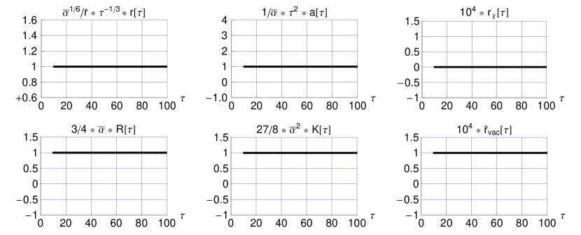
Figure 1: Numerical solution of the ODEs (30) with source term (32) and parameters $w_{M}=1/3$, $\mu=-3$, $\lambda=10^{-4}$, and $\gamma=0$ (quantum-dissipative effects inoperative). The initial boundary conditions are taken from the analytic de-Sitter-type solution (24) and (27), with $\overline{\alpha}\equiv\alpha_{\text{deS-spec-sol}}=132.629$ and $\overline{r}\equiv r_{\text{deS-spec-sol}}=0.800821$. Specifically, the boundary conditions at $\tau=\tau_{\text{bcs}}=10$ are: $\{a,r,\dot{r},r_{\chi}\}$ $=$ $\{1.32629119,0.764004165,0.02546680549,0\}$, where the $\dot{r}$ value has been obtained from the first Friedman equation (31). The top row shows the three basic variables: the two metric functions $r(\tau)$ and $a(\tau)$, and the dimensionless matter energy density $r_{\chi}$. The bottom row shows three derived quantities: the dimensionless Ricci curvature scalar $\mathcal{R}$, the dimensionless Kretschmann curvature scalar $\mathcal{K}$, and the dimensionless gravitating vacuum energy density $\widetilde{r}_{\text{vac}}$ from (30d). The vacuum energy density from the initial conditions is $\widetilde{r}_{\text{vac}}(\tau_{\text{bcs}})=1\times 10^{-4}$, which stays essentially constant.

We start from the special de-Sitter-type configuration as given in Sec. III.3.2. Numerical results, for $\mu=-3$ and $\lambda=10^{-4}$, are presented in Figs. 1 and 2 with two values of the vacuum-matter-energy-exchange coupling constant $\gamma$. The numerical solution of Fig. 1 with $\gamma=0$ essentially reproduces the special de-Sitter-type solution of Sec. III.3.2, whereas the numerical solution of Fig. 2 with $\gamma=2\times 10^{11}$ shows the rapid reduction of the vacuum energy density $\widetilde{r}_{\text{vac}}$ and the approach to the analytic Friedmann-type solution of Sec. III.3.1. The results in Figs. 1 and 2 resemble those in Figs. 9 and 10 of Ref. Klinkhamer2022-ext-unimod , but there are significant differences as regards the value of the chemical potential $\mu$, the initial condition on $r(\tau)$, and the value of the scaling factor $\overline{r}$.

We have two important remarks regarding the comparison of the vacuum energy density results obtained here and those obtained previously. First, we note that $(\mu-\lambda)<0$ does not allow for the nullification of the vacuum energy density for the case of the linear $\epsilon$ Ansatz (3), which was the Ansatz used in Ref. Klinkhamer2022-ext-unimod . Second, the $r_{\text{vac}}$ panels of Fig. 10 in Ref. Klinkhamer2022-ext-unimod and the $\widetilde{r}_{\text{vac}}$ panels of Fig. 2 here are identical within the numerical accuracy, because the resulting ODE (33) for $\widetilde{r}_{\text{vac}}(\tau)$ and the corresponding ODE for $r_{\text{vac}}(\tau)$ in Ref. Klinkhamer2022-ext-unimod have the same structure and the same boundary value $10^{-4}$ at $\tau=10$, the only difference being the “internal” structure of $\widetilde{r}_{\text{vac}}(\tau)$ and $r_{\text{vac}}(\tau)$.

To summarize, we have shown in Ref. Klinkhamer2022-ext-unimod and the present paper that, in principle, the cosmological constant $\Lambda$ can be cancelled by the field $\sqrt{-g}$ and appropriate quantum-dissipative effects (in principle, there can be other vacuum-matter energy-exchange mechanisms). For completeness, we have also given, in App. C of Ref. Klinkhamer2022-ext-unimod , numerical results on the readjustment after a phase transition.

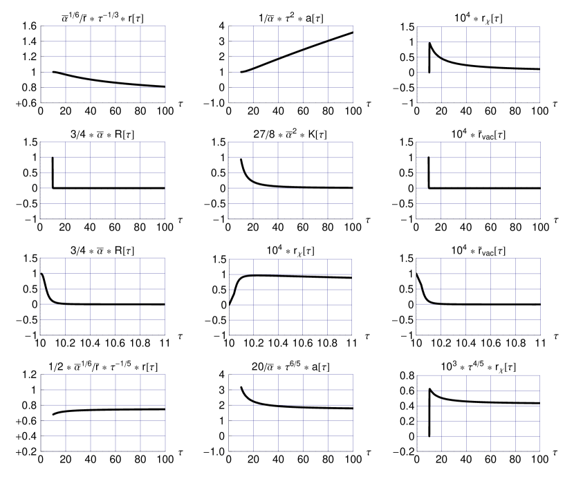
Figure 2: Numerical solution of the ODEs (30) with source term (32), where the boundary conditions at $\tau=\tau_{\text{bcs}}=10$ and the model parameters are the same as in Fig. 1, but now with $\gamma=2\times 10^{11}$ (quantum-dissipative effects operative). The vacuum energy density is initially $\widetilde{r}_{\text{vac}}(10)=1\times 10^{-4}$ and drops to $\widetilde{r}_{\text{vac}}(100)\sim 4\times 10^{-10}$. The third row shows the smooth behavior near the initial boundary conditions and the fourth row the asymptotic Friedmann-type behavior.

V Emergent gravity

V.1 Spacetime crystal: Elasticity tetrads

A possible explanation of the hypothesis presented in Sec. II.1 is that gravity is not a fundamental interaction but rather an emergent phenomenon. One explicit suggestion was outlined in Ref. Klinkhamer2022-ext-unimod and will be briefly reviewed here. Another explicit suggestion will be discussed in the next subsection.

In Sec. IV of Ref. Klinkhamer2022-ext-unimod , we have considered the following matter Lagrange density term for a real scalar field $\phi$:

$$\epsilon(\phi,\,n) = \widetilde{\epsilon}\,(\phi)\left(1+\zeta\,M^{-4}\,n\right)\,,$$ (34a)

with a positive dimensionless constant $$\zeta$$, the definition

$$n(x)\equiv E(x)=M^{4}\,\sqrt{-g(x)}\,,$$ (34b)

and now an explicit example of the function $$\widetilde{\epsilon}$$,

$$\widetilde{\epsilon}\,(\phi) = M^{4}\,+\frac{1}{2}\,M^{2}\,\phi^{2}\,,$$ (34c)

where $M$ is a single mass scale (possibly of the order of the Planck energy). The resulting gravitating vacuum energy density is Klinkhamer2022-ext-unimod

$$\rho_{\text{vac}}(\phi,n) = \widetilde{\epsilon}\,(\Phi)\left(1+2\,\zeta\,M^{-4}\,n\right)-\mu\,M^{4}\,,$$ (35)

where $\mu$ is the chemical potential corresponding to the conservation of the spacetime points of a hypothetical crystal.

The quantity $E$ in (34b) stands for the determinant of the elasticity tetrads of the spacetime crystal (see Sec. II of Ref. Klinkhamer2022-ext-unimod and especially Ref. NissinenVolovik2019 for further background on elasticity tetrads). With the assumption of gravity arising from these elasticity tetrads, $E$ is then identified with the square root of minus the metric determinant, $E\propto\sqrt{-g}$, where the minus sign holds for a Lorentzian signature of the emergent spacetime metric $g_{\alpha\beta}$.

Even though the elasticity tetrads can, in principle, produce a nonstandard term ${\textstyle\frac{1}{2}}\,M^{2}\,\phi^{2}\,\sqrt{-g}$ as in (34a), it is not clear how this would really come about. In this respect, an explicit suggestion based on a matrix model is perhaps more compelling, and such a suggestion will be discussed next.

V.2 IIB matrix model

V.2.1 Emerging spacetime

It has been submitted that the IIB matrix model IKKT-1997 ; Aoki-etal-review-1999 can give rise to some type of spacetime lattice and an emergent spacetime metric. The authors of Ref. Aoki-etal-review-1999 , in particular, have argued that “the space-time is dynamically determined from the eigenvalue distributions of the matrices” (quote from the Abstract) and that “the invariance under a permutation of the eigenvalues leads to the invariance of the low-energy effective action under general coordinate transformations” (quote from Sec. 4.2). Most likely, the basic idea is correct, but, strictly speaking, the matrices in Refs. IKKT-1997 ; Aoki-etal-review-1999 are mere integration variables and there is no small dimensionless parameter to motivate a saddle-point approximation. A possible solution of this puzzle has been provided by the recent suggestion that the so-called master field controls the emergence of a classical spacetime, indeed as eigenvalues but now the eigenvalues of the IIB-matrix-model master-field matrices.

This new conceptual idea was proposed in Ref. Klinkhamer2021-master , which also contains an explicit procedure on how to extract the classical spacetime from the IIB-matrix-model master-field matrices. Meanwhile, several follow-up research papers have appeared in Ref. Klinkhamer2021-IIBmm-regulBB ; Klinkhamer2021-IIBmm-master-field-sol-1 ; Klinkhamer2021-IIBmm-master-field-sol-2 ; Klinkhamer2021-IIBmm-master-field-sol-3 , together with two comprehensive reviews Klinkhamer2021-EpiphanyConf ; Klinkhamer2022-CorfuConf .

Here, we intend to show that this matrix-model approach can also provide a possible explanation of nonstandard terms in the matter Lagrange density involving the metric determinant. As a preparation for this discussion, we have collected in App. A.1 the main steps of how the information about the emergent spacetime points $\widehat{x}^{\,\alpha}_{k}$ is encoded in the master-field matrices. These discrete spacetime points $\widehat{x}^{\,\alpha}_{k}$ are labeled by $k\in\{1,\,\ldots,\,K\}$, with $K$ a divisor of $N$.

V.2.2 Discrete effective action

From appropriate perturbations of the master-field matrices $\widehat{A}^{\,\alpha}$ (restricting to $D=4$ “large” Euclidean dimensions), the following effective action can be obtained for a low-energy scalar degree of freedom $\phi$ propagating over the discrete spacetime points $\widehat{x}^{\,\alpha}_{k}$:

$$S_{\text{eff}}[\phi_{k},\,\eta_{k},\,\ldots] \supset \sum_{k=1}^{K}\;\sum_{l=1}^{K}\;\frac{1}{2}\,\widetilde{f}\big{(}\widehat{x}_{k}-\widehat{x}_{l}\big{)}\,\ell^{2}\,\big{(}\phi_{k}-\phi_{l}\big{)}^{2}+\sum_{k=1}^{K}\;\frac{1}{2}\,\widetilde{m}^{2}\,\ell^{2}\,\big{(}\phi_{k}\big{)}^{2}$$ (36)

$$+\sum_{k=1}^{K}\;\sum_{l=1}^{K}\;\widetilde{h}\big{(}\widehat{x}_{k}-\widehat{x}_{l}\big{)}\,\big{(}\phi_{k}\big{)}^{2}\,\big{(}\eta_{l}\big{)}^{2},$$

where $\widetilde{f}(x)$ and $\widetilde{h}(x)$ are steep dimensionless functions centered on $x=0$, the matrix perturbations $\phi_{k}$ and $\eta_{k}$ have the dimension of length, $\widetilde{m}$ is dimensionless, and $\ell$ is the model length scale Aoki-etal-review-1999 ; Klinkhamer2021-master (on the length scale issue, see also the last paragraph of Sec. 5 in Ref. Klinkhamer2022-CorfuConf ). The effective action can, of course, be expected to contain fields of all spins, but considering only scalar fields suffices for our purpose. Details on how the discrete scalar-field effective action (36) can be obtained are given in App. A.2.

We observe the permutation symmetry of the result (36):

$$\widehat{x}^{\,\alpha}_{k} \rightarrow \widehat{x}^{\,\alpha}_{\sigma(k)}\,,\quad\sigma\in S_{K}\,,$$ (37a)

with corresponding changes of the matrix perturbations, $\phi_{k}\rightarrow\phi_{\sigma(k)}$ and $\eta_{k}\rightarrow\eta_{\sigma(k)}$. The role of this permutation symmetry will be discussed further in Sec. V.2.4.

V.2.3 Standard action terms in the continuum

The first two terms in (36) were discussed in Refs. Aoki-etal-review-1999 ; Klinkhamer2021-master , but the last term is new. These first two terms give the following continuum effective action for a real scalar field $\phi(x)$ of mass dimension 1:

$$S_{\text{eff}}^{\text{kin+mass}}[\phi(x)]\sim\int d^{4}x\,\sqrt{|g(x)|}\;\left[\frac{1}{2}\;g^{\alpha\beta}(x)\;\partial_{\alpha}\phi(x)\,\partial_{\beta}\phi(x)\,+\frac{1}{2}\,m^{2}\;\phi^{2}\right]\,,$$ (38)

in terms of an emergent inverse metric $g^{\alpha\beta}$ and a classical dilaton field $\Phi$ (here, this dilaton field has been assumed constant and has been normalized away). Specifically, we have for these emerging fields

$$g^{\alpha\beta}(x) \sim \int_{\mathbb{R}^{4}}d^{4}y\;\rho(y)\;\ell^{-2}\,(x-y)^{\,\alpha}\,(x-y)^{\beta}\;r(x,\,y)\;f(x-y)\,,$$ (39a)

$$\sqrt{|g(x)|} \propto \rho(x)\,,$$ (39b)

with $g\equiv\det g_{\alpha\beta}$. The square root $\sqrt{|g(x)|}$ can also be written as $\sqrt{\pm g(x)}$, where the $\pm$ signs refer to the Euclidean or Lorentzian signatures of the emerging spacetime metric; see below for further comments. The quantities $\rho(x)$ and $r(x,\,y)$ entering the expressions (39) result from the distributions and correlations of the spacetime points $\widehat{x}^{\,\alpha}_{k}$ obtained from the master field; their definitions are given in App. A.1. The quantity $f(x)$ entering the expression (39a) traces back to the first term in (36), which results from perturbations of the master-field matrices; see App. A.2.

Equations (39a) and (39b) have essentially been given as Eqs. (4.17) and (4.18) in Ref. Aoki-etal-review-1999 , but here we have made clear precisely which matrices are considered for the eigenvalues, namely the master-field matrices $\widehat{A}^{\,\alpha}$ (the heuristics of the spacetime extraction from the master-field matrices is explained in Sec. 4.4 of Ref. Klinkhamer2021-EpiphanyConf ). For completeness, we mention that there have also been other approaches on getting an effective metric field from the IIB matrix model (see, e.g., Refs. Sakai2019 ; Steinacker2022 ; Brahma-etal2022 and references therein).

At this moment, we have three technical remarks, which can be skipped in a first reading. The first technical remark is that the signature of the emerging spacetime metric depends on the structure of the correlation functions of the spacetime points. Toy-model calculations have been presented in App. D of Ref. Klinkhamer2021-EpiphanyConf , which show that certain deformation parameters in the correlation functions allow for a continuous change from a Euclidean to a Lorentzian signature (passing through a degenerate metric with a vanishing eigenvalue).

The second technical remark is that, assuming the matrix size $N=K\,n$ to be large enough and the block size $n$ to be of the order of the band width $\Delta N$ (see App. A.1 for details), we need not average the $\rho$ functions appearing on the right-hand sides of (39). This averaging would be over different block sizes ($n$) and over different block positions along the diagonals of the master-field matrices . But these explicit averages would not be necessary if we have a genuine master field at an effectively infinite $N$ (for a general discussion of the role of master fields, see, in particular, Ref. Carlson-etal-1983 ).

The third technical remark is that the fermion dynamics plays an important role for the bosonic master-field matrices $\widehat{A}^{\,\alpha}$, as they are the solution of the so-called master-field equation which has a Pfaffian term due to the fermions. The master-field equation and its solutions have been studied in three recent papers Klinkhamer2021-IIBmm-master-field-sol-1 ; Klinkhamer2021-IIBmm-master-field-sol-2 ; Klinkhamer2021-IIBmm-master-field-sol-3 and have been reviewed in Ref. Klinkhamer2022-CorfuConf . (Recall that the fermion dynamics also played an important role in the original discussion of Ref. Aoki-etal-review-1999 by providing the so-called Boltzmann weights in the graphs considered.)

V.2.4 Nonstandard action term in the continuum

Now, turn to the third term in (36), which is new and has been “derived” in App. A.2. For a steep function $\widetilde{h}\big{(}\widehat{x}_{k}-\widehat{x}_{l}\big{)}$, having $\widetilde{h}\sim 0$ for $\widehat{x}_{k}\neq\widehat{x}_{l}$, and constant perturbations $\eta_{k}$,

$$\eta_{k}=\overline{\eta}\,,$$ (40)

we get the following nonstandard term in the continuum effective action:

$$S_{\text{eff}}^{\text{(nonstandard)}}[\phi(x)]\sim\int d^{4}x\,\sqrt{|g(x)|}\;\Big{[}\;\phi^{2}(x)\;\sqrt{|g(x)|}\;\eta^{2}\Big{]}\,,$$ (41)

where $\eta$ is a constant real scalar field of mass dimension 1 tracing back to the rescaled constant matrix perturbation $\overline{\eta}/\ell^{2}$.

Incidentally, by taking also $\phi_{k}$ constant, $\phi_{k}=\overline{\eta}$, we get the action term (41) with the integrand $\big{[}\eta^{2}\,\sqrt{|g(x)|}\>\eta^{2}\big{]}$, corresponding to the linear $\zeta$ term appearing in our previous $\epsilon$ Ansatz (3). It appears impossible to get, in this way, negative powers of $n\propto\sqrt{|g|}$, as used in the extended $\epsilon$ Ansatz (9). Still, there may appear divergent powers series in $n$, which, for example, sum to $\epsilon$ functions of the form $\lambda+n^{2}/(n-1)$ or $\lambda+n\,\cos(2\pi\,n)$, allowing for the cancellation of any value of $(\lambda-\mu)$ in the corresponding $r_{\text{vac}}$ functions.

The action term (41) is, of course, only invariant under restricted coordinate transformations with unit Jacobian (1). Let us, therefore, briefly discuss the issue of diffeomorphisms.

The authors of Ref. Aoki-etal-review-1999 have given a plausibility argument that the permutation symmetry over the discrete spacetime points implies the diffeomorphism invariance of the continuum theory. But the delicate issue of how simultaneously the locality appears in the continuum theory is far from resolved. We suspect that the nonstandard term (41), which is local but not fully diffeomorphism invariant, appears due to some type of interference between the emergence of locality and the emergence of diffeomorphism invariance (we are reminded of the appearance of anomalies in chiral gauge theories). Anyway, let us have a closer look at how precisely the surprising term (41) arises in our calculation.

The actual way how the third term of (36) appears is from both the “internal space” of each spacetime point individually and the larger group space of the matrices acting between different spacetime points. Specifically, referring to (48) in App. A.2 and fixing $k=1$ for convenience, the origin of the $\phi_{1}^{2}\,\eta_{1}^{2}$ term lies in the $\zeta_{1}$ entries inside the first $4\times 4$ block on the diagonal and the origin of the $\left(\phi_{1}^{2}\,\eta_{2}^{2}+\phi_{2}^{2}\,\eta_{1}^{2}\right)$ and $\left(\phi_{1}^{2}\,\eta_{3}^{2}+\phi_{3}^{2}\,\eta_{1}^{2}\right)$ terms in the $\xi_{12}$ and $\xi_{13}$ entries “coupling” the different $4\times 4$ spacetime blocks.

The crucial observation now is that the way how, for $k\neq l$, the action terms $\left(\phi_{k}^{2}\,\eta_{l}^{2}+\phi_{l}^{2}\,\eta_{k}^{2}\right)$ arise is essentially the same as for the action terms $\left(\phi_{k}-\phi_{l}\right)^{2}$; see the last two paragraphs in App. A.2. Both of these terms involve a double sum, each of which gives a density function $\rho$ for the continuum expression, as shown by (46). For the kinetic type terms, one density function $\rho$ gets absorbed into the definition of the emerging inverse metric, as the expression (39a) makes clear. But for the mixed $\phi_{k}^{2}\,\eta_{l}^{2}$ terms, there remains one extra density function $\rho$ in what will become the continuum Lagrange density and precisely that $\rho$ gives the $\sqrt{|g(x)|}$ factor inside the square brackets on the right-hand side of (41).

In short, if we can get the double-sum kinetic-type terms with $\left(\phi_{k}-\phi_{l}\right)^{2}$ in the discrete effective action (36), then it is also possible to get the double-sum mixed terms with $\phi_{k}^{2}\,\eta_{l}^{2}$. The first double sum gives the kinetic term in the continuum action (38), while the second double sum gives the nonstandard term (41).

In closing, we have a peripheral remark. We observe, namely, that (39a) has a direct dependence on the matter function $f$, whereas (39b) does not. Starting from the inverse metric components (39a), we can, of course, calculate the determinant, but then all influence of the matter function $f$ must somehow “average out.” In any case, taking the expressions (39a) and (39b) at face value, it is clear that the metric determinant appears to play a special role and it is perhaps not surprising to have additional $\sqrt{|g(x)|}$ factors turn up in the continuum matter Lagrange density.

VI Discussion

In a previous paper Klinkhamer2022-ext-unimod , we have explored a cosmological model with a dynamic metric-determinant field $g(x)\equiv\det g_{\alpha\beta}(x)$, thereby reducing the allowed coordinate transformations to those with a unit Jacobian. Some further new results were presented in Secs. III and IV here.

The origin of the nonstandard terms in the matter Lagrange density with one or more additional factors of $\sqrt{|g(x)|}$, for example the term from (41), still needs to be established firmly. Here, we have presented an explicit calculation based on the so-called IIB matrix model, which provides a nonperturbative formulation of superstring theory. Our basic argument is given in Sec. V.2.4, with technical details relegated to App. A.2. Considering the effective action of a real scalar field $\phi(x)$, it appears equally easy to get the standard kinetic term ${\textstyle\frac{1}{2}}\;g^{\alpha\beta}\;\partial_{\alpha}\phi\,\partial_{\beta}\phi$ in the Lagrange density as nonstandard terms $\phi^{2}\,\sqrt{|g|}\,\eta^{2}$ or $\eta^{2}\,\sqrt{|g|}\,\eta^{2}$, for a constant real scalar field $\eta$. These nonstandard terms are local but only invariant under restricted coordinate transformations. The simultaneous appearance of locality and (restricted) diffeomorphism invariance needs, of course, to be studied further. The same holds for other approaches to metric-field extraction from the IIB matrix model Sakai2019 ; Steinacker2022 ; Brahma-etal2022 .

Anyway, the matrix-model calculation of the present paper alerts us to the possibility that there may be rather unusual interactions in the effective low-energy theory. In fact, the nonstandard action term in (41) corresponds to a type of variable mass square for the scalar field, where the effective mass square involves the metric determinant $g(x)$. As the metric determinant $g(x)$ depends on the environment through the field equations, there is an obvious resemblance with the chameleon scenario KhouryWeltman2003-PRL ; KhouryWeltman2003-PRD . Considering a Lagrange-density term ${\textstyle\frac{1}{2}}\,g^{2}\,m^{2}\,\phi^{2}$, for example, we can perform a simple nonrelativistic analysis using Poisson’s equation and find some possibly interesting behavior, but we postpone further discussion to a future publication.

Appendix A IIB-matrix-model calculation

A.1 Emerging spacetime points from master-field matrices

The bosonic action of the Euclidean IIB matrix model IKKT-1997 ; Aoki-etal-review-1999 reads

$$S_{\text{bos}}=-\frac{1}{2}\,\text{Tr}\,\Big{(}\big{[}A^{\alpha},\,A^{\beta}\big{]}\,\big{[}A^{\gamma},\,A^{\delta}\big{]}\,\delta_{\gamma\alpha}\,\delta_{\delta\beta}\Big{)}\,,$$ (42)

where the bosonic matrices $A^{\alpha}$, with a directional index $\alpha$ running over $\{1,\,\ldots\,,D\}$, are $N\times N$ traceless Hermitian matrices and the commutators are defined by $[B,\,C]\equiv$ $B\cdot C-C\cdot B$ for square matrices $B$ and $C$ of equal dimension. The action involves the Kronecker delta $\delta_{\gamma\alpha}$, which corresponds to a Euclidean “metric.” With matrices $A^{\alpha}$ of the dimension of length (these matrices will ultimately give the spacetime points $x^{\alpha}$), the dimension of the action (42) is $(\text{length})^{4}$ and the matrix integrals for the expectation values have a weight factor $\exp[-S_{\text{bos}}/\ell^{4}]$ for a model length scale $\ell$. The genuine IIB matrix model has dimensionality $D=10$. In this subsection, we keep $D$ general but, elsewhere, we set $D=4$ when four “large” dimensions are considered.

Assume that the master-field matrices $\widehat{A}^{\,\alpha}$ of the Euclidean IIB matrix model are known and that they are more or less band-diagonal (with a width $1<\Delta N\ll N$), as suggested by exploratory numerical results in Refs. KimNishimuraTsuchiya2012 ; NishimuraTsuchiya2019 ; Anagnostopoulos-etal-2020 and references therein. Now, let $K$ be a divisor of $N$, so that

$$N=K\,n\,,$$ (43)

where both $K$ and $n$ are positive integers. In the master-field matrices $\widehat{A}^{\,\alpha}$ with a band-diagonal structure, consider the $K$ blocks of size $n\times n$ centered on the diagonals (with $n\gtrsim\Delta N$ and $n\ll N$) and calculate the averages of the eigenvalues of these blocks. The obtained averages correspond to the emergent spacetime points and are denoted

$$\widehat{x}^{\,\alpha}_{k}\,,$$ (44)

where $\alpha$ runs over $\{1,\,\ldots,\,D\}$ and $k$ over $\{1,\,\ldots,\,K\}$, with $K$ as given by (43). Further comments on the extraction procedure appear in App. A of Ref. Klinkhamer2021-EpiphanyConf .

The quantities $\rho(x)$, $r(x,\,y)$, and $f(x)$ entering expressions (39) in the main text result from the distributions and correlations of the emerging spacetime points (44) and, as regards $f(x)$, from perturbations of the master-field matrices.

Specifically, the density function $\rho(x)$ and the density correlation function $r(x,\,y)$ are defined by

$$\rho(x) \equiv \sum_{k=1}^{K}\;\delta^{(D)}\big{(}x-\widehat{x}_{k}\big{)}\,,$$ (45a)

$$\langle\,\rho(x)\,\rho(y)\,\rangle \equiv \langle\,\rho(x)\,\rangle\;\langle\,\rho(y)\,\rangle\;r(x,\,y)\,,$$ (45b)

where $x^{\alpha}$ and $y^{\alpha}$ are $D$-dimensional continuous (interpolating) coordinates. The averages $\langle\,\ldots\,\rangle$ in (45b) stand for averaging over different block sizes ($n$) and over different block positions along the diagonals of the master-field matrices $\big{(}\widehat{A}^{\,\alpha}\big{)}_{kl}$ [note that the block at the beginning of the diagonal has dimension $n^{\prime}\leq n$ and the block at the end has dimension $n^{\prime\prime}\leq n$, but there are many more intermediate $n\times n$ blocks if $K\gg 1$]. In this way, the double sum in (36) is transformed into a double integral over the continuum spacetime,

$$\sum_{k,\,l}\;s\big{(}\widehat{x}_{k}-\widehat{x}_{l}\big{)}\,\ldots\;\rightarrow\int d^{D}x\,\langle\,\rho(x)\,\rangle\;\int d^{D}y\,\langle\,\rho(y)\,\rangle\;r(x-y)\,s(x-y)\ldots\;,$$ (46)

for an arbitrary function $s(x)$.

Finally, the quantity $f(x)$ entering expression (39a) in the main text is a localized real function coming from the “hopping” term with $\widetilde{f}\big{(}\widehat{x}_{k}-\widehat{x}_{l}\big{)}$ in the discrete scalar effective action (36).

A.2 Perturbations of master-field matrices

We present here a simple construction to obtain the third term of the discrete effective action (36). Essentially, this is a variation of the construction method developed in App. A of Ref. Klinkhamer2021-master . We focus on the four “large” dimensions (whose appearance may be suggested by exploratory numerical results in Ref. KimNishimuraTsuchiya2012 ; NishimuraTsuchiya2019 ; Anagnostopoulos-etal-2020 and references therein) and set $D=4$ in our expressions.

Take, now, the particular matrix sizes

$$N=4+4\,j+4\,,\quad j=1,\,2,\,3,\ldots\,.$$ (47)

Then, the first and last $4\times 4$ blocks on the diagonal will give $\phi_{k}^{2}\,\eta_{k}^{2}$ terms in (36) for the smallest and largest values of $k$ and the band diagonal in between (with suitable $4\times 4$ and $2\times 2$ blocks) will give both $\phi_{k}^{2}\,\eta_{k}^{2}$ terms and $[\phi_{k}^{2}\,\eta_{k\pm 1}^{2}+\phi_{k\pm 1}^{2}\,\eta_{k}^{2}]$ terms for intermediate values of $k$. Other far-off entries will give the $[\phi_{k}^{2}\,\eta_{l}^{2}+\phi_{l}^{2}\,\eta_{k}^{2}]$ terms for $|k-l|\geq 2$. All this will become clearer for the $j=1$ case to be discussed next.

Indeed, let us focus on the case $N=12$, where the master-field-type matrices have three $4\times 4$ blocks on the diagonal, labeled by $k\in\{1,\,2,\,3\}$. The basic structure of the perturbed matrices, with five $2\times 2$ blocks on the diagonal and two far-off entries (with $\xi_{13}$ and $\xi_{13}^{*}$), is then as follows (with lines added to mark the $4\times 4$ blocks):

$$A^{4}_{\text{tmp}} \!\!=\! \!\left(\begin{array}[]{cccc|cccc|cccc}\widehat{x}^{\,4}_{1}&0&0&0&0&0&0&0&0&0&0&0\\ 0&\widehat{x}^{\,4}_{1}&h^{4}\,\zeta_{1}&0&0&0&0&0&0&0&0&0\\ 0&h^{4}\,\zeta_{1}&\widehat{x}^{\,4}_{1}+\zeta_{1}&0&0&0&0&0&0&0&0\\ 0&0&0&\widehat{x}^{\,4}_{1}&\xi_{12}&0&0&0&\xi_{13}&0&0&0\\ \hline\cr 0&0&0&\xi_{12}^{*}&\widehat{x}^{\,4}_{2}&0&0&0&0&0&0&0\\ 0&0&0&0&0&\widehat{x}^{\,4}_{2}&i^{4}\,\zeta_{2}&0&0&0&0&0\\ 0&0&0&0&0&i^{4}\,\zeta_{2}&\widehat{x}^{\,4}_{2}+\zeta_{2}&0&0&0&0&0\\ 0&0&0&0&0&0&0&\widehat{x}^{\,4}_{2}&\xi_{23}&0&0&0\\ \hline\cr 0&0&0&\xi_{13}^{*}&0&0&0&\xi_{23}^{*}&\widehat{x}^{\,4}_{3}&0&0&0\\ 0&0&0&0&0&0&0&0&0&\widehat{x}^{\,4}_{3}&j^{4}\,\zeta_{3}&0\\ 0&0&0&0&0&0&0&0&0&j^{4}\,\zeta_{3}&\widehat{x}^{\,4}_{3}+\zeta_{3}&0\\ 0&0&0&0&0&0&0&0&0&0&0&\widehat{x}^{\,4}_{3}\\ \end{array}\right)\!-\Sigma^{4}\makebox[2.58334pt][l]{$1$}{\rm l}_{12}\,.$$ (48m)

where $$\makebox[2.58334pt][l]{$1$}{\rm l}_{12} 12\times 12 \Sigma^{4} h^{4} i^{4} j^{4} \zeta_{1} \zeta_{2} \zeta_{3} \xi_{kl} \widehat{x}^{\,4}_{k}$$ is the identity matrix and makes for tracelessness. The coefficients , , , , , and are real, whereas the coefficients are complex. The three other matrices are obtained by straightforward substitutions of the :

$$A^{1}_{\text{tmp}}=$$

$$A^{4}_{\text{tmp}}\;\text{with}\;\{\widehat{x}^{\,4}_{1}\to\widehat{x}^{\,1}_{1},\,\widehat{x}^{\,4}_{2}\to\widehat{x}^{\,1}_{2},\,\widehat{x}^{\,4}_{3}\to\widehat{x}^{\,1}_{3},\,h^{4}\to 0,\,i^{4}\to 0,\,j^{4}\to 0,\,\Sigma^{4}\to\Sigma^{1}\}\,,$$ (48n)

$$A^{2}_{\text{tmp}}=$$

$$A^{4}_{\text{tmp}}\;\text{with}\;\{\widehat{x}^{\,4}_{1}\to\widehat{x}^{\,2}_{1},\,\widehat{x}^{\,4}_{2}\to\widehat{x}^{\,2}_{2},\,\widehat{x}^{\,4}_{3}\to\widehat{x}^{\,2}_{3},\,h^{4}\to 0,\,i^{4}\to 0,\,j^{4}\to 0,\,\Sigma^{4}\to\Sigma^{2}\}\,,$$ (48o)

$$A^{3}_{\text{tmp}}=$$

$$A^{4}_{\text{tmp}}\;\text{with}\;\{\widehat{x}^{\,4}_{1}\to\widehat{x}^{\,3}_{1},\,\widehat{x}^{\,4}_{2}\to\widehat{x}^{\,3}_{2},\,\widehat{x}^{\,4}_{3}\to\widehat{x}^{\,3}_{3},\,h^{4}\to 0,\,i^{4}\to 0,\,j^{4}\to 0,\,\Sigma^{4}\to\Sigma^{3}\}\,,$$ (48p)

where, for simplicity, the $h^{\alpha}$, $i^{\alpha}$, and $j^{\alpha}$ terms have been set to zero for $\alpha=1,\,2,\,3$.

Next, insert the real perturbations $\phi_{k}$ and $\eta_{k}$ (each with the dimension of length) into the above matrices:

$$\{A^{4},\,A^{1},\,A^{2},\,A^{3}\}=$$

$$\{A^{4}_{\text{tmp}},\,A^{1}_{\text{tmp}},\,A^{2}_{\text{tmp}},\,A^{3}_{\text{tmp}}\}\;\text{with}\;$$

$$\Big{\{}{\zeta_{1}}\rightarrow\left({\eta_{1}}^{2}\,{\phi_{1}}^{2}\right)^{1/4},\;\;{\zeta_{2}}\rightarrow\left({\eta_{2}}^{2}\,{\phi_{2}}^{2}\right)^{1/4},\;\;{\zeta_{3}}\rightarrow\left({\eta_{3}}^{2}\,{\phi_{3}}^{2}\right)^{1/4},$$

$$\xi_{12}\rightarrow\widetilde{g}_{12}\,\ell^{-1}\,\left(\eta_{2}\,\phi_{1}+i\,\eta_{1}\,\phi_{2}\right),\;\;\xi_{12}^{*}\rightarrow\widetilde{g}_{12}\,\ell^{-1}\,\left(\eta_{2}\,\phi_{1}-i\,\eta_{1}\,\phi_{2}\right),$$

$$\xi_{13}\rightarrow\widetilde{g}_{13}\,\ell^{-1}\,\left(\eta_{3}\,\phi_{1}+i\,\eta_{1}\,\phi_{3}\right),\;\;\xi_{13}^{*}\rightarrow\widetilde{g}_{13}\,\ell^{-1}\,\left(\eta_{3}\,\phi_{1}-i\,\eta_{1}\,\phi_{3}\right),$$

$$\xi_{23}\rightarrow\widetilde{g}_{23}\,\ell^{-1}\,\left(\eta_{3}\,\phi_{2}+i\,\eta_{2}\,\phi_{3}\right),\;\;\xi_{23}^{*}\rightarrow\widetilde{g}_{23}\,\ell^{-1}\,\left(\eta_{3}\,\phi_{2}-i\,\eta_{2}\,\phi_{3}\right)\Big{\}}\,,$$ (49)

with real dimensionless coefficients $\widetilde{g}_{12},\,\widetilde{g}_{13},\,\widetilde{g}_{23}$ that depend on the differences of the spacetime points, $\widetilde{g}_{12}=\widetilde{g}_{12}(\widehat{x}^{\,\alpha}_{1}-\widehat{x}^{\,\alpha}_{2})$ and similarly for $\widetilde{g}_{13}$ and $\widetilde{g}_{23}$. Observe that the same coefficients $\zeta_{k}$ and $\xi_{kl}$ enter all matrices $A^{\alpha}_{\text{tmp}}$ identically and precisely these coefficients give the perturbations by the substitutions (A.2); this crucial point has been emphasized in the second paragraph of App. A in Ref. Klinkhamer2021-master .

Evaluating the bosonic action (42) for the perturbation matrices (A.2) gives

$$S_{\text{bos}}^{\text{(pert)}} = \frac{1}{2}\,\ell^{-2}\,D_{12}\,{\widetilde{g}_{12}}^{\,2}\,\left({\eta_{1}}^{2}\,{\phi_{2}}^{2}+{\eta_{2}}^{2}\,{\phi_{1}}^{2}\right)+\frac{1}{2}\,\ell^{-2}\,D_{13}\,{\widetilde{g}_{13}}^{\,2}\,\left({\eta_{1}}^{2}\,{\phi_{3}}^{2}+{\eta_{3}}^{2}\,{\phi_{1}}^{2}\right)+$$ (50a)

$$\frac{1}{2}\,\ell^{-2}\,D_{23}\,{\widetilde{g}_{23}}^{\,2}\,\left({\eta_{2}}^{2}\,{\phi_{3}}^{2}+{\eta_{3}}^{2}\,{\phi_{2}}^{2}\right)+$$

$$\frac{1}{2}\,\left[3\,\left(h^{4}\right)^{2}\,{\eta_{1}}^{2}\,{\phi_{1}}^{2}+3\,\left(i^{4}\right)^{2}\,{\eta_{2}}^{2}\,{\phi_{2}}^{2}+3\,\left(j^{4}\right)^{2}\,{\eta_{3}}^{2}\,{\phi_{3}}^{2}\right]\,,$$

with

$$D_{12} = 3\,\left({\Delta\widehat{x}^{\,1}_{21}}\right)^{2}+3\,\left({\Delta\widehat{x}^{\,2}_{21}}\right)^{2}+3\,\left({\Delta\widehat{x}^{\,3}_{21}}\right)^{2}-2\,\Delta\widehat{x}^{\,3}_{21}\,\Delta\widehat{x}^{\,4}_{21}+3\,\left({\Delta\widehat{x}^{\,4}_{21}}\right)^{2}-$$

$$2\,\Delta\widehat{x}^{\,2}_{21}\,\left(\Delta\widehat{x}^{\,3}_{21}+\Delta\widehat{x}^{\,4}_{21}\right)-2\,\Delta\widehat{x}^{\,1}_{21}\,\left(\Delta\widehat{x}^{\,2}_{21}+\Delta\widehat{x}^{\,3}_{21}+\Delta\widehat{x}^{\,4}_{21}\right)\,,$$ (50b)

$$D_{13} = 3\,\left({\Delta\widehat{x}^{\,1}_{21}}\right)^{2}+3\,\left({\Delta\widehat{x}^{\,1}_{32}}\right)^{2}+3\,\left({\Delta\widehat{x}^{\,2}_{21}}\right)^{2}-6\,\Delta\widehat{x}^{\,2}_{21}\,\Delta\widehat{x}^{\,2}_{32}+3\,\left({\Delta\widehat{x}^{\,2}_{32}}\right)^{2}-$$ (50c)

$$2\,\Delta\widehat{x}^{\,2}_{21}\,\Delta\widehat{x}^{\,3}_{21}+2\,\Delta\widehat{x}^{\,2}_{32}\,\Delta\widehat{x}^{\,3}_{21}+3\,\left({\Delta\widehat{x}^{\,3}_{21}}\right)^{2}+2\,\Delta\widehat{x}^{\,2}_{21}\,\Delta\widehat{x}^{\,3}_{32}-$$

$$2\,\Delta\widehat{x}^{\,2}_{32}\,\Delta\widehat{x}^{\,3}_{32}-6\,\Delta\widehat{x}^{\,3}_{21}\,\Delta\widehat{x}^{\,3}_{32}+3\,\left({\Delta\widehat{x}^{\,3}_{32}}\right)^{2}-2\,\Delta\widehat{x}^{\,2}_{21}\,\Delta\widehat{x}^{\,4}_{21}+$$

$$2\,\Delta\widehat{x}^{\,2}_{32}\,\Delta\widehat{x}^{\,4}_{21}-2\,\Delta\widehat{x}^{\,3}_{21}\,\Delta\widehat{x}^{\,4}_{21}+2\,\Delta\widehat{x}^{\,3}_{32}\,\Delta\widehat{x}^{\,4}_{21}+3\,\left({\Delta\widehat{x}^{\,4}_{21}}\right)^{2}+$$

$$2\,\Delta\widehat{x}^{\,1}_{32}\,\left(\Delta\widehat{x}^{\,2}_{21}-\Delta\widehat{x}^{\,2}_{32}+\Delta\widehat{x}^{\,3}_{21}-\Delta\widehat{x}^{\,3}_{32}+\Delta\widehat{x}^{\,4}_{21}-\Delta\widehat{x}^{\,4}_{32}\right)-$$

$$2\,\Delta\widehat{x}^{\,1}_{21}\,\left(3\,\Delta\widehat{x}^{\,1}_{32}+\Delta\widehat{x}^{\,2}_{21}-\Delta\widehat{x}^{\,2}_{32}+\Delta\widehat{x}^{\,3}_{21}-\Delta\widehat{x}^{\,3}_{32}+\Delta\widehat{x}^{\,4}_{21}-\Delta\widehat{x}^{\,4}_{32}\right)+$$

$$2\,\Delta\widehat{x}^{\,2}_{21}\,\Delta\widehat{x}^{\,4}_{32}-2\,\Delta\widehat{x}^{\,2}_{32}\,\Delta\widehat{x}^{\,4}_{32}+2\,\Delta\widehat{x}^{\,3}_{21}\,\Delta\widehat{x}^{\,4}_{32}-$$

$$2\,\Delta\widehat{x}^{\,3}_{32}\,\Delta\widehat{x}^{\,4}_{32}-6\,\Delta\widehat{x}^{\,4}_{21}\,\Delta\widehat{x}^{\,4}_{32}+3\,\left({\Delta\widehat{x}^{\,4}_{32}}\right)^{2}\,,$$

$$D_{23} = 3\,\left({\Delta\widehat{x}^{\,1}_{32}}\right)^{2}+3\,\left({\Delta\widehat{x}^{\,2}_{32}}\right)^{2}+3\,\left({\Delta\widehat{x}^{\,3}_{32}}\right)^{2}-2\,\Delta\widehat{x}^{\,3}_{32}\,\Delta\widehat{x}^{\,4}_{32}+3\,\left({\Delta\widehat{x}^{\,4}_{32}}\right)^{2}-$$ (50d)

$$2\,\Delta\widehat{x}^{\,2}_{32}\,\left(\Delta\widehat{x}^{\,3}_{32}+\Delta\widehat{x}^{\,4}_{32}\right)-2\,\Delta\widehat{x}^{\,1}_{32}\,\left(\Delta\widehat{x}^{\,2}_{32}+\Delta\widehat{x}^{\,3}_{32}+\Delta\widehat{x}^{\,4}_{32}\right)\,,$$

$$\Delta\widehat{x}^{\,\alpha}_{21} \equiv \widehat{x}^{\,\alpha}_{2}-\widehat{x}^{\,\alpha}_{1}\,,\quad\Delta\widehat{x}^{\,\alpha}_{32}\equiv\widehat{x}^{\,\alpha}_{3}-\widehat{x}^{\,\alpha}_{2}\,.$$ (50e)

The obtained discrete action (50a) has the dimension of $(\text{length})^{4}$ and its structure corresponds to the third term on the right-hand side of (36).

We can obtain the first two terms on the right-hand side of (36) by enlarging, for the master-field-type matrices, the $4\times 4$ blocks on the diagonal to, for example, $6\times 6$ blocks (corresponding to $N=6+6\,j+6$ with $j\in\mathbb{N}_{+}$). We have explicitly constructed the $N=18$ matrices by inserting appropriate $2\times 2$ entries centered on the diagonal with the $\kappa_{12}\equiv\widetilde{k}_{12}\,(\phi_{1}-\phi_{2})$ structure as given in App. A of Ref. Klinkhamer2021-master , by changing the $\zeta_{1}$ replacement to $\left({\eta_{1}}^{2}\,{\phi_{1}}^{2}+\ell^{2}\,{\phi_{1}}^{2}\right)^{1/4}$, and by adding further appropriate far-off terms $\kappa_{13}\equiv\widetilde{k}_{13}\,(\phi_{1}-\phi_{3})$ and $\kappa_{13}^{*}=\kappa_{13}$.

For the hopping terms $(\phi_{k}-\phi_{l})^{2}$ with $k\neq l$, the idea is that, by carefully choosing the rows and columns, these additional $2\times 2$ entries do not “interfere” with those already present in (48), which were designed to give the third term on the right-hand side of (36). The following $4\times 4$ part of the $18\times 18$ matrix $A^{\alpha}$ makes this point clear:

$$A^{\alpha}=\left(\begin{array}[]{cccccc}\ddots&\vdots&\vdots&\vdots&\vdots&\udots\\ \ldots&\widehat{x}^{\,\alpha}_{1}&0&0&\widetilde{k}_{12}\,(\phi_{1}-\phi_{2})&\ldots\\ \ldots&0&\widehat{x}^{\,\alpha}_{1}&\widetilde{g}_{12}\,\left(\phi_{1}\,\eta_{2}+i\,\phi_{2}\,\eta_{1}\right)&0&\ldots\\ \ldots&0&\widetilde{g}_{12}\,\left(\phi_{1}\,\eta_{2}-i\,\phi_{2}\,\eta_{1}\right)&\widehat{x}^{\,\alpha}_{2}&0&\ldots\\ \ldots&\widetilde{k}_{12}\,(\phi_{1}-\phi_{2})&0&0&\widehat{x}^{\,\alpha}_{2}&\ldots\\ \udots&\vdots&\vdots&\vdots&\vdots&\ddots\\ \end{array}\right),$$ (51)

for which the commutators from (42) give the action term with $\left(\phi_{1}^{2}\,\eta_{2}^{2}+\phi_{2}^{2}\,\eta_{1}^{2}\right)$ from the inner $2\times 2$ block and the action term with $(\phi_{1}-\phi_{2})^{2}$ from the outer $2\times 2$ “block.” Both of these $2\times 2$ entries in (51), the inner one and the outer one, have basically the same structure, with $\widehat{x}^{\,\alpha}_{1}$ and $\widehat{x}^{\,\alpha}_{2}$ on the diagonal and Hermitian conjugates on the counter-diagonal.