Optimal Control in Stochastic Thermodynamics

Abstract

We review recent progress in optimal control in stochastic thermodynamics. Theoretical advances provide in-depth insight into minimum-dissipation control with either full or limited (parametric) control, and spanning the limits from slow to fast driving and from weak to strong driving. Known exact solutions give a window into the properties of minimum-dissipation control, which are reproduced by approximate methods in the relevant limits. Connections between optimal-transport theory and minimum-dissipation protocols under full control give deep insight into the properties of optimal control and place bounds on the dissipation of thermodynamic processes. Since minimum-dissipation protocols are relatively well understood and advanced approximation methods and numerical techniques for estimating minimum-dissipation protocols have been developed, now is an opportune time for application to chemical and biological systems.

I Introduction

In this article we review recent progress in optimal control of stochastic thermodynamic systems. We focus on classical isothermal stochastic thermodynamics describing control by linear-response, thermodynamic geometry, and optimal-transport theory.

Historically, modern thermodynamic control began with the study of finite-time thermodynamics of macroscopic systems, Andresen et al. (1977); Salamon et al. (1977); Andresen (2011) the natural extension beyond quasistatic (infinitely slow) processes. Fundamentally, any finite-time thermodynamic control will induce some degree of irreversibility, manifesting as energy dissipated into the environment. A goal of finite-time thermodynamics is to quantify and minimize this dissipation through the use of designed control strategies. For example, Ref. Band et al., 1982 studied the optimal cycle for finite-time operation of a heat engine and found that instantaneous jumps in control parameters are necessary to minimize dissipation.

In parallel, a thermodynamic-geometry framework was developed to provide a novel means to describe thermodynamic processes on a smooth (generally Riemannian) manifold.Weinhold (1975); Ruppeiner (1979); Crooks (2007) Ref. Salamon and Berry, 1983 showed the connections between thermodynamic geometry and minimum-dissipation protocols, opening the door for the development of a geometric description of minimum-dissipation protocols. Although theoretically compelling, the utility of the framework was not fully realized until the development of stochastic thermodynamics.

The aforementioned descriptions focused on macroscopic systems that equilibrate rapidly and whose fluctuations are relatively small. The advent of modern experimental techniques, including single-molecule biophysical experiments, created demand for a theoretical description of the energetics of microscopic systems. Optical tweezers and magnetic traps Ashkin (1970); Bustamante et al. (2021); Polimeno et al. (2018); Moffitt et al. (2008) allow for the precise manipulation of individual polymer strands Liphardt et al. (2002); Collin et al. (2005); Bustamante et al. (2000, 2003); Woodside et al. (2006); Neupane et al. (2017) and nanoscale molecular machines Unksov et al. (2022) (e.g., ATP synthase,Toyabe et al. (2011, 2012); Kawaguchi et al. (2014) kinesin,Svoboda et al. (1993); Svoboda and Block (1994); Kojima et al. (1997); Hunt et al. (1994) and myosinGreenberg et al. (2016); Laakso et al. (2008); Norstrom et al. (2010); Nagy et al. (2013)). Due to their small scale, these systems are not accurately described by macroscopic thermodynamics since the fluctuations (of order $k_{\rm B}T$) are comparable to the systems’ internal energy scales, and the operating speeds of single-molecule experiments and molecular machines are comparable to those systems’ natural relaxation times.

To describe these small-scale systems, the field of stochastic thermodynamics was developed, which aims to describe the nonequilibrium energetics of stochastic (fluctuating) microscopic systems Seifert (2012); Jarzynski (2011). Just like its macroscopic counterpart, a central goal of stochastic thermodynamics is the description of optimal control strategies: methods for performing a given task at minimum energetic cost Brown and Sivak (2017, 2019).

There are two distinct but related types of control we consider in this review: full control (section IV)and parametric control (section V). Full control assumes we have complete control of the probability distribution (Fig. 1, top). Parametric control adjusts a finite number of control parameters (Fig. 1, bottom), and in doing so drives the probability distribution.

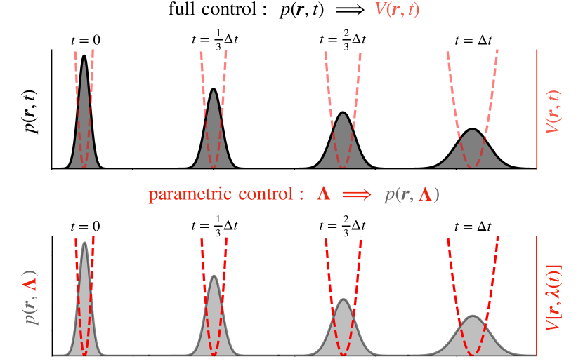
Figure 1: Comparing full control and parametric control. Full control (top) assumes complete control of the probability distribution $p(\boldsymbol{r},t)$ (shaded) which can be optimally driven between the endpoints by a potential $V(\boldsymbol{r},t)$ (red dashed curves). Parametric control (bottom) adjusts a finite number of control parameters $\boldsymbol{\lambda}(t)$ according to a protocol $\boldsymbol{\Lambda}$ between specified endpoints, thereby driving the probability distribution $p(\boldsymbol{r},\boldsymbol{\Lambda})$.

For either full or parametric control, the exact minimum-dissipation protocol is known if the probability distribution is Gaussian Schmiedl and Seifert (2007); Abiuso et al. (2022); Blaber and Sivak (2022a). These exact solutions provide a glimpse into the properties of optimal control processes. For example, just like the finite-time thermodynamic control described previously, the minimum-dissipation protocol has discontinuous changes in control parameters at the start and end of the protocol but remains continuous between these endpoints Schmiedl and Seifert (2007). These discontinuities are present even for underdamped dynamics Gomez-Marin et al. (2008). The control-parameter jumps have been observed in a number of different systems Gomez-Marin et al. (2008); Then and Engel (2008); Esposito et al. (2010a) and are now well understood and have been shown to be a general feature Blaber et al. (2021).

For more general solutions under full control, the study of minimum-dissipation protocols can be mapped onto a problem of optimal-transport theory, a well developed branch of mathematics for which there exist numerous algorithms and methods for determining the optimal-transport map Villani (2009); Santambrogio (2015). The connection between minimum-dissipation protocols and optimal-transport theory was first shown in Ref. Aurell et al., 2011 for overdamped dynamics: the protocol that minimizes dissipation when driving a system obeying overdamped Fokker-Planck dynamics between specified initial and final distributions is governed by the Wasserstein distance Zhang (2019); Nakazato and Ito (2021); Dechant (2022); Miangolarra et al. (2022) and the Benamou-Brenier formula Benamou and Brenier (2000). This technique eventually led to new fundamental lower bounds on the average work required for finite-time information erasure Proesmans et al. (2020a, b). Initially only applicable to overdamped dynamics, the connections between optimal-transport theory and minimum-dissipation protocols have recently been shown for discrete-state and quantum systems Dechant (2022); Dechant et al. (2022); Yoshimura et al. (2022); Zhong and DeWeese (2022); Van Vu and Saito (2023a); Van Vu and Saito (2023b).

General solutions for parametric control are typically difficult to determine, although recent progress has been made towards exact solutions for general systems building off of optimal-transport Zhong and DeWeese (2022) or advanced numerical techniques Then and Engel (2008); Gingrich et al. (2016); Engel et al. (2022). Although exact solutions are convenient where possible, the determination of minimum-dissipation protocols can be considerably simplified through approximate methods. Inspired by a diagram presented in Ref. Bonança and Deffner, 2018, we schematically show in Fig. 2 the limits where minimum-dissipation protocols are known.

Linear-response theory can be used to determine the minimum-dissipation protocol for weak perturbations and performs relatively well at any driving speed and beyond its strict range of validity Kamizaki et al. (2022); Bonança and Deffner (2018). For slow control, the thermodynamic-geometry framework has been generalized to stochastic thermodynamic systems Crooks (2007); Sivak and Crooks (2016) and has been used to explore a diverse set of model systems Sivak and Crooks (2016); Blaber and Sivak (2020a); Deffner and Bonança (2020); Zulkowski et al. (2012); Bonança and Deffner (2014); Zulkowski and DeWeese (2015a, b); Large and Sivak (2019); Lucero et al. (2019); Rotskoff and Crooks (2015); Rotskoff et al. (2017); Louwerse and Sivak (2022); Frim and DeWeese (2022a, b), including DNA-pulling experiments Tafoya et al. (2019) and free-energy estimation Blaber and Sivak (2020b). In the opposite limit of fast control, minimum-dissipation protocols are describe by short-time efficient protocols Blaber et al. (2021), which can be combined with the thermodynamic-geometry framework to design interpolated protocols that perform well at any driving speed Blaber and Sivak (2022b). Leveraging known solutions from optimal-transport theory, strong control can be described by the strong-trap approximation, yielding explicit solutions for minimum-dissipation protocols Blaber and Sivak (2022a).

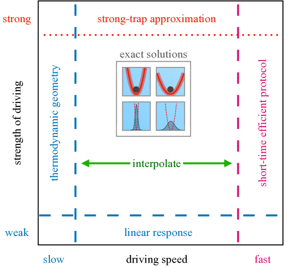
Figure 2: The space of thermodynamic control. Horizontal axis is the driving speed from slow to fast, and the vertical axis is the strength of driving from weak to strong. Linear-response theory is applicable to weak and slow driving (blue), and can be simplified to a thermodynamic-geometry framework for slow driving. Short-time efficient protocols are valid for fast driving (purple) and can be combined with thermodynamic geometry to bridge the space between slow and fast with interpolated protocols (green). The strong-trap approximation (red) is only valid for overdamped dynamics, with region of applicability schematically indicated by a distinct dotted line. Exact solutions for Gaussian distributions serve as a window into the properties of minimum-dissipation protocols and are valid at any driving speed or strength of driving.

There are a number of related topics which are not covered in this review, such as optimal control of heat enginesHolubec and Ryabov (2021) (including optimal cycles Ma et al. (2018a); Zhang (2020); Abiuso and Perarnau-Llobet (2020); Frim and DeWeese (2022b, a); Chen (2022) and efficiency at maximum power Curzon and Ahlborn (1975); Van den Broeck (2005); Schmiedl and Seifert (2008); Esposito et al. (2009); Esposito et al. (2010b); Brandner et al. (2015); Proesmans et al. (2016); Shiraishi et al. (2016); Ma et al. (2018b, 2020); Miller and Mehboudi (2020); Brandner and Saito (2020); Miangolarra et al. (2021, 2022); Watanabe and Minami (2022)) and optimal control in quantum thermodynamics (including thermodynamic geometry Acconcia et al. (2015); Zulkowski and DeWeese (2015b); Scandi and Perarnau-Llobet (2019); Deffner and Bonança (2020) and shortcuts to adiabaticity Takahashi (2017); Guéry-Odelin et al. (2019, 2022)).

This review is organized as follows: we begin with examples of both experimental and theoretical model systems in section II, followed by a brief introduction to stochastic thermodynamics of heat, work, and entropy production in section III. Section IV reviews recent progress exploiting optimal-transport theory to determine minimum-dissipation protocols under full control, yielding explicit solutions for the minimum-dissipation protocol under a strong-trap approximation in section IV.2 and allowing for constrained final control parameters in section IV.3. Section V reviews parametric control, focusing on approximation methods in the fast (section V.1), weak (section V.2), and slow (section V.3) limits. Applications to free-energy estimation are discussed in section VI before comparing the performance of designed protocols in section VII and finally concluding in section VIII with a perspective and outlook for the study of optimal control in stochastic thermodynamics.

II Model systems

In this section we provide a brief introduction to a few paradigmatic model systems that motivate and guide the study of optimal control in stochastic thermodynamics. As discussed in section I, the growth of stochastic thermodynamics coincides with the advent of new experimental techniques used to manipulate and measure single-molecule biophysical systems Toyabe et al. (2011, 2012); Kawaguchi et al. (2014); Svoboda et al. (1993); Svoboda and Block (1994); Kojima et al. (1997); Hunt et al. (1994); Greenberg et al. (2016); Laakso et al. (2008); Norstrom et al. (2010); Nagy et al. (2013). First and foremost among these techniques are laser optical tweezers Bustamante et al. (2021); Polimeno et al. (2018); Moffitt et al. (2008) which can be used to trap microscopic Brownian systems.

The simplest experimental apparatus for studying stochastic thermodynamics is that of a microscopic bead trapped in an optical potential. From a theoretical perspective, this system is well approximated by continuous overdamped Brownian motion in a quadratic constraining potential. In these experiments, the center and stiffness of the trapping potential can be dynamically controlled to manipulate the system. With the use of feedback control, this experimental apparatus can be augmented to realize a virtual constraining potential of any form Kumar and Bechhoefer (2018, 2019); Gavrilov and Bechhoefer (2017) and can, for example, be used to study fundamental bounds on information processing through bit erasure Jun et al. (2014); Gavrilov and Bechhoefer (2016).

Microscopic beads trapped by laser optical tweezers can be attached to biopolymers to probe their properties. For example, dual-trap optical tweezers can be used to fold and unfold DNA or RNA hairpins by modulating the separation between the trapping potentials (Fig. 3 a).Liphardt et al. (2002); Collin et al. (2005); Bustamante et al. (2000, 2003); Woodside et al. (2006); Neupane et al. (2017) Monitoring the position of the probe beads provides insight into the properties of the indirectly observed biopolymers. The simplest model representing this process is that of a driven barrier crossing Neupane et al. (2015), where a Brownian system is dynamically driven over an energy barrier by a time-varying quadratic trapping potential (Fig. 3 d).Sivak and Crooks (2016); Blaber and Sivak (2022b)

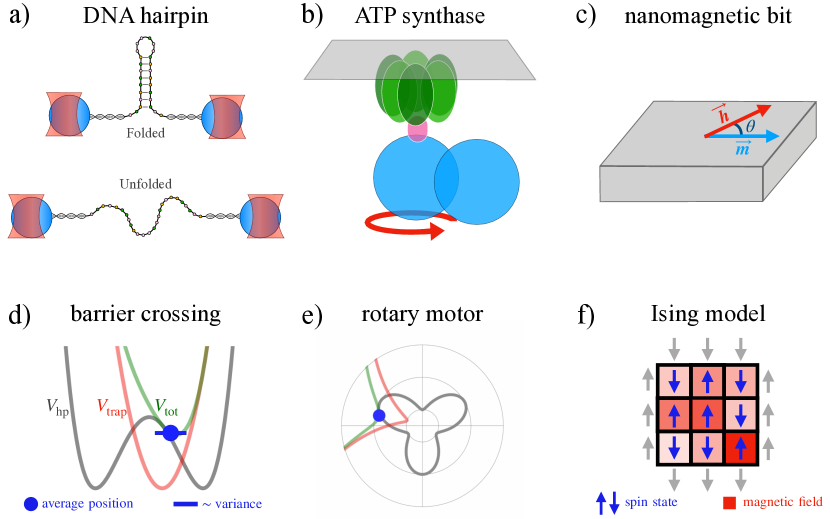
Figure 3: Model systems typical of stochastic thermodynamic control (top): a) DNA hairpin driven between folded and unfolded states by laser optical tweezers, b) ATP synthase driven by a magnetic trapping potential, c) nanomagnetic bit driven by an external magnetic field. Simplified theoretical descriptions (bottom) of the model systems in the top row: d) symmetric barrier-crossing model, e) Brownian rotary motor model, and f) nine-spin Ising model with independent magnetic fields applied to each spin.

Magnetic traps can be used to probe the F1 component of the rotary motor ATP synthase (Fig. 3 b),Toyabe et al. (2011, 2012); Kawaguchi et al. (2014) which is driven periodically to synthesize ATP, an essential and portable energy source for the cell. Once again, microscopic beads are used to probe the properties of the molecular machine and can be dynamically driven (Fig. 3 e); however, the control differs from driven barrier crossing in that the driving is periodic.

As a final example, consider a nanomagnetic bit characterized by its spin state or average magnetization (Fig. 3 c). By applying an external magnetic field, the system state can be driven from all spin-down to all spin-up, reversing the magnetization and resulting in a bit flip Hong et al. (2016). This type of system is typically modeled with a discrete state space, e.g., the Ising model (Fig. 3 f), and optimal control of this system has been investigated Rotskoff and Crooks (2015); Rotskoff et al. (2017); Louwerse and Sivak (2022). Due to the discrete state space, the properties of optimal control can differ from those for a system with a continuous state space.

Throughout this review we will use the model system of overdamped driven barrier crossing previously studied in Ref. Blaber and Sivak, 2022b in order to give some intuition and examples for optimal control. The model consists of an overdamped Brownian particle in a double-well potential (symmetric for simplicity) constrained and driven by a quadratic trapping potential (Fig. 3 d). This system represents a simplified model of hairpin pulling experiments and Landauer erasure Blaber and Sivak (2022b); Proesmans et al. (2020a, b). The two-state nature of the system is also representative of activated processes such as chemical reactions, and the barrier crossing mimics the main features of experiments performed on ATP synthase, whose dynamics can be approximated as a series of barrier crossings Kawaguchi et al. (2014); Lucero et al. (2019); Gupta et al. (2022). This model is also typical of steered molecular-dynamics simulations, which use a time-dependent quadratic potential to drive reactions Park et al. (2003); Park and Schulten (2004); Dellago and Hummer (2014).

The total potential $V_{\rm tot}[x,x^{\rm c}(t),k(t)]=V_{\rm land}[x]+V_{\rm trap}[x,x^{\rm c}(t),k(t)]$ is the sum of the static hairpin potential $V_{\rm land}[x]$ and time-dependent trap potential $V_{\rm trap}[x,x^{\rm c}(t),k(t)]$ (shown schematically in Fig. 3d). The hairpin potential is modeled as a static double well (symmetric for simplicity) with the two minima at $x=0$ and $x=\Delta x_{\rm m}$ representing the folded and unfolded states Neupane et al. (2015, 2017); Woodside et al. (2006); Sivak and Crooks (2016),

$$V_{\rm land}(x)=E_{\rm B}\left[\left(\frac{2x-\Delta x_{\rm m}}{\Delta x_{\rm m}}\right)^{2}-1\right]^{2}\ ,$$ (1)

for barrier height $E_{\rm B}$, distance $x_{\rm m}$ from the minimum to barrier, and distance $\Delta x_{\rm m}=2x_{\rm m}$ between the minima. The system is driven by a quadratic trap

$$V_{\rm trap}[x,x^{\rm c}(t),k(t)]=\frac{k(t)}{2}\left[x^{\rm c}(t)-x\right]^{2}\ ,$$ (2)

with time-dependent stiffness $k(t)$ and center $x^{\rm c}(t)$.

III Thermodynamics

In this review we focus on thermodynamics at the distribution level, which is generally described by dynamics of the form

$$\frac{\partial p(\boldsymbol{r},t)}{\partial t}=\mathcal{L}[\boldsymbol{r},t]\ p(\boldsymbol{r},t)\ ,$$ (3)

governing the time evolution of a nonequilibrium probability distribution $p(\boldsymbol{r},t)$ over position vector $\boldsymbol{r}$ at time $t$ according to the time-evolution operator $\mathcal{L}[\boldsymbol{r},t]$.

Continuous-space stochastic systems are described by the Fokker-Planck equation, which for overdamped dynamics has the time-evolution operator

$$\mathcal{L}[\boldsymbol{r},t]=\nabla\cdot\boldsymbol{v}(\boldsymbol{r},t)+\boldsymbol{v}(\boldsymbol{r},t)\cdot\nabla\ ,$$ (4)

for mean local velocity Nakazato and Ito (2021)

$$\boldsymbol{v}(\boldsymbol{r},t)\equiv-D\nabla\left[\beta V_{\rm tot}(\boldsymbol{r},t)+\ln p(\boldsymbol{r},t)\right]\ ,$$ (5)

total potential $V_{\rm tot}$, diffusivity $D$, and $\beta\equiv(k_{\rm B}T)^{-1}$ for temperature $T$ and Boltzmann’s constant $k_{\rm B}$. For a discrete-state system, $\mathcal{L}[\boldsymbol{r},t]$ is the transition rate matrix. For the example of driven barrier crossing, the total potential includes both the hairpin and trapping potential, and the time dependence arises from dynamic changes in the trap center and stiffness which drive the system over the barrier.

The average system energy is

$$U=\int\mathrm{d}\boldsymbol{r}~{}V(\boldsymbol{r},t)p(\boldsymbol{r},t)\ ,$$ (6)

and the rate of change in energy is

$$\frac{\mathrm{d}U}{\mathrm{d}t}=\int\mathrm{d}\boldsymbol{r}\left[\frac{\partial V(\boldsymbol{r},t)}{\partial t}p(\boldsymbol{r},t)+\frac{\partial p(\boldsymbol{r},t)}{\partial t}V(\boldsymbol{r},t)\right]\ .$$ (7)

The first term quantifies work $W$ done on the system by an external agent controlling the potential $V(\boldsymbol{r},t)$ (e.g., an experimentalist dynamically driving a trapping potential) and the second quantifies heat flow $Q$ into the system from changes in the system distribution $p(\boldsymbol{r},t)$ (e.g., the system responding and relaxing towards a new equilibrium distribution in response to movement of the center and stiffness of the trapping potential):

$$\dot{W} \equiv\int\mathrm{d}\boldsymbol{r}~{}\frac{\partial V(\boldsymbol{r},t)}{\partial t}p(\boldsymbol{r},t)\ ,$$ (8)

$$\dot{Q} \equiv\int\mathrm{d}\boldsymbol{r}~{}\frac{\partial p(\boldsymbol{r},t)}{\partial t}V(\boldsymbol{r},t)\ .$$ (9)

Throughout, a dot above a variable denotes the rate of change with respect to time. Substituting (8) and (9) into (7) gives the first law of thermodynamics: any change in system energy equals work and heat flows into the system.

Optimal control in thermodynamics is often discussed in terms of minimizing either entropy production or excess work incurred during the protocol. The entropy production as defined in this review will be used for periodic systems (e.g., ATP synthase), and when we have full control over the distribution (section IV). The excess work is used for parametric control (section V) and model systems like DNA hairpins and nanomagnetic bits which are driven between control-parameter endpoints rather than periodically.

To understand these two concepts, consider the nonequilibrium free energy

$$F_{\rm neq} \equiv U-\beta^{-1}S$$ (10a)

$$=\int\mathrm{d}\boldsymbol{r}~{}\left[V(\boldsymbol{r},t)\,p(\boldsymbol{r},t)+\beta^{-1}\,p(\boldsymbol{r},t)\ln p(\boldsymbol{r},t)\right]\ ,$$ (10b)

for dimensionless entropy

$$S\equiv-\int\mathrm{d}\boldsymbol{r}~{}p(\boldsymbol{r},t)\ln p(\boldsymbol{r},t)\ .$$ (11)

If the probabilities in (10b) are equilibrium distributions, then the nonequilibrium free energy reduces to the equilibrium free energy $F_{\rm eq}$. For an isothermal process the rate of change in free energy is

$$\frac{\mathrm{d}F_{\rm neq}}{\mathrm{d}t} =\frac{\mathrm{d}U}{\mathrm{d}t}-\beta^{-1}\frac{\mathrm{d}S}{\mathrm{d}t}\ ,$$ (12a)

$$=\dot{W}+\dot{Q}-\beta^{-1}\frac{\mathrm{d}S}{\mathrm{d}t}\ ,$$ (12b)

$$=\dot{W}-\beta^{-1}\dot{S}_{\rm prod}\ .$$ (12c)

The dimensionless entropy production is

$$\dot{S}_{\rm prod} \equiv\frac{\mathrm{d}S}{\mathrm{d}t}+\frac{\mathrm{d}S_{\rm env}}{\mathrm{d}t}$$ (13a)

$$=\frac{\mathrm{d}S}{\mathrm{d}t}-\beta\dot{Q}$$ (13b)

$$\geq 0\ ,$$ (13c)

for environmental entropy $S_{\rm env}$. Equation (13c) follows from the second law of thermodynamics. Importantly, this definition of entropy production only accounts for dissipation during the protocol, so if the system is not in equilibrium at the end of the protocol, additional energy may be dissipated into the environment during subsequent relaxation.

A measure of energy dissipation which accounts for relaxation to equilibrium even after the protocol terminates is the excess work $W_{\rm ex}\equiv W-\Delta F_{\rm eq}$, the amount of work done in excess of the equilibrium free-energy difference. The excess work and entropy production are related by

$$W_{\rm ex}=\Delta F_{\rm neq}-\Delta F_{\rm eq}+\beta^{-1}\Delta S_{\rm prod}\ ,$$ (14)

for net entropy production $\Delta S_{\rm prod}\equiv\int_{0}^{\Delta t}\mathrm{d}t\,\dot{S}_{\rm prod}$, nonequilibrium free-energy difference $\Delta F_{\rm neq}$ between the initial $p(\boldsymbol{r},0)$ and final $p(\boldsymbol{r},\Delta t)$ distributions, and equilibrium free-energy difference $\Delta F_{\rm eq}$ between the initial and final equilibrium distributions.

Equation (14) clarifies the distinction between entropy production and excess work: if both the initial and final states of the system are at equilibrium, the two quantities are equal, otherwise the difference between the two equals the difference between the nonequilibrium and equilibrium free-energy changes. If the system is allowed to relax to equilibrium, then this excess energy is dissipated into the environment, resulting in additional entropy production not accounted for in the present definition (13a), so that the total entropy production for such a process is (13a) plus the entropy production from the subsequent relaxation. In contrast, the excess work always includes the energy dissipated into the environment from the system relaxing towards equilibrium after the protocol terminates. Essentially, quantifying dissipation by the entropy production in (13a) assumes one can harness the nonequilibrium free energy at the conclusion of the protocol to perform a useful task (generally true for periodically driven systems like ATP synthase), while excess work quantifies dissipation when all the excess free energy is dissipated into the environment after the protocol terminates (generally true for two-state barrier crossings like hairpin experiments).

IV Full control

For continuous-state systems, complete control over the shape of the potential $V(\boldsymbol{r},t)$ grants full control over the probability distribution $p(\boldsymbol{r},t)$, which can considerably simplify the optimization process and allows us to exploit known results from optimal-transport theory Aurell et al. (2011); Nakazato and Ito (2021); Ito (2023). Optimal transport describes the most efficient methods to move mass (e.g., a pile of sand) from one location to another; this is useful for describing methods that minimize dissipation in transporting probability from an initial to a final distribution Villani (2009).

Since the final distribution is constrained, the energy dissipated into the environment throughout the protocol is determined by the average entropy produced in driving from initial probability distribution $p(\boldsymbol{r},0)$ to final probability distribution $p(\boldsymbol{r},\Delta t)$ as Nakazato and Ito (2021)

$$\Delta S_{\rm prod}=\frac{1}{D}\int_{0}^{\Delta t}\mathrm{d}t\ \langle\boldsymbol{v}(\boldsymbol{r},t)\cdot\boldsymbol{v}(\boldsymbol{r},t)\rangle\ .$$ (15)

Angle brackets $\langle\cdots\rangle$ denote an average over $p(\boldsymbol{r},t)$.

Expressing the entropy production in this form makes precise the connections between optimal-transport theory and minimum-dissipation protocols. In optimal-transport theory a common measure of the distance between two distributions is the $L_{2}$-Wasserstein distance, defined in the Benamou and Brenier dual representation as Benamou and Brenier (2000)

$$\mathcal{W}(p_{0},p_{\Delta t})^{2}\equiv\min_{v}\int_{0}^{\Delta t}\mathrm{d}t\ \langle\boldsymbol{v}(\boldsymbol{r},t)\cdot\boldsymbol{v}(\boldsymbol{r},t)\rangle\ .$$ (16)

Therefore, the entropy production is bounded by the squared $L_{2}$-Wasserstein distance between initial ($p_{0}$) and final ($p_{\Delta t}$) probability distributions Nakazato and Ito (2021):

$$\Delta S_{\rm prod}\geq\frac{\mathcal{W}\left(p_{0},p_{\Delta t}\right)^{2}}{D\Delta t}\ .$$ (17)

This allows us to exploit existing procedures from optimal-transport theory to determine protocols that minimize entropy production Villani (2009); Santambrogio (2015). Notably, the exact solution is known in two situations: one-dimensional systems and Gaussian probability distributions (section IV.1).

Extending minimum-dissipation full control and the connections to optimal-transport theory to more general forms of dynamics (e.g., discrete state spaces) is a rapidly advancing area of active research.Dechant (2022); Dechant et al. (2022); Yoshimura et al. (2022); Zhong and DeWeese (2022); Van Vu and Saito (2023a); Van Vu and Saito (2023b)

IV.1 Exact solutions

For a one-dimensional system $\boldsymbol{r}=x$, the entropy production (15) of the optimal-transport process can be simplified considerably as Aurell et al. (2011); Abreu and Seifert (2011); Zhang (2019, 2020); Proesmans et al. (2020a, b)

$$\Delta S_{\rm prod}\geq\frac{1}{D\Delta t}\int_{0}^{1}\mathrm{d}y\left[\mathcal{Q}_{\rm f}(y)-\mathcal{Q}_{\rm i}(y)\right]^{2}\ ,$$ (18)

where $\mathcal{Q}_{\rm f}$ and $\mathcal{Q}_{\rm i}$ are the final and initial quantile functions (inverse cumulative distribution functions) Blaber and Sivak (2022b). The entropy production is minimized if the quantiles are linearly driven between their fixed initial and final values Zhang (2019, 2020); Proesmans et al. (2020a, b); from this the probability distribution can be computed, and then the Fokker-Planck equation inverted to determine the potential $V_{\rm tot}(x,t)$ to be applied to achieve the control that minimizes the entropy production:

$$V_{\rm tot}(x,t)=-\beta^{-1}\ln p(x,t)+(\beta D)^{-1}\int_{-\infty}^{x}\mathrm{d}x^{\prime}~{}\frac{\int_{-\infty}^{x^{\prime}}\mathrm{d}x^{\prime\prime}~{}\frac{\partial p(x^{\prime\prime},t)}{\partial t}}{p(x^{\prime},t)}\ .$$ (19)

Although this calculation is often analytically intractable, it is straightforward to compute numerically for any probability distribution.

If the initial and final distributions are Gaussian, $p(\boldsymbol{r},t)=\mathcal{N}(\mu_{t},\Sigma_{t})$ for time-dependent mean $\mu_{t}$ and covariance $\Sigma_{t}$, the entropy-production bound (17) is Olkin and Pukelsheim (1982); Dechant and Sakurai (2019); Abiuso et al. (2022)

$$\Delta S_{\rm prod}\geq\frac{1}{D\Delta t}\bigg{\{}\Delta\boldsymbol{\mu}^{2}+{\rm Tr}\left[\Sigma_{0}+\Sigma_{\Delta t}-2(\Sigma_{\Delta t}^{\frac{1}{2}}\Sigma_{0}\Sigma_{\Delta t}^{\frac{1}{2}})^{\frac{1}{2}}\right]\bigg{\}}\ ,$$ (20)

with subscripts $0$, $t$, and $\Delta t$ respectively denoting the initial, time-dependent, and final values of the corresponding variable. Equality is achieved and the entropy production is minimized when following the optimal-transport map between the initial and final distributions, which for Gaussian distributions is completely specified by the mean and covariance:

$$\boldsymbol{\mu}_{t} =\boldsymbol{\mu}_{0}+\Delta\boldsymbol{\mu}\frac{t}{\Delta t}$$ (21a)

$$\Sigma_{t} =\left[\left(1-\frac{t}{\Delta t}\right)I+\frac{t}{\Delta t}C\right]\Sigma_{0}\left[\left(1-\frac{t}{\Delta t}\right)I+\frac{t}{\Delta t}C\right]\ .$$ (21b)

Here $\Delta\boldsymbol{\mu}\equiv\boldsymbol{\mu}_{\Delta t}-\boldsymbol{\mu}_{0}$ is the total change in mean position, $I$ is the identity matrix, and $C\equiv\Sigma_{\Delta t}^{\frac{1}{2}}(\Sigma_{\Delta t}^{\frac{1}{2}}\Sigma_{0}\Sigma_{\Delta t}^{\frac{1}{2}})^{-\frac{1}{2}}\Sigma_{\Delta t}^{\frac{1}{2}}$ reduces in 1D to the ratio of final and initial standard deviations. If the covariance matrix $\Sigma$ is diagonal, then (21b) implies

$$\Sigma_{t}^{\frac{1}{2}} =\Sigma_{0}^{\frac{1}{2}}+\Delta\Sigma^{\frac{1}{2}}\frac{t}{\Delta t}\ ,$$ (22)

with $\Delta\Sigma^{\frac{1}{2}}\equiv\Sigma^{\frac{1}{2}}_{\Delta t}-\Sigma^{\frac{1}{2}}_{0}$. Thus for diagonal covariance the optimal-transport process linearly drives the standard deviation between its endpoint values. For a detailed description of minimum-dissipation protocols for general multidimensional Gaussian distributions see Ref. Abiuso et al., 2022.

In both solvable cases (1D and Gaussian) the general design principle is that the minimum-dissipation protocol linearly drives the quantiles between specified initial and final values. Linearly driving the quantiles of the probability distribution can be used as a guiding principle for designing more general minimum-dissipation protocols and arises independently for parametric control Blaber and Sivak (2022b).

IV.2 Strong-trap approximation

In this section we review how to exploit the known full-control solution for Gaussian distributions in order to design minimum-dissipation protocols for strong trapping potentials on any arbitrary underlying energy landscape, initially described in Ref. Blaber and Sivak, 2022a.

We assume that the total potential $V_{\rm tot}[\boldsymbol{r},\boldsymbol{r}_{\rm c}(t),K(t)]=V_{\rm land}(\boldsymbol{r})+V_{\rm trap}[\boldsymbol{r},\boldsymbol{r}_{\rm c}(t),K(t)]$ can be separated into a time-independent component $V_{\rm land}(\boldsymbol{r})$ (the underlying energy landscape) and a quadratic trapping potential

$$V_{\rm trap}[\boldsymbol{r},\boldsymbol{r}_{\rm c}(t),K(t)]=\frac{1}{2}\left[\boldsymbol{r}-\boldsymbol{r}_{\rm c}(t)\right]^{\top}K(t)\left[\boldsymbol{r}-\boldsymbol{r}_{\rm c}(t)\right]\ .$$ (23)

The position of the system is denoted by the vector $\boldsymbol{r}$, $K$ is the symmetric stiffness matrix, and superscript $\top$ is the vector transpose. For a strong trapping potential, the time-independent component can be expanded up to second order about the mean particle position $\boldsymbol{\mu}$:

$$V_{\rm land}(\boldsymbol{r})\approx V_{\rm land}(\boldsymbol{\mu})+(\boldsymbol{r}-\boldsymbol{\mu})^{\top}\nabla V_{\rm land}(\boldsymbol{\mu})+\frac{1}{2}(\boldsymbol{r}-\boldsymbol{\mu})^{\top}\nabla\nabla^{\top}V_{\rm land}(\boldsymbol{\mu})(\boldsymbol{r}-\boldsymbol{\mu})\ .$$ (24)

Under these assumptions, the probability distribution can be approximated as Gaussian, $p(\boldsymbol{r},t)\approx\mathcal{N}(\boldsymbol{\mu}_{t},\Sigma_{t})$. Since the distribution is Gaussian we can use the results described by (21a) and (21b).

To achieve the mean and covariance of (21a) and (21b), the trap center and stiffness must respectively satisfy

$$\boldsymbol{\lambda}_{t}= \boldsymbol{\mu}_{t}+K_{t}^{-1}\left[\frac{\Delta\boldsymbol{\mu}}{\beta D\Delta t}+\nabla V_{\rm land}(\boldsymbol{\mu}_{t})\right]\ ,$$ (25a)

$$K_{t}= \frac{1}{\beta}\Sigma_{t}^{-1}-\frac{1}{\beta D}\int_{0}^{\infty}\mathrm{d}\nu\ e^{-\nu\Sigma_{t}}\frac{\mathrm{d}\Sigma_{t}}{\mathrm{d}t}e^{-\nu\Sigma_{t}}-\nabla\nabla^{\top}V_{\rm land}(\boldsymbol{\mu}_{t})\ .$$ (25b)

If $\Sigma$ is diagonal, then $\Sigma_{t}$ is given by (22), the integral in (25b) can be evaluated, and the trap stiffness obeys

$$K_{t} =\nabla\nabla^{\top}V_{\rm land}(\boldsymbol{\mu}_{t})+\left(\frac{1}{\beta}I-\frac{\Delta\Sigma^{\frac{1}{2}}}{2\beta D\Delta t}\right)\Sigma_{t}^{-1}.$$ (26)

Equations (25a) and (25b) are explicit equations that minimize dissipation at any driving speed provided the trap is sufficiently strong. We emphasize that explicit solutions for the minimum-dissipation protocol are rarities; typically solutions require numerically solving differential equations or inverting the Fokker-Planck equation Aurell et al. (2011); Proesmans et al. (2020a, b).

For our example system of driven barrier crossing with equal initial and final covariance, the protocol designed by (25a) slows down movement of the trap center as it crosses the barrier to compensate for the force due to the hairpin potential, and (27) tightens the trap as it crosses the barrier in order to counteract the negative curvature of the hairpin potential. Slowing down and tightening the trapping potential as the system crosses a barrier appears to be a general feature and results independently from other approximation methods Blaber and Sivak (2022b); Blaber and Sivak (2022a).

To achieve periodic driving we constrain the final covariance matrix after one period (during which the mean completes one rotation) to equal the initial. To minimize dissipation, the standard deviation is linearly changed between the endpoints (21b), implying for a periodic system that the standard deviation (and hence covariance) remains unchanged throughout the protocol. This is achieved when the effective stiffness is constant, i.e.,

$$K_{t}=K_{0}+\nabla\nabla^{\top}V_{\rm land}(\boldsymbol{\mu}_{0})-\nabla\nabla^{\top}V_{\rm land}(\boldsymbol{\mu}_{t})\ .$$ (27)

If in each rotation the mean travels a distance $\Delta\boldsymbol{\mu}_{\rm rot}$ in time $\Delta t_{\rm rot}$, the resultant entropy production is

$$\Delta S_{\rm prod}=\frac{\Delta\boldsymbol{\mu}_{\rm rot}^{2}}{D\Delta t_{\rm rot}}\ ,$$ (28)

that of an overdamped system moving at constant velocity against viscous Stokes drag; i.e., the minimum-dissipation protocol has perfect Stokes efficiency Wang and Oster (2002).

IV.3 Constrained final control parameters

The techniques described in section IV minimize the entropy production for constrained final distributions. Constraining the final distribution allows us to describe periodically driven systems like models inspired by ATP synthase; however, often the end state is instead constrained by the final control-parameter values. For example, in hairpin experiments the end state is typically defined by the trap separation, and the system is typically allowed to equilibrate between subsequent unfolding/folding protocols. Since the system is allowed to equilibrate between protocols, any excess energy remaining at the end of the protocol is dissipated as heat into the environment, and the entropy production as defined by (13a) does not equal the total dissipation.

In this case the relevant thermodynamic quantity is the work (14),

$$W=\Delta F_{\rm neq}+\Delta S_{\rm prod}\ ,$$ (29)

which accounts for the excess free energy dissipated into the environment after the protocol terminates. Work can be minimized by optimizing over the final distribution subject to constrained final control-parameter values Blaber and Sivak (2022a); Blaber and Sivak (2022b). In general this minimization must be performed numerically, which is straightforward for one-dimensional systems, but becomes computationally intensive for higher-dimensional systems.

For the special case of Gaussian distributions, the optimization procedure simplifies considerably since optimizing over a distribution reduces to optimizing over means and covariances. The average work for the minimum-dissipation protocol in the strong-trap approximation is Blaber and Sivak (2022a)

$$W= \frac{1}{2}{\rm Tr}\left\{K\left[\Sigma+(\boldsymbol{\mu}-\boldsymbol{\lambda})(\boldsymbol{\mu}-\boldsymbol{\lambda})^{\top}\right]\right\}_{0}^{\Delta t}+V_{\rm land}(\boldsymbol{\mu})\big{|}_{0}^{\Delta t}+\frac{1}{2}{\rm Tr}\left[\nabla\nabla^{\top}V_{\rm land}(\boldsymbol{\mu})\Sigma\right]_{0}^{\Delta t}+\beta^{-1}\Delta S_{\rm prod}^{\rm min}\ ,$$ (30)

with ${\rm Tr}$ the trace and $\Delta S_{\rm prod}^{\rm min}$ the lower bound in (20).

To find the protocol that minimizes work for constrained final control parameters, we minimize (30) with respect to the final mean $\mu_{\Delta t}$ and covariance $\Sigma_{\Delta t}$, for fixed final trap center $\boldsymbol{\lambda}_{\Delta t}$ and stiffness $K_{\Delta t}$. For a flat energy landscape (for which the strong-trap approximation is exact) the optimal mean and covariance can be solved analytically; e.g., for equal initial and final covariance, the final mean is

$$\boldsymbol{\mu}_{\Delta t}=\boldsymbol{\mu}_{0}+\left(\frac{2K^{-1}}{\beta D\Delta t}+I\right)^{-1}[\boldsymbol{\lambda}_{\Delta t}-\boldsymbol{\mu}_{0}]\ .$$ (31)

In some more general cases (e.g., energy landscapes represented by low-order polynomials), (30) can also be minimized analytically, and in general can be solved numerically with relative ease.

V Parametric control

While full-control solutions are convenient when possible, many applications do not permit sufficient control to fully constrain the probability distribution throughout the entire protocol. In such cases the controller is constrained by a finite set of control parameters $\boldsymbol{\lambda}(t)$ which can be used to drive the system. Since there are insufficient control parameters to fully control the probability distribution, the endpoints of the protocol are constrained by the control-parameter values rather than the distribution. Therefore, we focus on optimizing the excess work, which is an accurate measure of dissipation provided the system equilibrates after the protocol terminates.

In this section we assume the control is the result of time-dependent control parameters $\boldsymbol{\lambda}(t)$, in which case the excess work (8) is

$$\langle W_{\rm ex}\rangle_{\Lambda}~{}=-\int_{0}^{\Delta t}{\rm d}t~{}\langle\delta{\bf f}^{\top}(t)\rangle_{\Lambda}\dot{\boldsymbol{\lambda}}(t)\ ,$$ (32)

where we have defined the conjugate force ${\bf f}\equiv-\partial V_{\rm tot}/\partial\boldsymbol{\lambda}$ to express the work explicitly in terms of the control parameters, and $\delta$ denotes a difference from the equilibrium average. In this section we denote a nonequilibrium average (dependent on the entire protocol history) as $\langle\cdot\rangle_{\Lambda}$ and an equilibrium average (at the current control parameter value $\boldsymbol{\lambda}(t)$) as $\langle\cdot\rangle_{\boldsymbol{\lambda}(t)}$. Since the control-parameter protocol is externally specified, the only unknown is $\langle\delta{\bf f}^{\top}(t)\rangle_{\Lambda}$. This quantity is particularly difficult to deal with since the nonequilibrium average depends on the entire protocol history.

For example, Ref. Schmiedl and Seifert, 2007 showed that—even in one dimension—optimization requires solving the nonlocal Euler-Lagrange equation. Therefore, there are very few cases where the minimum-work protocol can be determined analytically. Promising approaches for obtaining general solutions include optimal-transport theory with limited control Zhong and DeWeese (2022) and advanced numerical techniques Then and Engel (2008); Gingrich et al. (2016); Engel et al. (2022).

The minimum-work protocol can be determined exactly for a Brownian particle in a harmonic trap, in which case the optimal protocol, originally derived in one dimension Schmiedl and Seifert (2007), is identical to the full-control solution for Gaussian distributions described in section IV.3. This exact solution serves as a window into the properties of minimum-dissipation protocols and gives us considerable insight into what to expect from optimized protocols: e.g., the minimum-dissipation protocols have control-parameter jumps at the start and end but remain continuous in between.

Although exact solutions are nice when possible, since general solutions are intractable we turn to approximate methods to gain insight into the general properties of minimum-dissipation protocols. The first approximation has already been described in section IV.2 and is valid for strong trapping potentials applied to overdamped systems Blaber and Sivak (2022a). In the following sections, we fill in the remaining limits of fast, weak, and slow control in order to describe optimal control for any system with any given control parameters and design interpolated protocols.

V.1 Fast control

Until recently, although it was generally suspected, it was not definitively known whether the jumps in the minimum-dissipation protocols are a general feature. By taking the fast-driving limit, it has been shown that the minimum-dissipation protocol is a step function, jumping from and to specified initial and final control-parameter endpoints to spend the entire intervening protocol duration at the control-parameter values that maximize the short-time power savings.Blaber et al. (2021) We refer to the minimum-dissipation protocols in the fast limit as short-time efficient protocols, or STEP.

In the fast limit, the excess work approaches that of an instantaneous protocol, which spends no time relaxing towards equilibrium and requires excess work proportional (up to a factor of $\beta$) to the relative entropy $D(\pi_{\rm i}||\pi_{\rm f})$ between the respective initial and final equilibrium distributions, $\pi_{\rm i}$ and $\pi_{\rm f}$ Blaber et al. (2021). Spending a short duration $\Delta t$ relaxing towards equilibrium throughout the protocol results in saved work $W_{\rm save}\equiv\beta^{-1}D(\pi_{\rm i}||\pi_{\rm f})-W_{\rm ex}$ compared to an instantaneous protocol, which can be approximated as Blaber et al. (2021)

$$\langle W_{\rm save}\rangle_{\Lambda}\approx\int_{0}^{\Delta t}\mathrm{d}t\,{\bf R}_{\boldsymbol{\lambda}_{\rm i}}^{\top}[\boldsymbol{\lambda}(t)]\,[\boldsymbol{\lambda}_{{\rm f}}-\boldsymbol{\lambda}(t)]\ ,$$ (33)

in terms of the initial force-relaxation rate

$${\bf R}_{\boldsymbol{\lambda}_{\rm i}}[\boldsymbol{\lambda}(t)] \equiv\frac{\mathrm{d}\langle{\bf f}\rangle_{\boldsymbol{\lambda}_{\rm i}}}{\mathrm{d}t}\bigg{|}_{\boldsymbol{\lambda}(t)}\ ,$$ (34)

the rate of change of the initial mean conjugate forces at the current control-parameter values.

The saved work is maximized by the short-time efficient protocol (STEP) which spends the entire duration at the intermediate control-parameter value that maximizes the short-time power savings

$$P_{\rm save}^{\rm st}(\boldsymbol{\lambda})\equiv{\bf R}_{\boldsymbol{\lambda}_{\rm i}}^{\top}(\boldsymbol{\lambda})(\boldsymbol{\lambda}_{{\rm f}}-\boldsymbol{\lambda})\ ,$$ (35)

satisfying

$$\frac{\partial P_{\rm save}^{\rm st}(\boldsymbol{\lambda})}{\partial\boldsymbol{\lambda}}\bigg{|}_{\boldsymbol{\lambda}^{\rm STEP}}=0\ .$$ (36)

The STEP achieves this by two instantaneous control-parameter jumps: one at the start from the initial value to the optimal value $\boldsymbol{\lambda}^{\rm STEP}$, and one at the end from $\boldsymbol{\lambda}^{\rm STEP}$ to the final value.

The optimal protocol described in this section is general, only assuming the protocol is fast compared to the system’s natural relaxation time. Additionally, for quadratic time-dependent potentials (such as the driven barrier-crossing model system) or affine control ($V_{\rm tot}(\boldsymbol{r},\lambda)=V_{0}(\boldsymbol{r})+\lambda V_{1}(\boldsymbol{r})$ where $\lambda$ linearly modulates the strength of an auxiliary potential $V_{1}(\boldsymbol{r})$ added to the base potential $V_{0}(\boldsymbol{r})$) the STEP value is always halfway between the control-parameter endpoints Blaber and Sivak (2022b); Zhong and DeWeese (2022). Finally, since the initial force-relaxation rate (34) is an equilibrium average and the STEP value is given by a point in control-parameter space, the STEP value is simple to determine. The STEP and the strong-trap optimal protocol are the simplest protocols to determine and can be calculated analytically in many cases or numerically evaluated with relative ease.

V.2 Linear response

Linear-response theory can be used to determine the minimum-dissipation protocol for weak perturbations and performs relatively well at any driving speed, well beyond its strict range of validity Kamizaki et al. (2022); Bonança and Deffner (2018). For fast driving, the minimum-dissipation protocols determined from linear-response theory have jumps at the start and end of the protocol.

As mentioned in section V, the central quantity that needs to be determined to perform any optimization of the excess work is the nonequilibrium average force. In linear response, the deviation of the nonequilibrium average force from equilibrium is approximated by the integrated equilibrium force covariance

$$\langle\delta f_{j}(t)\rangle_{\Lambda}\approx-\int_{0}^{t}{\rm d}t^{\prime}~{}\langle\delta f_{j}(t-t^{\prime})~{}\delta f_{\ell}(0)\rangle_{\lambda(t)}~{}\dot{\lambda}_{\ell}(t^{\prime})\ .$$ (37)

This greatly simplifies the optimization procedure, since the equilibrium average depends only on the current control-parameter value and not on the entire history of control. Substituting this into the excess work (32) gives

$$\langle W_{\rm ex}\rangle_{\Lambda}~{}\approx~{}\int_{0}^{\Delta t}{\rm d}t\int_{0}^{t}{\rm d}t^{\prime}~{}~{}\dot{\lambda}_{j}(t)~{}\langle\delta f_{j}(t-t^{\prime})~{}\delta f_{\ell}(0)\rangle_{\lambda(t)}~{}\dot{\lambda}_{\ell}(t^{\prime})\ ,$$ (38)

which can be optimized directly by numerical methods and can perform well at any driving speed Bonança and Deffner (2018); Kamizaki et al. (2022).

V.3 Slow control

The next approximation we consider is valid for slow near-equilibrium processes. This approach generalizes the paradigm of thermodynamic geometry to stochastic thermodynamics Crooks (2007); Sivak and Crooks (2012). The generalized friction tensor endows the space of thermodynamic states with a Riemannian metric where minimum-dissipation protocols correspond to geodesics of the friction tensor. This method is widely applicable, yields a relatively simple prescription for determining minimum-dissipation protocols, and has been extended to more general settings and different forms of control. The protocols determined from this method are continuous; however, we know from exact solutions that minimum-dissipation protocols can have jump discontinuities Schmiedl and Seifert (2007), which are never optimal within the geometric framework of slow control. This arises from the slow near-equilibrium approximation used; indeed, in the limit of a slow protocol the jumps in the exact optimal protocol become negligible.

In addition to the linear-response approximation, we assume the control parameters are driven slowly compared to the system’s natural relaxation timescale, so the approximation for the nonequilibrium average force (37) simplifies to

$$\langle\delta f_{j}(t)\rangle_{\Lambda}\approx-\dot{\lambda}_{\ell}(t)\int_{0}^{\infty}{\rm d}t^{\prime}~{}\langle\delta f_{j}(t^{\prime})~{}\delta f_{\ell}(0)\rangle_{\lambda(t)}\ .$$ (39)

Substituting into (32) yields the leading-order contribution to the excess work Sivak and Crooks (2012):

$$\langle W_{\rm ex}\rangle_{\Lambda}\approx\int_{0}^{\Delta t}\mathrm{d}t\ \frac{\mathrm{d}{\boldsymbol{\lambda}}^{\top}}{\mathrm{d}t}\ \zeta[\boldsymbol{\lambda}(t)]\ \frac{\mathrm{d}{\boldsymbol{\lambda}}}{\mathrm{d}t}\ ,$$ (40)

in terms of the generalized friction tensor with elements

$$\zeta_{j\ell}(\lambda)\equiv\beta\int_{0}^{\infty}\mathrm{d}t\,\langle\delta f_{j}(t)\delta f_{\ell}(0)\rangle_{\boldsymbol{\lambda}}\ .$$ (41)

In analogy with fluid dynamics, this rank-two tensor is the Stokes’ friction, since it produces a drag force that depends linearly on velocity.

$\zeta_{j\ell}$ is the Hadamard product $\beta\langle\delta f_{j}\delta f_{\ell}\rangle_{\boldsymbol{\lambda}}\circ\tau_{j\ell}$ of the conjugate-force covariance (the force fluctuations) and the integral relaxation time

$$\tau_{j\ell}\equiv\int_{0}^{\infty}\mathrm{d}t\,\frac{\langle\delta f_{j}(t)\delta f_{\ell}(0)\rangle_{\boldsymbol{\lambda}}}{\langle\delta f_{j}\delta f_{\ell}\rangle_{\boldsymbol{\lambda}}}\ ,$$ (42)

the characteristic time for these fluctuations to die out.

For overdamped dynamics, the friction can be calculated directly from the total energy as Zulkowski and DeWeese (2015a)

$$\zeta_{j\ell}(\boldsymbol{\lambda})=\int_{-\infty}^{\infty}\mathrm{d}x\,\frac{\partial_{\lambda_{j}}\Pi_{\rm eq}(x,\boldsymbol{\lambda})\partial_{\lambda_{\ell}}\Pi_{\rm eq}(x,\boldsymbol{\lambda})}{\pi_{\rm eq}(x,\boldsymbol{\lambda})}\ ,$$ (43)

where $\Pi_{\rm eq}(x,\boldsymbol{\lambda})\equiv\int_{-\infty}^{x}\mathrm{d}x^{\prime}\pi_{\rm eq}(x^{\prime},\boldsymbol{\lambda})$ is the equilibrium cumulative distribution function, $\partial_{\lambda_{j}}$ is the partial derivative with respect to $\lambda_{j}$, and $\pi_{\rm eq}(x^{\prime},\boldsymbol{\lambda})=\exp[-\beta V_{\rm tot}(x,\boldsymbol{\lambda})]~{}/~{}\int\mathrm{d}x\exp[-\beta V_{\rm tot}(x,\boldsymbol{\lambda})]$ is the equilibrium probability distribution.

Within the slow-protocol approximation, the excess work is minimized by a protocol with constant excess power Sivak and Crooks (2012). For a single control parameter, this amounts to proceeding with velocity $\mathrm{d}\lambda^{\rm LR}/\mathrm{d}t\propto\zeta(\lambda)^{-1/2}$, which when normalized to complete the protocol in a fixed allotted time $\Delta t$, gives

$$\frac{\mathrm{d}\lambda^{\rm LR}}{\mathrm{d}t}=\frac{\Delta\lambda}{\Delta t}\frac{\overline{{\zeta}^{1/2}}}{\sqrt{\zeta(\lambda)}}\ ,$$ (44)

where the overline denotes the spatial average over the naive (linear) path between the control-parameter endpoints.

For multidimensional control, the minimum-dissipation protocol solves the Euler-Lagrange equation

$$\zeta_{j\ell}\frac{\mathrm{d}^{2}\lambda_{\ell}}{\mathrm{d}t^{2}}+\frac{\partial\zeta_{j\ell}}{\partial\lambda_{m}}\frac{\mathrm{d}\lambda_{\ell}}{\mathrm{d}t}\frac{\mathrm{d}\lambda_{m}}{\mathrm{d}t}=\frac{1}{2}\frac{\partial\zeta_{\ell m}}{\partial\lambda_{j}}\frac{\mathrm{d}\lambda_{\ell}}{\mathrm{d}t}\frac{\mathrm{d}\lambda_{m}}{\mathrm{d}t}\ ,$$ (45)

where we have adopted the Einstein convention of implied summation over all repeated indices.

To illustrate the steps for determining the minimum-work protocol within this approximation, Fig. 4 presents the friction matrix previously computed for the example model system of driven barrier crossing Blaber and Sivak (2022b). For this system the friction matrix can be directly computed from (43) and the geodesics found by numerically solving (45) with specified initial and final control parameters, as described in Refs. Rotskoff et al., 2017; Louwerse and Sivak, 2022.

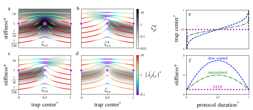
Figure 4: Geodesics and components of the friction matrix used to design two-dimensional linear-response protocols. Grayscale heatmap: components of the friction as a function of the (dimensionless) trap center^∗ $x^{\rm c}/{\Delta x_{\rm m}}$ and stiffness^∗ $kx_{\rm m}^{2}/E_{\rm B}$. Colored curves: geodesics of the friction for equal initial and final trap stiffness ($k_{\rm i}=k_{\rm f}$). Color heatmap: absolute product of control-parameter speeds $\dot{\lambda}_{j}=\mathrm{d}\lambda_{j}/\mathrm{d}t$. In the friction, the subscript ${\rm c}$ refers to the trap center and ${\rm s}$ to the stiffness components of the matrix. The positive and negative components of the off-diagonal entry $\zeta_{\rm c,s}$ are respectively denoted by $\zeta_{\rm c,s}^{+}\equiv{\rm max}(\zeta_{\rm c,s},0)$ (b) and $\zeta_{\rm c,s}^{-}\equiv{\rm max}(-\zeta_{\rm c,s},0)$ (c). The stars in (a-d) denote the STEP for initial and final stiffness $kx_{\rm m}^{2}/E_{\rm B}=1$. (e,f) STEP (purple dotted) as a function of protocol duration, with the corresponding slow (blue dashed) and interpolated protocols (green dot-dashed). An asterisk denotes a scaled (dimensionless) quantity, with the velocities scaled by the average speed $|\dot{\lambda}_{j}\dot{\lambda}_{\ell}|^{*}\equiv|\dot{\lambda}_{j}\dot{\lambda}_{\ell}|/(\overline{|\dot{\lambda}_{j}|}~{}\overline{|\dot{\lambda}_{\ell}|})$, friction as $\zeta_{j\ell}^{*}\equiv\zeta_{j\ell}\lambda_{j}\lambda_{\ell}/(\lambda_{j}^{*}\lambda_{\ell}^{*}\gamma x_{\rm m}^{2})$, and protocol duration as $t/\Delta t$. This figure is adapted from Fig. S1 of the supplemental material in Ref. Blaber and Sivak, 2022b.

Some general properties can be observed from Fig. 4: although the friction is positive semidefinite, the off-diagonal component can become negative; geodesics never have any discontinuities (following from the Riemannian geometry); geodesics tend to avoid or slow down in regions of high friction; and for driven barrier crossing the minimum-work protocol slows down and tightens the trap as it crosses the barrier. Slowing down and tightening the trap as the system crosses the barrier is consistent with the results derived within the strong-trap approximation (section IV.2); however, the designed slow-control protocol lacks the jumps at the start and end of the protocol.

Extensions to the slow-control approximation

The slow-driving approximation has been generalized and extended to transitions between nonequilibrium steady states Mandal and Jarzynski (2016); Zulkowski et al. (2013), discrete control Large and Sivak (2019), and stochastic control Large et al. (2018).

Previously throughout section V, we assumed that the system starts in equilibrium; however, this is not always the case in applications. Periodically driven machines such as ATP synthase are often driven for a sufficiently long time as to reach a nonequilibrium steady state, breaking the initial-equilibrium and near-equilibrium assumptions. Such systems may need to transition between steady states in order to increase or decrease their output in response to variable conditions (e.g., increasing/decreasing rate of ATP production). Although determining the correct definition of dissipation is more subtle for nonequilibrium steady states (see Refs. Oono and Paniconi, 1998; Hatano and Sasa, 2001; Speck and Seifert, 2005; Ge, 2009; Ge and Qian, 2010; Bertini et al., 2012, 2013, 2015 for detailed discussion), the slow-protocol approximation has been generalized to slow transitions between nonequilibrium steady states making use of a near-steady state approximation Mandal and Jarzynski (2016); Zulkowski et al. (2013). This approximation has an analogous form to the friction-tensor approximation and can be used to determine minimum-dissipation protocols for slow transitions between nonequilibrium steady states.

So far we have assumed that the protocol is continuous; however, many biological and chemical systems convert free energy stored in nonequilibrium chemical-potential differences into useful work through a series of reactions involving binding/unbinding or catalysis of small molecules. These chemical reactions typically occur on timescales much faster than the protein conformational rearrangements they couple to. Therefore, these changes are effectively instantaneous, leading to discrete control protocols. Building off of quasistatic results Nulton et al. (1985), it has been shown that the linear-response approximation can be applied to discretely driven systems to yield an approximation analogous to the friction tensor, which can be used to determine minimum-dissipation protocols Large and Sivak (2019).

The deterministic control considered in all other sections is a reasonable assumption for single-molecule experiments; however, autonomous systems such as ATP synthase in vivo are driven not by a deterministic controller, but by other stochastic systems. Towards a description of fully autonomous machines, several advances have been made extending the friction-tensor framework to stochastic control Large et al. (2018) and autonomous thermodynamic cycles Bryant and Machta (2020). A detailed discussion of protocol optimization for stochastic control, as well as relations to other bounds on dissipation Machta (2015) appears in Ref. Large et al., 2018.

Higher-order moments and corrections

For moderate-to-fast driving, the slow-control approximation is not sufficient to accurately determine the minimum-dissipation protocol. The slow-control approximation can be generalized to higher-order moments of the work distribution and to account for the next-order correction to the excess work.Blaber and Sivak (2020b) This is particularly useful for nonequilibrium free-energy estimation (section VI).

In Ref. Blaber and Sivak, 2020b, the higher-order corrections are derived for the first moment

$$\langle W_{\rm ex}\rangle_{\Lambda} \approx\int_{0}^{\Delta t}\mathrm{d}t~{}\left\{\zeta_{j\ell}[\boldsymbol{\lambda}(t)]+\frac{1}{4}\zeta^{(2)}_{j\ell m}[\boldsymbol{\lambda}(t)]\dot{\lambda}_{m}(t)\right\}\dot{\lambda}_{j}(t)\dot{\lambda}_{\ell}(t)\ ,$$ (46)

second moment

$$\langle W_{\rm ex}^{2}\rangle_{\Lambda} \approx\frac{2}{\beta}\int_{0}^{\Delta t}\mathrm{d}t~{}\left\{\zeta_{j\ell}[\boldsymbol{\lambda}(t)]+\frac{3}{4}\zeta^{(2)}_{j\ell m}[\boldsymbol{\lambda}(t)]\dot{\lambda}_{m}(t)\right\}\dot{\lambda}_{j}(t)\dot{\lambda}_{\ell}(t)\ .$$ (47)

and $n^{\rm th}$ moment

$$\beta^{n-1}\langle W_{\rm ex}^{n}\rangle_{\Lambda}\approx\int_{0}^{\Delta t}\mathrm{d}t~{}\left\{n\mathcal{C}_{\nu_{1}\cdots\nu_{n}}^{(n-1)}[\boldsymbol{\lambda}(t),t]+\frac{n+1}{2}\mathcal{C}_{\nu_{1}\cdots\nu_{n+1}}^{(n)}[\boldsymbol{\lambda}(t),t]\dot{\lambda}_{\nu_{n+1}}(t)\right\}\prod_{j=1}^{n}\dot{\lambda}_{\nu_{j}}(t)\ .$$ (48)

We have defined the rank-three tensor

$$\zeta_{j\ell m}^{(2)}[\boldsymbol{\lambda}(t)]\equiv-\beta^{2}\int_{0}^{\infty}\mathrm{d}t^{\prime\prime}\int_{0}^{\infty}\mathrm{d}t^{\prime\prime\prime}\left\langle\delta f_{j}(0)\delta f_{\ell}(t^{\prime\prime})\delta f_{m}(t^{\prime\prime\prime})\right\rangle_{\boldsymbol{\lambda}(t)}\ ,$$ (49)

and the integral $n$-time covariance functions

$$\mathcal{C}_{\nu_{1}\cdots\nu_{n}}^{(n-1)} [\boldsymbol{\lambda}(t),t]\equiv(-\beta)^{n}\prod_{j=2}^{n}\int_{0}^{t}\mathrm{d}t_{j}\left\langle\prod_{\ell=2}^{n}\delta f_{\nu_{1}}(0)\delta f_{\nu_{\ell}}(t_{\ell})\right\rangle_{\boldsymbol{\lambda}(t)}\ .$$ (50)

The rank-three tensor [Eq. (49)] is referred to as the supra-Stokes’ tensor and is indexed by superscript (2), as it corresponds to the next-order correction to dissipation beyond the Stokes’ friction (46). The higher-order moments of the excess work are higher order in control-parameter velocity and are therefore smaller for slow protocols.

The most notable application of this approximation is to free-energy estimation (section VI), where the supra-Stokes’ tensor determines the leading-order contribution to the bias of bidirectional estimators and can be used to design protocols that minimize bias Blaber and Sivak (2020b).

V.4 Interpolated protocols

Given theory describing minimum-dissipation control in both the slow and fast limits, a simple interpolation scheme has been developed to design protocols that reduce dissipation at all driving speeds Blaber et al. (2021); Blaber and Sivak (2022b). The interpolated protocol has an initial jump $(\boldsymbol{\lambda}^{\rm STEP}-\boldsymbol{\lambda}_{\rm i})/(1+\Delta t/\tau)$ and a final jump $(\boldsymbol{\lambda}_{\rm f}-\boldsymbol{\lambda}^{\rm STEP})/(1+\Delta t/\tau)$, and follows the slow-control path between them,

$$\boldsymbol{\lambda}^{\rm interp}(t)=\frac{1}{1+\frac{\Delta t}{\tau}}\boldsymbol{\lambda}^{\rm STEP}+\left(1-\frac{1}{1+\frac{\Delta t}{\tau}}\right)\boldsymbol{\lambda}^{\rm slow}(t)\ ,$$ (51)

with $\tau$ the crossover duration and $\boldsymbol{\lambda}^{\rm slow}(t)$ the solution to (45). This guarantees that the protocol approaches the minimum-dissipation protocol in both the fast and slow limits.

VI Free-Energy Estimation

Computational and experimental measurements of free-energy differences are essential to the determination of stable equilibrium phases of matter, relative reaction rates, and binding affinities of chemical species,Gapsys et al. (2015) and the identification and design of novel protein-binding ligands for drug discovery.Schindler et al. (2020); Kuhn et al. (2017); Ciordia et al. (2016); Wang et al. (2015) Current methods for determining free-energy differences rely on costly experimentation, which can be reduced through screening with efficient computational techniques.Schindler et al. (2020); Aldeghi et al. (2018); Kuhn et al. (2017); Ciordia et al. (2016); Wang et al. (2015); Gapsys et al. (2015); Chodera et al. (2011); Pohorille et al. (2010) It has been shown that the precision and accuracy of standard free-energy estimators are reduced when estimated from a protocol inducing large dissipation,Gore et al. (2003); Shenfeld et al. (2009); Blaber and Sivak (2020b) and that thermodynamic geometry can be applied to improve free-energy estimates.Shenfeld et al. (2009); Minh (2020); Pham and Shirts (2011, 2012); Park and Im (2014); Blaber and Sivak (2020b)

Free-energy differences are often estimated by measuring the work incurred during a parametric control protocol that drives the system between control-parameter endpoints corresponding to target states. Unidirectional estimators determine the free-energy difference from the work done by a forward protocol driving from initial to final control-parameter values, while bidirectional estimators additionally use reverse protocols that drive from final to initial control-parameter values. The simplest estimator is the mean-work estimator,Gore et al. (2003) which estimates the free-energy difference by the average work and for any non-quasistatic (finite-speed) protocol yields a biased estimate. For an unbiased estimate, the Jarzynski estimator (derived from the Jarzynski equality Jarzynski (1997)) estimates the free-energy difference from the exponentially averaged work. The mean-work and Jarzynski estimators can be used as either uni- or bidirectional estimators; however, if bidirectional data is available the maximum log-likelihood estimator is Bennett’s acceptance ratio.Bennett (1976) For a large number of samples, Bennett’s acceptance ratio yields the minimum variance of any unbiased estimator.Shirts et al. (2003); Maragakis et al. (2006)

Near equilibrium, Taylor expanding all of these estimators for small excess work (small dissipation) gives the mean-work estimator. Blaber and Sivak (2020b) For an equal number of samples in the forward and reverse directions, near equilibrium the variance of any of these estimators is Blaber and Sivak (2020b)

$$\left\langle\left(\delta\widehat{\Delta F}\right)^{2}\right\rangle \approx\frac{\langle W_{\rm ex}^{2}\rangle_{\Lambda}+\langle W_{\rm ex}^{2}\rangle_{{\Lambda^{\dagger}}}}{2N}$$ (52a)

$$\approx\frac{\langle W_{\rm ex}\rangle_{\Lambda}+\langle W_{\rm ex}\rangle_{{\Lambda^{\dagger}}}}{N}\ ,$$ (52b)

where the second line follows from the fluctuation-dissipation relation for the work distribution. Gore et al. (2003); Blaber and Sivak (2020b) The bias is given by the asymmetry between forward $\Lambda$ and reverse $\Lambda^{\dagger}$ dissipation, generated from skewed work fluctuations:

$$\left\langle\delta\widehat{\Delta F}\right\rangle \approx\frac{\langle W_{\rm ex}\rangle_{\Lambda}-\langle W_{\rm ex}\rangle_{\Lambda^{\dagger}}}{2N}\ .$$ (53)

Equations (52a) and (53) not only hold near equilibrium but also when only a single sample is taken in the forward and reverse directions, since then the average of a function is equal to the function of the average (e.g., $\langle e^{x}\rangle=e^{\langle x\rangle}$).

For a slow protocol the variance is approximated by

$$\left\langle\left(\delta\widehat{\Delta F}\right)^{2}\right\rangle\approx\frac{2}{\beta N}\int_{0}^{\Delta t}\mathrm{d}t\,\zeta_{j\ell}[\boldsymbol{\lambda}(t)]\dot{\lambda}_{j}(t)\dot{\lambda}_{\ell}(t)\ ,$$ (54)

Thus the protocol designed to reduce the variance follows geodesics of $\zeta_{j\ell}$, and for one-dimensional control proceeds at velocity $\dot{\lambda}\propto\left(\zeta\right)^{-1/2}$. This, or the related force-variance metric Shenfeld et al. (2009), has been used to improve the precision of calculated binding potentials of mean force Minh (2020); Pham and Shirts (2011, 2012); Park and Im (2014).

Unlike the variance, the protocol that maximizes the accuracy (minimizes bias) is different for unidirectional and bidirectional estimators. For unidirectional Jarzynski and mean-work estimators, near equilibrium the minimum-bias protocol is simply the minimum-dissipation protocol (protocol that minimizes (46)) and therefore to leading order is optimized by the same protocol that minimizes (54). For a slow protocol, the bias from Bennett’s acceptance ratio can be approximated as

$$\left\langle\delta\widehat{\Delta F}\right\rangle \approx\frac{1}{4N}\int_{0}^{\Delta t}\mathrm{d}t\,\zeta^{(2)}_{j\ell m}[\boldsymbol{\lambda}(t)]\,\dot{\lambda}_{j}(t)\dot{\lambda}_{\ell}(t)\dot{\lambda}_{m}(t)\ ,$$ (55)

where the second line follows from (46). The protocol designed to reduce the (magnitude of) bias thus follows geodesics of the cubic Finsler metric $\zeta^{(2)}_{j\ell m}$, simplifying for one-dimensional control to $\dot{\lambda}\propto\left(\zeta^{(2)}\right)^{-1/3}$.

VII Comparison between control strategies

In this section we compare naive and designed protocols based on the methods described in the previous sections: interpolated protocols combining STEP and slow-protocol approximations (section V.4), strong-trap approximation (section IV.2), and full control (section IV.1). We again turn to the example model system of driven barrier crossing to assess similarities, differences, and performance of the designed protocols. The naive protocol serves as a baseline which the designed protocols should outperform, and full control as a bound on what parametric control could possibly achieve.

Fig. 5 shows the naive and designed protocols for intermediate driving speed, intermediate trap stiffness, and for fixed final control parameters. Every designed protocol has discontinuous jumps at the start and end of the protocol, and slows down and tightens the trap as it crosses the barrier. The behavior of the designed protocols can be understood in terms of the full-control solution. In one dimension the minimum-dissipation protocol linearly drives the quantiles of the probability distribution between the initial and final distributions. In the naive protocol, since it has constant stiffness, the probability distribution spreads out as it crosses the barrier due to the negative curvature of the energy landscape at the barrier. To compensate for this, the designed protocols tighten as they cross the barrier; additionally, to compensate for the changes in the gradient of the energy landscape, the designed protocols slow down as they cross the barrier.

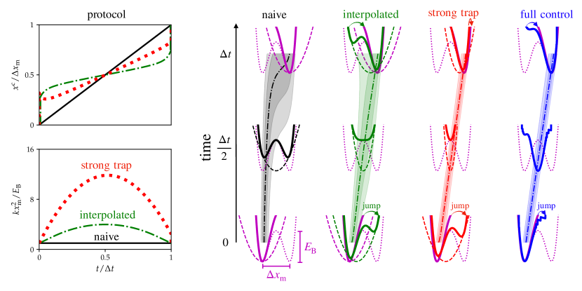
Figure 5: Time-dependent protocols for driven barrier crossing at intermediate protocol duration. Naive (black), interpolated (green), strong-trap (red), and full-control (blue) protocols. Snapshots of the total (solid), static hairpin (dotted), and time-dependent trap (dashed) potential are shown for $t=0$, $\Delta t/2$, and $\Delta t$. The hairpin, initial, and final potentials are the same across protocols (purple). Dash-dotted curves: median positions during corresponding protocol. Shading: 9%, 25%, 75%, and 91% quantiles, which are approximately evenly spaced for a Gaussian distribution. Barrier height is $E_{\rm B}=4\beta^{-1}$, initial and final trap stiffnesses are $k_{\rm i}=k_{\rm f}=4\beta^{-1}/x_{\rm m}^{2}$, and protocol duration is $\tau_{\rm D}$ for diffusion time $\tau_{\rm D}=\Delta x_{\rm m}^{2}/(2D)$.

Fig. 6 shows the excess work of the designed protocols compared to the naive protocol. For long duration (slow protocol) all of the designed protocols significantly outperform the naive, with the difference between the minimum dissipation possible from full control indistinguishable from the dissipation from the interpolated protocol in this limit. While the approximations made in the interpolated protocol become exact in the long-duration limit, the same is not true for the strong-trap approximation. As a result, the strong-control protocol has slightly higher dissipation in the long-duration limit, but would achieve the minimal dissipation in the limit of high trap stiffness. Furthermore, for intermediate protocol duration ($\Delta t\sim\tau_{\rm D}$), the strong control performs the best of the approximations since the approximation does not explicitly depend on the protocol duration. For short duration (fast protocols), all the designed protocols perform similarly well.

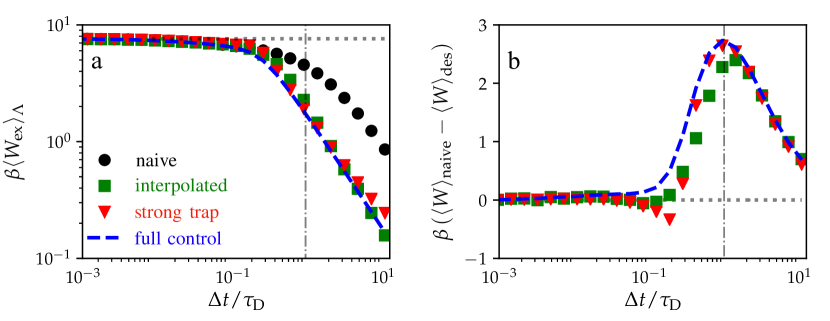
Figure 6: Performance of the naive (black circles), interpolated (green squares), strong-trap (red triangles), and full-control (blue dashed) protocols. (a) Excess work $\langle W_{\rm ex}\rangle_{\boldsymbol{\Lambda}}$ and (b) work difference $\langle W\rangle_{\rm naive}-\langle W\rangle_{\rm des}$ between designed and naive protocols, all as functions of protocol duration $\Delta t/\tau_{\rm D}$ scaled by diffusion time $\tau_{\rm D}$. Error bars representing bootstrap-resampled 95% confidence intervals are smaller than the markers.

In summary, the designed protocols perform similarly well, so it seems reasonable to choose the control strategy which is simplest to determine, provided the approximations/assumptions required are satisfied. Since the strong-trap approximation has explicit solutions for the designed protocol, it will generally be the simplest to determine; however, it is not as widely applicable as the interpolated protocols.

VIII Perspective and outlook

We have reviewed optimal control in stochastic thermodynamics, from full control (section IV) to parametric control (section V). General methods are known for determining minimum-dissipation protocols for parametric control ranging from strong (section IV.2) to weak (section V.2) and fast (section V.1) to slow (section V.3). These approximations fill out the four limits of parametric control (Fig. 2) and can be combined to design protocols that reduce dissipation at any driving speed (section V.4). These designed protocols reproduce key features determined by exact solutions for Gaussian distributions and quadratic trapping potentials, such as control-parameter jumps at the start and end of the protocol (section V.1) and linear driving of the distribution quantiles between specified endpoints (section IV.1).

For the model system of driven barrier crossing (section II), we compare the interpolated, strong-control, and full-control solutions (section VII). The designed protocols significantly outperform the naive (linear) protocol. Strong control has explicit solutions for the minimum-dissipation protocol, making it the simplest approximation to use; however, it is only applicable to overdamped dynamics with strong trapping potentials.

Figure 2 shows the limits in which we have solutions for the minimum-dissipation protocol for parametric control. The linear-response and slow-driving approximations have been applied to several different types of systems and control (section V.3). A promising area of future study would be to explore if extensions and generalizations can be made to strong and fast control. Indeed, it has recently been shown that the fast-protocol approximation can be extended to quantum systems, classical Hamiltonian dynamics, and optimization of the variance of the work distribution.Rolandi et al. (2022)

Another extension to consider is to allow for position-dependent diffusivity, which generically arises when a high-dimensional system is represented in a lower-dimensional space.Best and Hummer (2010) For example, DNA hairpin experiments and molecular dynamics simulations take place in three spatial dimensions but are often represented as one-dimensional diffusive processes.Hummer (2005); Neupane et al. (2016, 2017) This requires averaging out the behavior in the other two dimensions, and any inhomogeneity in these dimensions will result in position-dependent effective diffusivity in the one-dimensional representation. Measured diffusivities in molecular dynamics simulations often vary with position Hummer (2005), and although accurate measurements remain a technical challenge, some hairpin experiments report a position-dependent diffusivity.Foster et al. (2018) Position-dependent diffusivity can alter the kinetic transition state of protein folding Chahine et al. (2007), which will impact the design of minimum-dissipation protocols. Therefore, position-dependent diffusivity may be an important consideration in some applications. The minimum-dissipation protocol under full control in inhomogeneous environments (e.g., position-dependent diffusivity) has been treated in detail in Ref. 157.

An important aspect of designing protocols to minimize dissipation in both experiments and theory is the choice of control parameters and number of control parameters. For the model system of driven barrier crossing, it has been shown that designed protocols with control over both trap center and stiffness (two-parameter control) significantly reduces dissipation compared to designed protocols that can only adjust the trap center (single-parameter control). Blaber and Sivak (2022b) However, adding even more control parameters does not significantly reduce dissipation any further, because this system is well approximated as a one-dimensional Gaussian, for which the full-control solution only requires two parameters to adjust the mean and variance (section IV.1). Although this phenomenon is well explained for one-dimensional overdamped systems, considerably less is known more generally. For example, Ref. Louwerse and Sivak, 2022 compared one-, two-, and four-parameter control of the Ising model and found significant qualitative and quantitative differences between the designed protocols. Since the full-control solution for this system is not yet known, we cannot explain this phenomenon the same way we did for driven barrier crossings. Beyond simply the number of control parameters, it remains an open question as to which control parameters are the most important when designing protocols to minimize dissipation. The choice of control parameters and number of control parameters will be important for experimental and computational applications, such as free-energy estimation.

Leveraging optimal-transport theory appears to be a promising approach towards a deeper understanding of optimal control in stochastic thermodynamics. Full-control solutions based on optimal-transport theory were initially only applicable to continuous classical systems with overdamped dynamics Aurell et al. (2011); Nakazato and Ito (2021); however, recent studies have begun to expand their range of applicability to discrete-state and quantum systems Dechant (2022); Dechant et al. (2022); Yoshimura et al. (2022); Zhong and DeWeese (2022); Van Vu and Saito (2023a); Van Vu and Saito (2023b).

The full-control solutions give an idealized view of optimal control and will always outperform parametric control, but can be used as the ideal solution that parametric control can strive towards and draw insight from. For example, linearly driving the quantiles between the initial and final endpoints is the minimum-dissipation protocol for a one-dimensional system under full control; this is reasonably well reproduced by parametric control of driven barrier crossing (section VII). Furthermore, it has recently been shown that optimal-transport theory can be leveraged to design minimum-dissipation protocols under parametric control Zhong and DeWeese (2022), which is a promising new technique for determining exact minimum-dissipation protocols at any driving speed or strength of driving.

In this review we focused on protocols which reduce the average work or entropy production; however, higher-order moments (e.g., variance or skewness), or individual trajectory optimization Proesmans (2022) may also be of interest for strongly fluctuating systems. Ref. Solon and Horowitz, 2018 compared for a breathing harmonic trap the protocols that minimize work variance with those that minimize average work, finding that minimum-average-work and minimum-work-variance protocols qualitatively differ for intermediate-to-fast driving speeds. In contrast, for slow near-equilibrium control, the same protocols minimize average work and work variance (section V.3), so a more complete description of minimum-variance protocols far from equilibrium is desirable.

This review has focused on systems driven by external control parameters, which is adequate for describing the experimental systems discussed in section II; however, this does not accurately describe autonomous machines. For example, ATP synthase in vivo is driven by a proton gradient across the mitochondrial membrane which drives the coupled ${\rm F}_{\rm o}$ and ${\rm F}_{1}$ components. In this system, coupling between the components means that none of the components can be treated as external, and thus it is not obvious how the present discussion of optimal control applies to such autonomous machines. Some first steps towards the description of autonomous molecular machines is discussed in section V.3; however, more work is required towards a full description of efficient autonomous machines.Ehrich and Sivak (2023)

The majority of the studies on optimal control in stochastic thermodynamics have focused on theoretical understanding and simple toy models. As we have shown in this review, there is a deep understanding of minimum-dissipation protocols at both slow and fast driving speed and both weak and strong driving strength (Fig. 2). It would be interesting to see how these results apply to real physical systems and if they are able to achieve the promising results predicted by theory. The two most straightforward applications are to relatively simple experimental model systems (section II) in an analogous fashion to Ref. Tafoya et al., 2019, and to free-energy estimation as discussed in section VI, in a similar fashion to Refs. Minh, 2020; Pham and Shirts, 2011, 2012; Park and Im, 2014.

References

- Andresen et al. (1977) B. Andresen, R. S. Berry, A. Nitzan, and P. Salamon, Phys. Rev. A 15, 2086 (1977).
- Salamon et al. (1977) P. Salamon, B. Andresen, and R. S. Berry, Phys. Rev. A 15, 2094 (1977).
- Andresen (2011) B. Andresen, Angew. Chem. Int. Ed. 50, 2690 (2011).
- Band et al. (1982) Y. B. Band, O. Kafri, and P. Salamon, J. Appl. Phys. 53, 8 (1982).
- Weinhold (1975) F. Weinhold, J. Chem. Phys. 63, 2479 (1975).
- Ruppeiner (1979) G. Ruppeiner, Phys. Rev. A 20, 1608 (1979).
- Crooks (2007) G. E. Crooks, Phys. Rev. Lett. 99, 100602 (2007).
- Salamon and Berry (1983) P. Salamon and R. S. Berry, Phys. Rev. Lett. 51, 1127 (1983).
- Ashkin (1970) A. Ashkin, Phys. Rev. Lett. 24, 156 (1970).
- Bustamante et al. (2021) C. J. Bustamante, Y. R. Chemla, S. Liu, and M. D. Wang, Nat. Rev. Methods Primers 1, 1 (2021).
- Polimeno et al. (2018) P. Polimeno, A. Magazzu, M. A. Iati, F. Patti, R. Saija, C. D. E. Boschi, M. G. Donato, P. G. Gucciardi, P. H. Jones, G. Volpe, et al., J. Quant. Spectrosc. Radiat. Transf. 218, 131 (2018).
- Moffitt et al. (2008) J. R. Moffitt, Y. R. Chemla, S. B. Smith, and C. Bustamante, Annu. Rev. Biochem. 77, 205 (2008).
- Liphardt et al. (2002) J. Liphardt, S. Dumont, S. B. Smith, I. Tinoco, and C. Bustamante, Science 296, 1832 (2002).
- Collin et al. (2005) D. Collin, F. Ritort, C. Jarzynski, S. B. Smith, I. Tinoco, and C. Bustamante, Nature 437, 231 (2005).
- Bustamante et al. (2000) C. Bustamante, S. B. Smith, J. Liphardt, and D. Smith, Curr. Opin. Struct. Biol. 10, 279 (2000).
- Bustamante et al. (2003) C. Bustamante, Z. Bryant, and S. B. Smith, Nature 421, 423 (2003).
- Woodside et al. (2006) M. T. Woodside, W. M. Behnke-Parks, K. Larizadeh, K. Travers, D. Herschlag, and S. M. Block, Proc. Natl. Acad. Sci. U.S.A 103, 6190 (2006).
- Neupane et al. (2017) K. Neupane, F. Wang, and M. T. Woodside, Proc. Natl. Acad. Sci. U.S.A 114, 1329 (2017).
- Unksov et al. (2022) I. N. Unksov, C. S. Korosec, P. Surendiran, D. Verardo, R. Lyttleton, N. R. Forde, and H. Linke, ACS nanoscience Au 2, 140 (2022).
- Toyabe et al. (2011) S. Toyabe, T. Watanabe-Nakayama, T. Okamoto, S. Kudo, and E. Muneyuki, Proc. Natl. Acad. Sci. U.S.A 108, 17951 (2011).
- Toyabe et al. (2012) S. Toyabe, H. Ueno, and E. Muneyuki, Europhys. Lett. 97, 40004 (2012).
- Kawaguchi et al. (2014) K. Kawaguchi, S.-i. Sasa, and T. Sagawa, Biophys. J. 106, 2450 (2014).
- Svoboda et al. (1993) K. Svoboda, C. F. Schmidt, B. J. Schnapp, and S. M. Block, Nature 365, 721 (1993).
- Svoboda and Block (1994) K. Svoboda and S. M. Block, Cell 77, 773 (1994).
- Kojima et al. (1997) H. Kojima, E. Muto, H. Higuchi, and T. Yanagida, Biophys. J. 73, 2012 (1997).
- Hunt et al. (1994) A. J. Hunt, F. Gittes, and J. Howard, Biophys. J. 67, 766 (1994).
- Greenberg et al. (2016) M. Greenberg, G. Arpağ, E. Tüzel, and E. Ostap, Biophys. J. 110, 2568 (2016).
- Laakso et al. (2008) J. M. Laakso, J. H. Lewis, H. Shuman, and E. M. Ostap, Science 321, 133 (2008).
- Norstrom et al. (2010) M. F. Norstrom, P. A. Smithback, and R. S. Rock, J. Biol. Chem. 285, 26326 (2010).
- Nagy et al. (2013) A. Nagy, Y. Takagi, N. Billington, S. A. Sun, D. K. Hong, E. Homsher, A. Wang, and J. R. Sellers, J. Biol. Chem. 288, 709 (2013).
- Seifert (2012) U. Seifert, Rep. Prog. Phys. 75, 126001 (2012).
- Jarzynski (2011) C. Jarzynski, Annu. Rev. Condens. Matter Phys. 2, 329 (2011).
- Brown and Sivak (2017) A. I. Brown and D. A. Sivak, Physics in Canada 73 (2017).
- Brown and Sivak (2019) A. I. Brown and D. A. Sivak, Chem. Rev. 120, 434 (2019).
- Schmiedl and Seifert (2007) T. Schmiedl and U. Seifert, Phys. Rev. Lett. 98, 108301 (2007).
- Abiuso et al. (2022) P. Abiuso, V. Holubec, J. Anders, Z. Ye, F. Cerisola, and M. Perarnau-Llobet, J. Phys. Commun. 6, 063001 (2022).
- Blaber and Sivak (2022a) S. Blaber and D. A. Sivak, Phys. Rev. E 106, L022103 (2022a).
- Gomez-Marin et al. (2008) A. Gomez-Marin, T. Schmiedl, and U. Seifert, J. Chem. Phys. 129, 024114 (2008).
- Then and Engel (2008) H. Then and A. Engel, Phys. Rev. E 77, 041105 (2008).
- Esposito et al. (2010a) M. Esposito, R. Kawai, K. Lindenberg, and C. Van den Broeck, Europhys. Lett. 89, 20003 (2010a).
- Blaber et al. (2021) S. Blaber, M. D. Louwerse, and D. A. Sivak, Phys. Rev. E 104, L022101 (2021).
- Villani (2009) C. Villani, Optimal transport: old and new, vol. 338 (Springer, 2009).
- Santambrogio (2015) F. Santambrogio, Optimal transport for applied mathematicians, vol. 55 (Springer, 2015).
- Aurell et al. (2011) E. Aurell, C. Mejía-Monasterio, and P. Muratore-Ginanneschi, Phys. Rev. Lett. 106, 250601 (2011).
- Zhang (2019) Y. Zhang, Europhys. Lett. 128, 30002 (2019).
- Nakazato and Ito (2021) M. Nakazato and S. Ito, Phys. Rev. Res. 3, 043093 (2021).
- Dechant (2022) A. Dechant, J. Phys. A Math. Theor. 55, 094001 (2022).
- Miangolarra et al. (2022) O. M. Miangolarra, A. Taghvaei, Y. Chen, and T. T. Georgiou, IEEE Contr. Syst. Lett. 6, 3409 (2022).
- Benamou and Brenier (2000) J.-D. Benamou and Y. Brenier, Numerische Mathematik 84, 375 (2000).
- Proesmans et al. (2020a) K. Proesmans, J. Ehrich, and J. Bechhoefer, Phys. Rev. Lett. 125, 100602 (2020a).
- Proesmans et al. (2020b) K. Proesmans, J. Ehrich, and J. Bechhoefer, Phys. Rev. E 102, 032105 (2020b).
- Dechant et al. (2022) A. Dechant, S.-i. Sasa, and S. Ito, Phys. Rev. Res. 4, L012034 (2022).
- Yoshimura et al. (2022) K. Yoshimura, A. Kolchinsky, A. Dechant, and S. Ito, arXiv preprint arXiv:2205.15227 (2022).
- Zhong and DeWeese (2022) A. Zhong and M. R. DeWeese, Phys. Rev. E 106, 044135 (2022).
- Van Vu and Saito (2023a) T. Van Vu and K. Saito, Phys. Rev. X 13, 011013 (2023a).
- Van Vu and Saito (2023b) T. Van Vu and K. Saito, Phys. Rev. Lett. 130, 010402 (2023b).
- Gingrich et al. (2016) T. R. Gingrich, G. M. Rotskoff, G. E. Crooks, and P. L. Geissler, Proc. Natl. Acad. Sci. U.S.A. 113, 10263 (2016).
- Engel et al. (2022) M. C. Engel, J. A. Smith, and M. P. Brenner, arXiv preprint arXiv:2201.00098 (2022).
- Bonança and Deffner (2018) M. V. Bonança and S. Deffner, Phys. Rev. E 98, 042103 (2018).
- Kamizaki et al. (2022) L. P. Kamizaki, M. V. Bonança, and S. R. Muniz, Phys. Rev. E 106, 064123 (2022).
- Sivak and Crooks (2016) D. A. Sivak and G. E. Crooks, Phys. Rev. E 94, 052106 (2016).
- Blaber and Sivak (2020a) S. Blaber and D. A. Sivak, Phys. Rev. E 101, 022118 (2020a).
- Deffner and Bonança (2020) S. Deffner and M. V. Bonança, Europhys. Lett. 131, 20001 (2020).
- Zulkowski et al. (2012) P. R. Zulkowski, D. A. Sivak, G. E. Crooks, and M. R. DeWeese, Phys. Rev. E 86, 041148 (2012).
- Bonança and Deffner (2014) M. V. Bonança and S. Deffner, J. Chem. Phys. 140, 244119 (2014).
- Zulkowski and DeWeese (2015a) P. R. Zulkowski and M. R. DeWeese, Phys. Rev. E 92, 032117 (2015a).
- Zulkowski and DeWeese (2015b) P. R. Zulkowski and M. R. DeWeese, Phys. Rev. E 92, 032113 (2015b).
- Large and Sivak (2019) S. J. Large and D. A. Sivak, J. Stat. Mech.: Theory Exp. 2019, 083212 (2019).
- Lucero et al. (2019) J. N. Lucero, A. Mehdizadeh, and D. A. Sivak, Phys. Rev. E 99, 012119 (2019).
- Rotskoff and Crooks (2015) G. M. Rotskoff and G. E. Crooks, Phys. Rev. E 92, 060102 (2015).
- Rotskoff et al. (2017) G. M. Rotskoff, G. E. Crooks, and E. Vanden-Eijnden, Phys. Rev. E 95, 012148 (2017).
- Louwerse and Sivak (2022) M. D. Louwerse and D. A. Sivak, J. Chem. Phys 156, 194108 (2022).
- Frim and DeWeese (2022a) A. G. Frim and M. R. DeWeese, Phys. Rev. E 105, L052103 (2022a).
- Frim and DeWeese (2022b) A. G. Frim and M. R. DeWeese, Phys. Rev. Lett. 128, 230601 (2022b).
- Tafoya et al. (2019) S. Tafoya, S. J. Large, S. Liu, C. Bustamante, and D. A. Sivak, Proc. Natl. Acad. Sci. U.S.A 116, 5920 (2019).
- Blaber and Sivak (2020b) S. Blaber and D. A. Sivak, J. Chem. Phys. 153, 244119 (2020b).
- Blaber and Sivak (2022b) S. Blaber and D. A. Sivak, Europhys. Lett. 139, 17001 (2022b).
- Holubec and Ryabov (2021) V. Holubec and A. Ryabov, J. Phys. A Math. Theor. 55, 013001 (2021).
- Ma et al. (2018a) Y.-H. Ma, D. Xu, H. Dong, and C.-P. Sun, Phys. Rev. E 98, 022133 (2018a).
- Zhang (2020) Y. Zhang, J. Stat. Phys. 178, 1336 (2020).
- Abiuso and Perarnau-Llobet (2020) P. Abiuso and M. Perarnau-Llobet, Phys. Rev. Lett. 124, 110606 (2020).
- Chen (2022) J.-F. Chen, Phys. Rev. E 106, 054108 (2022).
- Curzon and Ahlborn (1975) F. L. Curzon and B. Ahlborn, Am. J. Phys. 43, 22 (1975).
- Van den Broeck (2005) C. Van den Broeck, Phys. Rev. Lett. 95, 190602 (2005).
- Schmiedl and Seifert (2008) T. Schmiedl and U. Seifert, Europhys. Lett. 83, 30005 (2008).
- Esposito et al. (2009) M. Esposito, K. Lindenberg, and C. Van den Broeck, Phys. Rev. Lett. 102, 130602 (2009).
- Esposito et al. (2010b) M. Esposito, R. Kawai, K. Lindenberg, and C. Van den Broeck, Phys. Rev. Lett. 105, 150603 (2010b).
- Brandner et al. (2015) K. Brandner, K. Saito, and U. Seifert, Phys. Rev. X. 5, 031019 (2015).
- Proesmans et al. (2016) K. Proesmans, B. Cleuren, and C. Van den Broeck, Phys. Rev. Lett. 116, 220601 (2016).
- Shiraishi et al. (2016) N. Shiraishi, K. Saito, and H. Tasaki, Phys. Rev. Lett. 117, 190601 (2016).
- Ma et al. (2018b) Y.-H. Ma, D. Xu, H. Dong, and C.-P. Sun, Phys. Rev. E 98, 042112 (2018b).
- Ma et al. (2020) Y.-H. Ma, R.-X. Zhai, J. Chen, C. Sun, and H. Dong, Phys. Rev. Lett. 125, 210601 (2020).
- Miller and Mehboudi (2020) H. J. Miller and M. Mehboudi, Phys. Rev. Lett. 125, 260602 (2020).
- Brandner and Saito (2020) K. Brandner and K. Saito, Phys. Rev. Lett. 124, 040602 (2020).
- Miangolarra et al. (2021) O. M. Miangolarra, R. Fu, A. Taghvaei, Y. Chen, and T. T. Georgiou, Phys. Rev. E 103, 062103 (2021).
- Watanabe and Minami (2022) G. Watanabe and Y. Minami, Phys. Rev. Res. 4, L012008 (2022).
- Acconcia et al. (2015) T. V. Acconcia, M. V. Bonança, and S. Deffner, Phys. Rev. E 92, 042148 (2015).
- Scandi and Perarnau-Llobet (2019) M. Scandi and M. Perarnau-Llobet, Quantum 3, 197 (2019).
- Takahashi (2017) K. Takahashi, New J. Phys. 19, 115007 (2017).
- Guéry-Odelin et al. (2019) D. Guéry-Odelin, A. Ruschhaupt, A. Kiely, E. Torrontegui, S. Martínez-Garaot, and J. G. Muga, Rev. Mod. Phys 91, 045001 (2019).
- Guéry-Odelin et al. (2022) D. Guéry-Odelin, C. Jarzynski, C. A. Plata, A. Prados, and E. Trizac, Rep. Prog. Phys. (2022).
- Kumar and Bechhoefer (2018) A. Kumar and J. Bechhoefer, Appl. Phys. Lett. 113, 183702 (2018).
- Kumar and Bechhoefer (2019) A. Kumar and J. Bechhoefer, Physics in Canada 75 (2019).
- Gavrilov and Bechhoefer (2017) M. Gavrilov and J. Bechhoefer, Philos. Transact. A Math. Phys. Eng. Sci. 375, 20160217 (2017).
- Jun et al. (2014) Y. Jun, M. Gavrilov, and J. Bechhoefer, Phys. Rev. Lett. 113, 190601 (2014).
- Gavrilov and Bechhoefer (2016) M. Gavrilov and J. Bechhoefer, Phys. Rev. Lett. 117, 200601 (2016).
- Neupane et al. (2015) K. Neupane, A. P. Manuel, J. Lambert, and M. T. Woodside, J. Phys. Chem. Lett 6, 1005 (2015).
- Hong et al. (2016) J. Hong, B. Lambson, S. Dhuey, and J. Bokor, Sci. Adv. 2, e1501492 (2016).
- Gupta et al. (2022) D. Gupta, S. J. Large, S. Toyabe, and D. A. Sivak, J. Phys. Chem. Lett. 13, 11844 (2022).
- Park et al. (2003) S. Park, F. Khalili-Araghi, E. Tajkhorshid, and K. Schulten, J. Chem. Phys. 119, 3559 (2003).
- Park and Schulten (2004) S. Park and K. Schulten, J. Chem. Phys. 120, 5946 (2004).
- Dellago and Hummer (2014) C. Dellago and G. Hummer, Entropy 16, 41 (2014).
- Ito (2023) S. Ito, Info. Geo. pp. 1–42 (2023).
- Abreu and Seifert (2011) D. Abreu and U. Seifert, Europhys. Lett. 94, 10001 (2011).
- Olkin and Pukelsheim (1982) I. Olkin and F. Pukelsheim, Linear Algebr. Appl. 48, 257 (1982).
- Dechant and Sakurai (2019) A. Dechant and Y. Sakurai, arXiv preprint arXiv:1912.08405 (2019).
- Wang and Oster (2002) H. Wang and G. Oster, Europhys. Lett. 57, 134 (2002).
- Sivak and Crooks (2012) D. A. Sivak and G. E. Crooks, Phys. Rev. Lett. 108, 190602 (2012).
- Mandal and Jarzynski (2016) D. Mandal and C. Jarzynski, J. Stat. Mech. Theory Exp. 2016, 063204 (2016).
- Zulkowski et al. (2013) P. R. Zulkowski, D. A. Sivak, and M. R. DeWeese, PloS one 8, e82754 (2013).
- Large et al. (2018) S. J. Large, R. Chetrite, and D. A. Sivak, Europhys. Lett. 124, 20001 (2018).
- Oono and Paniconi (1998) Y. Oono and M. Paniconi, Progress of Theoretical Physics Supplement 130, 29 (1998).
- Hatano and Sasa (2001) T. Hatano and S.-i. Sasa, Phys. Rev. Lett. 86, 3463 (2001).
- Speck and Seifert (2005) T. Speck and U. Seifert, J. Phys. A Math. Gen. 38, L581 (2005).
- Ge (2009) H. Ge, Phys. Rev. E 80, 021137 (2009).
- Ge and Qian (2010) H. Ge and H. Qian, Phys. Rev. E 81, 051133 (2010).
- Bertini et al. (2012) L. Bertini, D. Gabrielli, G. Jona-Lasinio, and C. Landim, J. Stat. Phys. 149, 773 (2012).
- Bertini et al. (2013) L. Bertini, D. Gabrielli, G. Jona-Lasinio, and C. Landim, Phys. Rev. Lett. 110, 020601 (2013).
- Bertini et al. (2015) L. Bertini, A. De Sole, D. Gabrielli, G. Jona-Lasinio, and C. Landim, J. Stat. Mech. Theory Exp. 2015, P10018 (2015).
- Nulton et al. (1985) J. Nulton, P. Salamon, B. Andresen, and Q. Anmin, J. Chem. Phys. 83, 334 (1985).
- Bryant and Machta (2020) S. J. Bryant and B. B. Machta, Proc. Natl. Acad. Sci. U.S.A. 117, 3478 (2020).
- Machta (2015) B. B. Machta, Phys. Rev. Lett. 115, 260603 (2015).
- Gapsys et al. (2015) V. Gapsys, S. Michielssens, J. H. Peters, B. L. de Groot, and H. Leonov, in Molecular Modeling of Proteins, edited by A. Kukol (Springer New York, New York, NY, 2015), pp. 173–209.
- Schindler et al. (2020) C. E. Schindler, H. Baumann, A. Blum, D. Böse, H.-P. Buchstaller, L. Burgdorf, D. Cappel, E. Chekler, P. Czodrowski, D. Dorsch, et al., J. Chem. Inf. Model (2020).
- Kuhn et al. (2017) B. Kuhn, M. Tichý, L. Wang, S. Robinson, R. E. Martin, A. Kuglstatter, J. Benz, M. Giroud, T. Schirmeister, R. Abel, et al., J. Med. Chem 60, 2485 (2017).
- Ciordia et al. (2016) M. Ciordia, L. Pérez-Benito, F. Delgado, A. A. Trabanco, and G. Tresadern, J. Chem. Inf. Model 56, 1856 (2016).
- Wang et al. (2015) L. Wang, Y. Wu, Y. Deng, B. Kim, L. Pierce, G. Krilov, D. Lupyan, S. Robinson, M. K. Dahlgren, J. Greenwood, et al., J. Am. Chem. Soc. 137, 2695 (2015).
- Aldeghi et al. (2018) M. Aldeghi, V. Gapsys, and B. L. de Groot, ACS Cent. Sci. 4, 1708 (2018).
- Chodera et al. (2011) J. D. Chodera, D. L. Mobley, M. R. Shirts, R. W. Dixon, K. Branson, and V. S. Pande, Curr. Opin. Struc. Biol. 21, 150 (2011).
- Pohorille et al. (2010) A. Pohorille, C. Jarzynski, and C. Chipot, J. Phys. Chem. B 114, 10235 (2010).
- Gore et al. (2003) J. Gore, F. Ritort, and C. Bustamante, Proc. Natl. Acad. Sci. U.S.A 100, 12564 (2003).
- Shenfeld et al. (2009) D. K. Shenfeld, H. Xu, M. P. Eastwood, R. O. Dror, and D. E. Shaw, Phys. Rev. E 80, 046705 (2009).
- Minh (2020) D. D. L. Minh, J. Comput. Chem. 41, 715 (2020).
- Pham and Shirts (2011) T. T. Pham and M. R. Shirts, J. Chem. Phys. 135, 034114 (2011).
- Pham and Shirts (2012) T. T. Pham and M. R. Shirts, J. Chem. Phys. 136, 124120 (2012).
- Park and Im (2014) S. Park and W. Im, J. Chem. Theory Comput. 10, 2719 (2014).
- Jarzynski (1997) C. Jarzynski, Phys. Rev. Lett. 78, 2690 (1997).
- Bennett (1976) C. H. Bennett, J. Comput. Phys. 22, 245 (1976).
- Shirts et al. (2003) M. R. Shirts, E. Bair, G. Hooker, and V. S. Pande, Phys. Rev. Lett. 91, 140601 (2003).
- Maragakis et al. (2006) P. Maragakis, M. Spichty, and M. Karplus, Phys. Rev. Lett. 96, 100602 (2006).
- Rolandi et al. (2022) A. Rolandi, M. Perarnau-Llobet, and H. J. Miller, arXiv preprint arXiv:2212.03927 (2022).
- Best and Hummer (2010) R. B. Best and G. Hummer, Proc. Natl. Acad. Sci. U.S.A. 107, 1088 (2010).
- Hummer (2005) G. Hummer, New J. Phys. 7, 34 (2005).
- Neupane et al. (2016) K. Neupane, A. P. Manuel, and M. T. Woodside, Nat. Phys. 12, 700 (2016).
- Foster et al. (2018) D. A. Foster, R. Petrosyan, A. G. Pyo, A. Hoffmann, F. Wang, and M. T. Woodside, Biophys. J. 114, 1657 (2018).
- Chahine et al. (2007) J. Chahine, R. J. Oliveira, V. B. Leite, and J. Wang, Proc. Natl. Acad. Sci. U.S.A. 104, 14646 (2007).
- Bo et al. (2013) S. Bo, E. Aurell, R. Eichhorn, and A. Celani, Europhys. Lett. 103, 10010 (2013).
- Proesmans (2022) K. Proesmans, arXiv preprint arXiv:2203.00428 (2022).
- Solon and Horowitz (2018) A. P. Solon and J. M. Horowitz, Phys. Rev. Lett. 120, 180605 (2018).
- Ehrich and Sivak (2023) J. Ehrich and D. A. Sivak, Front. Phys. 11 (2023).