A POMDP Model for Safe Geological Carbon Sequestration

Abstract

Geological carbon capture and sequestration (CCS), where CO2 is stored in subsurface formations, is a promising and scalable approach for reducing global emissions.However, if done incorrectly, it may lead to earthquakes and leakage of CO2 back to the surface, harming both humans and the environment. These risks are exacerbated by the large amount of uncertainty in the structure of the storage formation. For these reasons, we propose that CCS operations be modeled as a partially observable Markov decision process (POMDP) and decisions be informed using automated planning algorithms. To this end, we develop a simplified model of CCS operations based on a 2D spillpoint analysis that retains many of the challenges and safety considerations of the real-world problem. We show how off-the-shelf POMDP solvers outperform expert baselines for safe CCS planning. This POMDP model can be used as a test bed to drive the development of novel decision-making algorithms for CCS operations.

1 Introduction

While global warming continues to pose an existential risk to humanity, the latest IPCC report [1] suggests that reducing emissions by half before 2030 will secure a livable future. A wide variety of measures will be necessary to reduce greenhouse gas emissions, but in all significant reports, carbon capture and sequestration (CCS), where carbon is permanently removed from the atmosphere, accounts for about one-quarter to two-thirds of the cumulative emission reduction [2, 3]. Geological carbon storage, where CO2 is stored into subsurface formations such as saline aquifers, is a promising technique due to its scalability and the recent increases in the price of CO2 [4, 5, 6], and will be the focus of this work.

Even though CCS projects are similar to other, well-studied, subsurface problems such as groundwater or oil and gas applications, they involve additional and unsolved challenges. First, much less is known about saline aquifers compared to oil and gas reservoirs, resulting in significantly higher subsurface uncertainty. Second, the interaction of supercritical CO2, brine, and rock results in complex physical and chemical processes such as trapping mechanisms, mineral precipitations, and geomechanics that must be accounted for. Lastly, injection of CO2 into geological formations comes with significant risks such as induced earthquakes, fractured cap rocks, and reactivation of faults that can lead to leakage, harming human life and the environment. Therefore, any decision made in the course of a CCS project needs to balance the trade-off between safety and the utilization of storage capacity to keep the project economically viable.

CCS operations require a large number of sequential decisions to be made under uncertainty, such as selecting aquifers from a portfolio, choosing injection rates, defining well locations, selecting information gathering campaigns, and selecting monitoring strategies. The inherent subsurface uncertainty combined with complex physio-chemical processes results in a challenging decision problem for CCS operations that require a tight coupling of information gathering and acting. For these reasons, we propose to formulate CCS as a partially observable Markov decision process (POMDP) and rely on POMDP solvers [7] to inform the decision-making process.

Related work: Quantifying subsurface uncertainty is especially important for successfully implementing safe and effective CCS operations and monitoring. Although considerable research has been devoted to developing better uncertainty quantification techniques [8, 9], significantly less attention has been paid to determining how to act on that information. Prior work has focused on non-sequential optimization approaches [10, 11], or the use of sequential approaches in other subsurface domains such as oil/gas [12] and groundwater [13].

(a) Spillpoint model for CO2 storage.

(b) Performance metrics for a no-uncertainty baseline against POMCPOW (ours).

Figure 1: A simplified model for CCS operations ammenable to automated decision making.

In this work we introduce a POMDP model of CCS operations based on simplified physics in order to spur the development of more advanced solution techniques that can produce safe and reliable plans. We first describe our simplified model, which is based on spillpoint analysis, but retains many of the challenges associated with the full-scale CCS problem (fig. 1(a)). We then compare a variety of rule-based plans against state-of-the-art POMDP solvers and show how current off the shelf approaches can improve upon expert plans (fig. 1(b)). The spillpoint CCS model is implemented in the open source POMDPs.jl framework.

2 Approach

POMDP Background

A partially observable Markov decision processes (POMDP) [7] is a model for sequential decision making where an agent takes actions over time to maximize the accumulation of a reward. A POMDP is defined by the tuple ($S$, $A$, $T$, $R$, $O$, $Z$, $\gamma$) where $S$ is the set of states, $A$ is the set of actions, $T$ is a transition model, $R$ is the reward function, $O$ is the observation space, $Z$ is the observation model, and $\gamma$ is the discount factor. For complex dynamical systems such as CCS, the transition function is implemented as a simulator from which transitions can be drawn according to the distribution $s^{\prime}\sim T(\cdot\mid s,a)$ defined by the action $a\in A$ taken in state $s\in S$. The agent is uncertain about the current state and therefore maintains a distribution over states called a belief $b(s)$. The initial belief $b_{0}(s)$ is updated at each timestep using observations $o\in O$ sampled with likelihood $Z(o\mid s,a,s^{\prime})$. A policy $\pi$ is a function that maps beliefs to actions such that $a=\pi(b)$. POMDP solvers seek to approximate the optimal policy $\pi^{*}$ that maximizes the expected discounted sum of future rewards.

Challenges of Solving a CCS POMDP

CCS can be formulated as a POMDP where the states represent the reservoir structure and the properties of the multi-phase fluid stored therein. The actions are the placement of sensors, the drilling of CO2 injectors, and the setting of the rate of injection. The observations can come from many modalities including direct observation of the geology through drilling, as well as indirect methods such as seismic monitoring. The transition function is the defined by the complex fluid dynamics that govern the injection and evolution of the CO2 plume.

Optimal planning for CCS operations is challenging for several reasons: the state, action and observation spaces are continuous and high dimensional, the transition function is computationally intensive, requiring hours for a single transition, and since CCS operations are safety-critical, the plan must have a high degree of reliability. To encourage the development of algorithms that can solve planning problems of this scale, we developed a simplified model of CCS operations that retains many of these challenges, while requiring far less computational effort.

A Spillpoint Model POMDP for CCS

Buoyancy is one of the dominant physical forces that govern the dynamics of CO2 injection [14]. Spillpoint models, where only the effects of buoyancy are used to compute the dynamics of injected CO2, are therefore a simple, but realistic model and have previously been used to estimate the trapping capacity of a reservoir given the top surface geometry [14]. In this work, we design a CCS POMDP using a 2D spillpoint model as the transition function to approximate the CO2 dynamics with low computational effort.

In our model, the reservoir is defined by a top surface as shown in fig. 1(a), and a porosity $\rho$ which defines the fraction of the volume available to store CO2. Given an injection location and volume, the model determines the amount of CO2 trapped in each region of the reservoir. To compute CO2 saturation, the reservoir is automatically segmented into spill regions, where CO2 is trapped due to buoyant forces, and spillpoints, which are connections between spill regions, across which CO2 will migrate. For example in fig. 1(a), CO2 is injected in the left spill region until the trapped volume exceeds the spill region volume, and it begins to fill the central spill region. If the spillpoint connects to a fault, then any CO2 that migrates through that spillpoint is considered to have exited the reservoir or leaked. We model a fault on the left and right boundary of the reservoir domain. For additional details of the spillpoint algorithm, see appendix A.

To construct a diverse set of reservoirs, we model the top surface geometry by the function

$$h=h_{\rm lobe}\sin(5\pi x)+h_{\rm center}\sin(\pi x)+h_{\rm elev}x$$ (1)

where $x$ is the lateral position. The outer lobe height $h_{\rm lobe}$, central lobe height $h_{\rm center}$, and elevation slope $h_{\rm elev}$ determine the size and relationship between spill regions. The initial belief is implicitly defined by distributions over top surface parameters $h_{\rm lobe}$, $h_{\rm center}$, $h_{\rm elev}$, and the porosity $\rho$.

The rest of the POMDP is defined as follows. The state is defined by the top surface height of the reservoir, the porosity, the injector location, and the amount of trapped and exited CO2. The actions include the position at which to drill the injector, the rate of CO2 injection, the ability to make noisy observations of the trapped CO2, and the option to end CCS operations. The action to drill involves specifying a drill location and returns the top surface height at that location. The action to observe involves specifying sensor locations which return a measurement of the top surface height and CO2 thickness at that location, with noise distributed normally. If no CO2 is present, then $0$ is returned for both values, providing no additional information on the top surface geometry. Additionally, we model a sensor on each of the boundaries of the domain that can noiselessly detect if CO2 is leaking, and is included in the observation at each transition, regardless of the action taken.

The reward function includes the competing objectives of storing CO2 while avoiding leakage. It has four components including trapped CO2 volume, exited CO2 volume, observation costs, and an indicator of CO2 leakage. Specifically, the reward is

$$R(s,a,s^{\prime})=\lambda_{\textrm{leak}}\mathbbm{1}_{\{\Delta V_{\rm exited}>0\}}+\lambda_{\rm exited}\Delta V_{\rm exited}+\lambda_{\rm trapped}\Delta V_{\rm trapped}+\lambda_{\rm observation}N_{\rm obs}$$ (2)

where $\mathbbm{1}_{\{\cdot\}}$ is the indicator function and $V_{\rm exited}$ and $V_{\rm exited}$ are, respectively, the changes in exited and trapped CO2 between states $s$ and $s^{\prime}$, and $N_{\rm obs}$ is the number of observation locations.

3 Experiments

We solve the spillpoint CCS POMDP with four different approaches. The first approach (Random) is a random policy where the actions are selected randomly until CCS operations are stopped by chance or until leakage is detected, at which point operations are halted. The second approach (Best Guess MDP) we do not consider uncertainty in the state, and instead start by selecting a top surface geometry that matches a single top surface measurement and treating it as the ground truth. Then Monte Carlo tree search is used to plan an optimal injection strategy. The third approach (Fixed Schedule) is an expert policy with a fixed observation schedule. The action to observer is used every three timesteps, incorporating each observation into a belief update. Injection continues as long as there is no possibility of leakage according to the current belief. The last two approaches include solving the formulation with an off-the-shelf POMDP solver called POMCPOW [15]. The first version of POMCPOW (POMCPOW (Basic)) uses a basic particle filter as the belief update strategy while the second version (POMCPOW (SIR)) uses the more advanced sequential importance resampling (SIR) belief updating approach (see appendix B for details).

To evaluate the various approaches, we randomly sampled $10$ realizations of the reservoir geometry (as the ground truth), and ran each algorithm on this test set, recording the following $4$ metrics. The first metric is the sum of discounted rewards (Return) defined in equation 2, which includes terms associated with total trapped CO2 as well as safety considerations. Additionally, we consider metrics associated with each sub component of the reward. These include the average number of observations per trajectory (Observations), the fraction of realizations that had leakage (Leak Fraction), and the fraction of trapped CO2 compared to the maximum possible trapped volume (Trap Efficiency). All hyperparameters are given in appendix C.

The results of these experiments are shown in table 1. The highest return and smallest amount of leakage is achieved by POMCPOW with SIR. This algorithm behaved conservatively, however, and rarely used the observe action to gather more information, and therefore only reached an average of 27% trap efficiency. Ignoring uncertainty lead to high trap efficiency but caused a significant chance of leakage at 50%. The fixed observation schedule had an even higher trap efficiency (82%) but still leaked in 10% of cases. Using a naive belief updating procedure (particle filter) caused POMCPOW to become overconfident in its belief and therefore lead two cases with significant leakage. We therefore conclude that automated decision making systems can be helpful for safe CCS operations.

Table 1: Comparison of CCS policies

Method	Return	Observations	Leak Fraction	Trap Efficiency
Random	$-104.38\pm 320.41$	$4.60\pm 6.43$	$0.10$	$0.08\pm 0.07$
Best Guess MDP	$-516.03\pm 549.10$	$0.00\pm 0.00$	$0.50$	$0.70\pm 0.27$
Fixed Schedule	$-97.91\pm 316.28$	$42.70\pm 24.57$	$0.10$	$\bm{0.82\pm 0.17}$
POMCPOW (Basic)	$-2811.32\pm 6009.65$	$1.20\pm 1.55$	$0.20$	$0.58\pm 0.30$
POMCPOW (SIR)	$\bm{2.24\pm 4.04}$	$3.00\pm 3.46$	$\bm{0.00}$	$0.27\pm 0.32$

4 Conclusion

To address the upcoming challenges of safe geological carbon storage, we proposed to model CCS as a POMDP and use automated planning algorithms to design safe operational plans. We developed a simplified CCS formulation based on spillpoint analysis that eases the computational burden of exploring automated decision making for CCS and demonstrated the performance of several existing algorithms and baselines. We hope this model can be used to drive the development of new algorithms that support real-world CCS operations.

Appendix A Spillpoint Algorithm

Spillpoint analysis [14] allows for the calculation of CO2 saturation from the geometry of the reservoir and total amount of CO2 injected. The procedure takes as input the top surface geometry $h(x)$, the spill region $s_{r}$, and the total injected CO2 $V_{\rm inject}$ and returns the CO2 saturation at each position, the trapped volume and the exited volume. Details of the algorithm can be found in algorithm 1. The CO2 saturation is represented a set of polyhedra that indicate the 2D area that is occupied by CO2. The polyhedra are computed by first identifying the spill region responsible for trapping (we followed the procedure outlined by [14]), and then determining the depth of the CO2 plume. The depth is found by using an optimizer to minimize the difference between the injected volume and the volume of of the polyhedra for a given depth. This optimization procedure is the most expensive part of the computation.

Algorithm 1 Algorithm for determining CO2 depth using spillpoint analysis for mesh $m$ and volume $V$

1:function inject($h$, $s_{r}$, $V_{\rm inject}$)

2:     $V_{\rm trap}=0$

3:     $SRs=\emptyset$ $\triangleright$ Spill regions that are full

4:     $Sat=\emptyset$ $\triangleright$ Polyhedra representing saturated volume

5:     while $V_{\rm trap}<V$  $\triangleright$ While there is remaining CO2 volume

6:         $V_{\rm remain}=V_{\rm inject}-V_{\rm trap}$ $\triangleright$ Compute remaining CO2

7:         $V_{\rm sr}\leftarrow\textsc{SpillRegionVolume}(s_{r})$$\triangleright$ Max storage of spill region

8:         if $V_{\rm sr}>V_{\rm remain}$ 

9:              $Sat\leftarrow Sat\bigcup\textsc{GetPolys}(h,s_{r},V_{\rm remain})$

10:              break

11:         else

12:              $Sat\leftarrow Sat\bigcup\textsc{GetPolys}(h,s_{r},V_{\rm sr})$

13:              $V_{\rm trap}\leftarrow V_{\rm trap}+V_{\rm sr}$ $\triangleright$ Count the new trapped CO2

14:              $SRs\leftarrow SRs\bigcup s_{r}$ $\triangleright$ Record full spill region

15:              $sr\leftarrow\textsc{UphillSpillRegion}(h,s_{r})$ $\triangleright$ Get the connecting spill region

16:              if $s_{r}\in\textsc{Faults}(h)$  $\triangleright$ If next spill region is a fault

17:                  $V_{\rm exit}\leftarrow V_{\rm remain}$

18:                  break               

19:              if $s_{r}\in SRs$  $\triangleright$ Adjacent spill regions are full

20:                  $h\leftarrow\textsc{MergeSpillRegions}(h,s_{r})$ $\triangleright$ Merge into larger region

21:                  $V_{\rm trap}\leftarrow 0$

22:                  $SRs=\emptyset$

23:                  $Sat=\emptyset$                             

24:     return $Sat,V_{\rm trap},V_{\rm exited}$

Appendix B Belief Updating

After taking action $a$, the prior belief $b(s)$ is updated to the posterior belief $b(s^{\prime})$ with the observation $o$ according to Bayes’ rule [7]

$$b(s^{\prime})=O(o\mid a,s^{\prime})\int_{s}T(s^{\prime}\mid s,a)b(s)ds$$ (3)

When the transition function, observation model, or belief representation is too complex to do an analytical belief update, we rely on approximate methods such as particle filters.

The basic particle filter algorithm is shown in algorithm 2. The belief is represented by a number of particles which are samples of the state. Each update of the belief includes simulating the transition function for each particle to get a sample of the next state, computing the observation likelihood and then resampling according to the likelihood weights. The challenge with basic particle filtering is particle depletion where the diversity of particles is reduced due to many of the particle having low likelihood weights. The problem is exacerbated with the number of belief updates and can require an intractably large number of initial state samples.

An improvement to basic particle filtering, known as sequential importance resampling (SIR), iteratively adapts a proposal distribution to be closer to the posterior. The technique is outlined in algorithm 3. States are sampled from a proposal distribution that is initialized to the current belief. During each iteration samples are drawn from the proposal and weighted by the observation model and the importance weight. The proposal distribution is refit to these weighted samples and used in the next iteration, with the goal of being closer to the posterior distribution and producing better samples. Finally, a resampling step produces the final belief.

Algorithm 2 Basic particle filter for belief $b$ (with $N$ particles), after action $a$ and observation $o$

1:function BasicParticleFilterUpdate($b$, $N$, $a$, $o$)

2:     Sample transitions $s^{\prime}_{i}\sim T(\cdot\mid s_{i},a)$ where $b=\{s_{i}\}_{i=1}^{N}$

3:     Compute likelihood weights $w_{i}\leftarrow O(o\mid a,s^{\prime}_{i})$

4:     $b^{\prime}\leftarrow$ Resample $N$ particles from $\{s_{i}^{\prime}\}_{i=1}^{N}$ with weights $\{w_{i}\}_{i=1}^{N}$

5:     return $b^{\prime}$

Our implementation of SIR makes several design decisions that were crucial to good performance. First, the proposal distribution is a kernel density estimate over the parameters that define the top surface geometry. Second, we incorporate all prior observations (not just the most recent) into the particle weight to ensure a good match with the observed data. Third, if there is insufficient particle diversity when fitting the next proposal, we fit to the elite samples defined by the top $30$th percentile of samples in terms of their weights. Fourth, at each iteration we include 50% samples from the prior distribution to mitigate the effect of poor proposals. Lastly, we run SIR until there are at least $N/2$ unique particles when resampling or we reach the pre-specified computational budget for the belief update.

Algorithm 3 Sequential Importance Resampling (SIR) particle filter for belief $b$ (with $N$ particles), after action $a$ and observation $o$, taking $N_{k}$ samples per iteration.

1:function SIRParticleFilterUpdate($b$, $N$, $a$, $o$)

2:     $q_{1}(s)\leftarrow b(s)$

3:     $\mathcal{S}\leftarrow\emptyset$

4:     $\mathcal{W}\leftarrow\emptyset$

5:     for $k\in 1\ldots K$ 

6:         Sample $N_{k}$ states from proposal $s_{i}\sim q_{k}$

7:         Compute importance weight $w_{i}\leftarrow b(s)/q_{k}(s)$

8:         Sample transitions $s^{\prime}_{i}\sim T(\cdot\mid s_{i},a)$

9:         Include likelihood weight $w_{i}\leftarrow w_{i}\cdot O(o\mid a,s^{\prime}_{i})$

10:         Store particles $\mathcal{S}\leftarrow\mathcal{S}\bigcup s_{i}$

11:         Store weights $\mathcal{W}\leftarrow\mathcal{W}\bigcup w_{i}$

12:         $q_{k}\leftarrow$ fit $\{s^{\prime}_{i}\}_{i=1}^{N_{k}}$ with weights $\{w_{i}\}_{i=1}^{N_{k}}$      

13:     $b^{\prime}\leftarrow$ Resample $N$ particles from $\mathcal{S}$ with weights $\mathcal{W}$

14:     return $b^{\prime}$

Comparison between the basic particle filtering approach and SIR is shown in fig. 2. For the same number of particles representing the belief, SIR leads to a better estimate of the posterior distribution while the basic particle filter suffers from particle depletion.

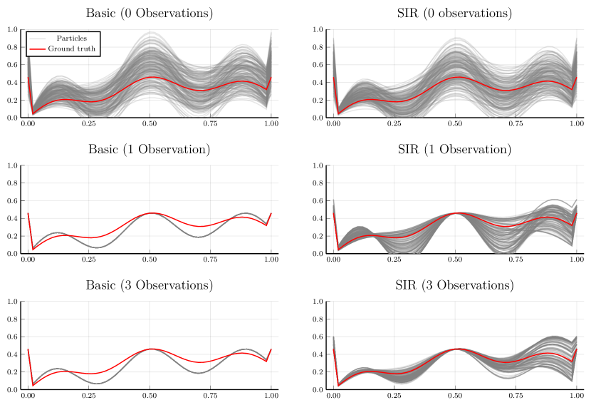
Figure 2: Comparison between basic particle filtering (left column) and SIR (right column) after different numbers of observations.

Appendix C Experiment Hyperparameters

The parameters for the POMDP formulation and the hyperparameters for the experimental setup are included in table 2.

Table 2: POMDP and Solver Hyperparameters

Variable Description	Value
Discount Factor ($\gamma$)	$0.9$
$\lambda_{\rm leaked}$	$-1000.0$
$\lambda_{\rm exited}$	$-1000.0$
$\lambda_{\rm trapped}$	$100.0$
$\lambda_{\rm obs}$	$-0.1$
CO2 height std. dev. ($\sigma_{\rm height}$)	$0.01$
CO2 thickness std. dev. ($\sigma_{\rm sat}$)	$0.01$
Observation configurations	$\{0.25\!:\!0.25\!:\!0.75,0.125\!:\!0.125\!:\!0.875\}$
Injection rates	$\{0.01,0.07\}$
Drill Locations	$\{0.1\!:\!0.1\!:\!0.9\}$
Distribution of $h_{\rm lobe}$	$\mathcal{U}(0.05,0.25)$
Distribution of $h_{\rm center}$	$\mathcal{U}(0.05,0.5)$
Distribution of $h_{\rm elev}$	$\mathcal{U}(0.05,0.5)$
Distribution of normalized porosity ($\rho$)	$\mathcal{U}(0.5,1.5)$
Exploration Coefficient for UCB	$20.0$
Observation widening exponent ($\alpha_{\rm obs})$	$0.3$
Observation widening coefficient ($k_{\rm obs})$	$10.0$
Action widening exponent ($\alpha_{\rm act}$)	$0.5$
Action widening coefficient ($k_{\rm act})$	$10.0$
Number of tree queries ($N_{\rm query}$)	$5000$
Estimation value for leaf nodes	$0.1\times$ optimal return
Particles for Basic Particle filter	$2000$
Particles for SIR ($N$)	$200$
Samples per iteration for SIR	$100$
Max CPU time for belief update	$60$ seconds

References

- [1] Hans-Otto Pörtner et al. “Climate change 2022: Impacts, adaptation and vulnerability” In IPCC Sixth Assessment Report IPCC Geneva, The Netherlands, 2022
- [2] International Energy Agency “World Energy Outlook 2020”, 2020, pp. 464 DOI: https://doi.org/https://doi.org/10.1787/557a761b-en
- [3] Sally M. Benson and Franklin M. Orr “Carbon dioxide capture and storage” In MRS Bulletin 33.4 Cambridge University Press, 2008, pp. 303–305
- [4] Bert Metz et al. “IPCC special report on carbon dioxide capture and storage” Cambridge: Cambridge University Press, 2005
- [5] Tabbi Wilberforce et al. “Outlook of carbon capture technology and challenges” In Science of the total environment 657 Elsevier, 2019, pp. 56–72
- [6] International Energy Agency “CCUS in Clean Energy Transitions”, 2020 IEA Paris
- [7] Mykel J. Kochenderfer, Tim A. Wheeler and Kyle H. Wray “Algorithms for Decision Making” MIT Press, 2022
- [8] Céline Scheidt, Lewis Li and Jef Caers “Quantifying uncertainty in subsurface systems” John Wiley & Sons, 2018
- [9] Dan Lu, Scott Painter, Nicholas Azzolina and Matthew Burton-Kelly “Accurate and timely forecasts of geologic carbon storage using machine learning methods” In NeurIPS Workshop on Tackling Climate Change with Machine Learning, 2021
- [10] Obiajulu J. Isebor, Louis J. Durlofsky and David E. Ciaurri “A derivative-free methodology with local and global search for the constrained joint optimization of well locations and controls” In Computational Geosciences 18.3 Springer, 2014, pp. 463–482
- [11] Yun Yang et al. “A niched Pareto tabu search for multi-objective optimal design of groundwater remediation systems” In Journal of Hydrology 490 Elsevier, 2013, pp. 56–73
- [12] Giorgio De Paola, Cristina Ibanez-Llano, Jesus Rios and Georgios Kollias “Reinforcement learning for field development policy optimization” In SPE Annual Technical Conference and Exhibition, 2020 OnePetro
- [13] Yizheng Wang et al. “A sequential decision-making framework with uncertainty quantification for groundwater management” In Advances in Water Resources 166 Elsevier, 2022, pp. 104266
- [14] Halvor Møll Nilsen, Knut-Andreas Lie, Olav Møyner and Odd Andersen “Spill-point analysis and structural trapping capacity in saline aquifers using MRST-co2lab” In Computers and Geosciences 75, 2015, pp. 33–43 DOI: https://doi.org/10.1016/j.cageo.2014.11.002
- [15] Zachary N Sunberg and Mykel J Kochenderfer “Online algorithms for POMDPs with continuous state, action, and observation spaces” In International Conference on Automated Planning and Scheduling, 2018