Spatiotemporal control of active topological defects

Topological defects play a central role in the physics of many materials, including magnets, superconductors and liquid crystals. In active fluids, defects become autonomous particles that spontaneously propel from internal active stresses and drive chaotic flows stirring the fluid. The intimate connection between defect textures and active flow suggests that properties of active materials can be engineered by controlling defects, but design principles for their spatiotemporal control remain elusive. Here we provide a symmetry-based additive strategy for using elementary activity patterns, as active topological tweezers, to create, move and braid such defects. By combining theory and simulations, we demonstrate how, at the collective level, spatial activity gradients act like electric fields which, when strong enough, induce an inverted topological polarization of defects, akin to an exotic negative susceptibility dielectric. We harness this feature in a dynamic setting to collectively pattern and transport interacting active defects. Our work establishes an additive framework to sculpt flows and manipulate active defects in both space and time, paving the way to design programmable active and living materials for transport, memory and logic.

The ability to manipulate matter at the nano, micro and mesoscale is essential for developing functional materials with adaptive and responsive properties  (?). A common strategy is to employ repetitive assembly of discrete physical units (e.g., polymers, colloids, elastic beams etc.) to construct (meta)materials that acquire novel morphologies and functionalities from their architecture  (?, ?, ?, ?, ?). When rationally designed, such structured materials exhibit unconventional mechanical responses  (?), enable programmable computation in materia  (?, ?) and mimic living systems  (?). But this approach doesn’t apply to continuous media. Taking inspiration from solid-state magnetic memories that use magnetic domain walls as mobile bits  (?, ?), an alternate strategy is to employ topological defects of an ordered phase as information-carrying building blocks of a hierarchical material. Topological defects are characteristic singularities that emerge when ordered phases of matter are obtained through a rapid quench or are frustrated by boundaries and external fields  (?). By virtue of being discrete excitations, defects bridge the gap between the analog and the digital, encoding information of the continuous order parameter in robustly localized singularities that behave as effective quasiparticles. From manipulating magnetic skyrmions  (?, ?) and superconducting vortices  (?, ?) to knotting disclination loops in liquid crystals  (?, ?, ?), the control of defects in diverse systems offers new opportunities for designing reconfigurable memories and logic devices.

Topological defects also naturally emerge in active fluids  (?, ?, ?), i.e., fluids composed of self-driven units such as bacteria, motor protein-biofilament constructs, active colloids and living cells  (?, ?, ?, ?, ?) that can organize into states with (nematic) liquid crystalline order. Active nematic fluids ubiquitously develop spontaneous flows driven by self-propelled defects  (?, ?, ?) that chaotically self-stir the fluid  (?, ?, ?). The intimate feedback between distortions of order, dynamical defects and flow (Fig. 1A) makes active fluids an attractive platform for manipulating transport of matter, energy and information far from equilibrium  (?, ?, ?). Global control of active flows have been achieved by imposing constraints via geometry, confinement, substrates, etc.  (?, ?, ?, ?, ?, ?). More recent experimental advances in optically responsive platforms now allow local spatiotemporal control of internal stresses in bacterial and synthetic active fluids  (?, ?, ?, ?, ?, ?) enabling unprecedented abilities to sculpt and configure active materials on demand. Complementing these experimental results, recent theoretical works have also begun exploring the inverse problem in the context of optimal control  (?, ?), reinforcement learning  (?) and pattern formation  (?, ?, ?, ?).

Yet a rational design framework to control active topological defects is lacking, begging the question - how can we construct spatiotemporal profiles of active stresses to dynamically control active defects and flow (Fig. 1A)? We systematically solve this inverse problem by developing a symmetry-based additive approach (Fig. 1) that focuses on active defects as the primary drivers of flow in the system and exploits the linearity of inertia-less dynamics. Elementary defects in 2D nematics are disclinations characterized by a topological winding number $\nu=\pm 1/2$ (Fig. 1B)  (?). In addition, $\pm 1/2$ defects are also distinguished by the geometry of their local nematic texture; comet-shaped $+1/2$ defects have a polarity captured by a unit vector $\hat{{\bf e}}$ (Fig. 1B, left), while triangular $-1/2$ defects have a three-fold symmetry captured by a unit complex triatic parameter $\Theta_{3}$ (Fig. 1B, right)  (?, ?); see Methods and SI for details. The dynamics of defects is obtained from the hydrodynamics of an active fluid which is modeled as a thin, two dimensional (2D) viscous layer characterized by a nematic order parameter ${\bf Q}$ and flow velocity ${\bf u}$ whose coupled dynamics is governed by Stokesian force balance and passive relaxation, which give  (?, ?, ?)

$$\partial_{t}{\bf Q}+{\bf u}\cdot\bm{\nabla}{\bf Q}={\bf S}({\bf u},{\bf Q})+\dfrac{1}{\gamma}{\bf H}\;,$$ (1)

$$-\Gamma{\bf u}+\eta\nabla^{2}{\bf u}-\bm{\nabla}\Pi+\bm{\nabla}\cdot\left(\bm{\sigma}^{a}+\bm{\sigma}^{el}\right)={\bf 0}\;.$$ (2)

Local order is advected, rotated and sheared by flow (captured by ${\bf S}({\bf u},{\bf Q})$, see Methods for details) and distortions relax via the molecular field ${\bf H}=(a_{2}-a_{4}\mathrm{tr}[{\bf Q}^{2}]){\bf Q}+K\nabla^{2}{\bf Q}$ ($a_{2,4}>0$) with elasticity $K$ and rotational viscosity $\gamma$ (Eq. 1). Force balance (Eq. 2) includes damping from viscosity ($\eta$) and friction ($\Gamma$), pressure $\Pi$ enforcing incompressibility ($\bm{\nabla}\cdot{\bf u}=0$), an elastic stress $\bm{\sigma}^{el}$ (see Methods for details) and an active stress $\bm{\sigma}^{a}=\alpha{\bf Q}$  (?), where the activity $\alpha$ captures the average strength of the oriented force dipoles exerted by the active units on the fluid ($\alpha<0$: extensile, $\alpha>0$: contractile). Importantly, activity $\alpha({\bf r},t)$ varies in space and time, serving as the control variable and we focus on the extensile case ($\alpha<0$) relevant for most experimental systems  (?, ?) (though our results hold more generally). In the following we work in units such that the nematic correlation length $\xi=\sqrt{K/a_{2}}=1$, the nematic relaxation time $\tau_{n}=\gamma/a_{2}=1$, and a passive elastic stress scale $K\Gamma/\gamma=1$

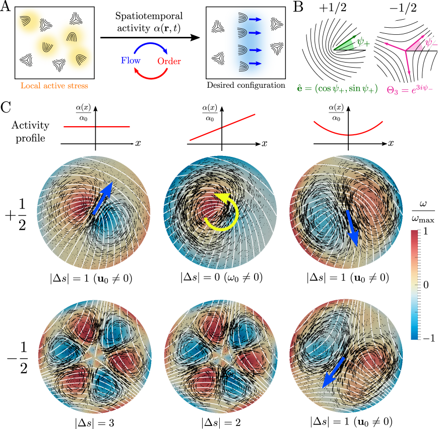
Figure 1: Additive framework for spatiotemporal control of active defects. (A) Active stresses generate flow through distortions of order in active nematic fluids resulting in the proliferation of motile defects. How can we locally actuate active stresses to achieve desired defect textures and flow patterns in space-time? (B) Disclinations with topological charge $\nu=\pm 1/2$ have distinct symmetries characterized by a vector $\hat{{\bf e}}$ ($+1/2$) and a complex triatic parameter $\Theta_{3}$ ($-1/2$). (C) In the vicinity of a defect (director, white lines), simple polynomial activity profiles (constant: left, linear: middle, quadratic: right) in space locally generate distinct flow (${\bf u}$, black arrows) and vorticity ($\omega=\hat{{\bf z}}\cdot(\bm{\nabla}\times{\bf u})$, heat map) fields, here computed using Eq. 2 with a screening length $\ell_{\eta}=\sqrt{\eta/\Gamma}=2\xi$ and no-slip boundary conditions. The nature of the flow velocity and vorticity at the defect core (${\bf u}_{0}$, blue arrow; $\omega_{0}$, yellow arrow) is dictated by the combined rotational symmetry of the defect texture ($s$) and the activity pattern ($n$) quantified by the absolute index difference $|\Delta s|=|s-n|$. Linear combinations of individual activity patterns simply sum the respective flow fields providing an additive strategy for generating arbitrarily complex active flows.

As any distortion of order generates flow in an active fluid (Eq. 2), defects self-generate local active flows that advect and rotate them  (?, ?, ?). By assuming a separation of timescales wherein nematic distortions relax faster than the dynamics of defects  (?, ?, ?), we can neglect the nonlinearity in Eq. 1. Thus to control the trajectory of an individual defect described by $3$ independent degrees of freedom (DoFs, two translational, one rotational), we need to prescribe the local flow velocity ${\bf u}_{0}$ and vorticity $\omega_{0}$ actively generated at the defect core. But the control parameter, the activity $\alpha({\bf r},t)$, is a single scalar field with effectively infinite DoFs. To overcome this DoF mismatch, reminiscent of similar problems in neuromotor control  (?), we turn to symmetry.

In the simple case of constant activity, it is well-known that $+1/2$ defects self-propel along their polarity with nonzero flow at their core (${\bf u}_{0}^{+}\propto\alpha\hat{{\bf e}}$) while three-fold symmetric $-1/2$ defects do not (${\bf u}_{0}^{-}={\bf 0}$)  (?, ?), highlighting the importance of defect rotational symmetry for its motion. For a generic activity profile, because the active stress $\bm{\sigma}^{a}$ is bilinear in activity ($\alpha$, the control) and the nematic texture (${\bf Q}$, the state), the combined symmetry of the two fields dictates the nature of local flow. Euclidean isometries of the plane that leave the origin (defect core) fixed are characterized by the orthogonal group $\mathsf{O}(2)$ and all its discrete dihedral subgroups $\mathsf{D}_{n}$ (i.e., the symmetries of an $n$-sided regular polygon). We thus expand the activity in terms of angular Fourier harmonics ($\alpha({\bf r})=\sum_{n}\tilde{\alpha}_{n}(r)e^{in\phi}$, $\phi$ is the polar angle) which offer a natural basis with definite $n$-fold dihedral symmetry. The rotational symmetry of 2D nematic defects can be similarly quantified. Defect textures with topological winding $\nu$ can be assigned an integer symmetry index $s=2|1-\nu|$  (?) corresponding to their dihedral symmetry group $\mathsf{D}_{s}$. As expected, $+1/2$ defects have $s=1$ and $-1/2$ defects have $s=3$.

Figure 2: Active topological tweezers enable complex manipulation of defect paths. (A-C) Moving a $-1/2$ defect using an active tweezer; see Movie S1 (path shown in A). (B) The $-1/2$ defect (magenta triangle) tracks the motion of a small activation disc (dashed circle) with a centered quadrupolar activity profile (see Methods and SI for details) whose orientation controls the local flow and direction of motion. $(\Delta x,\Delta y)$ denote distance from the core of the controlled defect. (C) Tracked trajectory of $-1/2$ defect shaded by the normalized time $t/T$ ($T$ is the protocol duration). (D-F) Moving a $+1/2$ defect using an active tweezer; see Movie S2 (path shown in D). (E) The $+1/2$ defect (green arrow) tracks the motion of a small activation disc (dashed circle) with a centered quadrupolar activity profile (see Methods and SI for details). (C) Tracked trajectory of $+1/2$ defect shaded by normalized time $t/T$. (G) Demonstration of simultaneous multidefect control using active tweezers, with defect pair creation (filled circles, left), braided trajectories and pair exchange (arrows, left), ending in pair annihilation (crosses, left); see Movie S3. An elliptic localized patch of high activity allows local nucleation of $\pm 1/2$ defect pairs (right, zoomed-in snapshot). (H) Tracked trajectory of defects ($+1/2$: green, $-1/2$: magenta) forms a closed braid, the figure-eight ($4_{1}$) knot, in space-time. (I) Snapshots showing defect braiding in time.

To obtain a finite defect velocity or vorticity (${\bf u}_{0},\omega_{0}\neq 0$), the angle average (zeroth angular moment) of the respective fields must be nonvanishing. Linearity of Eq. 2 and the form of the active stress $\bm{\sigma}^{a}$ then prescribe a simple selection rule (see Theorem 1 in Methods for proof): for a defect with symmetry $s$ subjected to an $n$-fold symmetric activity profile (only $\tilde{\alpha}_{\pm n}\neq 0$), a necessary condition for self-propulsion (${\bf u}_{0}\neq 0$) is $|s-n|=1$, and for self-rotation ($\omega_{0}\neq 0$) is $|s-n|=0$ (see Fig. 1C). While symmetry dictates the existence (or not) of local active flow, its specific form and direction depend on details of the activity pattern and defect orientation. An explicit calculation of ${\bf u}_{0}$, $\omega_{0}$ for $\pm 1/2$ defects in a smoothly varying activity profile yields (see Methods for details)

$${\bf u}_{0}^{+}=\bm{\mathcal{V}}_{+}\cdot\hat{{\bf e}}\;,\quad\omega_{0}^{+}=\hat{{\bf z}}\cdot\left(\bm{\Omega}_{+}\bm{\times}\hat{{\bf e}}\right)\;,$$ (3)

$${\bf u}_{0}^{-}=\left(\mathrm{Re}[\Theta_{3}\mathcal{V}_{-}],\,\mathrm{Im}[\Theta_{3}\mathcal{V}_{-}]\right)\;,\quad\omega_{0}^{-}=-\mathrm{Re}[i\Theta_{3}\Omega_{-}]\;,$$ (4)

where (to leading order in gradients) $\bm{\mathcal{V}}_{+}\propto\alpha{\bf I}+\mathcal{O}(\nabla^{2}\alpha)$, $\mathcal{V}_{-}\propto\partial^{2}\alpha$ ($\partial=(\partial_{x}-i\partial_{y})/2$), $\bm{\Omega}_{+}\propto\bm{\nabla}\alpha$ and $\Omega_{-}\propto\partial^{3}\alpha$ are translational and rotational response coefficients that depend linearly on the local activity and its symmetry mandated gradients evaluated at the defect core (see Methods for details). In Eqs. 3, 4, we have simply Taylor-expanded the activity near the defect core upon assuming weak spatial gradients. Flows generated by $\pm 1/2$ defects in elementary polynomial profiles of activity are shown in Fig. 1C. Strikingly, we see that while linear gradients of activity ($\bm{\nabla}\alpha\neq{\bf 0}$; $n=1$ symmetry) only contribute to vorticity of $+1/2$ defects, consistent with  (?, ?, ?), quadratic activity gradients ($\bm{\nabla}\bm{\nabla}\alpha\neq{\bf 0}$; $n=2$ symmetry) generate net active flow for both $\pm 1/2$ defects (Fig. 1C) as predicted by the symmetry selection rule. Arbitrary linear combinations of activity patterns then simply superpose their respective flow fields thereby providing an attractive additive and modular strategy for designing complex local flows from active defects.

We now deploy our design framework in numerical simulations of Eqs. 1, 2 (see Methods and SI for details) to construct activity patterns for basic defect based operations. For controlling individual defects, we generalize “topological tweezers”  (?) used in colloidal crystals to devise active topological tweezers (Fig. 2), i.e., a disc of finite activity, whose motion and local spatiotemporal pattern is chosen to achieve a prescribed defect transport task. The selection rule dictates that a quadrupolar activity profile ($\tilde{\alpha}_{\pm 2}\neq 0$) is the simplest pattern that can translate $\pm 1/2$ defects in different directions (see Methods and Extended Data Figs. 1-2). We illustrate this idea by using an active tweezer with a time-varying quadrupolar activity profile to move a $-1/2$ defect along a bent trajectory (Fig. 2A-C, Movie S1). A $90^{\circ}$ rotation of the profile causes the $-1/2$ defect to move in an orthogonal direction. A $+1/2$ defect can also be moved along a similar trajectory using a different active tweezer profile (Fig. 2D-F, Movie S2). In both cases, the defect successfully tracks the motion of the tweezer (Fig. 2C and F) for a range of disc speeds $V$ that are comparable or smaller than the activity induced speed $|{\bf u}_{0}|$, i.e., $V\leq|{\bf u}_{0}|$, but very rapid disc motion ($V\gg|{\bf u}_{0}|$) leaves the defect behind, see SI and Extended Data Figs. 3-4 for details.

More complex defect manipulations are also possible. As an example, we implement an active tweezer based protocol for simultaneous mulidefect control and use it to accomplish a nontrivial defect exchange and braiding task (Fig. 2G-I, Movie S3). In a uniformly ordered nematic, we nucleate two pairs of $\pm 1/2$ defects using a high activity ramp within a localized elliptic patch that controls the initial orientation of the defect pair created (Fig. 2G, right). After the defect pairs are separated, the $-1/2$ defects are braided around each other using active tweezers and finally annihilated with the $+1/2$ defect from the opposite pair, accomplishing pair exchange (Fig. 2G, I; Movie S3). Although defects also experience elastic forces due to distortions of the nematic  (?), the local active forces are sufficiently strong to overcome any elastic interaction.The world lines of the four defects, from creation to annihilation, trace out a closed braid with four crossings forming the figure eight ($4_{1}$) knot in space-time (Fig. 2H), which is the simplest, yet nontrivial, achiral prime knot. Notably, unlike active nematics with homogeneous activity, where the spontaneous motility of $+1/2$ defects alone drives autonomous braiding of defect trajectories  (?), our example in Fig. 2G-I demonstrates braiding of the usually disregarded $-1/2$ defect. Active tweezers hence generate patterned flows that enable control of arbitrarily complex braided and knotted trajectories for both $\pm 1/2$ defects. These capabilities suggest potential strategies for controlling local fluid mixing  (?, ?) and provide key steps towards developing reconfigurable space-time assemblies of active defects for programmable logic devices  (?, ?).

Having demonstrated the capability for controlling individual or a few defects, we extend our framework to address multidefect control at the collective level. To do so, we need to account for two additional features. The first is elastic forces between defects that take the form of Coulomb interactions, familiar from passive liquid crystal physics  (?). The second is the well known propensity of active nematics to develop chaotic flows and active turbulence (for sufficiently high activity, $|\alpha|\gg K\Gamma/\gamma$), accompanied by swirling $\pm 1/2$ defect pairs that spontaneously unbind and proliferate  (?, ?). In the regime of many such unbound defects, a coarse-grained hydrodynamic approach for the defect gas is warranted. Following previous work by some of us  (?, ?), we develop effective defect hydrodynamic equations that average over fluctuations on the scale of the mean defect spacing and the defect lifetime to describe the distribution of $\pm 1/2$ defects in terms of smoothly varying fields such as their respective densities $\rho_{\pm}({\bf r},t)=\langle\sum_{i}\delta[{\bf r}-{\bf r}^{\pm}_{i}(t)]\rangle$ (${\bf r}^{\pm}_{i}$ is the position of the $i$th $\pm 1/2$ defect; see Methods). A key advance over Ref.  (?) is the inclusion of both a polarization field ${\bf p}({\bf r},t)=\langle\sum_{i}\hat{{\bf e}}_{i}\delta[{\bf r}-{\bf r}^{+}_{i}(t)]\rangle$ and a complex triatic order parameter $T_{3}({\bf r},t)=\langle\sum_{i}\Theta_{3}^{i}\delta[{\bf r}-{\bf r}^{-}_{i}(t)]\rangle$ to capture collective orientational ordering of $\pm 1/2$ defects due to spatial activity gradients (see Methods for details). We derive defect hydrodynamics by coarse-graining effective active particle-like dynamics for $\pm 1/2$ defects (see SI for details) that combine activity gradient induced motility and rotations from Eqs. 3, 4 with passive elastic interactions and active collective torques (similar to previously derived torques in Refs.  (?, ?)). Defect interaction forces and torques are mediated by nematic distortions quantified by the smoothed phase gradient ${\bf v}_{n}=\langle\bm{\nabla}\theta\rangle$, where $\theta$ is the local nematic orientation (see Methods for details).

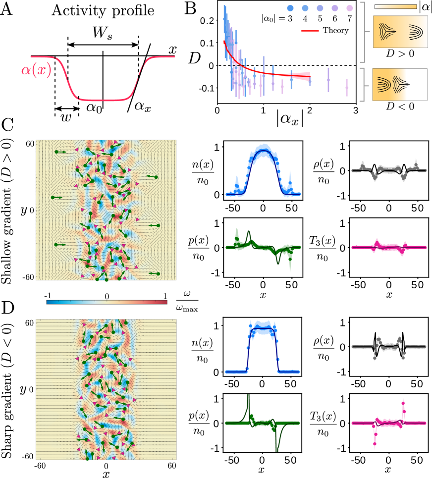
Figure 3: Collective spatial patterning of defects realizes charge dipole inversion. (A) A 1D active strip of width $W_{s}=50$ with an extensile activity profile $\alpha(x)<0$ that smoothly connects the maximal activity $\alpha_{0}$ in the interior of the strip to zero outside. In the interfacial region, the activity varies as a sigmoid over a width $w$, generating an activity gradient $\alpha_{x}\sim\alpha_{0}/w$. (B) Topological dipole moment ($D$) quantifies interfacial charge separation as a function of activity gradient ($\alpha_{x}$) for different $\alpha_{0}$, $w$ (dots: numerical simulation, error bar is one standard deviation). The model (Eqs. 5-7) quantitatively predicts the dipole flip transition (red line using $|\alpha_{0}|=5$, shaded region is one standard deviation using an $N=10$ bootstrap subsample; see SI for details). (C-D) The dynamical steady state for shallow ($w=40$, C) and sharp ($w=15$, D) activity gradients (both with $|\alpha_{0}|=5$) with snapshots shown (left) and spatial defect distributions quantified (right) comparing simulations (dots, shaded region is one standard deviation) with theory (lines, see SI for details).

For a static activity profile $\alpha(x)$ varying in 1D, at steady-state we can set $\rho_{\pm}=\rho_{\pm}(x)$, ${\bf p}=p(x)\hat{{\bf x}}$, ${\bf v}_{n}=v_{n}(x)\hat{{\bf y}}$ etc. (see Methods for details). Neglecting any nonlinear buildup of defect order and expanding to lowest order in gradients, the hydrodynamic equations governing collective flux balance for the $\pm 1/2$ defect orientations and their velocities then reduce to (see Methods for details)

$$-\dfrac{1}{\tau_{R}}p-\dfrac{1}{2}\partial_{x}(\rho_{+}\mathcal{V}_{+})-\dfrac{1}{2}\rho_{+}\Omega_{+}+\mu_{R}\mathcal{V}_{+}\rho_{+}\;v_{n}=0\;,$$ (5)

$$-\dfrac{1}{\tau_{R}}T_{3}-\dfrac{1}{2}\partial_{x}(\rho_{-}\mathcal{V}_{-})+\mu_{R}\mathcal{V}_{-}\rho_{-}\;v_{n}=0\;,$$ (6)

$$p\mathcal{V}_{+}-T_{3}\mathcal{V}_{-}+2\mu Kn\;v_{n}=0\;,$$ (7)

where the 1D response coefficients $\mathcal{V}_{\pm}(x)$, $\Omega_{+}(x)$ (Eqs. 3, 4) are spatial functions of activity (see Methods for details), $\tau_{R}$ is a defect reorientation time and $\mu_{R}$ (dimensionless) and $\mu\propto 1/\gamma$ are rotational and translational defect mobilities respectively (see Methods for details). The average defect density $n=(\rho_{+}+\rho_{-})/2$ is controlled by a steady balance of defect creation and annihilation with $n(x)\propto|\alpha(x)|$  (?) (see SI for details) and the charge density $\rho=(\rho_{+}-\rho_{-})/2$ is simply obtained from the conservation of topological charge via Gauss’ law: $2\pi\rho(x)=\partial_{x}v_{n}(x)$  (?). Note, Eq. 7 balances the motility ($\mathcal{V}_{\pm}$) of both $\pm 1/2$ defects with elastic forces ($\sim\mu Knv_{n}$) to set the topological charge current to zero in steady state. Eqs. 5-7 then allow us to compute the spatial distribution of defects in a given 1D activity profile.

To validate and test our theoretical predictions, we perform numerical simulations of the full nematodynamic model (Eqs. 1, 2) using different activity patterns. For simple activity profiles such as a linear or quadratic gradient, we can analytically solve Eqs. 5-7 and obtain quantitative fits for $n(x)$, $\rho(x)$, $p(x)$, $T_{3}(x)$ (see SI for details). With the phenomenological parameters of our defect hydrodynamic model (Eqs. 5-7) in hand, we now challenge our model using a more complex activity profile consisting of an active strip of width $W_{s}=50$ flanked by passive regions (Fig. 3A). Within the active strip, the maximal activity ($\alpha_{0}$) is always chosen to be well in the regime of active turbulence. Near the interface, the activity varies in a sigmoidal fashion allowing us to tune the interfacial activity gradient ($\alpha_{x}\equiv\mathrm{d}\alpha/\mathrm{d}x|_{W_{s}/2}\sim\alpha_{0}/w$) and the width of the interface ($w$) independently (Fig. 3A).

For shallow gradients ($|\alpha_{x}|\leq 0.2$), the motile $+1/2$ defects escape and accumulate out of the strip, leaving behind $-1/2$ defects on the inside (Fig. 3C, left; Movie S4). As a result, the interface develops a topological charge dipole as the activity gradient behaves as an “electric field” separating defects by topological charge. This effect, first predicted in Ref.  (?), simply relies on the fact that $+1/2$ defects behave like active particles, which accumulate where they move slowly, and disregards the negligible propulsion of $-1/2$ defects in weak gradients ($\mathcal{V}_{-}\ll\mathcal{V}_{+}$, see Methods and SI for details). Remarkably, for sharp activity gradients ($|\alpha_{x}|\geq 0.2$), we find a different behavior, wherein the $+1/2$ defects are no longer able to tunnel through the interface, and $-1/2$ defects instead accumulate near the edge of the strip (Fig. 3D left; Movie S5). Similar effects have been noted previously for individual defects  (?, ?), but not at the collective level. To quantify the charge separation of defects, we compute a steady state dipole moment $D=(1/2)\int\mathrm{d}x\;|x|\rho(x)$ and plot it as a function of the interfacial activity gradient $|\alpha_{x}|$ (Fig. 3B). Upon varying both the maximal activity ($|\alpha_{0}|$) and the interfacial width ($w$), we find a common trend, i.e., when the activity gradient $|\alpha_{x}|$ is increased, the dipole moment switches from $D>0$ (excess $+1/2$ defects on the low activity side) to $D<0$ (excess $+1/2$ defects on the high activity side), see Fig. 3B. Note that, as $|\alpha_{0}|\gg 1$ (above the active turbulence threshold), the dipole moment remains nonvanishing even for arbitrarily weak gradients ($|\alpha_{x}|\to 0$, $w\to\infty$). Following the electrostatic analogy, the active nematic behaves as an unusual polarizable medium with a nonlinear response such that for shallow activity gradients (‘weak field’) the system behaves as a conventional dielectric, whereas for sharp activity gradients (‘strong field’), the system displays a negative static susceptibility, a feature forbidden at equilibrium  (?).

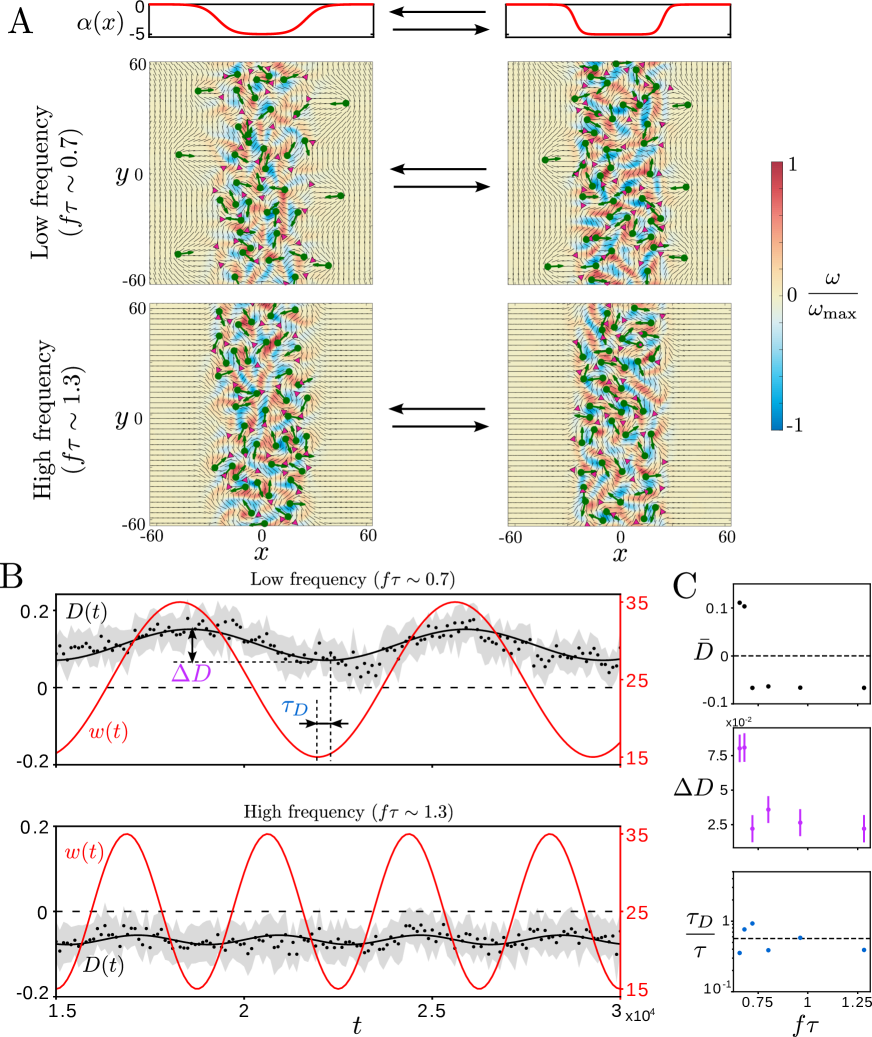
Figure 4: Dynamic response of active defects to oscillatory gradients. (A) The interfacial width ($w$) is varied sinusoidally and its oscillation frequency ($f$) controls defect organization. (B) The dynamical steady state is quantified by a periodic dipole moment $D(t)$ (dots: simulation with shaded region as one standard deviation, black line: sinusoidal fit) which switches from overall $D(t)>0$ at low frequencies ($f\tau\sim 0.7$, top) to $D(t)<0$ at higher frequencies ($f\tau\sim 1.3$, bottom). The time trace of the imposed interfacial width ($w(t)$) is shown in red. (C) The sinusoidal fit (with frequency $f$) of the time varying dipole moment shows how the average value ($\bar{D}$, top), amplitude of oscillation ($\Delta D$, middle) and time delay ($\tau_{D}$, bottom) vary as a function of drive frequency ($f$).

How can we understand the inversion of the dipole moment? While previous simpler treatments are unable to predict this phenomenon  (?), by accounting for the active propulsion and rotation of both $\pm 1/2$ defects, our improved defect hydrodynamic model (Eqs. 5-7) quantitatively captures this dipole flip transition without any fitting parameters (Fig. 3B, red line using $|\alpha_{0}|=5$; see SI for details). We next compare the numerically measured spatial distributions of defect density ($n$), charge density ($\rho$) and orientational order parameters ($p$, $T_{3}$) with our model predictions, with qualitatively comparable results overall (Fig. 3C-D, right). The average defect density $n(x)$ is well predicted in both cases ($n_{0}$ is the maximal defect density in the center) and features of charge separation ($\rho(x)$) and $+1/2$ polarization ($p(x)$) are qualitatively captured for shallow gradients (Fig. 3C, right; see SI for details). But the model predictions for spatial profiles are less accurate for sharp gradients (Fig. 3D, right), where $p(x)$ is overestimated and $T_{3}(x)$ is underestimated (see SI for details). We attribute the lack of quantitative accuracy in the spatial profile predictions to the neglect of higher gradient and nonlinear terms that affect the defect density and cause saturation of defect order, particularly for strong activity gradients (see SI for details). Nonetheless, some general features are apparent. Intuitively, the sharp activity interface acts like a virtual wall that blocks the motion of defects through it, as noted previously in simulations  (?) and experiments  (?, ?). In a thin boundary layer near the edge of the active strip, the locally strong activity gradient causes $-1/2$ defects to self-propel faster than $+1/2$ defects ($\mathcal{V}_{-}\geq\mathcal{V}_{+}$), but both $\pm 1/2$ defects rapidly lose their motility upon crossing the interface. Similar boundary layers have been recently observed at confining walls as well  (?). As a result, $-1/2$ defects get preferentially trapped along the interface, preventing any $+1/2$ defects from crossing the interface, thus realizing the inverted dipole state.

The resulting charge dipole is accompanied by a interfacial defect ordering and a change in the nematic orientation outside the active strip as well. As shown in Fig. 3C-D, while shallow activity gradients cause the nematic to orient parallel to the interface (due to the escaped $+1/2$ defects whose polarization points down activity gradients), a sharp interface forces the nematic to reorient perpendicular to the interface (due to ordered $-1/2$ defects). Our results demonstrate that defect decorated activity interfaces display tunable ‘active anchoring’  (?) that allow control of collective defect organization and nematic orientation simply via the strength of the local activity gradient.

We now employ the active strip as a defect patterning motif in a dynamic setting. As shallow interfaces are leaky to the escape of $+1/2$ defects, but sharp interfaces are not, we ask if periodically oscillating the interface width allows us to dynamically control the organization of active defects. We fix $|\alpha_{0}|=5$ and vary the interface width sinusoidally in time (with frequency $f$) between values $w_{\mathrm{min}}=15$ and $w_{\mathrm{max}}=35$ (Fig. 4A), so that the average width ($\bar{w}=25$) corresponds to an almost vanishing dipole moment ($D\approx 0$) in the static limit (see Fig. 3B). The average time $\tau=\bar{w}^{2}/D_{a}$ it takes $+1/2$ defects to cross the interface with an active diffusion constant $D_{a}=\langle|{\bf u}_{0}|^{2}\rangle\tau_{R}/2\sim 0.82$ (see SI for details) sets a characteristic time scale that controls the dynamic response. At low oscillation frequencies ($f\tau\sim 0.7$, with $\tau\sim 765$), $+1/2$ defects have sufficient time to escape through the shallow interface and remain trapped in the passive region when the interface becomes sharp (Fig. 4A, Movie S6). As a result, the system develops a steady-state dipole moment that is always positive ($D(t)>0$) and oscillates in sync with the interface (Fig. 4B, top), albeit with a time delay ($\tau_{D}$, Fig. 4B-C).

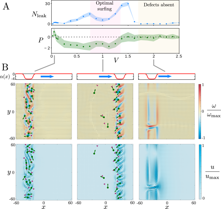
Figure 5: Collective transport of active defects by ‘surfing’. (A) A 1D active strip ($|\alpha_{0}|=4$, $W_{s}=20$, $w=10$) moving with speed $V$ can be used to collectively transport active defects. Transport efficacy is quantified by the total number of defects that leak out of the strip ($N_{\mathrm{l}eak}$, blue dots) and the total polarization of $+1/2$ defects ($P$, green dots). The blue and green shaded regions represent one standard deviation. Few defects are lost for $V\ll 1$ but the transport is slow, whereas for very high speeds ($V\gg 1$, yellow shaded region), the strip moves faster than defects can nucleate. Only at intermediate speeds ($V\sim 1$, shaded red region) do we obtain optimal defect surfing, where few defects are left behind and the $+1/2$ defects develop significant collective polarization ($|P|\gg 1$). (B) Snapshots show the three characteristic regimes for $V\ll 1$ (left), $V\sim 1$ (middle) and $V\gg 1$ (right) with both vorticity ($\omega$) and flow speed ($u=|{\bf u}|$) plotted.

For a higher driving frequency ($f\tau\sim 1.3$), $+1/2$ defects have insufficient time to escape and they get dynamically trapped to the active strip (Fig. 4A, Movie S7). The system then dynamically realizes an inverted dipole state with $D(t)<0$ (Fig. 4B, bottom). We quantify this dynamic transition by performing a sinusoidal fit of the steady-state dipole moment and plot the time-averaged dipole moment ($\bar{D}$), the amplitude of oscillations ($\Delta D$) and the time delay in the response ($\tau_{D}$) as a function of the driving frequency $f$ (Fig. 4C). While $\bar{D}$ and $\Delta D$ show stronger variation upon increasing frequency (with $\bar{D}$ switching sign), the average time delay $\tau_{D}\sim 0.6\tau$ is intrinsic to the active defect gas and does not vary systematically with the drive (Fig. 4C).

Along with defect patterning, another basic task is defect transport. As a simple example, we use a 1D moving active strip (with speed $V$) to illustrate how active defects can be collectively transported in space. For simplicity, we fix the maximal activity $|\alpha_{0}|=4$ and choose the strip geometry to have sharp interfaces ($W_{s}=20$, $w=10$) to ensure defects are trapped to the active region when the strip is stationary. To achieve rapid and efficient transport, it is natural to consider large $V$, but fast motion of the active strip can cause defects to be left behind, despite the sharp interfaces. To quantify this trade-off we compute (in steady-state) the total number of defects that escape and leak out of the active strip ($N_{\mathrm{leak}}$, Fig. 5A) and the net horizontal polarization of all the $+1/2$ defects ($P=\int\mathrm{d}{\bf r}\;p$, Fig. 5A).

For slow speeds ($V\ll 1$) the transport time is long but the defects remain largely localized to the active region ($N_{\mathrm{leak}}\sim 0$) with no net polarization ($P\sim 0$) as they follow the travelling strip adiabatically (Fig. 5B left, Movie S8). For very rapid motion of the strip ($V\gg 1$, shaded yellow region in Fig. 5A), there is insufficient time to nucleate and carry defects (Fig. 5B right; Movie S10). Only for intermediate speeds ($V\sim 1$, shaded red region in Fig. 5A) do we obtain optimal collective transport of defects characterized by an enhanced carrying capacity (decrease in $N_{\mathrm{leak}}$, Fig. 5A) and significant $+1/2$ polarization ($|P|\gg 1$, Fig. 5A). In this regime, the active strip moves at a speed comparable to the activity induced propulsion of the defects, allowing the defects to collectively ‘surf’ the imposed travelling wave of activity, and organize the otherwise turbulent interior of the active strip into a state with spatially patterned flow and vortices (Fig. 5B middle, Movie S9).

In this work, we have demonstrated how topological defects offer robust particle-like excitations that can be functionally controlled to manipulate continuous active fluids in space and time. Our symmetry based additive framework enables the construction of active topological tweezers for basic defect operations that provide the basis of complex computation and logic in a fluidic system  (?, ?). By extending the framework to incorporate defect interactions, we developed a coarse-grained hydrodynamic description of active defects at the collective level, enabling the characterization of large-scale patterning and dynamics of the defect gas. Activity gradients are shown to behave as “electric fields” that segregate defects by charge and topologically polarize the active fluid, albeit with unusual responses that mimic certain dielectric metamaterials. Complementing the spatial response, we also probe the dynamic response of defects and highlight simple strategies for patterning and transporting large collections of active defects.

Our work provides a general framework to control and rationally design active materials as metafluids for soft microrobotics  (?, ?) and defect based soft logic  (?, ?). Current experiments on light-controlled active fluids  (?, ?, ?) offer a natural platform to deploy our control strategies. Beyond engineered systems, active defects have been identified in biological tissues and cellular monolayers, and proposed to act as sites of biological function and morphogenesis  (?, ?, ?, ?). Our work suggests that a similar symmetry based approach can be used to understand how active defects get functionalized in biological systems, paving the way for controlling and designing defect based autonomous materials from living matter with adaptive and programmable functionality.

Data Availability

Code used for the numerical simulations is available on https://github.com/LVDScharrer/ATC. All other data needed to reproduce the results in this paper are provided in the Methods and Supplementary Information.

Materials and Methods

Here we provide details of the hydrodynamic model, the numerical simulations and the analytical calculations for the active flows below.

1 Active nematodynamics

The orientational order of the active nematic in 2D is locally characterized by an alignment tensor $Q_{ij}=S(\hat{n}_{i}\hat{n}_{j}-\delta_{ij}/2)$ with the director $\hat{{\bf n}}=(\cos\theta,\sin\theta)$, where $S$ is the scalar order parameter and $\theta$ refers to the director angle. A continuum hydrodynamic description of the 2D active nematic film is given by (Eqs. 1, 2)

$$\partial_{t}{\bf Q}+{\bf u}\cdot\bm{\nabla}{\bf Q}={\bf S}({\bf u},{\bf Q})+\dfrac{1}{\gamma}{\bf H}\;,$$ (8)

$$-\Gamma{\bf u}+\eta\nabla^{2}{\bf u}-\bm{\nabla}\Pi+\bm{\nabla}\cdot\left(\bm{\sigma}^{a}+\bm{\sigma}^{el}\right)={\bf 0}\;,$$ (9)

with the molecular field ${\bf H}=(a_{2}-a_{4}\mathrm{tr}[{\bf Q}^{2}]){\bf Q}+K\nabla^{2}{\bf Q}$ ($a_{2,4}>0$). Note here we have already assumed the system prefers an ordered nematic phase in the absence of activity. Without loss of generality, we set $a_{4}=a_{2}$. Then the equilibrium ground state is an ordered homogeneous nematic with $S=S_{0}=2$. The flow coupling ${\bf S}({\bf u},{\bf Q})$ is given by  (?)

$$S_{ij}=Q_{ik}W_{kj}-W_{ik}Q_{kj}+\lambda E_{ij}+\lambda(E_{ik}Q_{kj}+Q_{ik}E_{kj}-\delta_{ij}Q_{k\ell}E_{k\ell})-2\lambda Q_{k\ell}E_{k\ell}Q_{ij}\;,$$ (10)

where $\lambda$ is the flow-alignment parameter ($|\lambda|>1$ for flow-aligning systems), $E_{ij}=(\partial_{i}u_{j}+\partial_{j}u_{i})/2$ is the strain-rate tensor (purely deviatoric as $\bm{\nabla}\cdot{\bf u}=0$), and $W_{ij}=(\partial_{i}u_{j}-\partial_{j}u_{i})/2$ is the vorticity tensor.

The active stress is $\bm{\sigma}^{a}=\alpha{\bf Q}$  (?) and the passive liquid-crystal stress is given by

$$\sigma^{el}_{ij} =Q_{ik}H_{kj}-H_{ik}Q_{kj}-K\partial_{i}Q_{kl}\partial_{j}Q_{kl}$$

$$\quad+\lambda(2Q_{ij}+\delta_{ij})Q_{kl}H_{kl}-\lambda H_{ik}\left(Q_{kj}+\dfrac{1}{2}\delta_{kj}\right)-\lambda\left(Q_{ik}+\dfrac{1}{2}\delta_{ik}\right)H_{kj}\;.$$ (11)

The pressure $\Pi$ enforces incompressibility ($\bm{\nabla}\cdot{\bf u}=0$) and is calculated from the pressure Poisson equation obtained by taking the divergence of Stokes’ equation (Eq. 9):

$$\nabla^{2}\Pi=\partial_{i}\partial_{j}\left(\sigma^{el}_{ij}+\sigma^{a}_{ij}\right)$$ (12)

We note that only symmetric components of $\bm{\sigma}^{el}$ will contribute to the pressure, due to the symmetry of the $\partial_{i}\partial_{j}$ operator.

1.1 Numerical simulations

In order to numerically simulate the nematodynamic equations, we nondimensionalize Eqs. 8, 9. As mentioned in the main text, we employ the nematic coherence length $\xi=\sqrt{K/a_{2}}$ as our unit of length, the elastic relaxation time $\tau_{n}=\gamma/a_{2}$ as our unit of time, and a passive stress scale $K\Gamma/\gamma$ as our unit of stress. We are then left with four nondimensionless parameters: $\tilde{\ell}_{\eta}=\ell_{\eta}/\xi$, $\tilde{\gamma}=\gamma/\eta$, $\tilde{\alpha}=\alpha\gamma/(K\Gamma)$ and $\lambda$. The topological tweezer demonstrations were performed with $\tilde{\ell}_{\eta}=5$, chosen to display flow patterns more clearly, while the collective effect simulations were performed at a lower viscosity $\tilde{\ell_{\eta}}=\sqrt{5}$, to increase defect density and improve the statistics of defect averages. For all simulations, we set $\tilde{\gamma}=0.1$ and $\lambda=1.8$.

Numerical simulations of the continuum nematodynamic equations (Eqs. 8, 9) were performed with a custom Matlab code using a second order pseudospectral time-exponentiation scheme for numerical integration, on a lattice of $256\times 256$ gridpoints with periodic boundary conditions. We used a grid spacing of $\mathrm{d}x=0.5$ and timestep $\mathrm{d}t=0.1$. The $-1/2$ and $+1/2$ tweezer demonstrations in Fig. 2 were run for a total of $1,520$ and $1,800$ timesteps respectively, while the braiding procedure was run for $6,500$ timesteps. The dipole moment datapoints reported in Fig. 3 were computed using $N=40$ independent simulations, each running for $10^{5}$ timesteps. The data for oscillating activity gradients (Fig. 4) were computed using $N=6$ independent simulations, each run for $3\times 10^{5}$ timesteps, and the demonstrations with traveling activity patterns (Fig. 5) were run for $5\times 10^{4}$ timesteps. All simulations were performed on an NVIDIA GeForce GTX 1060 Mobile graphics card, and we estimate that each $10^{4}$ timesteps of simulation time corresponded to a wall-clock runtime of $\sim 12$ minutes, resulting in a typical overall runtime of $\sim 150$ hours.

2 Defect dynamics in spatial activity patterns

In this section, we compute the flows generated by topological defects in the presence of spatially varying activity profiles. We provide the details of the additive framework for controlling individual defects and the formulation of the defect hydrodynamic model.

2.1 Structure and flow of isolated active defects

The 2D orientational order of the active nematic is locally characterized by an alignment tensor $Q_{ij}=S(2\hat{n}_{i}\hat{n}_{j}-\delta_{ij})$ with director $\hat{{\bf n}}=(\cos\theta,\sin\theta)$. An isolated $\pm 1/2$ defect at the origin is described by $\theta=\pm\phi/2+\theta_{0}$, where $\phi$ is the polar angle and $\theta_{0}$ dictates the orientation of the defect. The scalar order parameter $S$ is taken to be constant ($S=S_{0}$) outside the core of the defect ($r\geq a$, $a$ is the core size). The orientation of a $+1/2$ defect is captured by a unit vector  (?, ?)

$$\hat{{\bf e}}={\lim_{r\rightarrow 0}\dfrac{\bm{\nabla}\cdot\mathbf{Q}}{|\bm{\nabla}\cdot\mathbf{Q}|}}=(\cos\psi_{+},\sin\psi_{+})\;,\quad\psi_{+}=2\theta_{0}\;.$$ (13)

On the other hand, the orientation of the three-fold symmetric $-1/2$ defect is more complicated and described by a rank three symmetric tensor $\Theta_{ijk}$ given by  (?)

$$\Theta_{ijk}=\lim_{r\to 0}\dfrac{\langle\partial_{i}Q_{jk}+\partial_{j}Q_{ik}+\partial_{k}Q_{ij}\rangle}{3|\langle\partial_{k}Q_{ij}\rangle|}=\hat{t}_{i}\hat{t}_{j}\hat{t}_{k}-\dfrac{1}{4}\left[\delta_{ij}\hat{t}_{k}+\delta_{kj}\hat{t}_{i}+\delta_{ik}\hat{t}_{j}\right]\;,$$ (14)

$$\hat{{\bf t}}=(\cos\psi_{-},\sin\psi_{-})\;,\quad\psi_{-}=\dfrac{2\theta_{0}}{3}\;,$$ (15)

where $\langle\cdot\rangle$ is an angular average around the defect core. One can check that $\Theta_{ijk}$ vanishes if any two indices are contracted. As a result, $\Theta_{ijk}$ only has two independent components ($\Theta_{xxx}=-\Theta_{xyy}=(1/4)\cos 3\psi_{-}$, $\Theta_{yyy}=-\Theta_{xxy}=-(1/4)\sin 3\psi_{-}$), and an alternate representation that we will use interchangeably is the triatic complex parameter $\Theta_{3}=e^{3i\psi_{-}}$.

The flow generated by the defect is computed using Stokes equation (Eq. 9). As the nematic texture of an isolated defect is an equilibrium solution, both the molecular field and the elastic stress (Eq. 11) vanishes, i.e., ${\bf H}={\bf 0}$ and $\bm{\sigma}^{el}={\bf 0}$. Stokes equation then simplifies and the flow generated by the active stress $\bm{\sigma}^{a}=\alpha{\bf Q}$ is computed from

$$\ell_{\eta}^{2}\nabla^{2}{\bf u}-{\bf u}+\dfrac{1}{\Gamma}\bm{\nabla}\cdot\bm{\sigma}^{a}-{\dfrac{1}{\Gamma}}\bm{\nabla}\Pi=0\;,\quad\bm{\nabla}\cdot{\bf u}=0\;,$$ (16)

where we have used the hydrodynamic screening length $\ell_{\eta}=\sqrt{\eta/\Gamma}$. Incompressibility is enforced by using a 2D stream function, ${\bf u}=-\hat{{\bf z}}\times\bm{\nabla}\Psi$ ($u_{x}=\partial_{y}\Psi\,,u_{y}=-\partial_{x}\Psi$), so the vorticity $\omega={\hat{{\bf z}}\cdot}(\bm{\nabla}\times{\bf u})=-\nabla^{2}\Psi$ satisfies

$$\ell_{\eta}^{2}\nabla^{2}\omega-\omega+\dfrac{1}{\Gamma}\mathcal{W}=0\;,$$ (17)

where $\mathcal{W}={\hat{{\bf z}}\cdot}(\bm{\nabla}\times\bm{\nabla}\cdot\bm{\sigma}^{a})$ is the rotational component of the active force density. For a $\pm 1/2$ defect, we will denote the corresponding stream-function as $\Psi^{\pm}$, the flow as ${\bf u}^{\pm}$ and the vorticity as $\omega^{\pm}$.

Defects behave like quasiparticles driven by self-generated active flows at their core  (?, ?). Following similar analysis previously performed for the case of both homogeneous activity  (?, ?, ?, ?) and simple gradient profiles  (?), we compute the active flow and vorticity near the core of a $\pm 1/2$ defect defined as

$${\bf u}^{\pm}_{0}=\lim_{r\to a}\int_{0}^{2\pi}\dfrac{\mathrm{d}\phi}{2\pi}{\bf u}^{\pm}(r,\phi)=\int_{0}^{2\pi}\dfrac{\mathrm{d}\phi}{2\pi}\left(\sin\phi,-\cos\phi\right)\left.\left(\partial_{r}\Psi^{\pm}+\dfrac{\Psi^{\pm}}{r}\right)\right|_{r=a}\;,$$ (18)

$$\omega_{0}^{\pm}=\lim_{r\to a}\int_{0}^{2\pi}\dfrac{\mathrm{d}\phi}{2\pi}\;\omega^{\pm}(r,\phi)\;,$$ (19)

where we have integrated by parts and used the fact that $u_{x}=(1/r)\cos\phi\partial_{\phi}\Psi+\sin\phi\partial_{r}\Psi$ and $u_{y}=(1/r)\sin\phi\partial_{\phi}\Psi-\cos\phi\partial_{r}\Psi$. From Eqs. 18, 19 we directly see that only the zeroth angular harmonic (i.e., constant in $\phi$) of $\omega^{\pm}$ (or equivalently $\Psi^{\pm}$) contributes to the defect rotation rate $\omega_{0}^{\pm}$, and only the first angular harmonic of $\omega^{\pm}$ and $\Psi^{\pm}$ contributes to the defect velocity ${\bf u}_{0}^{\pm}$.

2.2 General proof of the selection rule

Here we provide a proof for the symmetry-based selection rule that underlies the additive control framework and the construction of active topological tweezers.

An arbitrary activity pattern $\alpha({\bf r})$ can be expanded in an angular Fourier basis,

$$\alpha({\bf r})=\sum_{n=-\infty}^{\infty}\tilde{\alpha}_{n}(r)\;e^{in\phi}\;,$$ (20)

where $\phi$ is polar angle and $\tilde{\alpha}_{n}(r)$ are complex functions ($\tilde{\alpha}^{*}_{n}=\tilde{\alpha}_{-n}$) of the distance $r$ from the defect core. Note that $n$ characterizes the ($n$-fold) rotational symmetry of the activity profile. We can similarly expand the stream-function and vorticity in an angular Fourier basis as

$$\Psi({\bf r})=\sum_{n=-\infty}^{\infty}\tilde{\Psi}_{n}(r)\;e^{in\phi}\;,\quad\omega({\bf r})=\sum_{n=-\infty}^{\infty}\tilde{\omega}_{n}(r)\;e^{in\phi}\;.$$ (21)

We shall now prove the following general theorem whose corollary is the desired selection rule.

Theorem 1.

Consider an isolated defect with topological charge $\nu$ and flow ${\bf u}$ satisfying linear Stokes equation (Eq. 16). Suppose the flow has $\tilde{\Psi}_{m}(r)\neq 0$ for some $m\in\mathbb{Z}$, then $\exists\;\tilde{\alpha}_{n}(r)\neq 0$ that generates $\tilde{\Psi}_{m}(r)$, if and only if $n\in\mathbb{Z}$ satisfies the equation $|m|=|2-n-2\nu|$.

Proof.

As Stokes equation (Eq. 9) is linear, we can perform an angular Fourier transform and the different Fourier modes decouple. Eq. 17 simplifies to give,

$$\ell_{\eta}^{2}\left[\tilde{\omega}_{n}^{\prime\prime}+\dfrac{1}{r}\tilde{\omega}_{n}^{\prime}-\dfrac{n^{2}}{r^{2}}\tilde{\omega}_{n}\right]-\tilde{\omega}_{n}+\dfrac{1}{\Gamma}\tilde{\mathcal{W}}_{n}=0\;,$$ (22)

$$\tilde{\Psi}_{n}^{\prime\prime}+\dfrac{1}{r}\tilde{\Psi}_{n}^{\prime}-\dfrac{n^{2}}{r^{2}}\tilde{\Psi}_{n}=-\tilde{\omega}_{n}\;.$$ (23)

It is convenient to write the curl of the active force density $\mathcal{W}=\hat{{\bf z}}\cdot(\bm{\nabla}\times\bm{\nabla}\cdot\bm{\sigma}^{a})$ in complex form as follows

$$\mathcal{W}=\mathrm{Re}\left[-i\left(\partial_{x}^{2}-\partial_{y}^{2}-2i\partial_{x}\partial_{y}\right)\left(\sigma^{a}_{xx}+i\sigma^{a}_{xy}\right)\right]\;.$$ (24)

Using the fact that $Q_{xx}+iQ_{xy}=S_{0}e^{2i(\nu\phi+\theta_{0})}$ for an isolated defect texture with charge $\nu$, we have for a spatially varying $\alpha$ (Eq. 20)

$$\sigma^{a}_{xx}+i\sigma^{a}_{xy}=S_{0}\sum_{n=-\infty}^{\infty}\tilde{\alpha}_{n}(r)\;e^{i[(2\nu+n)\phi+2\theta_{0}]}\;.$$ (25)

From Eq. 24, we then obtain the angular Fourier mode $\tilde{\mathcal{W}}_{m}(r)=\int_{0}^{2\pi}(\mathrm{d}\phi/2\pi)\;e^{-im\phi}\mathcal{W}({\bf r})$ to be

$$\tilde{\mathcal{W}}_{m} =i\dfrac{S_{0}}{2}\left[-e^{2i\theta_{0}}\left(\tilde{\alpha}_{n}^{\prime\prime}+\dfrac{(3+2m)}{r}\tilde{\alpha}^{\prime}_{n}+\dfrac{m(m+2)}{r^{2}}\tilde{\alpha}_{n}\right)\delta_{m,-2+n+2\nu}\right.$$

$$\quad\left.+e^{-2i\theta_{0}}\left(\tilde{\alpha}_{-n}^{\prime\prime}+\dfrac{(3-2m)}{r}\tilde{\alpha}^{\prime}_{-n}+\dfrac{m(m-2)}{r^{2}}\tilde{\alpha}_{-n}\right)\delta_{m,2-n-2\nu}\right]\;.$$ (26)

From Eq. 26, we immediately see that $\tilde{\mathcal{W}}_{m}\neq 0$ only for $m=\pm(2-n-2\nu)$. By linearity of Stokes equation (Eq. 22, 23), $\tilde{\Psi}_{m}\neq 0\iff\tilde{\mathcal{W}}_{m}\neq 0$ and from Eq. 26, $\tilde{\mathcal{W}}_{m}\neq 0\iff\tilde{\alpha}_{n}\neq 0$ for some $\tilde{\alpha}_{n}(r)$ with $|m|=|2-n-2\nu|$. This concludes the proof. ∎

We now use Theorem 1 to obtain the selection rule. In terms of the angular Fourier moments, the angle averaged flow and vorticity at the defect core (Eqs. 18, 19) simplify to

$$u_{0x}+iu_{0y}=-i\left.\left(\tilde{\Psi}_{-1}^{\prime}+\dfrac{1}{r}\tilde{\Psi}_{-1}\right)\right|_{r=a}\;,\quad\omega_{0}=\tilde{\omega}_{0}|_{r=a}\;.$$ (27)

As we are interested in the translations and rotations of the defect, we only need to focus on and compute $\tilde{\Psi}_{0}$ and $\tilde{\Psi}_{-1}$ in terms of the $\alpha$ to obtain the active flow and vorticity at the defect core. So we only consider the cases $|m|=1$ and $|m|=0$ in the Theorem 1 and obtain the required selection rule.

To simplify notation, it is more transparent and easier to use the symmetry of the defect rather than the charge. For a 2D nematic disclination with topological charge $\nu$, the rotational symmetry ($s$) of the defect texture is related to the charge by  (?)

$$s=2|1-\nu|\;.$$ (28)

As expected, a $\nu=+1/2$ defect is polar or $1$-fold symmetric ($s=1$), a $\nu=-1/2$ defect is $3$-fold symmetric ($s=3$), a $\nu=+1$ vortex is isotropic ($s=0$) and a $\nu=-1$ antivortex is $4$-fold symmetric ($s=4$).

Combining Theorem 1 with Eqs. 27, 28, we can finally state the symmetry selection rule in compact form as follows.

Symmetry selection rule: Consider an isolated defect in 2D with topological charge $\nu$ and rotational symmetry $s>0$ subject to an activity pattern $\alpha({\bf r})$ with an $n$-fold symmetric component, i.e., $\tilde{\alpha}_{\pm n}(r)\neq 0$ ($n>0$). Then a necessary condition for

• activity-induced flow velocity at the core (${\bf u}_{0}\neq{\bf 0}$) is $|n-s|=1$, and

• activity-induced vorticity at the core ($\omega_{0}\neq 0$) is $|n-s|=0$.

For this condition to be sufficient as well, the radial profile of $\tilde{\alpha}_{n}(r)$ must not be homogeneous solution of Eq. 26.

2.3 Topological tweezer construction

Here we sketch simple designs for topological tweezers. The are three main constraints to satisfy - (i) the selection rule for the symmetry of the activity pattern, (ii) the maximum activity is smaller than the bend-instability threshold and (iii) $\alpha$ does not change sign (so the system never switches from extensile to contractile or vice-versa). To reduce the effort of actuation, we minimize gradients in activity, so we choose radially constant activity profiles as far as we can and choose the smallest angular variation required to satisfy the symmetry rule. These design principles allow the construction of simple topological tweezers for translating $\pm 1/2$ defects.

To translate either $\pm 1/2$ defect, the symmetry rule dictates that we need atleast an $n=2$-fold symmetric activity pattern. For a $+1/2$ defect, even the isotropic ($n=0$) activity pattern will generate propulsion. A simple choice for $\alpha$ (centered on the defect) is then

$$\alpha({\bf r})=\begin{cases}\alpha_{0}[1+A\sin(2\phi)+B\cos(2\phi)]\quad(r\leq R)\\ 0\quad(r>R)\end{cases}\;,$$ (29)

so $\tilde{\alpha}_{0}=\alpha_{0}$ and $\tilde{\alpha}_{\pm 2}=(\alpha_{0}/2)(B\mp iA)$. $\alpha_{0}<0$ dictates the maximum extensile activity and $\sqrt{A^{2}+B^{2}}\leq 1$ to maintain fixed sign of $\alpha$. To compute the active flow generated by either $\pm 1/2$ defect, we have to solve Eq. 16 in the plane with appropriate far-field boundary conditions ($|{\bf u}|\to 0$ as $|{\bf r}|\to\infty$). As $\alpha$ is discontinuous across $r=R$ (the tweezer boundary, see Eq. 29), the vorticity-streamfunction approach adopted above is technically cumbersome as the active vorticity source $\mathcal{W}$ is highly singular at $r=R$ (see Eq. 26). We instead adopt a simpler solution by using the Green’s function for Eq. 16 to write ${\bf u}({\bf r})=\int\mathrm{d}{\bf r}^{\prime}{\bf G}({\bf r}-{\bf r}^{\prime})\cdot[\bm{\nabla}^{\prime}\cdot\bm{\sigma}^{a}({\bf r}^{\prime})]$, where  (?)

$$G_{ij}({\bf r})=\dfrac{1}{2\pi\eta}\left[G_{1}\left(\dfrac{r}{\ell_{\eta}}\right)\delta_{ij}+\dfrac{r_{i}r_{j}}{r^{2}}G_{2}\left(\dfrac{r}{\ell_{\eta}}\right)\right]\;,$$ (30)

$$G_{1}(z)=-\dfrac{1}{z^{2}}+\dfrac{1}{2}[K_{0}(z)+K_{2}(z)]\;,$$ (31)

$$G_{2}(z)=\dfrac{2}{z^{2}}-K_{2}(z)\;,$$ (32)

where $K_{n}(z)$ are modified Bessel functions of the second kind.

The flow velocity at the core is then obtained by integrating by parts and setting ${\bf r}={\bf 0}$, which gives $u_{i}({\bf 0})=-\int\mathrm{d}{\bf r}^{\prime}\;\partial^{\prime}_{k}G_{ij}({\bf r}^{\prime})\sigma^{a}_{jk}({\bf r}^{\prime})$. The integral can be easily performed as $\bm{\sigma}^{a}$ is nonsingular everywhere. Upon simplifying, we obtain the core velocity for both $\nu=\pm 1/2$ defects to be

$${\bf u}_{0}^{+}=\dfrac{v_{0}}{4}\left(\vphantom{\dfrac{A}{A}}(2f_{1}+Bf_{2})\cos 2\theta_{0}+Af_{2}\sin 2\theta_{0},Af_{2}\cos 2\theta_{0}+(2f_{1}-Bf_{2})\sin 2\theta_{0}\right)\;,$$ (33)

$${\bf u}_{0}^{-}=\dfrac{v_{0}}{4}f_{1}\left(\vphantom{\dfrac{A}{A}}B\cos 2\theta_{0}+A\sin 2\theta_{0}\;,-A\cos 2\theta_{0}+B\sin 2\theta_{0}\right)\;,$$ (34)

where the overall self-propulsion speed is given by $v_{0}=|\alpha_{0}|S_{0}/\Gamma R$ (for $\alpha_{0}<0$) and the constants $f_{1,2}$ are given by

$$f_{1}=-\dfrac{R}{\ell_{\eta}}\int_{a/\ell_{\eta}}^{R/\ell_{\eta}}\mathrm{d}z\;zK_{1}(z)\;,$$ (35)

$$f_{2}=\dfrac{R}{\ell_{\eta}}\int_{a/\ell_{\eta}}^{R/\ell_{\eta}}\mathrm{d}z\left[-\dfrac{8}{z^{2}}+zK_{3}(z)\right]\;.$$ (36)

Here $a$ is the finite defect core size. Note, $f_{1,2}$ remain finite in the $a/\ell_{\eta}\to 0$ limit. In the opposite (friction dominated) limit where $\ell_{\eta}\to 0$, the defect core size ($a>0$) must be retained as a short-distance cutoff.

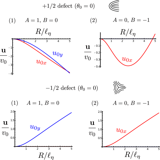
Extended Data Figure 1: Flow generated by topological tweezers. The active flow velocity at the defect core (${\bf u}_{0}$, Eqs. 33, 34; solid curves) is plotted as a function of $R/\ell_{\eta}$ ($R$: tweezer radius, $\ell_{\eta}$: screening length) for both $\pm 1/2$ defects using the activity profile given in Eq. 29 with different values of $A,B$. The defect core size is set to $a=0$ and the defect orientation is taken to be horizontal with $\theta_{0}=0$ (as shown in the schematics). The flow is normalized by the bare self-propulsion speed $v_{0}=|\alpha_{0}|S_{0}/\Gamma R$ and its $x$ (red) and $y$ (blue) components are separately plotted (components not shown vanish). Nonzero $A$ allows flows along the y-axis for both defects, perpendicular to the defect orientation. Changing the sign of $A$ flips the direction of $u_{0y}$. Flows along the x-axis depend on $B$ and the screening length $\ell_{\eta}$. All examples use $A^{2}+B^{2}=1$ to obtain maximal effect of activity gradients.

Extended Data Figure 2: Comparing numerical and theoretical flows generated by topological tweezers. The active flow velocity at the defect core (${\bf u}_{0}$) is numerically computed for a $+1/2$ (top) and $-1/2$ (bottom) defect by solving Stokes’ equation (Eq. 16) in a periodic box of size $2L=128$ with a ${\bf Q}$ tensor corresponding to an ideal isolated defect with $\theta_{0}=0$ and an activity pattern for a tweezer (Eq. 29) with $\alpha_{0}=-1$, $A=0$ and $B=-1$. The tweezer radius ($R$) and screening length ($\ell_{\eta}$) are separately varied as shown in the legend. The angle averaged flow velocity (x-component: left, y-component: right) at the origin is nondimensionalized by $v_{0}=|\alpha_{0}|S_{0}/\Gamma R$ and plotted for both the numerical solution (solid curves) and the analytical prediction (Eqs. 33, 34 with core size $a=1$; dashed curves). For both defects, $u_{y}$ is theoretically predicted to be zero, but the numerical solution obtains a small but nonvanishing transverse flow. The numerical curves for $u_{x}$ are similarly qualitatively consistent with the theory prediction. We attribute the quantitative discrepancy between the curves to the periodic boundary conditions and details of the defect core that are neglected in the theory calculation.

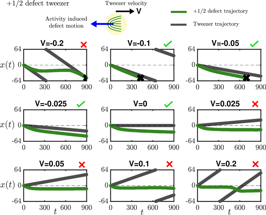
Extended Data Figure 3: Characterizing the $+1/2$ topological tweezer. A tweezer of size $R=12$ and activity profile in Eq. 29 with parameters $\alpha_{0}=-1.5$, $A=0$, $B=0$ is chosen to move a $+1/2$ defect ($\theta_{0}=0$). The screening length $\ell_{\eta}=5$. The activity induced defect motion is in the $-\hat{x}$ direction (speed $\sim 0.1$) and the tweezer disc is itself moved along the x-axis with a velocity $V$ ($V>0$: right moving, $V<0$: left moving). The defect tracks (green line) the tweezer motion (gray line) when the tweezer speed is smaller or equal to the activity induced motion ($-0.1\lesssim V\leq 0$, panels marked by green ticks). When the tweezer moves too fast ($V<-0.1$) or moves in the opposite direction to the active motion ($V>0$), the defect quickly leaves the active region of the tweezer (after a time $\sim R/V$) and fails to track the tweezer motion (panels marked by red crosses). In some cases, the tweezer trajectory wraps around due to periodic boundary conditions and causes a small displacement of the defect when the tweezer passes over. Black crosses terminating some defect trajectories represent points where the $+1/2$ defect annihilated with a $-1/2$ defect present at the same location.

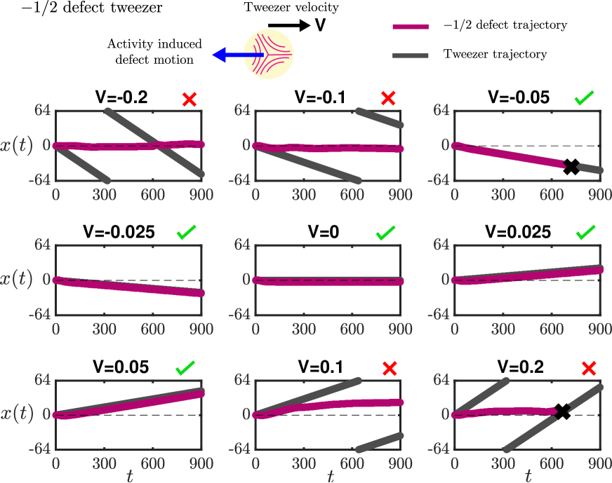
Extended Data Figure 4: Characterizing the $-1/2$ topological tweezer. A tweezer of size $R=12$ and activity profile in Eq. 29 with parameters $\alpha_{0}=-5$, $A=0$, $B=-1$ is chosen to move a $-1/2$ defect ($\theta_{0}=0$). The screening length $\ell_{\eta}=5$. The activity induced defect motion is in the $-\hat{x}$ direction (speed $\sim 0.05$) and the tweezer disc is itself moved along the x-axis with a velocity $V$ ($V>0$: right moving, $V<0$: left moving). The defect tracks (magenta line) the tweezer motion (gray line) when the tweezer speed is smaller or equal to the activity induced motion ($|V|\lesssim 0.05$, panels marked by green ticks). When the tweezer moves too fast in either direction ($|V|>0.05$), the defect quickly leaves the active region of the tweezer (after a time $\sim R/V$) and fails to track the tweezer motion (panels marked by red crosses). Unlike the $+1/2$ tweezer shown in Extended Data Fig. 3, the $-1/2$ defect can be dragged by an active tweezer even in a direction opposite to its activity induced motion, as long as the tweezer speed is small enough. In some cases, the tweezer trajectory wraps around due to periodic boundary conditions and causes a small displacement of the defect when the tweezer passes over. Black crosses terminating some defect trajectories represent points where the $-1/2$ defect annihilated with a $+1/2$ defect present at the same location.

2.4 Defect velocity and vorticity for polynomial activity

Here we consider a special case of the more general result in Sec. 2.2 by focusing on polynomial activity profiles. In the vicinity of a defect (assumed at the origin), we Taylor expand the activity profile in powers of the distance ${\bf r}$ from the core as

$$\alpha({\bf r})=\alpha_{0}+\alpha_{i}r_{i}+\dfrac{1}{2}\alpha_{ij}r_{i}r_{j}+\dfrac{1}{6}\alpha_{ijk}r_{i}r_{j}r_{k}+\mathcal{O}(r^{4})\;,$$ (37)

where $\alpha_{0}=\alpha({\bf 0})$, $\alpha_{i}=\partial_{i}\alpha({\bf 0})$, and so on. In terms of the angular Fourier moments (Eq. 20), we have the following nonvanishing terms

$$\tilde{\alpha}_{0}(r)=\alpha_{0}+\dfrac{r^{2}}{4}\alpha_{kk}+\mathcal{O}(r^{4})\;,$$ (38)

$$\tilde{\alpha}_{1}(r)=\dfrac{r}{2}(\alpha_{x}-i\alpha_{y})+\dfrac{r^{3}}{16}\left[\alpha_{xxx}+\alpha_{xyy}-i\left(\alpha_{xxy}+\alpha_{yyy}\right)\right]+\mathcal{O}(r^{5})\;,$$ (39)

$$\tilde{\alpha}_{2}(r)=\dfrac{r^{2}}{8}\left(\alpha_{xx}-\alpha_{yy}-2i\alpha_{xy}\right)+\mathcal{O}(r^{4})\;,$$ (40)

$$\tilde{\alpha}_{3}(r)=\dfrac{r^{3}}{48}\left[\alpha_{xxx}-3\alpha_{xyy}+i\left(\alpha_{yyy}-3\alpha_{xxy}\right)\right]+\mathcal{O}(r^{5})\;.$$ (41)

Solving Eq. 26 with $m=0,1$ for both $\nu=\pm 1/2$ defects, we obtain (to lowest nontrivial order in activity gradients)

$$\tilde{\mathcal{W}}^{+}_{0}=\dfrac{3S_{0}}{2r}\alpha_{i}\epsilon_{ij}\hat{e}_{j}+\mathcal{O}(r)\;,$$ (42)

$$\tilde{\mathcal{W}}^{+}_{1}=-i\dfrac{S_{0}}{2}\left(-\dfrac{\alpha_{0}}{r^{2}}+\dfrac{3}{4}\alpha_{kk}\right)e^{-2i\theta_{0}}-i\dfrac{15S_{0}}{16}\left(\alpha_{xx}-\alpha_{yy}-2i\alpha_{xy}\right)e^{2i\theta_{0}}+\mathcal{O}(r^{2})\;,$$ (43)

$$\tilde{\mathcal{W}}^{-}_{0}=-r\dfrac{5S_{0}}{4}\Theta_{ijk}\epsilon_{k\ell}\alpha_{ij\ell}+\mathcal{O}(r^{3})\;,$$ (44)

$$\tilde{\mathcal{W}}^{-}_{1}=\dfrac{3S_{0}}{4}\left[\Theta_{yjk}\alpha_{jk}+i\Theta_{xjk}\alpha_{jk}\right]+\mathcal{O}(r^{2})\;,$$ (45)

where $\epsilon_{ij}$ is the antisymmetric Levi-Civita tensor and we have used the $+1/2$ defect polarization $\hat{{\bf e}}=(\cos 2\theta_{0},\sin 2\theta_{0})$ along with the $-1/2$ defect triatic parameter $\Theta_{ijk}$.

To solve for the stream function $\Psi$ and the flow ${\bf u}$, we need to specify boundary conditions. As we have Taylor expanded $\alpha$, we only solve Eq. 17 in a finite circular domain of radius $R$ and enforce no-slip boundary conditions along the boundary, i.e., ${\bf u}|_{r=R}={\bf 0}$. For simplicity, we work in the friction dominated regime ($\ell_{\eta}\to 0$) and neglect viscous dissipation (finite $\ell_{\eta}$ only changes things quantitatively as shown in Sec. 2.3). In this limit, Eq. 17 simplifies to $\omega=\mathcal{W}/\Gamma$. Solving for the stream function and setting $\partial_{\phi}\Psi|_{r=R}=\partial_{r}\Psi|_{r=R}=0$, we obtain for the $n=-1$ angular harmonic mode,

$$\tilde{\Psi}_{-1}^{+}(r) =-i\dfrac{\alpha_{0}S_{0}R}{4r\Gamma}\left(1-\dfrac{r}{R}\right)^{2}e^{2i\theta_{0}}-\mathcal{A}\dfrac{S_{0}R^{3}}{6r\Gamma}\left(1+\dfrac{2r}{R}\right)\left(1-\dfrac{r}{R}\right)^{2}\;,$$ (46)

$$\tilde{\Psi}_{-1}^{-}(r) =\dfrac{3S_{0}}{4\Gamma}\left[\dfrac{r^{2}}{3}-\dfrac{Rr}{2}+\dfrac{R^{3}}{6r}\right]\left(-\Theta_{yjk}\alpha_{jk}+i\Theta_{xjk}\alpha_{jk}\right)\;,$$ (47)

where $\mathcal{A}=(-3i/16)[2\alpha_{kk}e^{2i\theta_{0}}-5(\alpha_{xx}-\alpha_{yy})e^{-2i\theta_{0}}-10i\alpha_{xy}e^{-2i\theta_{0}}]$. The angularly averaged vorticity is simply given by $\tilde{\mathcal{W}}_{0}$ in the $\ell_{\eta}\to 0$ limit, so we have

$$\tilde{\omega}_{0}^{+}(r) =\dfrac{3S_{0}}{2\Gamma r}\;\alpha_{i}\epsilon_{ij}\hat{e}_{j}\;,$$ (48)

$$\tilde{\omega}_{0}^{-}(r) =-r\dfrac{5S_{0}}{4\Gamma}\Theta_{ijk}\epsilon_{k\ell}\alpha_{ij\ell}\;.$$ (49)

Using these solutions for $\omega^{\pm}_{0}$ and $\Psi^{\pm}_{-1}$, we then obtain ${\bf u}^{\pm}_{0}$ and $\omega_{0}^{\pm}$ to be (assuming $R\gg a$)

$${\bf u}_{0}^{+} =\dfrac{1}{2a\Gamma}\left(\alpha-\dfrac{21}{8}aR\nabla^{2}\alpha\right)\hat{{\bf e}}+\dfrac{15R}{8\Gamma}\bm{\nabla}\bm{\nabla}\alpha\cdot\hat{{\bf e}}\;,$$ (50)

$${\bf u}_{0}^{-} =-\dfrac{3R}{2\Gamma}\bm{\Theta}:\bm{\nabla}\bm{\nabla}\alpha=-\dfrac{3R}{2\Gamma}\left(\mathrm{Re}[\Theta_{3}\partial^{2}\alpha],\mathrm{Im}[\Theta_{3}\partial^{2}\alpha]\right)\;,$$ (51)

$$\omega_{0}^{+} =\dfrac{3}{2a\Gamma}\hat{{\bf z}}\cdot(\bm{\nabla}\alpha\times\hat{{\bf e}})\;,$$ (52)

$$\omega_{0}^{-} =\dfrac{5a}{4\Gamma}\partial_{i}\partial_{j}\partial_{k}\alpha\;\epsilon_{k\ell}\;\Theta_{ij\ell}=-\dfrac{5a}{2\Gamma}\mathrm{Re}[i\Theta_{3}\partial^{3}\alpha]\;.$$ (53)

Here, we have also used the complex triatic parameter $\Theta_{3}=e^{3i\psi_{-}}=e^{2i\theta_{0}}$ and the complex Wirtinger derivatives ($\partial=(1/2)(\partial_{x}-i\partial_{y})$ and $\bar{\partial}=(1/2)(\partial_{x}+i\partial_{y})$ such that $\partial z=1$ and $\bar{\partial}z=0$ where $z=x+iy$) to simplify some of the expressions.

The above results show that the only effect of a constant activity gradient ($\alpha=\alpha_{0}+\bm{\alpha}_{1}\cdot{\bf r}$) is to endow the $+1/2$ defect with an angular velocity which aligns its polarization with the direction of increasing (decreasing) activity for extensile, $\alpha<0$ (contractile, $\alpha>0$) activity, as recently obtained in Ref.  (?). For either sign of activity, the $+1/2$ defect rotates to propel itself towards decreasing activity. Second order gradients in activity renormalize the self-propulsion of $+1/2$ defects and endow the $-1/2$ defect with translational motion. A third order activity gradient is required to get the $-1/2$ defect to rotate.

The order of the polynomial activity gradient required to generate a nonzero velocity or vorticity at the core of a $\pm 1/2$ defect is entirely governed by the symmetry selection rule described in Sec. 2.2. For polynomial profiles, a simple way to understand the result is to note that a nonzero velocity at the core requires to construct a vector out of the geometric properties of the defect and any available activity gradients. The $+1/2$ defect has polar symmetry described a vector $\hat{{\bf e}}$, hence it self-propels for constant and quadratic activity (as both $\alpha_{0}\hat{{\bf e}}$ and $\bm{\nabla}\bm{\nabla}\alpha\cdot\hat{{\bf e}}$ are the lowest order vectors possible). The three-fold symmetry of a $-1/2$ defect on the other hand is described by a rank-3 symmetric tensor $\bm{\Theta}$ and requires a rank-2 tensor to create a vector (contracting two indices of $\bm{\Theta}$ is insufficient to create a vector as $\Theta_{iij}=0$ by construction). Hence, at lowest order, $-1/2$ defects self-propel in nonzero quadratic activity. Similar arguments also underlie the vorticity expressions.

2.5 Active defect hydrodynamics

In this section, we include interactions between defects and coarse-grain their dynamics to obtain defect hydrodynamic equations to describe an interacting defect gas. We generalize previous results by some of us  (?, ?) by also incorporating the propulsive dynamics of both $\pm 1/2$ defects in slowly varying activity gradients.

For a dilute gas of $\pm 1/2$ defects that are in slowly varying spatial activity pattern, we can assume the dynamics of defects is slow relative to the nematic relaxation time ($\tau_{n}=\gamma/a_{2}$). Within a mean-field description, we can incorporate interactions by considering each defect as moving in an background nematic texture that is quasistatically determined by all other defects. With these assumptions, we can build a particle-like description for active defects. Here we simply write down a phenomenological model for the defect dynamics based on previous works  (?, ?, ?, ?).

Defects are assumed to be advected by their local flow velocity at the core (${\bf u}_{0}$) along with passive elastic interactions mediated by nematic distortions. Writing the local phase gradient as ${\bf v}_{n}=\bm{\nabla}\theta$, we write the positional dynamics of $\pm 1/2$ defects as

$$\dot{{\bf r}}^{\pm}={\bf u}_{0}^{\pm}\pm\mu K\bm{\epsilon}\cdot{\bf v}_{n}\;,$$ (54)

where $\bm{\epsilon}$ is the Levi-Civita tensor, $\mu\propto 1/\gamma$ is the defect mobility, and $K$ is the Frank elastic constant. We neglect retardation and memory effects, and evaluate the local flow velocity (${\bf u}_{0}^{\pm}$) at the instantaneous defect position (${\bf r}^{\pm}(t)$).

Orientational dynamics is similarly obtained by assuming defects rotate due to local vorticial flow at the defect core ($\omega_{0}$) along with active torques that align defect motion with its orientation  (?, ?). Upon including noisy reorientations to model a finite persistence of motile defects, we write the rotational dynamics of $\pm 1/2$ defects as

$$\dot{\theta}_{0}^{\pm}=-\mu_{R}{\bf u}_{0}^{\pm}\cdot{\bf v}_{n}+\dfrac{1}{2}\omega_{0}^{\pm}+\sqrt{\dfrac{1}{2\tau_{R}}}\eta(t)\;,$$ (55)

where $\eta(t)$ is unit-white Gaussian noise, $\tau_{R}$ is the defect persistence time ($D_{R}=1/\tau_{R}$ is the rotational diffusion constant of the defect), and $\mu_{R}$ is the defect rotational mobility (dimensionless). For more discussion about the effective particle-like description of defect dynamics, see the SI.

To write the defect dynamics in terms of activity and its gradients, we work in the frictional limit and use the expressions derived in Sec. 2.4 for ${\bf u}_{0}^{\pm}$ and $\omega_{0}^{\pm}$. Retaining leading contributions to flow and vorticity from activity gradients, we obtain (for extensile activity, $\alpha<0$)

$$\dot{{\bf r}}^{+}=\bm{\mathcal{V}}_{+}\cdot\hat{{\bf e}}+\mu K\bm{\epsilon}\cdot{\bf v}_{n}\;,$$ (56)

$$\dot{{\bf r}}^{-}=\bm{\mathcal{V}}_{-}:\bm{\Theta}-\mu K\bm{\epsilon}\cdot{\bf v}_{n}\;,$$ (57)

$$\bm{\mathcal{V}}_{+}=-\left(v-\dfrac{7\ell^{2}}{2}\nabla^{2}v\right){\bf 1}-5\ell^{2}\bm{\nabla}\bm{\nabla}v\;,$$ (58)

$$\bm{\mathcal{V}}_{-}=4\ell^{2}\bm{\nabla}\bm{\nabla}v\;.$$ (59)

where $v({\bf r})=|\alpha({\bf r})|/(2a\Gamma)$ sets the scale of defect self-propulsion speed and $\ell=\sqrt{3aR}/2$ is left as a phenomenological length scale that controls the scale over which the defect probes the activity gradient. We will simply fit for the value of $\ell$ in the hydrodynamic equations (see SI for details). The orientational dynamics of the defects can be similarly obtained as

$$\dot{\psi}_{+}=-2\mu_{R}{\bf v}_{n}\cdot\bm{\mathcal{V}}_{+}\cdot\hat{{\bf e}}+\hat{{\bf z}}\cdot(\bm{\Omega}_{+}\times\hat{{\bf e}})+\sqrt{\dfrac{2}{\tau_{R}}}\;\eta_{+}(t)\;,$$ (60)

$$\dot{\psi}_{-}=-\dfrac{2\mu_{R}}{3}{\bf v}_{n}\cdot\bm{\mathcal{V}}_{-}:\bm{\Theta}-\dfrac{1}{3}\mathrm{Re}[i\Theta_{3}\Omega_{-}]+\dfrac{1}{3}\sqrt{\dfrac{2}{\tau_{R}}}\;\eta_{-}(t)\;,$$ (61)

$$\bm{\Omega}_{+}=-3\bm{\nabla}v\;,$$ (62)

$$\Omega_{-}=-5a^{2}\partial^{3}v\;,$$ (63)

where we have used the fact that $\psi_{+}=2\theta_{0}$ for $+1/2$ defects, but $\psi_{-}=2\theta_{0}/3$ for $-1/2$ defects. The noise terms $\eta_{\pm}$ are both unit-Gaussian white noise that are independent of each other.

Following the procedure described in Ref.  (?), we coarse-grain these dynamical equations for defects as active quasiparticles (Eqs. 56-61) into hydrodynamic equations for an interacting defect gas. We define defect densities and currents as

$$\rho_{\pm}({\bf r},t)=\left\langle\sum_{\mu}\delta[{\bf r}-{\bf r}_{\mu}^{\pm}(t)]\right\rangle\;,\quad{\bf j}_{\pm}({\bf r},t)=\left\langle\sum_{\mu}\dot{{\bf r}}_{\mu}^{\pm}(t)\delta[{\bf r}-{\bf r}_{\mu}^{\pm}(t)]\right\rangle\;,$$ (64)

where ${\bf r}^{\pm}_{\mu}(t)$ is the position of the $\mu$th $\pm 1/2$ defect. We also have the defect number ($n=(\rho_{+}+\rho_{-})/2$) and charge ($\rho=(\rho_{+}-\rho_{-})/2$) densities along with the defect number (${\bf j}_{n}=({\bf j}_{+}+{\bf j}_{-})/2$) and charge (${\bf j}_{\rho}=({\bf j}_{+}-{\bf j}_{-})/2$) currents (the factor of $1/2$ in all the definitions comes because the defects have charge $|\nu|=1/2$). The coarse-grained defect orientational order parameters (for both $\pm 1/2$ defects) are defined as

$${\bf p}({\bf r},t)=\left\langle\sum_{\mu}\hat{{\bf e}}_{\mu}(t)\delta[{\bf r}-{\bf r}_{\mu}^{+}(t)]\right\rangle\;,\quad T_{ijk}({\bf r},t)=\left\langle\sum_{\mu}\Theta^{\mu}_{ijk}(t)\delta[{\bf r}-{\bf r}_{\mu}^{-}(t)]\right\rangle\;.$$ (65)

For the $-1/2$ defects, we will also use the equivalent complex representation for the triatic order parameter $T_{3}({\bf r},t)=\left\langle\sum_{\mu}\Theta^{\mu}_{3}(t)\delta[{\bf r}-{\bf r}_{\mu}^{-}(t)]\right\rangle$. The defect densities satisfy the following balance equations

$$\partial_{t}n+\bm{\nabla}\cdot{\bf j}_{n}=W_{c}-W_{a}\;,\quad\partial_{t}\rho+\bm{\nabla}\cdot{\bf j}_{\rho}=0\;,$$ (66)

where $W_{c/a}$ are creation/annihilation rates and the coarse grained constitutive relations for the currents are given by

$${\bf j}_{\rho}=\dfrac{1}{2}\bm{\mathcal{V}}_{+}\cdot{\bf p}-\dfrac{1}{2}\bm{\mathcal{V}}_{-}:{\bf T}+n\mu K\bm{\epsilon}\cdot{\bf v}_{n}-D_{0}\bm{\nabla}\rho\;,$$ (67)

$${\bf j}_{n}=\dfrac{1}{2}\bm{\mathcal{V}}_{+}\cdot{\bf p}+\dfrac{1}{2}\bm{\mathcal{V}}_{-}:{\bf T}+\rho\mu K\bm{\epsilon}\cdot{\bf v}_{n}-D_{0}\bm{\nabla}n\;,$$ (68)

where we have included a finite translational diffusion constant ($D_{0}$) that we retain for numerical stability when we solve for the steady state profiles plotted in Fig. 3. Note the mean defect density ($n\propto|\alpha|\sim v$) in steady state is set by the balance of defect creation-annihilation rates ($W_{c}=W_{a}$) which dictates the mean separation between defects $\xi_{d}\sim 1/\sqrt{n}$  (?, ?). The phase gradient satisfies the topological conservation (Gauss) law as before: $\hat{{\bf z}}\cdot(\bm{\nabla}\times{\bf v}_{n})=2\pi\rho$  (?, ?). The nonlinear hydrodynamic equations for the defect orientational order parameters (${\bf p}$ and $T_{3}$) are given by

$$\partial_{t}{\bf p}+\dfrac{1}{2}\bm{\nabla}\cdot(\rho_{+}\bm{\mathcal{V}}_{+})=-\dfrac{1}{\tau_{R}}{\bf p}-\dfrac{1}{2}\rho_{+}\bm{\Omega}_{+}+\rho_{+}\mu_{R}\bm{\mathcal{V}}_{+}\cdot\bm{\epsilon}\cdot{\bf v}_{n}+D_{0}\nabla^{2}{\bf p}\;,$$ (69)

$$\partial_{t}T_{3}+\bar{\partial}[\rho_{-}\bar{\mathcal{V}}_{-}]=-\dfrac{1}{\tau_{R}}T_{3}-\dfrac{1}{2}\rho_{-}\bar{\Omega}_{-}-i\rho_{-}\mu_{R}\bar{\mathcal{V}}_{-}({v}_{nx}+i{v}_{ny})+D_{0}\nabla^{2}T_{3}\;.$$ (70)

where now in complex notation $\bar{\mathcal{V}}_{-}=4\ell^{2}\bar{\partial}^{2}v$. In deriving Eqs. 69, 70, we only assume there is no large scale defect ordering (i.e., the defect gas is globally isotropic) allowing a simple closure where we set $\langle\sum_{\mu}\hat{{\bf e}}_{\mu}\hat{{\bf e}}_{\mu}\delta[{\bf r}-{\bf r}_{\mu}^{+}]\rangle=(\rho_{+}/2){\bf I}$ and $\langle\sum_{\mu}(\Theta_{3}^{\mu})^{2}\delta[{\bf r}-{\bf r}_{\mu}^{-}]\rangle=0$ (no nematic ordering of $+1/2$ defects and no hexatic ordering of $-1/2$ defects). We have additionally included a small diffusion constant ($D_{0}$) for numeircal stability and smoothness reasons.

Note, in Eqs. 69, 70, three separate effects allow for the collective reorientation of the defects in activity gradients - the first is simply through a differential translational flux akin to an ‘active pressure’ (second term on the LHS), the second is due to a finite active vorticity (second term on RHS) and finally an active self-induced torque that is a collective effect (present only when ${\bf v}_{n}\neq 0$). For $+1/2$ defects, the first two of these terms are of the same sign and cause $+1/2$ defects to align parallel to activity gradients. For $-1/2$ defects, the first two terms oppose each other, though the active vorticity term is a factor $a/\xi_{d}\ll 1$ smaller. For simplicity we shall neglect the active vorticity term $\Omega_{-}\ll\Omega_{+}$ in Eq. 70 for now.

Eqs. 66-70 complete the active defect hydrodynamic model. In a 1D extensile activity pattern $v=v(x)$, at steady state ($\partial_{t}=0$), we write ${\bf p}=p(x)\hat{{\bf x}}$, ${\bf v}_{n}={v}_{n}(x)\hat{{\bf y}}$, etc. The steady-state defect number density ($n$) depends on the local activity as it is determined by the balance of the creation and annihilation rates ($W_{c}=W_{a}$). We check that contributions from gradients of the number current ${\bf j}_{n}$ are negligible and $n=n(x)$ is a fixed function of the local activity $v(x)$ (with $n(x)\propto v(x)$ for large $v(x)$, see SI for details). Upon solving Eqs. 69, 70 and neglecting diffusion ($D_{0}\sim 0$), we obtain,

$$\dfrac{1}{\tau_{R}}p(x)=-\dfrac{1}{2}\partial_{x}(\rho_{+}\mathcal{V}_{+})-\dfrac{1}{2}\rho_{+}\Omega_{+}+\mu_{R}\mathcal{V}_{+}\rho_{+}\;v_{n}\;,$$ (71)

$$\dfrac{1}{\tau_{R}}T_{3}(x)=-\dfrac{1}{2}\partial_{x}(\rho_{-}\mathcal{V}_{-})+\mu_{R}\mathcal{V}_{-}\rho_{-}\;v_{n}\;,$$ (72)

where the only nonvanishing components of the response coefficients $\bm{\mathcal{V}}_{\pm},\bm{\Omega}_{\pm}$ are $\mathcal{V}_{+}(x)=-[v(x)+c_{0}\ell^{2}v^{\prime\prime}(x)]$, $\mathcal{V}_{-}(x)=\ell^{2}v^{\prime\prime}(x)$, $\Omega_{+}(x)=-c_{+}v^{\prime}(x)$ (for extensile activity, $\alpha<0$). While our simplified calculation yields values $c_{0}=3/2$, $c_{+}=3$ and $\mu_{R}=1$, we leave these parameters as phenomenological coefficients and fit for them using simple activity patterns (see SI for details). The charge density is given by $\rho(x)=\partial_{x}v_{n}/(2\pi)$ and the phase gradient is determined by the vanishing of the charge current ${\bf j}_{\rho}={\bf 0}$ (Eq. 67), which gives (again neglecting diffusion, $D_{0}\sim 0$),

$$\mathcal{V}_{+}(x)p(x)-T_{3}(x)\mathcal{V}_{-}(x)+2\mu Kn(x)\;v_{n}(x)=0\;.$$ (73)

In the SI, we describe the procedure for solving these steady-state equations and fitting the unknown parameters to compare with the numerical simulations.

References

1.
X. Xia, C. M. Spadaccini, J. R. Greer, Nature Reviews Materials pp.
1–19 (2022).
2.
W. M. Jacobs, D. Frenkel, Journal of the American Chemical Society138, 2457 (2016).
3.
S. Dey, et al., Nature Reviews Methods Primers1, 1
(2021).
4.
Z. Zeravcic, V. N. Manoharan, M. P. Brenner, Reviews of Modern Physics89, 031001 (2017).
5.
K. Bertoldi, V. Vitelli, J. Christensen, M. Van Hecke, Nature Reviews
Materials2, 1 (2017).
6.
F. Zangeneh-Nejad, D. L. Sounas, A. Alù, R. Fleury, Nature Reviews
Materials6, 207 (2021).
7.
H. Yasuda, et al., Nature598, 39 (2021).
8.
D. A. Allwood, et al., Science309, 1688 (2005).
9.
S. S. Parkin, M. Hayashi, L. Thomas, Science320, 190 (2008).
10.
P. M. Chaikin, T. C. Lubensky, Principles of condensed matter physics
(Cambridge university press, 2000).
11.
N. Romming, et al., Science341, 636 (2013).
12.
A. Fert, N. Reyren, V. Cros, Nature Reviews Materials2, 1
(2017).
13.
M. Berciu, T. G. Rappoport, B. Jankó, Nature435, 71 (2005).
14.
J.-Y. Ge, et al., Nature communications7, 1 (2016).
15.
U. Tkalec, M. Ravnik, S. Čopar, S. Žumer, I. Muševič,
Science333, 62 (2011).
16.
J.-S. B. Tai, I. I. Smalyukh, Science365, 1449 (2019).
17.
D. Foster, et al., Nature Physics15, 655 (2019).
18.
M. C. Marchetti, et al., Reviews of modern physics85,
1143 (2013).
19.
A. Doostmohammadi, J. Ignés-Mullol, J. M. Yeomans, F. Sagués, Nature communications9, 1 (2018).
20.
S. Shankar, A. Souslov, M. J. Bowick, M. C. Marchetti, V. Vitelli, Nature
Reviews Physics4, 380 (2022).
21.
S. Zhou, A. Sokolov, O. D. Lavrentovich, I. S. Aranson, Proceedings of the
National Academy of Sciences111, 1265 (2014).
22.
H. Li, et al., Proceedings of the National Academy of Sciences116, 777 (2019).
23.
T. Sanchez, D. T. Chen, S. J. DeCamp, M. Heymann, Z. Dogic, Nature491, 431 (2012).
24.
A. Bricard, J.-B. Caussin, N. Desreumaux, O. Dauchot, D. Bartolo, Nature503, 95 (2013).
25.
G. Duclos, et al., Nature physics14, 728 (2018).
26.
L. Giomi, M. J. Bowick, X. Ma, M. C. Marchetti, Physical review letters110, 228101 (2013).
27.
S. Shankar, S. Ramaswamy, M. C. Marchetti, M. J. Bowick, Physical review
letters121, 108002 (2018).
28.
A. J. Tan, et al., Nature Physics15, 1033 (2019).
29.
R. Alert, J. Casademunt, J.-F. Joanny, Annual Review of Condensed Matter
Physics13 (2022).
30.
M. Serra, L. Lemma, L. Giomi, Z. Dogic, L. Mahadevan, Nature Physics
pp. 1–7 (2023).
31.
D. Needleman, Z. Dogic, Nature Reviews Materials2, 1 (2017).
32.
R. Zhang, A. Mozaffari, J. J. de Pablo, Nature Reviews Materials6, 437 (2021).
33.
C. Peng, T. Turiv, Y. Guo, Q.-H. Wei, O. D. Lavrentovich, Science354, 882 (2016).
34.
A. Opathalage, et al., Proceedings of the National Academy of
Sciences116, 4788 (2019).
35.
F. C. Keber, et al., Science345, 1135 (2014).
36.
P. W. Ellis, et al., Nature Physics14, 85 (2018).
37.
P. Guillamat, J. Ignés-Mullol, F. Sagués, Proceedings of the
National Academy of Sciences113, 5498 (2016).
38.
K. Thijssen, et al., Proceedings of the National Academy of
Sciences118, e2106038118 (2021).
39.
J. Dervaux, M. Capellazzi Resta, P. Brunet, Nature Physics13,
306 (2017).
40.
J. Arlt, V. A. Martinez, A. Dawson, T. Pilizota, W. C. Poon, Nature
communications9, 1 (2018).
41.
G. Frangipane, et al., Elife7, e36608 (2018).
42.
T. D. Ross, et al., Nature572, 224 (2019).
43.
R. Zhang, et al., Nature materials20, 875 (2021).
44.
L. M. Lemma, et al., Spatiotemporal patterning of extensile active
stresses in microtubule-based active fluids (2022).
45.
M. M. Norton, P. Grover, M. F. Hagan, S. Fraden, Physical review
letters125, 178005 (2020).
46.
S. Shankar, V. Raju, L. Mahadevan, Proceedings of the National Academy of
Sciences119, e2121985119 (2022).
47.
M. J. Falk, V. Alizadehyazdi, H. Jaeger, A. Murugan, Physical Review
Research3, 033291 (2021).
48.
S. Shankar, M. C. Marchetti, Physical Review X9, 041047 (2019).
49.
A. Mozaffari, R. Zhang, N. Atzin, J. de Pablo, Physical Review Letters126, 227801 (2021).
50.
L. J. Ruske, J. M. Yeomans, Soft Matter18, 5654 (2022).
51.
F. Yang, S. Liu, H. J. Lee, M. Thomson, Dynamic flow control through active
matter programming language (2022).
52.
A. J. Vromans, L. Giomi, Soft matter12, 6490 (2016).
53.
X. Tang, J. V. Selinger, Soft matter13, 5481 (2017).
54.
L. Pismen, Physical Review E88, 050502 (2013).
55.
N. Bernshteĭn, The Co-ordination and Regulation of Movements
(Oxford, Pergamon Press, 1967).
56.
X. Tang, J. V. Selinger, Physical Review E103, 022703 (2021).
57.
J. Rønning, M. C. Marchetti, L. Angheluta, Defect self-propulsion in active
nematic films with spatially-varying activity (2022).
58.
W. T. Irvine, A. D. Hollingsworth, D. G. Grier, P. M. Chaikin, Proceedings
of the National Academy of Sciences110, 15544 (2013).
59.
R. Zhang, A. Mozaffari, J. J. de Pablo, Science advances8,
eabg9060 (2022).
60.
Ž. Kos, J. Dunkel, Science Advances8, eabp8371 (2022).
61.
L. Angheluta, Z. Chen, M. C. Marchetti, M. J. Bowick, New Journal of
Physics23, 033009 (2021).
62.
L. Giomi, Physical Review X5, 031003 (2015).
63.
L. D. Landau, et al., Electrodynamics of continuous media,
vol. 8 (elsevier, 2013).
64.
J. Hardoüin, J. Laurent, T. Lopez-Leon, J. Ignés-Mullol, F. Sagués,
Nature communications13, 6675 (2022).
65.
M. L. Blow, S. P. Thampi, J. M. Yeomans, Physical review letters113, 248303 (2014).
66.
T. Nitta, Y. Wang, Z. Du, K. Morishima, Y. Hiratsuka, Nature Materials20, 1149 (2021).
67.
H. Jia, et al., Nature Materials21, 703 (2022).
68.
T. B. Saw, et al., Nature544, 212 (2017).
69.
K. Kawaguchi, R. Kageyama, M. Sano, Nature545, 327 (2017).
70.
K. Copenhagen, R. Alert, N. S. Wingreen, J. W. Shaevitz, Nature Physics17, 211 (2021).
71.
Y. Maroudas-Sacks, et al., Nature Physics17, 251 (2021).
72.
A. N. Beris, B. J. Edwards, Thermodynamics of flowing systems: with
internal microstructure, no. 36 (Oxford University Press on Demand, 1994).
73.
L. Giomi, M. J. Bowick, P. Mishra, R. Sknepnek, M. Cristina Marchetti, Philosophical Transactions of the Royal Society A: Mathematical, Physical and
Engineering Sciences372, 20130365 (2014).
74.
C.-C. Tsai, International journal for numerical methods in fluids56, 927 (2008).
75.
J. Rønning, C. M. Marchetti, M. J. Bowick, L. Angheluta, Proceedings of
the Royal Society A478, 20210879 (2022).
76.
E. J. Hemingway, P. Mishra, M. C. Marchetti, S. M. Fielding, Soft
Matter12, 7943 (2016).
77.
V. Ambegaokar, B. Halperin, D. R. Nelson, E. D. Siggia, Physical Review
B21, 1806 (1980).