Revisiting the Emission Line Source Detection Problem in Integral Field Spectroscopic Data

Abstract

We present a 3-dimensional matched filtering approach for the blind search of faint emission-line sources in integral-field spectroscopic datasets. The filter is designed to account for the spectrally rapidly varying background noise due to the telluric air glow spectrum. A software implementation of this matched filtering search is implemented in an updated version of the Line Source Detection Cataloguing tool (LSDCat2.0). Using public data from the MUSE-Wide survey we show how the new filter design provides higher detection significances for faint emission line sources buried in between atmospheric [OH]-bands at $\lambda\gtrsim 7000$ Å. We also show how, for a given source parameterisation, the selection function of the improved algorithm can be derived analytically from the variances of the data. We verify this analytic solution against source insertion and recovery experiments in the recently released dataset of the MUSE eXtreme Deep Field (MXDF). We then illustrate how the selection function has to be rescaled for 3D emission line source profiles that are not fully congruent with the template. This procedure alleviates the construction of realistic selection functions by removing the need for computationally cumbersome source insertion and recovery experiments.

(2022), Revisiting the Emission Line Source Detection Problem in Integral Field Spectroscopic Data, 2022;XXX:X–Y.

1 Introduction

Modern wide-field integral-field spectrographs (IFS; Bacon  Monnet 2017) on large ground based telescopes offer unprecedented capabilities for spectroscopic surveys of faint emission line galaxies. Currently these instruments are represented by the Multi-Unit Spectroscopic Explorer on ESO’s Very Large Telescope “Yepun” at Cerro Paranal (MUSE; Bacon . 2014) and the Keck Cosmic Web Imager on Keck II at Manua Kea (Morrissey . 2018). The continuous spatial and spectral coverage provided by wide-field IFS avert the classical spectroscopic survey paradigm of target pre-selection for follow-up spectroscopy, as these observations provide literally “spectroscopy of everything” within the observed fields. This concept is also utilised in the Hobby Eberly Telescope Dark Energy Experiment (HETDEX; Gebhardt . 2021; Hill . 2021), a dedicated IFS survey facility for Lyman $\alpha$ (Ly$\alpha$ $\lambda 1216$) emitting galaxies (LAEs; Ouchi 2019), that aims at constraining the Dark Energy equation of state. Given their pivotal importance in addressing fundamental astrophysical and cosmological questions the next generation of wide-field IFS are already envisioned (e.g., as part of the ESO Spectroscopic Facility; Pasquini . 2018) or in early stages of planning (BlueMUSE for ESO/VLT; Richard . 2019).

Efficient detection and cataloguing of sources in IFS datasets is obviously a crucial task for fully exploiting the survey capabilities of these instruments. This analysis step follows in sequence to the data reduction of the observational raw data. The data reduction pipelines processes the instrumental detector data of the on-sky exposures into science-ready data-structures (see, e.g., Weilbacher . 2020 for the MUSE data reduction pipeline and Turner 2010 for general aspects of IFS data reduction). The reduced high-level data-products are three dimensional (3D) arrays, with two axes mapping the spatial domain (on-sky position / Right Ascension and Declination) and the third axis mapping the spectral domain (wavelength). One element of this 3D array is called a voxel (short form of volume pixel), and the collection of all voxels at the same spatial coordinate are called spaxel (spectral pixel). Each voxel stores a scalar quantity related to the flux density at this wavelength and position on the sky. The jargon for such IFS data-products is “datacubes” in literature (e.g., review by Allington-Smith 2006), but since generally the length of the spatial and spectral axes differ we will here use the formally correct term “data cuboid”.

In the last decade several works were concerned with the problem of detecting and cataloguing faint emission line sources in data cuboids from deep MUSE observations (e.g., Bourguignon . 2012). This happened because already first science case that motivated the construction of MUSE framed it as a discovery machine for the faintest line emitting objects. (Bacon . 2002); a dream that has now become reality (e.g., Maseda . 2018; Bacon . 2021; Sánchez Almeida . 2022). As of this writing the following software implementations for detecting and cataloguing emission lines in wide-field IFS data cuboids are freely available: “Source Emission Line FInder” (SELFI; Meillier . 2016), ORIGIN (Mary . 2020), MUSELET (a wrapper of the popular imaging source detection software SExtractor and part of the MUSE Python Data Analysis Framework; Piqueras . 2017), and the “Line Source Detection and Cataloguing Tool” LSDCat (Herenz  Wisotzki 2017, hereafter HW17).

LSDCat distinguishes itself from ORIGIN or SELFI by a rather simplistic detection and cataloguing approach. It is based around a straightforward two-step process of 3D linear (matched) filtering and thresholding; an optional third step can be invoked to parameterise the found emission line sources. The simplicity allows for fast processing of MUSE data cuboids, which comprise typically data volumes of $\sim 3$ GByte per pointing (flux data and corresponding variances). Fast processing is a requirement when working with a large number of such data cuboids, but it allows also for efficient source insertion and recovery experiments to empirically determine the selection function for some particular type of emission line galaxies. Robust selection function determinations are a must when estimating and modelling fundamental galaxy population statistics. Worked out examples in this respect are the spatial clustering measurement (Herrero Alonso . 2021) as well as the luminosity function determination (Herenz . 2019) of Ly$\alpha$ emitting galaxies at redshifts $3\lesssim z\lesssim 6$ in the MUSE-Wide survey.

In the present article we present a significant improvement of the filtering algorithm of LSDCat. The improved method accounts for high-frequency variations of the noise in spectral direction within IFS data cuboids. A high incidence of such high-frequency variations at considerable strength occurs at $\lambda\gtrsim 7000$ Å in ground based observations due to the atmospheric spectral lines of OH-molecules (see Sect. 4.3 in Noll . 2012). Our revision of the original algorithm is motivated primarily by the desire to improve the detectability of the faintest Ly$\alpha$ emitting galaxies at the highest redshifts in the deepest MUSE-datasets, i.e., the MUSE Hubble Ultra Deep Field ($t_{\mathrm{exp}}\gtrsim 30$ h; Bacon . 2017; Inami . 2017) and the MUSE eXtreme Deep Field (MXDF, $t_{\mathrm{exp}}=141$ h; Bacon . 2022). Here it was found that robust detections with ORIGIN appear not as significantly detected with LSDCat while others could even be missed at reasonable detection thresholds (R. Bacon, priv. comm.). Another motivation is to provide a deterministic detection algorithm, whose selection function is solely defined by the noise properties of the data and the physical properties of the coveted emission line sources (i.e., their line flux, as well as their spatial-, and spectral profiles).

While this article accompanies the release of the improved version of the LSDCat software (LSDCat2.0), its aim is also to provide a robust general formal framework for the detection of emission line sources in integral-field spectroscopic datasets via matched filtering. The remainder of this article is structured as follows: In Sect. 2 we review some basic properties of source detection by matched filtering that are of relevance for the task at hand (Sect. 2.1). We then briefly review the original algorithm in LSDCat (Sect. 2.2) before explaining the modifications in the improved version (Sect. 2.3). Next we contrast the improved algorithm to the previous version and we verify the implementation against the detected emission lines within the first public data release of the MUSE-Wide survey (Sect. 2.4). Section 3 then describes the construction of the deterministic selection function of the detection metod. First, we derive the selection function for the idealised case where the spectral profiles of the surveyed emission line sources are exactly known and where the spatial profiles are indistinguishable from the instrumental point spread function (Sect. 3.1). This idealised selection function is then verified against an empirical source insertion and recovery experiment in the recently released MUSE data cuboid of the MUSE eXtreme Deep Field (Sect. 3.2). Lastly, we present a rescaling method of the idealised selection function to different source profiles (Sect. 3.3). We close the paper with a summary and conclusion in Sect. 4.

2 An Improved 3D Line Detection Algorithm

Source detection is, at its heart, a statistical test to rule out the hypothesis $\mathcal{H}_{0}$ of no source being present somewhere in the observational dataset under examination. If $\mathcal{H}_{0}$ can be rejected with confidence, we accept the reasonable alternative, $\mathcal{H}_{1}$, that the signature from the sought astronomical source is present in our dataset. LSDCat, like virtually every astronomical source detection software, is based around linear filtering of the data prior to deciding between $\mathcal{H}_{1}$ and $\mathcal{H}_{0}$.

Arguably, the most suitable filter for the detection of isolated astronomical emission line sources in a background noise dominated observational dataset is the “matched filter”; the name resonates that the response of the filter is matched to the known or expected shape of the signal to be detected. Matched filters provide the optimal test statistic to decide between $\mathcal{H}_{0}$ and $\mathcal{H}_{1}$, i.e., no other statistic provides a better decision criterion (see, e.g., Das 1991, for a textbook treament of matched filtering). The applications of the matched filter are widespread in science and engineering, e.g., detection of gravitational waves (Jaranowski  Królak 2012) or radar (Schwartz  Shaw 1975), and in the following we describe how this concept is being applied to the emission line source detection problem in IFS data. A recent review on advanced matched filtering concepts relevant for astronomy was presented by Vio  Andreani (2021) and we follow in some parts the notation developed in there.

2.1 Matched Filtering for Emission Lines in IFS data cuboids

Analysing first the one-dimensional discrete case with Gaussian noise allows us to formalise the line detection problem as follows. We consider a line profile that is represented by a shape vector

$$\bm{s}=(s_{1},\dots,s_{M})^{T}\;\text{,}$$ (1)

which is normalised, i.e., $\sum_{i}s_{i}\equiv 1$. This normalised shape, multiplied by some amplitude $a>0$, may or may not be present in a noisy data vector

$$\bm{f}=(f_{1},f_{2},\dots,f_{i},\dots,f_{N-1},f_{N})^{T}$$ (2)

at known position $i_{0}$. The noise of $\bm{f}$ is given by a Gaussian noise vector with zero mean,

$$\bm{n}=(n_{1},\dots,n_{N})^{T}\;\text{,}$$ (3)

that relates to an $N\times N$ covariance matrix $\bm{\Sigma}$. In Eqs. (1) to (3) and below the superscript $T$ indicates the transpose operation.

Explicitly, we here think of $\bm{f}$ in Eq. (2) as an observed 1D spectrum with $i=1,\dots,N$ indexing the grid of spectral bins, while $\bm{s}$ in Eq. (1) describes the known (or expected) shape of the emission line to be detected. The position $i_{0}$ refers to some well defined feature in $\bm{s}$, e.g., the position of the line peak or the first moment of the line profile. For the problem to be well defined the line width of $\bm{s}$ is assumed to be significantly smaller compared to the length of $\bm{f}$, i.e., $M\ll N$. Lastly, $\bm{n}$ in Eq. (3) describes the noise of the spectrum that results from the detector (read out and dark current) and, for ground based observations, shot noise from the telluric background (e.g., Ferruit 2010). The off-diagonal terms in $\bm{\Sigma}$ that define the co-variance in $\bm{n}$ are caused by resampling of the detector pixels, e.g., from multiple exposures and/or rectifying procedures, onto the final data grid within the data reduction pipeline. We point out that we here strictly assume the that the emission line source does not contribute to the noise background, that is we assume the shot noise from the source is negligible in comparison to the other noise contributions mentioned above.

Without loss of generality we now fix $M\bmod 2=1$ and assert that $i_{0}$ corresponds to the central pixel of the line signal in $\bm{f}$. This allows us to introduce a vector of length $N$, in which $\bm{s}$ is embedded and adequately padded with zeros, i.e.,

$$\bm{s}^{(i_{0})}=\left(\bm{0}_{[i_{0}-\kappa-1]}^{T}\,,\,\bm{s}^{T}\,,\,\bm{0}_{[N-i_{0}-\kappa]}^{T}\right)^{T}\;\text{,}$$ (4)

where $\bm{0}_{[x]}$ denotes a zero vector of length $x$ and where we introduced the shorthand $\kappa=\frac{M-1}{2}$ for ease of notation. So called “edge effects” occur for $i_{0}\leq\kappa-1$ and $i_{0}\geq N-\kappa$, and for such lines the detection problem is not well defined.

In order to argue for the presence or absence of a source signal at $i_{0}$ we now require a statistic to decide between $\mathcal{H}_{0}$ and $\mathcal{H}_{1}$, formally

$$\begin{split}\mathcal{H}_{0}&\Leftrightarrow\bm{f}=\bm{n}\\ \text{or}\quad\mathcal{H}_{1}&\Leftrightarrow\bm{f}=a\cdot\bm{s}^{(i_{0})}+\bm{n}\;\text{.}\end{split}$$ (5)

It is proven with mathematical rigour that the optimal decision statistic for rejecting $\mathcal{H}_{0}$ based on the alternative $\mathcal{H}_{1}$ in Eq. (5) is given by the scalar product

$$\mathcal{T}^{(i_{0})}=\left(\bm{T}^{(i_{0})}\right)^{T}\bm{f}\;\text{,}$$ (6)

with the vector

$$\bm{T}^{(i_{0})}=\alpha_{(i_{0})}\,\bm{\Sigma}^{-1}\bm{s}^{(i_{0})}$$ (7)

being the matched filter (e.g., Vio  Andreani 2021). $\bm{\Sigma}^{-1}$ in Eq. (7) denotes the inverse of the co-variance matrix $\bm{\Sigma}$ and $\alpha_{(i_{0})}$ is a normalisation constant that is ideally chosen as

$$\alpha_{(i_{0})}=1/\sqrt{\left(\bm{s}^{(i_{0})}\right)^{T}\bm{\Sigma}^{-1}\bm{s}^{(i_{0})}}\;\text{.}$$ (8)

The matched filter from Eq. (7) normalised according to Eq. (8) then defines $\mathcal{T}^{(i_{0})}$ in Eq. (6) as multiples of the standard deviation of the filtered noise. We thus may reject $\mathcal{H}_{0}$ and decide on $\mathcal{H}_{1}$ when $\mathcal{T}^{(i_{0})}>\gamma$ and speak of a line detected at a “$\gamma\times\sigma$” significance. $\mathcal{T}^{(i_{0})}$ is therefore also called the detection significance.

We note that standard conversion of this “$\gamma\times\sigma$” detection significance into a probability of ruling out $\mathcal{H}_{0}$ (e.g., Wall 1979), also known as “false detection probability”, is formally only valid if $i_{0}$ is known a-priori. While such situations exist in astronomy, i.e., in follow up spectroscopy to detect an emission line of an already known source (see, e.g., Loomis . 2018), this is not the case in blind searches for emission lines. The resulting statistical subtleties for calculating false detection rates in blind searches on matched filtered data sets have been extensively studied by Vio  Andreani (2016), Vio . (2017), and Vio . (2019) for sub-mm aperture synthesis imaging. While the details are involved, generally the real detection significance of an a priori unknown source is lower than what the standard conversion would suggest. Perhaps more intuitively, since $\mathcal{T}^{(i_{0})}$ represents the maximised signal-to-noise ratio (SN) of the emission line signal at $i_{0}$ according to the matched filtering theorem (e.g., Das 1991), the hypothesis test can also be regarded as a minimum SN criterion for the detection of emission lines. Therefore, $\mathcal{T}^{(i_{0})}$ can also be referred to as the SN of an emission line.

In a blind search for emission lines in $\bm{f}$ we use Eqs. (6) – (8) to compute the vector

$$\bm{\mathcal{T}}=(\mathcal{T}^{(0)},\dots,\mathcal{T}^{\left(\kappa-1\right)},\dots,\mathcal{T}^{\left(N-\kappa+1\right)},\dots,\mathcal{T}^{(N)})^{T}$$ (9)

and then select the peak (or peaks, if multiple lines are in the spectrum) that pass the desired threshold. Only the elements $\mathcal{T}^{(i)}$ with $i\geq\kappa-1$ and $i\leq N-\kappa+1$ can provide a valid test statistic that is not biased by edge effects. Explicitly, the computation of the elements $\mathcal{T}^{(i)}$ of $\bm{\mathcal{T}}$ in Eq. (9) is achieved by replacing $i_{0}$ with $i$ in Eq. (6):

$$\mathcal{T}^{(i)}=\sum_{j=-\kappa}^{\kappa}T^{(i)}_{j}f_{i-j}\;\text{.}$$ (10)

Eq. (10) describes the discrete convolution of the of the data vector with the matched filter. The vector $\bm{\mathcal{T}}$ containing the test for each spectral bin in Eq. (9) can thus be computed via

$$\bm{\mathcal{T}}=\bm{T}\cdot\bm{f}\;\text{,}$$ (11)

where $\bm{T}$ is the matrix with elements $T^{(i)}_{j}$; $j$ indexes the columns and $i$ indexes the rows of this matrix. We understand $T^{(i)}_{j}$ as the $j$-th element of the matched filter for an emission line source at position $i$ in $\bm{f}$. Thus, the matrix $\bm{T}$ collects all the filter profiles for each $i$, and we can view it as a row stack of the vectors $\bm{T}^{(i)}$ from Eq. (7) normalised by Eq. (8). Importantly, $\bm{T}$ is a banded sparse matrix, since $T^{(i)}_{j}=0$ for $|j|>\kappa$. Multiplications with sparse matrices can be computed efficiently, and high-level interfaces to such efficient implementations exist, e.g., in SciPy’s sparse.csr_matrix routines (Virtanen . 2020).

From now on we assume uncorrelated noise, i.e., that the co-variance matrix is diagonal,

$$\Sigma_{ij}=0\Leftrightarrow i\neq j\qquad\text{and}\qquad\Sigma_{ii}=\sigma_{i}^{2}\;\text{.}$$ (12)

In this case the elements of $\bm{n}$ (Eq. 3) are independent (but not identically distributed) Gaussian random variables. Moreover, the inverse of the co-variance matrix is now

$$\bm{\Sigma}^{-1}=\mathbb{1}\cdot(\sigma^{-2}_{1},\dots,\sigma^{-2}_{N})^{T}\;\text{,}$$ (13)

with $\mathbb{1}$ being the identity matrix; $\bm{\Sigma}^{-1}$ is thus a diagonal matrix with $\Sigma^{-1}_{ij}=0$ and $\Sigma_{ii}^{-2}=\sigma_{i}^{-2}$. According to Eq. (7), Eq. (8), and Eq. (13) then the $T^{(i)}_{j}$ in Eq. (10), i.e., the elements of the matrix $\bm{T}$ in Eq. (11), are

$$T^{(i)}_{j}=\frac{1}{\sqrt{\sum_{j=-\kappa}^{\kappa}\frac{s_{j}^{2}}{\sigma_{i-j}^{2}}}}\times\frac{s_{j}}{\sigma_{i-j}^{2}}\;\text{.}$$ (14)

Introducing the voxels $F_{x,y,z}$ of a 3D data cuboid $\bm{F}$ and the associated voxels $\sigma^{2}_{x,y,y}$ of the variance data cuboid $\bm{\sigma}$, both of dimensions $X\times Y\times Z$ ($X$ and $Y$ are the spatial dimensions, while $Z$ is the spectral dimension), as well as the voxels $s_{x^{\prime},y^{\prime},z^{\prime}}$ of the normalised 3D line source template $\bm{S}$ (with $\sum_{i,j,k}S_{i,j,k}\equiv 1$) of dimensions $X^{\prime}\times Y^{\prime}\times Z^{\prime}$, with $X^{\prime}\ll X$, $Y^{\prime}\ll Y$, and $Z^{\prime}\ll Z$, the expressions in Eq. (10) and Eq. (14) are then trivially generalised to 3D:

$$\mathcal{T}^{(x,y,z)}=\sum_{i=-d}^{d}\sum_{j=-e}^{e}\sum_{k=-f}^{f}T^{(x,y,z)}_{i,j,k}F_{x-i,y-j,z-k}\;\text{,}$$ (15)

with

$$T^{(x,y,z)}_{n,m,l}=\frac{1}{\sqrt{\sum_{i=-d}^{+d}\sum_{j=-e}^{e}\sum_{k=-f}^{f}\frac{S_{i,j,k}^{2}}{\sigma_{x-i,y-j,z-k}^{2}}}}\times\frac{S_{n,m,l}}{\sigma_{x-n,y-m,z-l}^{2}}\;\text{.}$$ (16)

Without loss of generality here $S_{0,0,0}$ was set as the central pixel of the line source template, such that the summation indices $i$, $j$, and $k$ cover the whole extent of $\bm{S}$, i.e.

$$2(d,e,f)+1=(X^{\prime},Y^{\prime},Z^{\prime})\;\text{,}$$

or, equivalently, $S_{i,j,k}\equiv 0$ for $|i|>d$, $|j|>e$, and $|k|>f$. In the following the limits of the summations will be omitted and $\sum_{i,j,k}$ will be used as a shorthand instead.

Equation (15) and Eq. (16) define the starting point of the in LSDCat adopted matched filtering solution for detecting emission lines in IFS data cuboids; $x$ and $y$ are the spatial coordinates (spaxel coordinates), and $z$ indexes the cuboid layers in spectral direction (cuboid layer coordinates). Equation (16) describes the voxels of the 3D matched filter for the template $\bm{S}$ at position $x,y,z$ in $\bm{F}$. Moreover, $S_{0,0,0}$ equates with the peak of the template profile in LSDCat. In principle a reformulation of Eq. (15) into a matrix-vector dot-product like Eq. (11) is also possible (see Appendix A.3 of Ramos . 2011), but for uncorrelated noise this appears not especially practical and, hence, is not further pursued here.

In analogy to the vector of Eq. (9), we compute with Eq. (15) the voxels of the cuboid $\bm{\mathcal{T}}$, where peaks above desired detection threshold, $\gamma$, constitute “$\gamma\times\sigma$” detections. In LSDCat we dub $\bm{\mathcal{T}}$ as “SN-cuboid”, in reference to the SN-maximising characteristic of the matched filter, and we baptise $\gamma$ as SN-threshold $\mathrm{SN}_{\mathrm{thresh}}$ in the following.

As in the original implementation of LSDCat (HW17), the template $\bm{S}$ is optimised for emission line sources, whose spatial and spectral properties are independent:

$$\bm{S}=\bm{S}^{\text{spat}}\otimes\bm{S}^{\text{spec}}\;\text{,}$$ (17)

where $\bm{S}^{\text{spat}}$ denotes the spatial profile (dimensions $X^{\prime}\times Y^{\prime}$), $\bm{S}_{\text{spec}}$ denotes the spectral profile (dimension $Z^{\prime}$), and $\otimes$ denotes the outer product. The voxels of $\bm{S}$ in Eq. (17) are thus given by

$$S_{x,y,z}=S^{\text{spat}}_{x,y}\,S^{\text{spec}}_{z}\;\text{.}$$ (18)

As we will demonstrate below, this separation provides significant benefits for the computation of $\bm{\mathcal{T}}$. We provide a brief overview of the parametric functions adopted for $S^{\text{spat}}_{x,y}$ and $S^{\text{spec}}_{z}$ in the current version of LSDCat in A.

The use of uncorrelated variances (Eq. 12), which allows to write the matched filter with the simple expressions of Eq. (10) or Eq. (16) for the 1D or 3D case, respectively, is born out of practical necessity. As explained above, resampling from detector space to the data cuboid space certainly introduces co-variance terms (see Fig. 5 in Bacon . 2017 for a visualisation of the spatial correlation in MUSE), but the inflation in data volume by storing this information is deemed computationally not tractable in the current wide-field IFS data reduction pipelines. This enforces the design of our current algorithm to work without co-variances. A side effect of ignoring the co-variances in the data reduction is, that the absolute values of $\sigma_{x,y,z}^{2}$ are underestimated. Thus, a multiplicative rescaling of the variance cuboid is required in order to obtain correct variances peak values for line detections. Empirical methods for rescaling the variance cuboid exist (see Sect. 3.1.1 in Herenz . 2017, Sect. 3.2.4 in Urrutia . 2019 and Sect. 3.1.5 in Bacon . 2017). Moreover, all formal considerations regarding the statistical significance of the detections from the SN peaks are only valid as long as $\bm{S}$ matches the real emission line signal in the cuboid, but in reality a diversity of emission line shapes will be encountered; we will deal explicitly with the effects of such mismatches between filter and emission line signals in the context of MUSE survey data in Sect. 3.3.

2.2 The original LSDCat Ansatz and its flaw

The evaluation of Eq. (15) with $T^{(x,y,z)}_{i,j,k}$ from Eq. (16) is computationally challenging due to the large dimensions of the MUSE data (typically $X\times Y\times Z\simeq 300\times 300\times 3800=3.42\times 10^{8}$ voxels, but some studies require mosaiced “super-cuboids” with significantly larger spatial dimensions, see, e.g., Sánchez Almeida . 2022). In the original implementation of LSDCat we thus computed instead

$$\mathcal{T}_{\text{classic}}^{(x,y,z)}=\frac{\sum_{i,j,k}S_{i,j,k}F_{x-i,y-j,z-k}}{\sqrt{\sum_{i,j,k}S^{2}_{i,j,k}\sigma^{2}_{x-i,y-j,z-k}}}\;\text{.}$$ (19)

With the help of Eq. (18) we could separate Eq. (19) into two simple convolution operations, that can be computed quickly via Fast-Fourier transformation for $\bm{S}^{\text{spat}}$ and sparse-matrix multiplication for $\bm{S}^{\text{spec}}$.

We can justify the use of Eq. (19), by noting that Eq. (15) with the formal matched filter $T^{(x,y,z)}_{i,j,k}$ according to Eq. (16) is well approximated by Eq. (19), provided that $\sigma^{2}_{x,y,z}$ does not vary strongly within the limits of summation. We demonstrate this for the 1D case, i.e., Eq. (10) with $T^{(i)}_{j}$ according to Eq. (14). Setting $\sigma_{i}=\sigma_{\mathrm{const}}$ in Eq. (10) and Eq. (14) we find

$$\mathcal{T}^{(i)}\approx\frac{\frac{1}{\sigma_{\text{const.}}^{2}}\sum_{j}s_{j}f_{i-j}}{\frac{1}{\sigma_{\text{const.}}}\sqrt{\sum_{j}s_{j}^{2}}}=\frac{\sum_{j}s_{j}f_{i-j}}{\sigma_{\text{const}}\sqrt{\sum_{j}s_{j}^{2}}}\;\text{.}$$ (20)

And for the 1D-case of Eq. (19),

$$\mathcal{T}^{(i)}_{\text{classic}}=\frac{\sum_{j}s_{j}f_{i-j}}{\sqrt{\sum_{j}s_{j}^{2}\sigma_{i-j}^{2}}}\;\text{,}$$ (21)

we have with $\sigma_{i}:=\sigma_{\mathrm{const}}$:

$$\mathcal{T}^{(i)}_{\text{classic}}\approx\frac{\sum_{j}s_{j}f_{i-j}}{\sigma_{\text{const}}\sqrt{\sum_{j}s_{j}^{2}}}\;\text{.}$$ (22)

This is identical to Eq. (20). However, when there are strong variations of the variance values within the summation limits, then Eq. (21), or Eq. (19) for the 3D case, does not produce correct results. In this case we expect the detection significances to be biased towards lower values.

Figure 1: Illustration of the difference in SN between a simplified matched filter that assumes variances to be constant over the filter profile and the correct matched filter that correctly accounts for uncorrelated variances. the The top left panel displays the ground truth: an emission line signal $\bm{s}$ (black line) and a corresponding variance vector (we show the square-root $\sigma$ as grey line). The top right panel shows a Monte-Carlo realisation of a vector $\bm{f}$ resulting from this set-up. The bottom left panel shows the SN spectrum from the approximate matched filter ($\mathcal{T}^{(i)}_{\mathrm{classic}}$; Eq. 21), whereas the bottom right panel shows the SN spectrum $\bm{T}$ from the correct matched ($\mathcal{T}^{(i)}$; Eq. 10 with Eq. 14). In both bottom panels we show the average from 1000 realisations (black line), the 90 percentile (grey shaded region) and the SN spectrum of the example realisation from the top right panel (dotted line).

We illustrate the difference between $\mathcal{T}^{(i)}_{\mathrm{classic}}$ (Eq. 21) and $\mathcal{T}^{(i)}$ (Eq. 10 with Eq. 14) in Figure 1 for an example of increased variances in the wings of an idealised 1D emission line signal that is recovered with its matched filter. Here the signal is assumed to be a perfect 1D Gaussian (dispersion = 4 bins; peak amplitude = 2.5). For each bin a unit variance is assumed, except for 4 bins leftwards and rightwards of the peak position, where a variance of 6.25 has been assumed; the total length of $\bm{f}$ is 81 bins and the peak of the line is placed at $i_{0}=40$. The ground truth according to this set-up is shown in the upper left panel of Figure 1. A particular realisation of this set-up is shown in the upper right panel of this figure, where the line signal clearly got buried in noise. In the bottom two panels of Figure 1 we contrast the resulting vectors $\bm{\mathcal{T}}$ (Eq. 9) where the $\mathcal{T}^{(i)}$ have been calculated with the classic formalism (Eq. 21; bottom left panel) and the correct matched filter formalism (Eq. 10 with Eq. 14; bottom right panel). These results are from $10^{3}$ Monte-Carlo realisations of the set-up. It can be seen that the peak values $\mathcal{T}^{(i_{0})}$, which is the relevant decisions statistic for the presence or absence of a source, are clearly lower for the simplified formulae ($\mathcal{T}^{(i_{0})}_{\mathrm{classic}}$ – mean: 3.3; 10-/90-percentile: 2.0/4.5) then for the proper matched-filter (mean: 4.8; 10-/90-percentile: 3.3/6.4). Or, putting it differently, in 72% of all detection attempts with $SN_{\mathrm{thresh}}=4$ the line would have been rejected with the classic LSDCat Ansatz, whereas this happens only for 12% of all attempts with the same threshold in the correct formalism.

While the idealised set-up in Figure 1 is contrived for illustrative purposes, spectrally rapidly varying variances of considerable amplitude appear in the red part of the optical spectral range (R and I-band) due to the air glow background (see Sect. 4 of Noll . 2012). Here predominantly the molecular Meinel OH-bands are contributing, which appear like combs in 1D spectral representations (see also Figures in Hanuschik 2003) and the spectral distance between individual air glow lines is only a few Å. The result is that emission line signals which are overlapping with the OH-lines will not be optimally recovered by the classic algorithm.

2.3 The improved Ansatz (LSDCat 2.0)

Our goal for the improved algorithm is now to account for spectrally varying background in IFS data cuboids while maintaining the computational simplicity of the original algorithm. This can be achieved, when we assume that the variances are not varying as a function of position, i.e., when we set

$$\sigma_{x,y,z}^{2}:=\sigma_{z}^{2}\;\text{.}$$ (23)

Under this condition we can separate the template in Eq. (16) using Eq. (18), i.e.,

$$T^{(x,y,z)}_{i,j,k}=T_{k}^{\{z\}}T_{ij}^{\{z\}}\;\text{,}$$ (24)

with

$$T_{k}^{\{z\}}=\frac{1}{\sqrt{\sum_{n}\frac{\left(S_{n}^{\{z\}}\right)^{2}}{\sigma^{2}_{z-n}}}}\times\frac{S^{\{z\}}_{k}}{\sigma_{z-k}^{2}}$$ (25)

and

$$T_{ij}^{\{z\}}=\frac{S_{ij}^{\{z\}}}{\sqrt{\sum_{lm}\left(S_{lm}^{\{z\}}\right)^{2}}}\;\text{.}$$ (26)

The superscript ${\{z\}}$ in Eqs. (24) – (26) is meant to indicate the implicit dependence of our templates $\bm{S}^{\text{spat}}$ and $\bm{S}^{\text{spec}}$ on wavelength and thus on the index $z$ in spectral direction (see A for the rationale). We note that the spatial filter in Eq. (26) is just the re-normalised spatial template and the spectral filter in Eq. (25) is identical to the spectral filter in the 1D case introduced in Sect. 2.1 (Eq. 14). Plugging Eq. (24) into Eq. (15) we find that the voxels of the SN-cuboid can be computed via

$$\mathcal{T}^{(x,y,z)}=\sum_{k}T_{k}^{\{z\}}\left(\sum_{ij}T_{ij}^{\{z\}}F_{x-i,y-j,z-k}\right)\;\text{.}$$ (27)

The numerical computation of Eq. (27) can be carried out efficiently. First, we evaluate Eq. (26) for all $z$ for the parametric models for $S_{ij}^{\{z\}}$ (Eq. 69 or Eq. 70 in A) and we then use the discrete fast Fourier transform to calculate the convolution sum in brackets of Eq. (27) for each $z$. This operation can be trivially parallelised by partitioning $\bm{F}$ along the spectral axis into sub-cuboids for each CPU core. For the outer sum we first pre-compute all $T_{k}^{\{z\}}$ according to Eq. (25) for the given spectral template (Eq. 72 in A). Then we see the similarity between the outer sum and Eq. (10), i.e., we can compute for each spaxel a (sparse) matrix - vector product according to Eq. (11). Again, this step is trivially parallelised, now by partitioning the data cuboid over the spatial axes.

Above simplification only works under the provision that Eq. (23) holds, i.e., that the variances do not vary as a function of position. We found that this is indeed the case for MUSE data cuboids obtained from observations that follow the recommended dithering and rotation strategies. In fact, Herenz . (2017), when compiling the first catalogue of emission line galaxies in the MUSE-Wide survey, already calculated an 1D empirical variance spectrum $\sigma^{2}_{z}$, that was then blown up to a variance cuboid via $\sigma^{2}_{x,y,z}=N^{\mathrm{exp}}_{x,y}/N_{\mathrm{max}}\cdot\sigma^{2}_{z}$, where $N^{\mathrm{exp}}_{x,y}$ denotes the exposure count map that counts the average number of exposures that contribute to each spaxel and $N_{\mathrm{max}}$ denotes the maximum number of exposures, i.e., $N_{\mathrm{max}}=\max_{x,y}N^{\mathrm{exp}}_{x,y}$. The procedure to calculate such an empirical variance spectrum was then refined by Urrutia . (2019), but again $N^{\mathrm{exp}}_{x,y}$ was used for rescaling. Significant differences of $N^{\mathrm{exp}}_{x,y}$ with respect to $N_{\mathrm{max}}$ occur near the edges of the field of view, but here edge effects render the decision statistic from the matched filter unreliable anyway.

2.4 Verification of the improved method

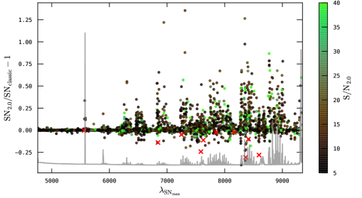
Figure 2: Comparison between of the SNs obtained with the improved filter, $\mathrm{SN}_{2.0}$ (Eq. 27), to those obtained with the classic filter, $\mathrm{SN}_{\mathrm{classic}}$ (Eq. 19), for all catalogued emission lines of the MUSE-Wide data release by Urrutia . (2019). The relative difference of $\mathrm{SN}_{2.0}$ with respect to $\mathrm{SN}_{\mathrm{classic}}$ is shown as a function of peak detection wavelength $\lambda_{\mathrm{SN_{\mathrm{peak}}}}$, and the absolute $\mathrm{SN}_{2.0}$ is colour coded as indicated by the colourbar (detections with $\mathrm{SN}_{2.0}>40$ are not assigned to a different colour than $\mathrm{SN}_{2.0}=40$ detections). The 10 emission lines for which $\mathrm{SN}_{2.0}$ is below the detection threshold of the original catalogue are marked by red crosses. An arbitrarily scaled variance spectrum is plotted as a grey line to indicate the spectral variation of the telluric background.

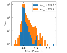
Figure 3: Stacked histogram (bin width = 0.05) of the relative differences of $\mathrm{SN}_{2.0}$ with respect to $\mathrm{SN}_{\mathrm{classic}}$ (cf. Fig. 2); emission lines at $\lambda_{\mathrm{SN_{\mathrm{peak}}}}\leq 7000$ Å are counted in blue, those at $\lambda_{\mathrm{SN_{\mathrm{peak}}}}7000$ Å are counted in orange.

We verified the expected improvement of detection significances with the method presented in Sect. 2.3 by a reanalysis of the publicly available data of MUSE-Wide survey (Urrutia . 2019). To this aim we reprocessed all released data cuboids in the same way as in the Urrutia . study, i.e., we used the template parameters provided in Table 2 of Urrutia . (2019), but now with the LSDCat2.0 routines. For each detected emission line we then compared the peak SN values between the original Ansatz (Sect. 2.2) and the improved Ansatz (Sect. 2.3) for all 3057 emission lines in the Urrutia . catalogue. The result of this exercise is presented in Figure 2, where we show for each catalogued detection the relative difference between the new and the old method, $\mathrm{SN}_{2.0}/\mathrm{SN}_{\mathrm{classic}}-1$, as a function of detection wavelength. Here $\mathrm{SN}_{2.0}$ refers to the peak values from Eq. (27), while $\mathrm{SN}_{\mathrm{classic}}$ refers to the peak values according to Eq. (19). We also inset an arbitrarily scaled effective variance spectrum into Figure 2 to illustrate the position and amplitude of the air-glow lines in the MUSE spectral range.

As can be seen from Figure 2, the improved Ansatz indeed boosts the SN of many detected emission lines especially in the forest of air glow lines. The overall improvement also becomes apparent in the histogram of relative SN differences shown in Figure 3. There we also separated the counts in each bin by their spectral position in the data cuboid, and again it can be seen how, especially in the red part of the spectrum, a significant number of sources experiences a boost in their detection significances. In numbers: 1892 detections have $\mathrm{SN}_{2.0}>\mathrm{SN}_{\mathrm{classic}}$, whereas for 1165 lines $\mathrm{SN}_{2.0}<\mathrm{SN}_{\mathrm{classic}}$. However, for the vast majority of detections where the improved algorithm provides a lower SN, the difference is marginal, whereas the boost for the former can be substantial. For example, while only 99 detections have $\mathrm{SN}_{2.0}<0.95\times\mathrm{SN}_{\mathrm{classic}}$, 722 show $\mathrm{SN}_{2.0}>1.05\times\mathrm{SN}_{\mathrm{classic}}$.

Nevertheless, we also find in this comparison that ten emission lines show a peak value that is marginally lower than the original detection threshold. All these catalogued lines are overlapping with air-glow lines, one even with the extremely strong [O i] $\lambda 5577$ line. For those lines the $\mathrm{SN}_{\mathrm{classic}}$ value got artificially boosted due to a strong positive noise contribution that gets adequately suppressed in the new formalism. Eight of those ten lines are secondary lines of emission line galaxies that have been detected in other, stronger, lines, i.e., these galaxies are not lost from the catalogue. The remaining two detections were supposed Ly$\alpha$ emitters, but these low SN detections were assigned also with the lowest confidence (i.e., $\approx$50% probability of being false detections according to Urrutia . 2019). Thus, our new algorithm does not remove significant detections from the previous catalogue, but significantly improves the detection significances of emission lines that are overlapping with air-glow lines. Hence, this little experiment verifies indeed that the new algorithm performs as expected.

We limited ourselves here to only check emission lines that were already catalogued. Nevertheless, because of the overall improvement of low-SN detections within the forest of the OH-bands we foresee that the LSDCat2.0 algorithm also uncovers new lines in those spectral regions. However, identifying and classifying new detections still requires manual inspection and verification by a team of experts (see Inami . 2017 and Urrutia . 2019 for descriptions of this process). Such a complete reanalysis of the MUSE-Wide dataset, clearly beyond the scope of the present work, may be desired for subsequent data MUSE-Wide releases.

3 The selection function of the 3D matched filter

A selection function, $f_{C}$ (sometimes also referred to as completeness function, e.g., in Caditz 2016), encodes the probability that a source with given attributes will enter our catalogue. Selection functions are needed whenever we want to construct a model of reality given the catalogue data (see Rix . 2021). Relevant applications in the context of surveys for emission line objects with IFS are, e.g., galaxy luminosity functions or modelling the galaxy power spectrum via correlation analysis (e.g., Blanc . 2011; Herenz . 2019; Herrero Alonso . 2021; Zhang . 2021). In terms of emission line source detection in IFS data cuboids the most important parameters are the wavelength, $\lambda$, of the detection and the flux of the emission line, $F_{\mathrm{line}}$.

Processing the flux data cuboids with a 3D matched filter (Eq. 15 or, more specifically, Eq. 27), can be understood as a linear mapping of $F_{\mathrm{line}}$ to SN space: $SN\propto F_{\mathrm{line}}$ (we recall from Sect. 2.1 that $\mathcal{T}^{x,y,z}$ can be understood as the maximised SN for a emission line at position $x,y,z$ in the data cuboid). The proportionality factor depends on the noise properties encountered at the spatial ($x,y$) and spectral ($\lambda$ or $z$) position of the emission line source in the data cuboid and on the level of congruence between template $\bm{S}$ and actual emission line source. For the construction of the filter we explicitly assumed in Sect. 2.3 that the noise properties are not an implicit function of position ($x,y$) and that the effect of varying depth over the field of view can be accounted for by rescaling. Moreover, because of the randomness of the noise, the value of SN is stochastic and thus we can abbreviate the mapping as

$$E[SN_{\mathrm{\lambda}}]=C(\lambda)\times F_{\mathrm{line}}\;\text{,}$$ (28)

where $E[SN_{\mathrm{\lambda}}]$ denotes the expectation value of $SN_{\mathrm{\lambda}}$ and $C(\lambda)$ is in units of inverse flux. We also assumed that the noise is normally distributed and uncorrelated, thus the distribution of $SN_{\mathrm{\lambda}}$ for a given $F_{\mathrm{line}}$, $g(SN_{\lambda}|F_{\mathrm{line}})$, is also normal and with variance $V[SN_{\mathrm{\lambda}}]=1$, i.e.,

$$g(SN_{\lambda}|F_{\mathrm{line}})=\frac{1}{\sqrt{2}}\exp\left(-\frac{(SN_{\lambda}-C(\lambda)F_{\mathrm{line}})^{2}}{2}\right)\;\mathrm{.}$$ (29)

Now the selection function, $f_{C}(F_{\mathrm{line}},\lambda|\mathrm{SN}_{\mathrm{thresh}})\in[0,1]$, encodes the cumulative probability that $F_{\mathrm{line}}$ will result in $SN_{\mathrm{\lambda}}(F_{\mathrm{line}})>\mathrm{SN}_{\mathrm{thresh}}$, i.e.,

$$f_{C}(F_{\mathrm{line}},\lambda|\mathrm{SN}_{\mathrm{thresh}})=\int_{\mathrm{SN}_{\mathrm{thresh}}}^{\infty}g(SN_{\lambda}|F_{\mathrm{line}})\,\mathrm{d}(SN_{\mathrm{\lambda}})$$ (30)

for a given a detection threshold $\mathrm{SN}_{\mathrm{thresh}}$. Using the error-function,

$$\operatorname{erf}(x)=\frac{2}{\sqrt{\pi}}\int_{0}^{x}e^{-t^{2}}\,\mathrm{d}t=1-\frac{2}{\sqrt{\pi}}\int_{x}^{\infty}e^{-t^{2}}\,\mathrm{d}t\;\text{,}$$ (31)

we can express the selection function in Eq. (30) as

$$f_{C}(F_{\mathrm{line}},\lambda|\mathrm{SN}_{\mathrm{thresh}})=\\ =\frac{1}{2}\left[1+\operatorname{erf}\left(\frac{C(\lambda)\times F_{\mathrm{line}}-\mathrm{SN}_{\mathrm{thresh}}}{\sqrt{2}}\right)\right]\;\text{.}$$ (32)

Due to the symmetry of the normal distribution, Eq. (32) is also symmetric around $F_{\mathrm{line}}$, and this flux thus equates with the 50 % completeness limit which we now denote $F_{50}$, i.e., $f_{C}(F_{50},\lambda|\mathrm{SN}_{\mathrm{thresh}})\equiv 0.5$ and

$$F_{50}=\frac{\mathrm{SN}_{\mathrm{thresh}}}{C(\lambda)}\;\text{.}$$ (33)

As can be seen, the selection function is completely determined if the proportionality factor $C(\lambda)$ is known and in the remainder of this section we have to deal with calculations of $C(\lambda)$.

3.1 The idealised selection function

We define the idealised selection function as the selection function for an emission line source in the data cuboid that is perfectly matched by the source template $\bm{S}$ (Eq. 17 and Eq. 18). For the calculation of $C(\lambda)$ we calculate the response of the filter for such a source at some position $x^{\prime},y^{\prime},z^{\prime}$ in the data cuboid $\bm{F}$:

$$F_{x,y,z}=A\cdot S_{x-x^{\prime},y-y^{\prime}}^{\mathrm{spat}}S^{\mathrm{spec}}_{z-z^{\prime}}+n_{x,y,z}\;\text{,}$$ (34)

where $A$ is the amplitude at which the normalised source profile and $n_{x,y,z}$ describes a source-free noise cuboid. Then the matched filter of Eq. (27) with the template according to Eq. (25) and Eq. (26) has the expectation value

$$E_{\mathcal{I}}\left[\mathcal{T}^{(x^{\prime},y^{\prime},z^{\prime})}\right]=A\cdot\sqrt{\sum_{ij}\left(S_{ij}^{\{z^{\prime}\}}\right)^{2}}\cdot\sqrt{\sum_{k}\frac{\left(S_{k}^{\{z^{\prime}\}}\right)^{2}}{\sigma_{z^{\prime}-k}^{2}}}\;\text{,}$$ (35)

where we used $E[n_{x,y,z}]=0$. In anticipation of the discussion in Sect. 3.3 below we wrote $E_{\mathcal{I}}$ in Eq. (35) to signify that this is the expectation value for the idealised scenario.

A voxel in the flux data cuboid $F_{x,y,z}$ is assumed to encode flux density. For example, MUSE data reduction pipeline provides fluxes in erg s^-1cm^-2Å. The amplitude A in Eq. (34) then relates to the emission line flux $F_{\mathrm{line}}$ in erg s^-1cm^-2 via

$$A=F_{\mathrm{line}}/\Delta\lambda\;\text{,}$$ (36)

where $\Delta\lambda$ is the native wavelength sampling of the data cuboid (default $\Delta\lambda=1.25$ Å for MUSE). The wavelength $\lambda$ relates linearly to the spectral coordinate $z$ (cf. Eq. 73 in A) and we abbreviate it by $\lambda[z]$. We now equate Eq. (28) with Eq. (35) to find

$$C_{\mathcal{I}}(\lambda[z])=\frac{1}{\Delta\lambda}\cdot\sqrt{\sum_{ij}\left(S_{ij}^{\{z\}}\right)^{2}}\cdot\sqrt{\sum_{k}\frac{\left(S_{k}^{\{z\}}\right)^{2}}{\sigma_{z-k}^{2}}}\;\text{,}$$ (37)

where again the subscript $\mathcal{I}$ signifies that this is the proportionality constant for the idealised selection function.

Equation (32) with $C(\lambda[z])$ from Eq. (37) provides an expression for the idealised selection function for the line search with some template $\bm{S}$ (Eq. 17) given an effective variance spectrum $\sigma^{2}_{z}$.

3.2 Verification of the analytical expression for the idealised selection function

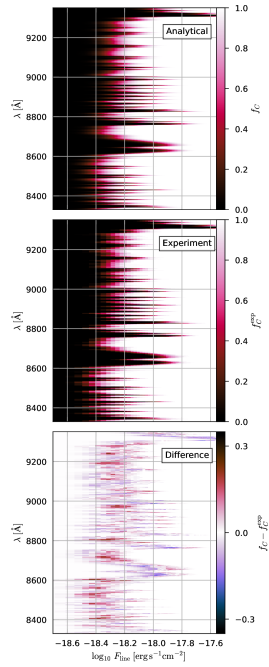
Figure 4: Comparison between the idealised selection function according to Eq. (32) with $C(\lambda)$ from Eq. (37) ($f_{C}$, top panel) to the idealised selection function from a source insertion and recovery experiment ($f_{C}^{\mathrm{exp}}$, centre panel) for a $z>6$ LAE search with LSDCat2.0 in the MXDF (Bacon . 2022) using the template given in Table 1 and a detection threshold of $SN_{\mathrm{thresh}}=6.41$. The bottom panel shows the difference $f_{C}-f_{C}^{\mathrm{exp}}$.

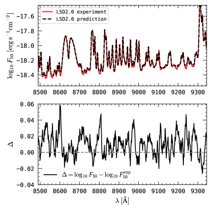
Figure 5: Analytical 50% completeness estimate in comparison to the 50% completeness achieved in a source insertion and recovery experiment, $F_{50}^{\mathrm{exp}}$, for the LSDCat2.0 line search at $\lambda>8500$ Å in the MXDF with $SN_{\mathrm{thresh}}=6.41$ under the assumption of idealised sources described by the 3D template in Table 1. The top panel displays both the analytical $\log_{10}F_{50}$ (Eq. 33 with $C(\lambda)$ from Eq. 37; dashed black line) and the $\log_{10}F_{50}^{\mathrm{exp}}$ from the numerical experiment (red line), whereas the bottom panel displays the difference $\Delta=\log_{10}F_{50}-\log_{10}F_{50}^{\mathrm{exp}}$.

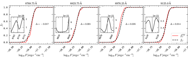
Figure 6: Analytical completeness curves (dashed black lines; Eq. 32 with $C(\lambda)$ from Eq. 37) in comparison to the completeness curves from a source insertion and recovery experiment (red lines) for the LSDCat2.0 line search in the MXDF (see text and captions to Figures 4 and 5 for details) at four representative wavelength layers. In each panel we print the difference $\Delta=\log_{10}F_{50}^{\mathrm{ana}}-\log_{10}F_{50}^{\mathrm{exp}}$ (cf. Fig. 5) and we inset a zoom-in of the extracted average noise spectrum ($\sqrt{\sigma^{2}_{z}}$ in erg s^-1cm^-2Å^-1) around the layers of interest.

We performed a source insertion and recovery experiment to check whether Eq. (32) with $C(\lambda)$ from Eq. (37) can indeed predict the idealised selection function of the algorithm. For this experiment we used the recently released data cuboid of the MUSE eXtreme Deep Field (MXDF) by Bacon . (2022). This dataset is the deepest blank field ever obtained with MUSE ($t_{\mathrm{exp}}=141$ h). In order to reduce potential systematics, this programme used a non-standard observing strategy where each subsequent observing block was rotated by a few degrees. The result is that the final combined field of view within the data cuboid is circular. As groundwork for future population studies of unprecedented faint Ly$\alpha$ emitters in this dataset we constructed an emission line emitter catalogue with LSDCat. For reference we list the template parameters that were used in this search in C (Table 1). The detection threshold for this search is $SN_{\mathrm{thresh}}=6.41$. This value was found to be the “point of diminishing returns” from the ratio of the number of detections in the normal datacube to the number of detections in the negated datacube (see Sect. 4.5 in HW17). For the demonstration here we only consider the extreme red of the MUSE spectral range, where the density and amplitude of the telluric background emission lines is highest.

For the recovery experiment we implanted emission line sources into the MXDF that are exactly described by this template. We used a regular grid of 70 insertion positions and we considered only the central region of $>140$ h depth (see Fig. 3 in Bacon . 2022). The distance between neighbouring sources was 6^′′. At each wavelength layer $\lambda[z]$ we then inserted the artificial line sources with fluxes from $\log_{10}F_{\mathrm{line}}^{\mathrm{ins}}$[erg s^-1cm^-2]$=-18.6$ to $\log_{10}F_{\mathrm{line}}^{\mathrm{ins}}$[erg s^-1cm^-2]$=-17.1$ at an increment of $3\times 10^{-20}$erg s^-1cm^-2; in each insertion experiment all sources have the same flux. After each insertion we ran the full source detection chain that was used for the construction of the catalogue, i.e., we subtracted a running median to remove continuum emission and we ran the 3D matched-filter with the template given in Table 1. We then counted the number of recovered lines above $SN_{\mathrm{thresh}}$ which, divided by the number of inserted sources, provides us with the experimentally determined completeness $f_{C}^{\mathrm{exp.}}(F_{\mathrm{line}}^{\mathrm{ins}},\lambda[z])$ for each ($F_{\mathrm{line}}^{\mathrm{ins}},\lambda[z]$)-pair. We excluded detections of real sources in our tally by excluding insertion positions that overlapped with detections of real emission line sources in the original search, i.e., in some layers the denominator of inserted sources was less than 70 for the calculation of $f_{C}^{\mathrm{exp.}}(F_{\mathrm{line}}^{\mathrm{ins}},\lambda[z])$.

In Figure 4 we show a comparison between the analytic prediction for the idealised case, i.e., $f_{C}(\lambda,F_{\mathrm{line}}|SN_{\mathrm{thresh}}=6.41)$ according to Eq. (32) with $C(\lambda)$ from Eq. (37) for the template parameters given in Table 1, and the experimentally determined selection function, $f_{C}^{\mathrm{exp}}$, from the above described insertion and recovery procedure. To compute the analytic prediction we evaluated Eq. (37) we calculated the effective variance spectrum (Eq. 23) as the median in each layer of the variance cube in the central $141$ h deep region. The visual comparison between the analytical prediction (top panel of Figure 4) with the experimental result (middle panel of Figure 4) does not reveal large discrepancies. Only the sampling in $\log_{10}F$ of the numerical experiment becomes apparent as pixelated structure in the middle panel. Obviously, the analytic prediction can be evaluated on a much finer flux grid than what would be feasible for an insertion and recovery experiment. The impression of congruity between prediction and experiment is verified in the bottom panel of Fig. 4, where we show the difference between the $f_{C}$ and $f_{C}^{\mathrm{exp}}$. Only very few $(F_{\mathrm{line}},\lambda)$-bins show a difference greater than 20%, and generally the experimental and analytical curves are close to each other.

The congruence between prediction and experiment can also be appreciated in Figure 5, where we compare the analytic 50% completeness (Eq. 33) to the 50% completeness from the experiment. The latter was calculated via linear interpolation using the two flux insertion values for which $f_{C}^{\mathrm{exp}}$ had the smallest absolute difference to $0.5$. Again, both curves are nearly identical, with the average $\Delta=\log_{10}F_{50}-\log_{10}F_{50}^{\mathrm{exp}}$ being $0.01$. Inspecting Figures 4 and 5 in detail reveals that the experiment results in slightly deeper flux limits, but the discrepancies are marginal and dwarfed in comparison to the uncertainties on the selection function due to mismatches between filter template and real sources (see Sect. 3.3 below). Importantly, the fluctuations on $\Delta$ appear random and do not correlate with features in the sky background.

Lastly, we compare in Figure 6 the analytic $f_{C}(F_{\mathrm{line}},\lambda)$ curves with their experimental counterparts for four different wavelength layers. These layers are chosen to be representative for the typical situations in the background noise spectrum. The first and the third panel (from the left) demonstrate the selection function for wavelength layers that are in the wings of a [OH]-line, whereas the second panel shows a layer were the surrounding noise spectrum is not varying strongly. The fourth panel shows the $f_{C}$ curve for a layer where the background noise is lower, but with sharp spikes rising in the redward and blueward layers; this situation is akin to the example discussed in Sect. 2.2 (Figure 1). Again, all experimental curves show an good level of agreement with the analytic predictions.

3.3 Towards a realistic selection function

The idealised situation analysed in the previous section, where astronomical sources match exactly the template used for the filtering, is never encountered in the reality of blind surveys. Each real world emission line source can have different spectral and spatial profiles. A motivated strategy for the line search is to opt for a template that maximises the SN for a large fraction of the desired sources in the final sample. This may be achieved iteratively by varying the template parameters and checking the SN response of sources found in a previous iteration or even a previous survey in the same field (see Fig. 7 of HW17). We will introduce a metric to quantify the loss in SN with respect to the source matching filter below (Eq. 47). If this loss is undesirable high for a large fraction of the targeted population, one might even consider to construct a catalogue from multiple filter templates. In this case, additional bookkeeping is required to track which template resulted in a source entering the catalogue, and multiple entries for an individual sources recovered with different templates need to be weeded out. We will not consider this case further here. The aim of this section is rather to provide ideas towards answering question: “What is the realistic selection function for a given source population in the catalogue that results from the search with a template $\bm{S}$?”. We understand as “source population” here a class of emission line objects, e.g., high-redshift LAEs, whose spatial and spectral properties are understood in a statistical sense.

3.3.1 Formalism for source-template mismatches

In order to find a realistic selection function as defined above we first have to analyse what happens to $f_{C}$ for a single type of source that is that is not matched by the search template. To this aim we have to calculate the response of the 3D filtering operation in Eq. (27) to the non-template matching source. We start by defining the voxels of the non-template matching source profile, $\bm{\widetilde{S}}$, where the spatial and spectral components are independent of each other

$$\widetilde{S}_{x,y,z}=\widetilde{S}_{xy}^{\mathrm{spat}}\widetilde{S}_{z}^{\mathrm{spec}}\;\text{,}$$ (38)

where $\widetilde{S}_{ij}^{\mathrm{spat}}\neq{S}_{ij}^{\mathrm{spat}}$ and $\widetilde{S}_{k}^{\mathrm{spec}}\neq{S}_{k}^{\mathrm{spec}}$ for ${S}_{ij}^{\mathrm{spat}}$ and ${S}_{k}^{\mathrm{spec}}$ from Eq. (17). Moreover, $\bm{S}$ is normalised: $\sum_{ijk}\widetilde{S}_{ijk}\equiv\sum_{ij}\widetilde{S}_{ij}^{\mathrm{spat}}\equiv\sum_{k}\widetilde{S}_{k}^{\mathrm{spec}}\equiv 1$. We now insert this source at position $x^{\prime},y^{\prime},z^{\prime}$ into a data cuboid that contains otherwise only noise. In the spirit of Eq. (34) we write

$$F_{x,y,z}=\xi\cdot A\cdot\widetilde{S}_{x-x^{\prime},y-y^{\prime}}^{\mathrm{spat}}\widetilde{S}_{z-z^{\prime}}^{\mathrm{spec}}+n_{x,y,z}\;\text{.}$$ (39)

with the amplitude $A$ as defined in Eq. (36). Here we introduced the factor $\xi$ that will provide us with the required rescaling of the line flux, $\xi\cdot F_{\mathrm{line}}$, in order to make the expectation value of the filter in Eq. (27) at position $x^{\prime},y^{\prime},z^{\prime}$ for the source given in Eq. (39),

$$E_{\xi}\left[\mathcal{T}^{(x^{\prime},y^{\prime},z^{\prime})}\right]=\frac{\xi\cdot A^{2}}{E_{\mathcal{I}}\left[\mathcal{T}^{(x^{\prime},y^{\prime},z^{\prime})}\right]}\cdot\sum_{k}\frac{S_{k}^{\{z^{\prime}\}}\widetilde{S}_{k}^{\mathrm{spec}}}{\sigma^{2}_{z^{\prime}-k}}\cdot\sum_{ij}S_{ij}^{\{z^{\prime}\}}\widetilde{S}_{ij}^{\mathrm{spat}}\;\text{,}$$ (40)

identical to the expectation value $E_{\mathcal{I}}[\mathcal{T}^{(x^{\prime},y^{\prime},z^{\prime})}]$ from Eq. (35). Formally, we thus require

$$E_{\xi}[\mathcal{T}^{(x^{\prime},y^{\prime},z^{\prime})}]\stackrel{{\scriptstyle!}}{{=}}E_{\mathcal{I}}[\mathcal{T}^{(x^{\prime},y^{\prime},z^{\prime})}]\;\text{,}$$ (41)

and evaluating this condition results in

$$\xi(\lambda[z])=\cfrac{\sum_{n}\cfrac{\left(S_{n}^{\{z\}}\right)^{2}}{\sigma_{z-n}^{2}}\cdot\sum_{ij}\left(S_{ij}\right)^{2}}{\sum_{n}\cfrac{S_{n}^{\{z\}}\widetilde{S}^{\mathrm{spec}}_{n}}{\sigma_{z-n}^{2}}\cdot\sum_{ij}S_{ij}\widetilde{S}_{ij}^{\mathrm{spat}}}$$ (42)

as expression for the required flux rescaling factor. Moreover, denoting with $C_{\widetilde{S}}$ the proportionality factor in units of inverse flux (Eq. 28) that needs to be used in the selection function (Eq. 32) or for the 50%-completeness limit (Eq. 33), and noting that Eq. (42) can also be expressed as

$$\xi=\frac{E_{\xi}^{2}}{A^{2}}\Bigg{/}\frac{E_{\xi}E_{\mathcal{I}}}{A^{2}}=\frac{E_{\mathcal{I}}}{E_{\xi}}\;\text{,}$$ (43)

were we dropped the arguments of the expectation values and $\xi$, we also recover

$$\xi(\lambda)=\frac{C_{\mathcal{I}}(\lambda)}{C_{\widetilde{S}}(\lambda)}\quad\text{or}\quad C_{\widetilde{S}}(\lambda)=\frac{C_{\mathcal{I}}(\lambda)}{\xi(\lambda)}\;\text{.}$$ (44)

The rescaling of the flux axis of the ideal selection function with $\xi$ from Eq. (42) or the rescaling of the proportionality factor $C_{\mathcal{I}}(\lambda)$ from Eq. (37) with $\xi^{-1}$ (Eq. 44) are of practical relevance for the calculation of a non-template matching source’s selection function.

It is, moreover, also of interest to quantify the relative loss in SN at a fixed $F_{\mathrm{line}}$ (i.e., $\xi\equiv 1$) due to the source-template mismatch with respect to the SN that would be obtained for a filter that is perfectly matched to the source. In analogy to Eq. (35) we can write the optimal expectation value for the SN of the source in Eq. (39) as

$$E_{\mathcal{\widetilde{S}}}\left[\mathcal{T}^{(x^{\prime},y^{\prime},z^{\prime})}\right]=A\cdot\sqrt{\sum_{ij}\left(\widetilde{S}_{ij}\right)^{2}}\cdot\sqrt{\sum_{k}\frac{\left(\widetilde{S}_{k}\right)^{2}}{\sigma_{z^{\prime}-k}^{2}}}\;\text{.}$$ (45)

Denoting with $E_{\xi=1}\left[\mathcal{T}^{(x^{\prime},y^{\prime},z^{\prime})}\right]$ the expectation value from Eq. (40) for $\xi=1$ the loss in SN relative to the matched filter for $\bm{\widetilde{S}}$ is then given by the ratio

$$\zeta(\lambda[z^{\prime}])=\frac{E_{\xi=1}\left[\mathcal{T}^{(x^{\prime},y^{\prime},z^{\prime})}\right]}{E_{\mathcal{\widetilde{S}}}\left[\mathcal{T}^{(x^{\prime},y^{\prime},z^{\prime})}\right]}$$ (46)

$$=\cfrac{\sum_{n}\frac{S_{n}^{\{z^{\prime}\}}\widetilde{S}^{\mathrm{spec}}_{n}}{\sigma_{z^{\prime}-n}^{2}}\cdot\sum_{ij}S_{ij}\widetilde{S}_{ij}^{\mathrm{spat}}}{\sqrt{\sum_{n}\frac{\left(S_{n}^{\{z^{\prime}\}}\right)^{2}}{\sigma_{z^{\prime}-n}^{2}}}\sqrt{\sum_{ij}\left(S_{ij}^{\{z^{\prime}\}}\right)^{2}}\sqrt{\sum_{n}\frac{\left(\widetilde{S}_{n}\right)^{2}}{\sigma_{z^{\prime}-n}^{2}}}\sqrt{\sum_{ij}\left(\widetilde{S}_{ij}\right)^{2}}}\;\text{.}$$ (47)

This quantity provides a figure of merit to judge the quality of the applied template for a particular source.

Equation (42) and Eq. (47) have to be evaluated numerically for any source profile described by Eq. (38) and any template profile that is described by Eq. (18).

3.3.2 Source-template mismatches in the spatial and spectral domain

In principle, we are not restricted by the stated requirement that the spectral and spatial component of the coveted source profile are independent of each other (Eq. 38). The expectation values $E_{\xi}$ in Eq. (40) and $E_{\mathcal{\widetilde{S}}}$ in Eq. (45) could be calculated numerically for an arbitrary 3D profile, $\bm{\mathcal{\widetilde{S}}}$, and from those expectation values then $\xi$ (Eq. 43) and $\zeta$ follow (Eq. 46). However, the separation allows us especially to analyse the expected effects of source template mismatches in the spectral and spatial domain separately. This also allows us to develop intuition for the magnitude of the flux rescaling of the selection function and the corresponding expected loss in SN for realistic profiles (see also Sect. 3.3.3).

We first consider the case where only the spatial part of the source profile differs from the template, but where the spectral part is a perfect match ($\widetilde{S}_{ij}^{\mathrm{spat}}\neq{S}_{ij}^{\mathrm{spat}}$, but $\widetilde{S}_{k}^{\mathrm{spec}}\equiv{S}_{k}^{\mathrm{spec}}$). Then Eq. (42) reduces to

$$\xi(\lambda[z])=\frac{\sum_{ij}\left(S_{ij}^{\{z\}}\right)^{2}}{\sum_{ij}S_{ij}^{\{z\}}\widetilde{S}_{ij}^{\mathrm{spat}}}\;\text{,}$$ (48)

and Eq. (47) becomes

$$\zeta(\lambda[z])=\frac{\sum_{ij}S_{ij}^{\{z\}}\widetilde{S}_{ij}^{\mathrm{spat}}}{\sqrt{\sum_{ij}\left(S_{ij}^{\{z\}}\right)^{2}}\sqrt{\sum_{ij}\left(\widetilde{S}_{ij}^{\mathrm{spat}}\right)^{2}}}\;\text{.}$$ (49)

As a direct consequence of the spatially invariant variance (Eq. 23) the pure spatial mismatch of template and source profile leads to rescaling of the selection function (Eq. 48) or loss in SN (Eq. 49) that is independent of the variance. Moreover, Eq. (48) and Eq. (49) also describe the rescaling of the limiting flux and the loss in S/N due to template mismatch for the detection of background limited sources via matched filtering in imaging data if the variance can be assumed to be constant for every pixel.

We can go one step further and provide analytical expressions for Eq. (48) and Eq. (49) for the case where both the source and the template are 2D Gaussian profiles that differ in their dispersions. Neglecting sampling effects, i.e. we assume that the pixel size is significantly smaller than the dispersions of the profiles, allows us to replace the summations by integrals. Thus, writing $\sigma_{\mathrm{T}}$ for the 2D template dispersion and $\sigma_{\mathrm{S}}$ the 2D source dispersion we find

$$\sum_{ij}\left(S_{ij}\right)^{2} \simeq\frac{1}{4\pi^{2}\sigma_{\mathrm{T}}^{4}}\int_{-\infty}^{+\infty}\int_{-\infty}^{+\infty}\exp\left(-\frac{x^{2}+y^{2}}{\sigma_{\mathrm{T}}^{2}}\right)\,\mathrm{d}x\mathrm{d}y$$

$$=\frac{1}{4\pi\sigma_{\mathrm{T}}^{2}}$$ (50)

and

$$\sum_{ij}S_{ij}\widetilde{S}_{ij}^{\mathrm{spat}}\simeq\\ \simeq\frac{1}{4\pi^{2}\sigma_{\mathrm{T}}^{2}\sigma_{\mathrm{S}}^{2}}\int_{-\infty}^{+\infty}\int_{-\infty}^{+\infty}\exp\left(-\frac{1}{2}\frac{\sigma_{\mathrm{T}}^{2}+\sigma_{\mathrm{S}}^{2}}{\sigma_{\mathrm{S}}^{2}\sigma_{\mathrm{T}}^{2}}(x^{2}+y^{2})\right)\,\mathrm{d}x\mathrm{d}y\\ \quad\;\,=\frac{1}{2\pi(\sigma_{\mathrm{S}}^{2}+\sigma_{\mathrm{T}}^{2})}\;\text{.}\hfill$$ (51)

Then, inserting Eq. (3.3.2) and Eq. (51) into Eq. (48), and introducing the 2D Gaussian template mismatch factor,

$$\chi_{\mathrm{2D}}=\frac{\sigma_{\mathrm{S}}}{\sigma_{\mathrm{T}}}\;\text{,}$$ (52)

we obtain

$$\xi=\frac{\sigma_{\mathrm{S}}^{2}+\sigma_{\mathrm{T}}^{2}}{2\sigma_{\mathrm{T}}^{2}}=\frac{1+\chi_{\mathrm{2D}}^{2}}{2}$$ (53)

as the required flux rescaling factor of the non-template matching 2D Gaussian to reach the same SN as a template matching 2D Gaussian. Moreover, using the results from Eq. (3.3.2) and Eq. (51) in Eq. (49) leads to

$$\zeta=\frac{2\sigma_{\mathrm{T}}\sigma_{\mathrm{S}}}{\sigma_{\mathrm{T}}^{2}+\sigma_{\mathrm{S}}^{2}}=\frac{2\chi_{\mathrm{2D}}}{1+\chi_{\mathrm{2D}}^{2}}$$ (54)

as the loss in SN at fixed flux. Equation (54) was derived in a slightly different way by Zackay  Ofek (2017) in the context of source detection in co-added images (their Appendix D).

Considering the case where only the spectral part of the source profile differs from that of the template and where the spatial part is perfectly matched ($\widetilde{S}_{k}^{\mathrm{spec}}\neq{S}_{k}^{\mathrm{spec}}$ and $\widetilde{S}_{ij}^{\mathrm{spat}}\equiv{S}_{ij}^{\mathrm{spat}}$) we find from Eq. (42)

$$\xi(\lambda[z])=\sum_{n}\cfrac{\left(s_{n}^{\{z\}}\right)^{2}}{\sigma_{z-n}^{2}}\Bigg{/}\sum_{n}\cfrac{S_{n}^{\{z\}}\widetilde{S}_{n}^{\mathrm{spec}}}{\sigma_{z-n}^{2}}\;\text{,}$$ (55)

and Eq. (47) reduces to

$$\zeta(\lambda[z])=\cfrac{\sum_{n}\frac{S_{n}^{\{z\}}\widetilde{S}^{\mathrm{spec}}_{n}}{\sigma_{z^{\prime}-n}^{2}}}{\sqrt{\sum_{n}\frac{\left(S_{n}^{\{z\}}\right)^{2}}{\sigma_{z-n}^{2}}}\sqrt{\sum_{n}\frac{\left(\widetilde{S}_{n}\right)^{2}}{\sigma_{z-n}^{2}}}}\;\text{.}$$ (56)

The rescaling of the flux and loss in SN for purely spectral template mismatches in Eq. (55) and Eq. (56), respectively, depend on wavelength due to the spectrally varying variances.

To compute reference values for $\xi$ and $\zeta$ for 1D source-template mismatches we assume for a moment that the variances are not varying over the extent of the filters and the source, since this allows for analytical estimate for 1D Gaussians (Eq. 72) of different dispersions. The calculations are completely analogous to the the 2D case in Eq. (3.3.2) and Eq. (51). We find

$$\xi_{\mathrm{ref}}=\sqrt{\frac{\sigma_{\mathrm{T,1D}}^{2}+\sigma_{\mathrm{S,1D}}^{2}}{2\sigma_{\mathrm{T,1D}}^{2}}}=\sqrt{\frac{1+\chi_{\mathrm{1D}}^{2}}{2}}$$ (57)

and

$$\zeta_{\mathrm{ref}}=\sqrt{\frac{2\sigma_{\mathrm{T,1D}}^{2}\sigma_{\mathrm{S,2D}}^{2}}{\sigma_{\mathrm{T,1D}}^{2}+\sigma_{\mathrm{S,1D}}^{2}}}=\sqrt{\frac{2\chi_{\mathrm{1D}}}{1+\chi_{\mathrm{1D}}^{2}}}$$ (58)

where $\sigma_{\mathrm{T,1D}}$ and $\sigma_{\mathrm{S,1D}}$ are the dispersions of the template and source 1D Gaussian, respectively, and

$$\chi_{\mathrm{1D}}=\frac{\sigma_{\mathrm{S,1D}}}{\sigma_{\mathrm{T,1D}}}$$ (59)

is the 1D Gaussian template mismatch factor. The subscript “ref” in Eq. (57) and Eq. (58) explicitly indicates that these values are reference values that are derived in the absence of spectrally varying variances.

We see that the flux rescaling (Eq. 57) and SN loss factor (Eq. 58) for the 1D Gaussian mismatch vary as a square root of the expressions that were derived for the 2D Gaussian mismatch (Eq. 53 and Eq. 54). Thus, in the absence of spectrally varying variances the selection function appears more robust against source-template mismatches in the spectral domain than against source-template mismatches in the spatial domain. This argument was already stated in HW17, but without the formal justification provided here.

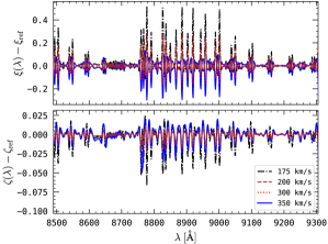
Figure 7: Illustration of the effects due to source-template mismatches in the spectral domain for 1D Gaussians (Eq. 72) that are not matched in width by the 1D Gaussian search template. We show results for $v_{\mathrm{FWHM}}^{\mathrm{template}}=250$ km s^-1 and, as indicated in the legend, $v_{\mathrm{FWHM}}^{\mathrm{source}}=\{175,200,300,350\}$ km s^-1. Top panel: Difference between the flux rescaling factor, $\xi(\lambda)$ from Eq. (55), and the reference rescaling factor, $\xi_{\mathrm{ref}}$ from Eq. (57), that would be needed in the absence of spectrally varying variances. Bottom panel: Difference between the loss in SN, $\zeta(\lambda)$ from Eq. (56), and the reference value, $\zeta_{\mathrm{ref}}$ from Eq. (58), that would follow in the absence of spectrally varying variances. For the evaluation of Eq. (55) and Eq. (56) we here again used the effective variance spectrum of the MXDF (see Sect. 3.2), thus similar results are expected for the typical telluric background in the red part of the optical spectral range.

Now it remains to be analysed how the mismatch between a 1D Gaussian filter and source in the spectral domain are affected by a spectrally rapidly varying background. To illustrate this, we compare in Figure 7 the difference between the calculated values for $\xi(\lambda)$ (Eq. 55) and $\zeta(\lambda)$ (Eq. 56) and the reference values $\xi_{\mathrm{ref}}$ (Eq. 57) and $\zeta_{\mathrm{ref}}$ (Eq. 58). We here analyse mismatches for $v_{\mathrm{FWHM}}^{\mathrm{template}}=250$ km s^-1 and $v_{\mathrm{FWHM}}^{\mathrm{source}}=\{175,200,300,350\}$ km s^-1, that is $\chi_{\mathrm{1D}}=\{0.7,0.8,1.2,1.4\}$ and hence $\xi_{\mathrm{ref}}=\{0.86,0.91,1.10,1.21\}$ and $\zeta_{\mathrm{ref}}=\{0.969,0.998,0.992,0.973\}$. We show the results of the calculations for the red part of the MUSE spectral range, where we have the highest density and amplitudes of the sky emission lines. Here we used again the effective variance spectrum of the MXDF (Sect. 3.2). This variance spectrum provides a good average of the sky-line amplitudes over large window in time at Cerro Paranal, hence the results shown in Figure 7 appear universal.

In the bottom panel of Figure 7 we find $\zeta(\lambda)<\zeta_{\mathrm{ref}}$ in the vicinity of sky lines, i.e. at fixed line flux the recovered SN is slightly lower than what is expected for a constant background. This is because the template does not correctly modulate the shot-noise from the sky lines with respect to the source profile. While the difference $\zeta(\lambda)-\zeta_{\mathrm{ref}}$ is small, it is of comparable amplitude as the reference value, $\zeta_{\mathrm{ref}}$, for the expected loss in SN. Of more practical relevance for the selection function is, nevertheless, the difference $\xi(\lambda)-\xi_{\mathrm{ref}}$. This difference is shown in the top panel of Figure 7. We find $\xi(\lambda)>\xi_{\mathrm{ref}}$ for $v_{\mathrm{FWHM}}^{\mathrm{source}}<v_{\mathrm{FWHM}}^{\mathrm{template}}$ in the vicinity of sky lines. This is because the filter weighs the increased background noise stronger in its wings compared to what would be appropriate given the source profile. The result is that a larger flux rescaling is required with respect to the reference value at stationary noise. On the other hand, we have $\xi(\lambda)<\xi_{\mathrm{ref}}$ in the vicinity of sky-lines for $v_{\mathrm{FWHM}}^{\mathrm{source}}>v_{\mathrm{FWHM}}^{\mathrm{template}}$. This is because the smaller width of filter template suppresses the variances in the wings stronger than needed, while the flux from the wings of the source profile does not contribute optimally to the signal. Hence, slightly less flux rescaling is needed in comparison to the reference value at stationary noise for templates that are smaller then the source profile.

In summary, we find that in the presence of a rapidly varying spectral background also spectral template mismatches need to be taken into account for a correct estimate of the selection function. Variations due to spatial template mismatches will only dominate the required rescaling of the selection function in the case of a slowly varying or constant background.

3.3.3 Examples for realistic source-template mismatches in LAE searches

We now analyse two more realistic source-template mismatches. The examples presented here appear of practical interest for emission line searches, and especially searches for LAEs, in deep wide-field IFS datacubes. As search template we use here the template that was used for the search of faint Ly$\alpha$ emitters in the MXDF (see C; Herenz et al., in prep.).

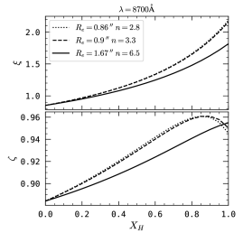
Figure 8: Rescaling ($\xi$, Eq. 48, top panel) and loss in SN ($\zeta$, Eq. 49, bottom panel) for average high-redshift LAE surface brightness profiles when recovered with the search template that was optimised for the recovery of known LAEs in the MXDF (Table 1). Equation (48) and Eq. (49) were evaluated for this plot at $\lambda=8700$ Å. The source surface brightness profiles are described PSF core + Sèrsic halo according to Eq. (61), where the parameters for the Sèrsic halo (Eq. 60) are from Wisotzki . (2018; their Extended Data Table 1) as indicated in the legend. The PSF component is modelled as a wavelength dependent Moffat (Eq. 70) according to Table 2.

Example 1: Moffat core + Sérsic halo profiles

The spatial distribution of Ly$\alpha$ emission from high-redshift LAEs can almost always be characterised by a spatially unresolved “point-like” core component and an extended halo component. The physical nature of the extended Ly$\alpha$ emission is not completely understood, but resonant scatterings of Ly$\alpha$ photons in neutral halo gas are thought to be a dominant mechanism (e.g., Steidel . 2011; Hayes . 2013; Wisotzki . 2016; Mas-Ribas  Dijkstra 2016; Leclercq . 2017; Lujan Niemeyer . 2022).

We here follow Wisotzki . (2018) who parameterised the average halo profile of these sources with a Sersic (1968) profile:

$$I_{H}(r)=I_{H}(0)\times\exp\left(-\left[\frac{r}{R_{e}}\right]^{1/n}\right)\;\text{.}$$ (60)

Here the parameters $R_{e}$ and $n$ define the characteristic radius and the kurtosis of the profile (Graham  Driver 2005). The observable profile of the “point-like + halo” model can then be written as

$$\widetilde{S}(r,\lambda)=I_{0}\cdot\mathrm{PSF}(r,\lambda)\star\left\{(1-X_{\mathrm{H}})\delta(r)+X_{\mathrm{H}}I_{H}(r)\right\}\;\text{,}$$ (61)

where $\delta(r)$ is the 2D delta-function, $\star$ denotes the 2D convolution, and $\mathrm{PSF}(r)$ denotes the model of the point spread function, $I_{0}$ is a constant chosen such that the integral $\int_{0}^{2\pi}\int_{0}^{\infty}S(r,\lambda)\,r^{2}\,\mathrm{d}r\,\mathrm{d}\phi\equiv 1$, and $X_{\mathrm{H}}$ ($\in[0,1]$) denotes the halo-flux fraction. Here we model the PSF with a Moffat function (Eq. 70 in A) that was found to provide an adequate description of the point-spread function (PSF) in adaptive-optics assisted MUSE observations (Fusco . 2020).

We show the flux rescaling of the selection function, $\xi$ according to Eq. (48), and the loss in SN for this type of profile when recovered with a 2D Gaussian (Table 1), $\zeta$ according to Eq. (49), as a function of the halo flux fraction $X_{\mathrm{H}}$ in the top and bottom panel of Figure 8, respectively. The source profiles are defined from the average LAE surface brightness profile parameters derived by Wisotzki . (2018). In particular, we here evaluated Eq. (48) at $\lambda=8700$ Å for the profile given in Eq. (61) with the Moffat PSF (Eq. 70) using the parameterisation from muse-psfr in Table 2 and for three different Sèrsic profiles (Eq. 60) with $R_{e}=(0.86^{\prime\prime}{},0.9^{\prime\prime}{},1.67^{\prime\prime}{})$ and $n=(2.8,3.3,6.5)$. These parameters describe average LAEs in the redshift ranges $z=3-4$, $z=4-5$, and $z=5-6$, respectively (Wisotzki . 2018, their Extended Data Table 1). We ensured that the numerical evaluations of Eq. (60) and Eq. (61) were not affected by sampling effects.

It can be seen in Figure 8 how PSF+halo profiles with halo flux fraction of $\sim 80\%-90\%$, which are typical for high-$z$ LAEs (Wisotzki . 2018), are recovered at $\sim 140$% of the flux of a perfect template matching source. Hence, the 50% completeness limit for such sources is slightly shallower than that of the idealised selection function. Moreover, the average $z>4$ LAEs surface-brightness profiles are recovered at 95% of their best possible SN ratio. This demonstrates, that the 2D Gaussian profile used for the LAE search in the MXDF (C; Herenz et al., in prep.) is nearly optimal for recovering the average surface brightness profiles of LAEs at the highest redshifts.

Example 2: Asymmetric Ly$\alpha$ line profiles

The spectral profiles of Ly$\alpha$ emitting galaxies are of non-Gaussian appearance due to resonant line scattering in their interstellar media (see lecture notes by Dijkstra 2019). A static scattering medium results in a bi-modal wavelength distribution of photons that is symmetric around the systemic emission. An expanding medium, likely caused by galaxy scale winds, leads to a more prominent red peak of this distribution and absorption by the intergalactic medium can extinguish the blue peak of high-$z$ Ly$\alpha$ emitters (Laursen . 2011).

For a parametric model of this characteristic red-asymmetric “saw-tooth” spectral morphology we join two-half Gaussians with width parameters $\sigma_{\mathrm{b}}$ and $\sigma_{\mathrm{r}}$ for the blue and red side, respectively:

$$s(\lambda)=\sqrt{\frac{2}{\pi}}\cdot\frac{1}{\sigma_{\mathrm{b}}+\sigma_{\mathrm{r}}}\times\begin{cases}\exp\left(-\cfrac{(\lambda-\lambda_{0})^{2}}{2\sigma_{\mathrm{b}}^{2}}\right)&\Leftrightarrow\lambda\leq\lambda_{0}\\ \exp\left(-\cfrac{(\lambda-\lambda_{0})^{2}}{2\sigma_{\mathrm{r}}^{2}}\right)&\Leftrightarrow\lambda>\lambda_{0}\end{cases}\;\text{.}$$ (62)

Other impromptu parameterisations have been used in the literature, but they do not posses special qualities that would render them more useful for our purposes than Eq. (62). As asymmetry parameter we use the blue-to-red flux ratio:

$$a_{\mathrm{f}}=\frac{\int_{-\infty}^{\lambda_{0}}s(\lambda)\,\mathrm{d}\lambda}{\int_{\lambda_{0}}^{+\infty}s(\lambda)\,\mathrm{d}\lambda}\;\text{.}$$ (63)

Such a working definition for characterising the Ly$\alpha$ line asymmetry was also advocated by Rhoads . (2003) and Childs  Stanway (2018). Inserting Eq. (62) into Eq. (63) we have

$$a_{\mathrm{f}}=\frac{\sigma_{\mathrm{b}}}{\sigma_{\mathrm{r}}}\;\text{.}$$ (64)

We furthermore define the effective width of the asymmetric profile as

$$\sigma_{\mathrm{eff}}=\frac{\sigma_{\mathrm{b}}+\sigma_{\mathrm{r}}}{2}\;\text{.}$$ (65)

This definition implies

$$\sigma_{\mathrm{r}}=\frac{2\sigma_{\mathrm{eff}}}{a_{\mathrm{f}}+1}\quad\text{and}\quad\sigma_{\mathrm{b}}=\frac{2a_{\mathrm{f}}\sigma_{\mathrm{eff}}}{a_{\mathrm{f}}+1}\;\text{.}$$ (66)

For $a_{\mathrm{f}}=1$ the line-profile is a symmetric Gaussian, and for $a<1$ we obtain an approximate line shape of the characteristic red-asymmetric line profiles. The observed line profile, $s_{\mathrm{obs}}$, results from a convolution of $s(\lambda)$ in Eq. (62) with instruments line spread function (LSF),

$$s_{\mathrm{obs}}(\lambda)=I_{0}\cdot\mathrm{LSF}(\lambda)*s(\lambda)\;\text{,}$$ (67)

where $*$ denotes the 1D convolution and $I_{0}$ is chosen such that $\int s_{\mathrm{obs}}(\lambda)\,\mathrm{d}\lambda\equiv 1$. For simplicity, we here adopt for the LSF a 1D Gaussian profile with dispersion $\sigma_{\mathrm{LSF}}$, noting that the wings of the LSF in MUSE are more pronounced than the wings of a Gaussian (Weilbacher . 2020, their Sect. 4.10). The width of the LSF over the wavelength range varies smoothly from $v_{\mathrm{FWHM}}^{\mathrm{LSF}}\approx 190$ km s^-1 in the blue to $v_{\mathrm{FWHM}}^{\mathrm{LSF}}\approx 80$ km s^-1 in the red. This wavelength dependence of the LSF FWHM can be described adequately by a quadratic polynomial and we use here the coefficients provided in Sect. 4.2.2 of Bacon . (2022). By using $\sigma_{\mathrm{eff}}$ from Eq. (65) then the width of the observed line profile from Eq. (67) can then be approximated via

$$\sigma_{\mathrm{obs}}\approx\sqrt{\sigma_{\mathrm{eff}}^{2}+\sigma_{\mathrm{LSF}}^{2}}\;\text{.}$$ (68)

Above considerations now allow us to analyse the expected magnitude of the required flux rescaling due to LSF-convolved asymmetric line profiles. To put this rescaling in context we compare it with reference rescaling for 1D Gaussian-Gaussian template mismatches (Sect. 3.3.2). To calculate this reference value, $\xi_{\mathrm{ref}}$, we use Eq. (57) with $\chi_{\mathrm{1D}}$ from Eq. (59), where we substitute $\sigma_{\mathrm{S,1D}}$ with $\sigma_{\mathrm{obs}}$ from Eq. (68). To compute the actual rescaling factor, $\xi$, we evaluate Eq. (55) with the LSF convolved asymmetric profile according to Eq. (62) and Eq. (67) for $0<a_{\mathrm{f}}\leq 1$. For the computation of Eq. (68) we assume the noise to be constant over the width of the filter and the source profile, as our aim here is to find the difference with respect to the $\xi_{\mathrm{ref}}$, which was also computed under the same assumption. We show the results of this computation in Figure 9. There we plot the difference $\xi-\xi_{\mathrm{ref}}$ as a function of the asymmetry parameter $a_{\mathrm{f}}$.

Explicitly, the plot in Figure 9 compares the magnitude of the flux rescaling due to an asymmetric line profile with the rescaling due to a Gaussian-Gaussian source-template mismatch if the width of the Gaussian source corresponds to the effective observed width of the asymmetric profile. We here show the results for $\lambda=4995$ Å, where $v_{\mathrm{FWHM}}^{\mathrm{LSF}}\simeq 175$ km s^-1, and we test asymmetric line profiles of intrinsic effective widths (Eq. 65) $v_{\mathrm{FWHM}}=\{175,200,300,350\}$ km s^-1 and thus, according to Eq. (68), $v_{\mathrm{FWHM}}^{\mathrm{obs}}\approx\{250,265,350,390\}$ km s^-1. The width of the 1D Gaussian template profile is 250 km s^-1 (C). We performed the computations first on a grid that is 10-fold sampled with respect to the native MUSE resolution (i.e., $\Delta\lambda=0.125$ Å; solid lines in Fig. 9), and we then resampled the observed line profile to the native MUSE resolution ($\Delta\lambda=1.25$ Å; dotted lines in Fig. 9). The oscillating behaviour of the resampled curves can be explained by a non-zero pixel phase of the first-moment of the resampled line profile, since for evaluation of Eq. (55) we always have to align the source profile with the template profile such that the maxima of profile and template are at the same pixel. The pixel phase $p$, with $|p|\leq 0.5$, is defined as the relative difference of the profiles true maximum with respect to the pixel centre (cf. Robertson 2017). The peaks in the curves for the resampled profiles occur when the the pixel phase difference of the true peak with respect to the peak pixel in the resampled profile are maximal.

We performed above analysis over the whole wavelength range of MUSE and we found that the quantitative and qualitative behaviour of the curves shown in Figure 9 are not altered significantly. Compared to Gaussian-Gaussian template mismatches, the required additional flux rescaling due to asymmetric lines is always below 10 %. When analysing the loss of SN according to Eq. (56) in comparison to the reference loss for 1D Gaussian-Gaussian source-template mismatches (Eq. 58) we found that the difference is always $\lesssim 1$ %. We thus conclude, that the effect of asymmetric line profiles is only relevant for profiles that are highly asymmetric and whose observed line profiles are significantly broader than the template profile. Hence, the dominant effect for the rescaling of the selection function for asymmetric line profiles is due to a mismatch of their line widths with respect to the template profile and the rescaling formalism for 1D Gaussian-Gaussian source-template mismatches developed in Sect. 3.3.2, which also incorporates the effect of spectrally varying variances, encapsulates the required rescaling and loss in SN satisfactorily.

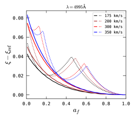
Figure 9: Effects of asymmetric Ly$\alpha$ profiles (Eq. 62) on the required flux rescaling of the selection function for searches with a symmetric 1D Gaussian profile. We plot the difference $\xi-\xi_{\mathrm{ref}}$ as a function of the asymmetry parameter $a_{\mathrm{f}}$ (Eq. 64). The solid lines are the evaluations of the relevant expressions on a grid that is 10-fold sampled with respect to the spectral sampling of MUSE, whereas the dotted lines show the results if the LSF convolved line profile (Eq. 67) is resampled to the MUSE grid (see text for details). The different colours correspond to different intrinsic effective line widths (Eq. 65), with their $v_{\mathrm{FWHM}}$ provided in the legend.

3.3.4 Synthesis for population studies

Above considerations provide us with $C_{\widetilde{S}}(\lambda)$, i.e. the $C$-factor for calculating the selection function (Eq. 32) or the 50% completeness limit (Eq. 33) for a non-template matching source $\widetilde{\bm{S}}$ described by Eq. (38). We recall that $C_{\widetilde{S}}(\lambda)$ can be expressed by a rescaling of $C$-factor (Eq. 44) of the idealised selection function ($C_{\mathcal{I}}(\lambda)$; Sect. 3.1) with the rescaling factor $\xi(\lambda)$ according to Eq. (42). We remark, that the numerical evaluation of the relevant expressions is nearly instant, even when considering the required sub-sampling and re-binning schemes that are needed for dealing with Sérsic type profiles. For the calculation of a realistic selection function for a population of sources it appears thus feasible to consider large ensembles of source templates $\widetilde{S}_{i}$ from some population and then to calculate $C_{\widetilde{S}_{i}}$ for each of those sources. Then, Eq. (32) needs to be evaluated for each $C_{\widetilde{S}_{i}}$ to obtain $f_{C_{\widetilde{S}_{i}}}$, and the final selection function is then given by $f=\sum_{i}w_{i}f_{C_{\widetilde{S}_{i}}}$, where the weights ($\sum_{i}w_{i}\equiv 1$) have to be chosen according to the expected occurrence rate of $\widetilde{S}_{i}$ within the population. Alternatively, the source parameters or profiles are directly drawn from the underlying population, and in this case $f=N^{-1}\sum_{i}f_{C_{\widetilde{S}_{i}}}$, where $N$ is the number of draws. The resulting selection function then provides a robust estimate of the realistic selection function for the catalogue entries of such a population in a IFS data cuboid.

4 Summary and Concluding Remarks

This article presented a discrete matched filtering approach in three dimensions that correctly accounts for rapidly varying variances along one dimension while in the two other dimensions the variances are fixed. The motivation for this approach is the search for faint astronomical emission line signals in wide field integral field spectroscopic datasets. An implementation of the method is provided in an updated version in the open source Python software LSDCat that can be obtained from the Astrophysics Source Code Library: https://ascl.net/1612.002. We demonstrated in this article, by making use of the publicly available MUSE-Wide Data Release 1, that the updated algorithm provides indeed better SN for emission line signals in the spectral vicinity of telluric air-glow lines.

As with the original LSDCat, the matched filtering routines are implemented in lsd_cc_spatial.py and lsd_cc_spectral.py. For lsd_cc_spatial.py, which computes the inner sum of Eq. (27), only a flux data cuboid and the template parameters (A) are needed as input. The outer sum of Eq. (27) is implemented in lsd_cc_spectral.py, and here the resulting temporary cuboid from the inner sum and the effective variance spectrum are required as an input. If desired, the user can still use the classic algorithm (Eq. 19) in order to reproduce results obtained with the original implementation of LSDCat.

We discussed a useful property of the emission line search with a matched-filter, namely that in such a search the selection function is deterministic for a given variance spectrum provided that the noise is behaving according to the expectations. Under this provision the selection function can be expressed by a simple analytic formula (Eq. 32), with a factor of proportionality, $C(\lambda)$, that only depends on the congruence between assumed source profile and actual source profiles. We provide an expression for $C(\lambda)$ for the idealised case where template and source match exactly (Eq. 37).

We also presented ideas regarding how the deterministic selection function for the idealised case can be used to obtain realistic selection functions for line source profiles that are not fully congruent with the template. In particular, we provided a formula that allows to calculate the effect on the factor $C(\lambda)$ for source profiles that differ from the template profiles (Eq. 49). We then analysed three example situations of spatial profile mismatches. We put the idea forward that this method can be extended to obtain realistic selection functions for catalogue entries of a population of emission line sources, where the spatial and spectral properties have been understood in a statistical sense.

Using an algorithm with a deterministic selection function removes the need for computationally cumbersome source insertion and recovery experiments. Moreover, such an algorithm may also be used to efficiently design IFS survey observations. State-of-the art telescope facilities require a reliable estimate of the required exposure time already at the application stage. To this aim interactive exposure time calculators are provided. The calculations of those tools use a model of the detectors and the atmosphere to provide a reliable estimate of the background noise. Such estimates of the background noise could then be used with the here presented approach to predict, e.g., catalogue incidences of particular emission line galaxies given their line luminosity function.

Here we verified the analytic selection function with $C(\lambda)$ for the idealised case against a source insertion experiment. This experiment was carried out in the data cuboid from the deepest MUSE survey ever obtained, the $t_{\mathrm{exp}}=141$ h MUSE eXtreme Deep Field. In this dataset the analytic expression for an idealised selection function, where the sources match the template exactly, shows excellent congruence with a selection function derived from a source insertion and recovery experiment. We remark that the MXDF dataset is somewhat special in the sense that the observing strategy was chosen to homogenise the background noise and to remove any potential residual systematics. Nevertheless, the assumption of spatially invariant noise is also met to a sufficient degree in shallower MUSE data, and it was shown for the standard dithering strategy of the deep MUSE observations of the MUSE Hubble Deep Field South survey (Bacon . 2015) that the noise scales only with some moderate deviation from the expected $1/\sqrt{N_{\mathrm{exp}}}$ behaviour. Nevertheless, a full verification of the here presented approach with shallower data cuboids is desirable in the future.

The assumption of spatially invariant noise will not be met at positions where bright source introduce shot-noise themselves. Even if their flux could be subtracted perfectly, e.g., with the methods presented by Kamann . (2013) for stars and Schmidt . (2019) for galaxies, the spaxels covered by those sources will violate the assumption of a background limited search. Therefore the SN values computed with the methods presented here will be biased low. For population studies, that rely on accurate selection functions it is therefore necessary to identify such regions and to exclude them from the analysis. In MUSE data cuboids this can be achieved, e.g., by visual inspection of the variance cube. However, most of the regions on the sky were searches for faint emission line galaxies are performed, are typically chosen such that the density of bright foreground sources is low.

Some important aspects of the line source detection problem in integral field spectroscopic data were not discussed here. We mention those briefly below.

First, we did not make direct statements regarding the reliability (sometimes also dubbed purity) on the samples from our catalogue. The reliability $R$ is defined as the complement of the false detection probability $p_{\mathrm{F}}$: $R=1-p_{\mathrm{F}}$ (e.g. Hong . 2014). As noted in Sect. 2.1, the standard conversion between $p_{\mathrm{F}}$ and detection threshold is formally not correct. A series of articles addressed this issue in 2D (Vio  Andreani 2016; Vio . 2017; 2019). While the details are mathematically involved, the upshot is that the detection threshold has to be chosen more conservatively than what the standard expectation based on a Gaussian distribution would provide. An often used empirical approach to quantify the reliability is to use negated datasets, which works well under the assumption of the noise being symmetric (see also Serra . 2012).

Second, the construction of the selection function is based on the ground truth for $F_{\mathrm{line}}$, which however is unknown for observed sources, where we measure $F_{\mathrm{line}}^{\mathrm{obs}}\pm\Delta F_{\mathrm{line}}^{\mathrm{obs}}$ to characterise the distribution of possible line fluxes. This needs to be taken into account, when we use the selection function for modelling purposes, and the well known Eddington-Malmquist bias in luminosity function determinations results from this effect (e.g., Chapter 5.5 in Ivezić . 2014). One way to avoid such biases are additional cuts of the sample by only using sources where the errors on the flux measurements do not correspond to significant changes in the selection function, i.e., where $f_{C}(F_{\mathrm{line}}^{\mathrm{obs}}\pm\Delta F_{\mathrm{line}}^{\mathrm{obs}},\lambda)\simeq f_{C}(F_{\mathrm{line}}^{\mathrm{obs}},\lambda)$. However, this may drastically reduce the sample, and an alternative is to account for the measurement errors in the modelling process (Rix . 2021).

Last, a current bottleneck in the construction of line emitter catalogues based on wide-field IFS data is the manual classification step. Related to this are spurious line signals due to imperfect continuum subtraction of sources with significant continuum emission. These residuals also have to be weeded out manually from catalogues. We advocate future research on those latter issues by investigating machine learning techniques for classification and better continuum subtraction methods that do not leave strong residuals (see Kamann . 2013; Schmidt . 2019).

While matched filtering is a useful method to uncover the faintest emission line galaxies in wide-field IFS datasets, ultimately it is only the first step in the detection and analysis chain, and subsequent steps are required before astrophysical facts can be inferred from the data. Arguably, however, a good understanding of this first step in the chain is required for successful statistical analyses of IFS survey data.

Appendix A Description of the templates used in LSDCat

For completeness and in order to contextualise the template parameters introduced in Sect. 3 we provide here a short description of the 3D template S used in LSDCat. A more comprehensive description is provided in HW17.

LSDCat templates are optimised for spatially unresolved sources in ground based observations. The spatial profile of such an emission line source can either be approximated by a circular symmetric Gaussian,

$$S_{x,y}(\lambda)=\frac{1}{2\pi\sigma_{\mathrm{G}}^{2}(\lambda)}\exp\left(-\frac{x^{2}+y^{2}}{2\sigma_{\mathrm{G}}^{2}(\lambda)}\right)\;\text{,}$$ (69)

with the dispersion $\sigma_{\mathrm{G}}$, or by a Moffat (1969) profile,

$$S_{x,y}(\lambda)=\frac{\beta-1}{\pi r_{\mathrm{d}}^{2}(\lambda)}\left[1+\frac{x^{2}+y^{2}}{r_{\mathrm{d}}^{2}(\lambda)}\right]^{-\beta}\;\text{,}$$ (70)

with the width parameter $r_{\mathrm{d}}$ and the kurtosis parameter $\beta$. We remark that equation (70) in the limit $\beta\rightarrow\infty$ is identical to Eq. (69) (Trujillo . 20012).

The dependence on wavelength $\lambda$ of $\sigma_{\mathrm{G}}$ in Eq. (69) or $r_{\mathrm{d}}$ in Eq. (70) is required, since the spatial resolution of ground based observations is wavelength dependent (see, e.g., Hickson 2014). Here this wavelength dependence of the point-spread function is empirically modelled by a polynomial,

$$\mathrm{FWHM}(\lambda)[\text{${}^{\prime\prime}$}]=\sum_{i=0}^{N_{p}}p_{i}(\lambda-\lambda_{0})^{i}\;\text{,}$$ (71)

and already a quadratic polynomial ($N_{p}=2$) provides quite an accurate description over the optical wavelength range. The relation between the full width at half maximum (FWHM in Eq. 71) and $\sigma_{\mathrm{G}}$ in Eq. (69) is $\sigma_{\mathrm{G}}=\mathrm{FWHM}/(2\,\sqrt{2\ln 2})$, whereas for the width parameter $r_{d}$ in Eq. (70) we have $r_{\mathrm{d}}=\mathrm{FWHM}/\left(2\,\sqrt{2^{1/\beta}-1}\right)$. Several empirical ways to determine optimal values for the $p_{i}$ in Eq. (71) have been developed for MUSE observations (see, e.g., Herenz . 2017; Bacon . 2017; Urrutia . 2019). Moreover, for MUSE observations with laser-assisted ground layer adaptive optics the wavelength dependence of the Moffat function can be modelled from data provided by the adaptive optics telemetry system (Oberti . 2018) with the muse-psfr software (Fusco . 2020).

We point out that the here adopted convention for the polynomial description of the $\lambda$-dependence Eq. (71) differs from the convention in the MUSE Python data analysis framework and in muse-psfr. The recipe for conversion is provided in B. Lastly, we note that the parameter $\beta$ in Eq. (70) is usually not strongly dependent on wavelength, but in LSDCat also a polynomial analogous to Eq. (71) can be used to enforce a wavelength dependence on $\beta$ if desired.

The spectral profile is modelled as a simple 1D Gaussian

$$S_{z}=\frac{1}{\sqrt{2\pi}\sigma_{z}}\exp\left(-\frac{z^{2}}{2\sigma_{z}^{2}}\right)\;\text{,}$$ (72)

whose width $\sigma_{v}$ (in km s^-1)is fixed in velocity space. For the linear sampled wavelength grid,

$$\lambda=z\cdot\Delta\lambda+\lambda_{z=0}\;\text{,}$$ (73)

thus

$$\sigma_{z}=\frac{\sigma_{v}}{c}\left(\frac{\lambda_{z=0}}{\Delta\lambda}+z\right)\;\text{.}$$ (74)

Here $\lambda_{z=0}$ denotes the wavelength at the first spectral bin ($z=0$) and $\Delta\lambda$ denotes the wavelength increment per spectral bin ($\Delta\lambda=1.25$Å is the default spectral increment for MUSE).

Appendix B Conversion of polynomial coefficients used in MPDAF and muse-psfr for use in LSDCat

The MUSE Python analysis framework (MPDAF; Bacon . 2016; Piqueras . 2017) and muse-psfr (Fusco . 2020) can model the wavelength dependence of the width parameter of the Moffat function (Eq. 70). However, the empirical polynomial model adopted by those tools is written as

$$q(\lambda)=\sum_{i=0}^{N_{p}}b_{i}\left(\frac{\lambda-\lambda_{1}}{\lambda_{2}-\lambda_{1}}-\frac{1}{2}\right)\;\text{,}$$ (75)

whereas in LSDCat we adopt

$$p(\lambda)=\sum_{i=0}^{N_{p}}a_{i}(\lambda-\lambda_{0})^{i}$$ (76)

(cf. Eq. 71). Clearly, Eq. (76) provides a more intuitive description of the wavelength dependence, since $a_{0}$ refers to the parameter under consideration (FWHM or $\beta$) at $\lambda_{0}$ (in Å). On the other hand, Eq. (75) appears numerically more accurate since $q$ evaluates on the interval $[-1,1]$ where the density of digitally stored floating point numbers is highest. However, this extra level of numerical accuracy appears not to provide practical benefits, at least for the use in LSDCat. Using the Heaviside step function,

$$\Theta(k)=\begin{cases}1&(k\leq 0)\\ 0&(k>0)\end{cases}\;\text{,}$$ (77)

we can achieve the conversion of the $b_{i}$ in Eq. (75) to the $a_{i}$ in Eq. (76) via

$$a_{i}=\sum_{j=0}^{N_{p}}c_{j}\,\binom{j}{i}\,\lambda_{0}^{i-j}\,\Theta(j-i)$$ (78)

with

$$c_{i}=\sum_{j=0}^{N_{p}}b_{j}\,\binom{j}{i}\alpha^{i}\beta^{i-j}\,\Theta(j-i)\;\text{,}$$ (79)

where $\alpha$ and $\beta$ in Eq. (79) are shorthands for

$$\alpha=\frac{1}{\lambda_{2}-\lambda_{1}}\quad\text{and}\quad\beta=-\left(\frac{\lambda_{1}}{\lambda_{2}-\lambda_{1}}+\frac{1}{2}\right)\,\text{.}$$ (80)

Appendix C Template parameters used in the numerical examples

Table 1:   Parameters describing the 3D Gaussian template used in for the LAE search MXDF (see A for the parameterisation). For the spatial domain the FWHM-$\lambda$ dependence is given as polynomaial coefficients of Eq. (71) with $\lambda_{0}=7050$Å.

spatial domain
$p_{i}$	FWHM [′′Å-i]
$p_{1}$	1.0042
$p_{2}$	$-3.322\times 10^{-5}$
spectral domain
$v_{\mathrm{FWHM}}$	250 km s-1

Table 2:  Polynomial coefficients in Eq. (76) for $\lambda_{0}=7000$ Å that describe the wavelength dependence of a Moffat point-spread function model in the MXDF (Bacon . 2022) according to muse-psfr (Fusco . 2020).

$p_{i}$	FWHM [′′Å-i]	$\beta$
$p_{0}$	0.49	1.96
$p_{1}$	$-5.69\times 10^{-5}$	$-1.02\times 10^{-4}$
$p_{2}$	$\phantom{-}1.14\times 10^{-9}$	$\phantom{-}6.52\times 10^{-10}$
$p_{3}$	$\phantom{-}1.06\times 10^{-12}$	$\phantom{-}5.43\times 10^{-12}$
$p_{4}$	$-8.86\times 10^{-17}$	$-1.54\times 10^{-15}$
$p_{5}$	$\phantom{-}2.91\times 10^{-19}$	$-3.75\times 10^{-19}$

For reference we list in Table 1 and Table 2 the template parameters that have been used for the calculations in Sect. 3. The templates and their parameterisations are listed in A.

Table 1 lists the parameters of the 3D Gaussian template that have been used for a search of Ly$\alpha$ emitting galaxies (Herenz et al., in prep.) in the recently released data cuboid of the MXDF (Bacon et al. 2022). These parameters were chosen to maximise the SN of known Ly$\alpha$ emitters from the previous MUSE Ultra Deep Field survey (Inami . 2017) where the footprint of the MXDF is located. As detection threshold we used $SN_{\mathrm{thresh}}=6.41$. This template was used in the example of Sect. 3.2, where we compute the idealised selection function at $\lambda>8500$ Å with Eq. (32) and $C_{\mathcal{I}}(\lambda)$ from Eq. (37) and where we contrasted the analytical calculation to a source insertion and recovery experiment.

Table 2 lists the polynomial coefficients that describe the wavelength dependence of the Moffat muse-psfr (Fusco . 2020) point spread function model in the MXDF according to Eq. (76) with $\lambda_{0}=7000$ Å. The muse-psfr tool uses data that was recorded by the adaptive optics telemetry system (Oberti . 2018) during the observations. The polynomial coefficients are given in the header of the FITS file of the MXDF datacube, but for the expression in Eq. (75). We here use the formalism provided in B to convert them into the more natural form of Eq. (76).

Author Biography

Edmund Christian Herenz is interested in extragalactic astrophysics and cosmology. He obtained his PhD in 2016 from the University Potsdam for his thesis “Detecting and understanding extragalactic Lyman $\alpha$ emission using 3D spectroscopy” that was supervised by Lutz Wisotzki and Martin Roth at the Leibniz-Institute for Astrophysics Potsdam (AIP). Afterwards he did a Post-Doc with Matthew Hayes at Stockholm University. He was then awarded with a Fellowship from the European Southern Observatory where he supported operations of HAWK-I and MUSE at UT4 “Yepun”. He currently spends the 4th year of ESO Chile fellowship as a visiting researcher at the Leiden Observatory (Leiden University) in the Netherlands.

References

- Allington-Smith (\APACyear2006) \APACinsertmetastarAllington-Smith2006{APACrefauthors}Allington-Smith, J. \APACrefYearMonthDay2006\APACmonth06, \APACjournalVolNumPagesNew A Rev.50244-251. {APACrefDOI} 10.1016/j.newar.2006.02.024 \PrintBackRefs\CurrentBib
- Astropy Collaboration \BOthers. (\APACyear2022) \APACinsertmetastarAstropyCollaboration2022{APACrefauthors}Astropy Collaboration, Price-Whelan, A\BPBIM., Lim, P\BPBIL. et al. \APACrefYearMonthDay2022\APACmonth08, \APACjournalVolNumPagesApJ9352167. {APACrefDOI} 10.3847/1538-4357/ac7c74 \PrintBackRefs\CurrentBib
- Bacon \BOthers. (\APACyear2002) \APACinsertmetastarBacon2002{APACrefauthors}Bacon, R., Adam, G., Cabrit, S. et al. \APACrefYearMonthDay2002\APACmonth01, \BBOQ\APACrefatitleA Mega Integral Field Spectrograph for the VLT A Mega Integral Field Spectrograph for the VLT.\BBCQ \BIn J. Bergeron \BBA G. Monnet (\BEDS), \APACrefbtitleScientific Drivers for ESO Future VLT/VLTI Instrumentation Scientific Drivers for ESO Future VLT/VLTI Instrumentation \BPG 108. {APACrefDOI} 10.1007/10857019_17 \PrintBackRefs\CurrentBib
- Bacon \BOthers. (\APACyear2022) \APACinsertmetastarBacon2022{APACrefauthors}Bacon, R., Brinchmann, J., Conseil, S. et al. \APACrefYearMonthDay2022\APACmonth11, \APACjournalVolNumPagesarXiv e-printsarXiv:2211.08493. \PrintBackRefs\CurrentBib
- Bacon \BOthers. (\APACyear2015) \APACinsertmetastarBacon2015{APACrefauthors}Bacon, R., Brinchmann, J., Richard, J. et al. \APACrefYearMonthDay2015\APACmonth03, \APACjournalVolNumPagesA&A575A75. {APACrefDOI} 10.1051/0004-6361/201425419 \PrintBackRefs\CurrentBib
- Bacon \BOthers. (\APACyear2017) \APACinsertmetastarBacon2017{APACrefauthors}Bacon, R., Conseil, S., Mary, D. et al. \APACrefYearMonthDay2017\APACmonth11, \APACjournalVolNumPagesA&A608A1. {APACrefDOI} 10.1051/0004-6361/201730833 \PrintBackRefs\CurrentBib
- Bacon \BOthers. (\APACyear2021) \APACinsertmetastarBacon2021{APACrefauthors}Bacon, R., Mary, D., Garel, T. et al. \APACrefYearMonthDay2021\APACmonth03, \APACjournalVolNumPagesA&A647A107. {APACrefDOI} 10.1051/0004-6361/202039887 \PrintBackRefs\CurrentBib
- Bacon \BBA Monnet (\APACyear2017) \APACinsertmetastarBacon2017a{APACrefauthors}Bacon, R.\BCBT \BBA Monnet, G\BPBIJ. \APACrefYear2017, \APACrefbtitleOptical 3D-Spectroscopy for Astronomy Optical 3D-Spectroscopy for Astronomy. \APACaddressPublisherWiley-VCH Verlag GmbH & Co. KGaA. {APACrefDOI} 10.1002/9783527674824 \PrintBackRefs\CurrentBib
- Bacon \BOthers. (\APACyear2016) \APACinsertmetastarBacon2016{APACrefauthors}Bacon, R., Piqueras, L., Conseil, S., Richard, J.\BCBL \BBA Shepherd, M. \APACrefYearMonthDay2016\APACmonth11, \APACrefbtitleMPDAF: MUSE Python Data Analysis Framework. MPDAF: MUSE Python Data Analysis Framework., \APAChowpublishedAstrophysics Source Code Library. \PrintBackRefs\CurrentBib
- Bacon \BOthers. (\APACyear2014) \APACinsertmetastarBacon2014{APACrefauthors}Bacon, R., Vernet, J., Borisiva, E. et al. \APACrefYearMonthDay2014\APACmonth09, \APACjournalVolNumPagesThe Messenger15713-16. \PrintBackRefs\CurrentBib
- Blanc \BOthers. (\APACyear2011) \APACinsertmetastarBlanc2011{APACrefauthors}Blanc, G\BPBIA., Adams, J\BPBIJ., Gebhardt, K. et al. \APACrefYearMonthDay2011\APACmonth07, \APACjournalVolNumPagesApJ73631. {APACrefDOI} 10.1088/0004-637X/736/1/31 \PrintBackRefs\CurrentBib
- Bourguignon \BOthers. (\APACyear2012) \APACinsertmetastarBourguignon2012{APACrefauthors}Bourguignon, S., Mary, D.\BCBL \BBA Slezak, É. \APACrefYearMonthDay2012\APACmonth01, \APACjournalVolNumPagesStatistical Methodology91-232–43. {APACrefURL} https://doi.org/10.1016/j.stamet.2011.04.010 {APACrefDOI} 10.1016/j.stamet.2011.04.010 \PrintBackRefs\CurrentBib
- Caditz (\APACyear2016) \APACinsertmetastarCaditz2016{APACrefauthors}Caditz, D\BPBIM. \APACrefYearMonthDay2016\APACmonth11, \APACjournalVolNumPagesApJ83150. {APACrefDOI} 10.3847/0004-637X/831/1/50 \PrintBackRefs\CurrentBib
- Childs \BBA Stanway (\APACyear2018) \APACinsertmetastarChilds2018{APACrefauthors}Childs, H\BPBIJ\BPBIT.\BCBT \BBA Stanway, E\BPBIR. \APACrefYearMonthDay2018\APACmonth10, \APACjournalVolNumPagesMNRAS4801938-1949. {APACrefDOI} 10.1093/mnras/sty1974 \PrintBackRefs\CurrentBib
- Das (\APACyear1991) \APACinsertmetastarDas1991{APACrefauthors}Das, P\BPBIK. \APACrefYear1991, \APACrefbtitleOptical Signal Processing Optical Signal Processing. \APACaddressPublisherSpringer Science + Business Media. {APACrefURL} http://dx.doi.org/10.1007/978-3-642-74962-9 {APACrefDOI} 10.1007/978-3-642-74962-9 \PrintBackRefs\CurrentBib
- Dijkstra (\APACyear2019) \APACinsertmetastarDijkstra2017{APACrefauthors}Dijkstra, M. \APACrefYearMonthDay2019Jan, \APACjournalVolNumPagesSaas-Fee Advanced Course461. {APACrefDOI} 10.1007/978-3-662-59623-4_1 \PrintBackRefs\CurrentBib
- Ferruit (\APACyear2010) \APACinsertmetastarFerruit2010{APACrefauthors}Ferruit, P. \APACrefYearMonthDay2010\APACmonth01, \BBOQ\APACrefatitleAnalysis of 3D data Analysis of 3D data.\BBCQ \BIn E. Mediavilla, S. Arribas, M. Roth\BCBL \BOthers. (\BEDS), \APACrefbtitle3D Spectroscopy in Astronomy 3D Spectroscopy in Astronomy \BPGS 126–157. \APACaddressPublisherCambridgeCambridge University Press. \PrintBackRefs\CurrentBib
- Fusco \BOthers. (\APACyear2020) \APACinsertmetastarFusco2020{APACrefauthors}Fusco, T., Bacon, R., Kamann, S. et al. \APACrefYearMonthDay2020\APACmonth03, \APACjournalVolNumPagesA&A635A208. {APACrefDOI} 10.1051/0004-6361/202037595 \PrintBackRefs\CurrentBib
- Gebhardt \BOthers. (\APACyear2021) \APACinsertmetastarGebhardt2021{APACrefauthors}Gebhardt, K., Mentuch Cooper, E., Ciardullo, R. et al. \APACrefYearMonthDay2021\APACmonth12, \APACjournalVolNumPagesApJ9232217. {APACrefDOI} 10.3847/1538-4357/ac2e03 \PrintBackRefs\CurrentBib
- Ginolfi \BOthers. (\APACyear2022) \APACinsertmetastarGinolfi2022{APACrefauthors}Ginolfi, M., Piconcelli, E., Zappacosta, L. et al. \APACrefYearMonthDay2022\APACmonth08, \APACjournalVolNumPagesNature Communications134574. {APACrefDOI} 10.1038/s41467-022-32297-x \PrintBackRefs\CurrentBib
- Graham \BBA Driver (\APACyear2005) \APACinsertmetastarGraham2005{APACrefauthors}Graham, A\BPBIW.\BCBT \BBA Driver, S\BPBIP. \APACrefYearMonthDay2005, \APACjournalVolNumPagesPASA22118-127. {APACrefDOI} 10.1071/AS05001 \PrintBackRefs\CurrentBib
- Green \BOthers. (\APACyear2022) \APACinsertmetastarGreen2022{APACrefauthors}Green, R\BPBIF., Luginbuhl, C\BPBIB., Wainscoat, R\BPBIJ.\BCBL \BBA Duriscoe, D. \APACrefYearMonthDay2022\APACmonth12, \APACjournalVolNumPagesA&A Rev.3011. {APACrefDOI} 10.1007/s00159-021-00138-3 \PrintBackRefs\CurrentBib
- Hanuschik (\APACyear2003) \APACinsertmetastarHanuschik2003{APACrefauthors}Hanuschik, R\BPBIW. \APACrefYearMonthDay2003\APACmonth09, \APACjournalVolNumPagesA&A4071157-1164. {APACrefDOI} 10.1051/0004-6361:20030885 \PrintBackRefs\CurrentBib
- Hayes \BOthers. (\APACyear2013) \APACinsertmetastarHayes2013{APACrefauthors}Hayes, M., Östlin, G., Schaerer, D. et al. \APACrefYearMonthDay2013\APACmonth03, \APACjournalVolNumPagesApJ765L27. {APACrefDOI} 10.1088/2041-8205/765/2/L27 \PrintBackRefs\CurrentBib
- Herenz (\APACyear2022) \APACinsertmetastar2022joks.confE..12H{APACrefauthors}Herenz, E\BPBIC. \APACrefYearMonthDay2022\APACmonth04, \BBOQ\APACrefatitleTowards LSDCat2.0: An improved algorithm for detecting emission line sources in integral-field spectroscopic datasets Towards LSDCat2.0: An improved algorithm for detecting emission line sources in integral-field spectroscopic datasets.\BBCQ \BIn \APACrefbtitleJoint Observatories Kavli Science Forum in Chile (joksfic2022). Proceedings of the conference held 25-29 April Joint Observatories Kavli Science Forum in Chile (joksfic2022). Proceedings of the conference held 25-29 April \BPG 12. {APACrefDOI} 10.5281/zenodo.6547643 \PrintBackRefs\CurrentBib
- Herenz \BOthers. (\APACyear2017) \APACinsertmetastarHerenz2017a{APACrefauthors}Herenz, E\BPBIC., Urrutia, T., Wisotzki, L. et al. \APACrefYearMonthDay2017\APACmonth09, \APACjournalVolNumPagesA&A606A12. {APACrefDOI} 10.1051/0004-6361/201731055 \PrintBackRefs\CurrentBib
- Herenz \BBA Wisotzki (\APACyear2017) \APACinsertmetastarHerenz2017{APACrefauthors}Herenz, E\BPBIC.\BCBT \BBA Wisotzki, L. \APACrefYearMonthDay2017\APACmonth06, \APACjournalVolNumPagesA&A602A111. {APACrefDOI} 10.1051/0004-6361/201629507 \PrintBackRefs\CurrentBib
- Herenz \BOthers. (\APACyear2019) \APACinsertmetastarHerenz2019{APACrefauthors}Herenz, E\BPBIC., Wisotzki, L., Saust, R. et al. \APACrefYearMonthDay2019\APACmonth01, \APACjournalVolNumPagesA&A621A107. {APACrefDOI} 10.1051/0004-6361/201834164 \PrintBackRefs\CurrentBib
- Herrero Alonso \BOthers. (\APACyear2021) \APACinsertmetastarHerreroAlonso2021{APACrefauthors}Herrero Alonso, Y., Krumpe, M., Wisotzki, L. et al. \APACrefYearMonthDay2021\APACmonth09, \APACjournalVolNumPagesA&A653A136. {APACrefDOI} 10.1051/0004-6361/202141226 \PrintBackRefs\CurrentBib
- Hickson (\APACyear2014) \APACinsertmetastarHickson2014{APACrefauthors}Hickson, P. \APACrefYearMonthDay2014\APACmonth11, \APACjournalVolNumPagesA&A Rev.2276. {APACrefDOI} 10.1007/s00159-014-0076-9 \PrintBackRefs\CurrentBib
- Hill \BOthers. (\APACyear2021) \APACinsertmetastarHill2021{APACrefauthors}Hill, G\BPBIJ., Lee, H., MacQueen, P\BPBIJ. et al. \APACrefYearMonthDay2021\APACmonth12, \APACjournalVolNumPagesAJ1626298. {APACrefDOI} 10.3847/1538-3881/ac2c02 \PrintBackRefs\CurrentBib
- Hong \BOthers. (\APACyear2014) \APACinsertmetastarHong2014{APACrefauthors}Hong, S., Dey, A.\BCBL \BBA Prescott, M\BPBIK\BPBIM. \APACrefYearMonthDay2014\APACmonth11, \APACjournalVolNumPagesPASP1261048-1067. {APACrefDOI} 10.1086/679285 \PrintBackRefs\CurrentBib
- Inami \BOthers. (\APACyear2017) \APACinsertmetastarInami2017{APACrefauthors}Inami, H., Bacon, R., Brinchmann, J. et al. \APACrefYearMonthDay2017\APACmonth11, \APACjournalVolNumPagesA&A608A2. {APACrefDOI} 10.1051/0004-6361/201731195 \PrintBackRefs\CurrentBib
- Ivezić \BOthers. (\APACyear2014) \APACinsertmetastarIvezic2014{APACrefauthors}Ivezić, Ž., Connelly, A\BPBIJ., VanderPlas, J\BPBIT.\BCBL \BBA Gray, A. \APACrefYear2014, \APACrefbtitleStatistics, Data Mining, and Machine Learningin Astronomy Statistics, Data Mining, and Machine Learningin Astronomy. \PrintBackRefs\CurrentBib
- Jaranowski \BBA Królak (\APACyear2012) \APACinsertmetastarJaranowski2012{APACrefauthors}Jaranowski, P.\BCBT \BBA Królak, A. \APACrefYearMonthDay2012\APACmonth03, \APACjournalVolNumPagesLiving Reviews in Relativity1514. {APACrefDOI} 10.12942/lrr-2012-4 \PrintBackRefs\CurrentBib
- Kamann \BOthers. (\APACyear2013) \APACinsertmetastarKamann2013{APACrefauthors}Kamann, S., Wisotzki, L.\BCBL \BBA Roth, M\BPBIM. \APACrefYearMonthDay2013\APACmonth01, \APACjournalVolNumPagesA&A549A71. {APACrefDOI} 10.1051/0004-6361/201220476 \PrintBackRefs\CurrentBib
- Laursen \BOthers. (\APACyear2011) \APACinsertmetastarLaursen2011{APACrefauthors}Laursen, P., Sommer-Larsen, J.\BCBL \BBA Razoumov, A\BPBIO. \APACrefYearMonthDay2011\APACmonth02, \APACjournalVolNumPagesApJ72852. {APACrefDOI} 10.1088/0004-637X/728/1/52 \PrintBackRefs\CurrentBib
- Leclercq \BOthers. (\APACyear2017) \APACinsertmetastarLeclercq2017{APACrefauthors}Leclercq, F., Bacon, R., Wisotzki, L. et al. \APACrefYearMonthDay2017\APACmonth11, \APACjournalVolNumPagesA&A608A8. {APACrefDOI} 10.1051/0004-6361/201731480 \PrintBackRefs\CurrentBib
- Loomis \BOthers. (\APACyear2018) \APACinsertmetastarLoomis2018{APACrefauthors}Loomis, R\BPBIA., Öberg, K\BPBII., Andrews, S\BPBIM., Walsh, C., Czekala, I., Huang, J.\BCBL \BBA Rosenfeld, K\BPBIA. \APACrefYearMonthDay2018\APACmonth04, \APACjournalVolNumPagesAJ155182. {APACrefDOI} 10.3847/1538-3881/aab604 \PrintBackRefs\CurrentBib
- Lujan Niemeyer \BOthers. (\APACyear2022) \APACinsertmetastarLujanNiemeyer2022{APACrefauthors}Lujan Niemeyer, M., Komatsu, E., Byrohl, C. et al. \APACrefYearMonthDay2022\APACmonth04, \APACjournalVolNumPagesApJ929190. {APACrefDOI} 10.3847/1538-4357/ac5cb8 \PrintBackRefs\CurrentBib
- Mallery \BOthers. (\APACyear2012) \APACinsertmetastarMallery2012{APACrefauthors}Mallery, R\BPBIP., Mobasher, B., Capak, P. et al. \APACrefYearMonthDay2012\APACmonth12, \APACjournalVolNumPagesApJ760128. {APACrefDOI} 10.1088/0004-637X/760/2/128 \PrintBackRefs\CurrentBib
- Mary \BOthers. (\APACyear2020) \APACinsertmetastarMary2020{APACrefauthors}Mary, D., Bacon, R., Conseil, S., Piqueras, L.\BCBL \BBA Schutz, A. \APACrefYearMonthDay2020\APACmonth03, \APACjournalVolNumPagesA&A635A194. {APACrefDOI} 10.1051/0004-6361/201937001 \PrintBackRefs\CurrentBib
- Mas-Ribas \BBA Dijkstra (\APACyear2016) \APACinsertmetastarMas-Ribas2016{APACrefauthors}Mas-Ribas, L.\BCBT \BBA Dijkstra, M. \APACrefYearMonthDay2016\APACmonth05, \APACjournalVolNumPagesApJ82284. {APACrefDOI} 10.3847/0004-637X/822/2/84 \PrintBackRefs\CurrentBib
- Maseda \BOthers. (\APACyear2018) \APACinsertmetastarMaseda2018{APACrefauthors}Maseda, M\BPBIV., Bacon, R., Franx, M. et al. \APACrefYearMonthDay2018\APACmonth09, \APACjournalVolNumPagesApJ865L1. {APACrefDOI} 10.3847/2041-8213/aade4b \PrintBackRefs\CurrentBib
- Meillier \BOthers. (\APACyear2016) \APACinsertmetastarMeillier2016{APACrefauthors}Meillier, C., Chatelain, F., Michel, O., Bacon, R., Piqueras, L., Bacher, R.\BCBL \BBA Ayasso, H. \APACrefYearMonthDay2016\APACmonth04, \APACjournalVolNumPagesA&A588A140. {APACrefDOI} 10.1051/0004-6361/201527724 \PrintBackRefs\CurrentBib
- Moffat (\APACyear1969) \APACinsertmetastarMoffat1969{APACrefauthors}Moffat, A\BPBIF\BPBIJ. \APACrefYearMonthDay1969\APACmonth12, \APACjournalVolNumPagesA&A3455. \PrintBackRefs\CurrentBib
- Morrissey \BOthers. (\APACyear2018) \APACinsertmetastarMorrissey2018{APACrefauthors}Morrissey, P., Matuszewski, M., Martin, D\BPBIC. et al. \APACrefYearMonthDay2018\APACmonth09, \APACjournalVolNumPagesApJ86493. {APACrefDOI} 10.3847/1538-4357/aad597 \PrintBackRefs\CurrentBib
- Noll \BOthers. (\APACyear2012) \APACinsertmetastarNoll2012{APACrefauthors}Noll, S., Kausch, W., Barden, M., Jones, A\BPBIM., Szyszka, C., Kimeswenger, S.\BCBL \BBA Vinther, J. \APACrefYearMonthDay2012\APACmonth07, \APACjournalVolNumPagesA&A543A92. {APACrefDOI} 10.1051/0004-6361/201219040 \PrintBackRefs\CurrentBib
- Oberti \BOthers. (\APACyear2018) \APACinsertmetastarOberti2018{APACrefauthors}Oberti, S., Kolb, J., Madec, P\BHBIY. et al. \APACrefYearMonthDay2018\APACmonth07, \BBOQ\APACrefatitleThe AO in AOF The AO in AOF.\BBCQ \BIn L\BPBIM. Close, L. Schreiber\BCBL \BBA D. Schmidt (\BEDS), \APACrefbtitleAdaptive Optics Systems VI Adaptive Optics Systems VI \BVOL 10703, \BPG 107031G. {APACrefDOI} 10.1117/12.2314055 \PrintBackRefs\CurrentBib
- Ouchi (\APACyear2019) \APACinsertmetastarOuchi2019{APACrefauthors}Ouchi, M. \APACrefYearMonthDay2019\APACmonth01, \APACjournalVolNumPagesSaas-Fee Advanced Course46189. {APACrefDOI} 10.1007/978-3-662-59623-4_3 \PrintBackRefs\CurrentBib
- Pasquini \BOthers. (\APACyear2018) \APACinsertmetastarPasquini2018{APACrefauthors}Pasquini, L., Delabre, B., Ellis, R\BPBIS., Marrero, J., Cavaller, L.\BCBL \BBA de Zeeuw, T. \APACrefYearMonthDay2018\APACmonth08, \BBOQ\APACrefatitleESO Spectroscopic Facility ESO Spectroscopic Facility.\BBCQ \BIn C. Chiappini, I. Minchev, E. Starkenburg\BCBL \BOthers. (\BEDS), \APACrefbtitleRediscovering Our Galaxy Rediscovering Our Galaxy \BVOL 334, \BPG 242-247. {APACrefDOI} 10.1017/S174392131700847X \PrintBackRefs\CurrentBib
- Peng \BOthers. (\APACyear2002) \APACinsertmetastarPeng2002{APACrefauthors}Peng, C\BPBIY., Ho, L\BPBIC., Impey, C\BPBID.\BCBL \BBA Rix, H\BHBIW. \APACrefYearMonthDay2002\APACmonth07, \APACjournalVolNumPagesAJ1241266-293. {APACrefDOI} 10.1086/340952 \PrintBackRefs\CurrentBib
- Piqueras \BOthers. (\APACyear2017) \APACinsertmetastarPiqueras2017{APACrefauthors}Piqueras, L., Conseil, S., Shepherd, M., Bacon, R., Leclercq, F.\BCBL \BBA Richard, J. \APACrefYearMonthDay2017\APACmonth10, \PrintBackRefs\CurrentBib
- Ramos \BOthers. (\APACyear2011) \APACinsertmetastarRamos2011{APACrefauthors}Ramos, E\BPBIP\BPBIR\BPBIG., Vio, R.\BCBL \BBA Andreani, P. \APACrefYearMonthDay2011\APACmonth04, \APACjournalVolNumPagesA&A528A75. {APACrefDOI} 10.1051/0004-6361/201015586 \PrintBackRefs\CurrentBib
- Rhoads \BOthers. (\APACyear2003) \APACinsertmetastarRhoads2003{APACrefauthors}Rhoads, J\BPBIE., Dey, A., Malhotra, S. et al. \APACrefYearMonthDay2003\APACmonth03, \APACjournalVolNumPagesAJ1251006-1013. {APACrefDOI} 10.1086/346272 \PrintBackRefs\CurrentBib
- Richard \BOthers. (\APACyear2019) \APACinsertmetastarRichard2019{APACrefauthors}Richard, J., Bacon, R., Blaizot, J. et al. \APACrefYearMonthDay2019\APACmonth06, \APACjournalVolNumPagesarXiv e-printsarXiv:1906.01657. \PrintBackRefs\CurrentBib
- Rix \BOthers. (\APACyear2021) \APACinsertmetastarRix2021{APACrefauthors}Rix, H\BHBIW., Hogg, D\BPBIW., Boubert, D. et al. \APACrefYearMonthDay2021\APACmonth10, \APACjournalVolNumPagesAJ1624142. {APACrefDOI} 10.3847/1538-3881/ac0c13 \PrintBackRefs\CurrentBib
- Robertson (\APACyear2017) \APACinsertmetastarRobertson2017{APACrefauthors}Robertson, J\BPBIG. \APACrefYearMonthDay2017\APACmonth08, \APACjournalVolNumPagesPASA34e035. {APACrefDOI} 10.1017/pasa.2017.29 \PrintBackRefs\CurrentBib
- Sánchez Almeida \BOthers. (\APACyear2022) \APACinsertmetastarSanchezAlmeida2022{APACrefauthors}Sánchez Almeida, J., Calhau, J., Muñoz-Tuñón, C., González-Morán, A\BPBIL.\BCBL \BBA Rodríguez-Espinosa, J\BPBIM. \APACrefYearMonthDay2022\APACmonth08, \APACjournalVolNumPagesApJ9342100. {APACrefDOI} 10.3847/1538-4357/ac7319 \PrintBackRefs\CurrentBib
- Schmidt \BOthers. (\APACyear2019) \APACinsertmetastarSchmidt2019{APACrefauthors}Schmidt, K\BPBIB., Wisotzki, L., Urrutia, T. et al. \APACrefYearMonthDay2019\APACmonth08, \APACjournalVolNumPagesA&A628A91. {APACrefDOI} 10.1051/0004-6361/201935857 \PrintBackRefs\CurrentBib
- Schwartz \BBA Shaw (\APACyear1975) \APACinsertmetastarSchwartz1975{APACrefauthors}Schwartz, M.\BCBT \BBA Shaw, L. \APACrefYear1975, \APACrefbtitleSignal processing: discrete spectral analysis, detection, and estimation Signal processing: discrete spectral analysis, detection, and estimation. \APACaddressPublisherTokyoMcGraw-Hill Kogakusha, Ltd. \PrintBackRefs\CurrentBib
- Serra \BOthers. (\APACyear2012) \APACinsertmetastarSerra2012{APACrefauthors}Serra, P., Jurek, R.\BCBL \BBA Flöer, L. \APACrefYearMonthDay2012\APACmonth02, \APACjournalVolNumPagesPASA29296-300. {APACrefDOI} 10.1071/AS11065 \PrintBackRefs\CurrentBib
- Sersic (\APACyear1968) \APACinsertmetastarSersic1968{APACrefauthors}Sersic, J\BPBIL. \APACrefYear1968, \APACrefbtitleAtlas de Galaxias Australes Atlas de Galaxias Australes. \PrintBackRefs\CurrentBib
- Shibuya \BOthers. (\APACyear2014) \APACinsertmetastarShibuya2014{APACrefauthors}Shibuya, T., Ouchi, M., Nakajima, K. et al. \APACrefYearMonthDay2014\APACmonth06, \APACjournalVolNumPagesApJ78874. {APACrefDOI} 10.1088/0004-637X/788/1/74 \PrintBackRefs\CurrentBib
- Steidel \BOthers. (\APACyear2011) \APACinsertmetastarSteidel2011{APACrefauthors}Steidel, C\BPBIC., Bogosavljević, M., Shapley, A\BPBIE., Kollmeier, J\BPBIA., Reddy, N\BPBIA., Erb, D\BPBIK.\BCBL \BBA Pettini, M. \APACrefYearMonthDay2011\APACmonth08, \APACjournalVolNumPagesApJ736160. {APACrefDOI} 10.1088/0004-637X/736/2/160 \PrintBackRefs\CurrentBib
- Trujillo \BOthers. (\APACyear2001\APACexlab\BCnt1) \APACinsertmetastarTrujillo2001a{APACrefauthors}Trujillo, I., Aguerri, J\BPBIA\BPBIL., Cepa, J.\BCBL \BBA Gutiérrez, C\BPBIM. \APACrefYearMonthDay2001\BCnt1\APACmonth02, \APACjournalVolNumPagesMNRAS321269-276. {APACrefDOI} 10.1046/j.1365-8711.2001.03987.x \PrintBackRefs\CurrentBib
- Trujillo \BOthers. (\APACyear2001\APACexlab\BCnt2) \APACinsertmetastarTrujillo2001{APACrefauthors}Trujillo, I., Aguerri, J\BPBIA\BPBIL., Cepa, J.\BCBL \BBA Gutiérrez, C\BPBIM. \APACrefYearMonthDay2001\BCnt2\APACmonth12, \APACjournalVolNumPagesMNRAS328977-985. {APACrefDOI} 10.1046/j.1365-8711.2001.04937.x \PrintBackRefs\CurrentBib
- Turner (\APACyear2010) \APACinsertmetastarTurner2010{APACrefauthors}Turner, J\BPBIE. \APACrefYearMonthDay2010, \BBOQ\APACrefatitle3D Spectroscopy in Astronomy 3D Spectroscopy in Astronomy.\BBCQ \BIn E. Mediavilla, S. Arribas, M. Roth\BCBL \BOthers. (\BEDS), \BVOL XVII, \BPG 87-125. \APACaddressPublisherCambridge University Press. \PrintBackRefs\CurrentBib
- U \BOthers. (\APACyear2015) \APACinsertmetastarU2015{APACrefauthors}U, V., Hemmati, S., Darvish, B. et al. \APACrefYearMonthDay2015\APACmonth12, \APACjournalVolNumPagesApJ81557. {APACrefDOI} 10.1088/0004-637X/815/1/57 \PrintBackRefs\CurrentBib
- Urrutia \BOthers. (\APACyear2019) \APACinsertmetastarUrrutia2018{APACrefauthors}Urrutia, T., Wisotzki, L., Kerutt, J. et al. \APACrefYearMonthDay2019Apr, \APACjournalVolNumPagesA&A624A141. {APACrefDOI} 10.1051/0004-6361/201834656 \PrintBackRefs\CurrentBib
- Vio \BBA Andreani (\APACyear2016) \APACinsertmetastarVio2016{APACrefauthors}Vio, R.\BCBT \BBA Andreani, P. \APACrefYearMonthDay2016\APACmonth04, \APACjournalVolNumPagesA&A589A20. {APACrefDOI} 10.1051/0004-6361/201527463 \PrintBackRefs\CurrentBib
- Vio \BBA Andreani (\APACyear2021) \APACinsertmetastarVio2021{APACrefauthors}Vio, R.\BCBT \BBA Andreani, P. \APACrefYearMonthDay2021\APACmonth07, \APACjournalVolNumPagesarXiv e-printsarXiv:2107.09378. \PrintBackRefs\CurrentBib
- Vio \BOthers. (\APACyear2019) \APACinsertmetastarVio2019{APACrefauthors}Vio, R., Andreani, P., Biggs, A.\BCBL \BBA Hayatsu, N. \APACrefYearMonthDay2019\APACmonth07, \APACjournalVolNumPagesA&A627A103. {APACrefDOI} 10.1051/0004-6361/201834854 \PrintBackRefs\CurrentBib
- Vio \BOthers. (\APACyear2017) \APACinsertmetastarVio2017{APACrefauthors}Vio, R., Vergès, C.\BCBL \BBA Andreani, P. \APACrefYearMonthDay2017\APACmonth08, \APACjournalVolNumPagesA&A604A115. {APACrefDOI} 10.1051/0004-6361/201629330 \PrintBackRefs\CurrentBib
- Virtanen \BOthers. (\APACyear2020) \APACinsertmetastarVirtanen2020{APACrefauthors}Virtanen, P., Gommers, R., Oliphant, T\BPBIE. et al. \APACrefYearMonthDay2020\APACmonth02, \APACjournalVolNumPagesNature Methods17261-272. {APACrefDOI} 10.1038/s41592-019-0686-2 \PrintBackRefs\CurrentBib
- Vogt \BOthers. (\APACyear2017) \APACinsertmetastarVogt2017{APACrefauthors}Vogt, F\BPBIP\BPBIA., Bonaccini Calia, D., Hackenberg, W. et al. \APACrefYearMonthDay2017\APACmonth04, \APACjournalVolNumPagesPhysical Review X72021044. {APACrefDOI} 10.1103/PhysRevX.7.021044 \PrintBackRefs\CurrentBib
- Vogt \BOthers. (\APACyear2019) \APACinsertmetastarVogt2019{APACrefauthors}Vogt, F\BPBIP\BPBIA., Kerber, F., Mehner, A. et al. \APACrefYearMonthDay2019\APACmonth08, \APACjournalVolNumPagesPhys. Rev. Lett.1236061101. {APACrefDOI} 10.1103/PhysRevLett.123.061101 \PrintBackRefs\CurrentBib
- Wall (\APACyear1979) \APACinsertmetastarWall1979{APACrefauthors}Wall, J\BPBIV. \APACrefYearMonthDay1979\APACmonth06, \APACjournalVolNumPagesQJRAS20138-152. \PrintBackRefs\CurrentBib
- Weilbacher \BOthers. (\APACyear2022) \APACinsertmetastarWeilbacher2022{APACrefauthors}Weilbacher, P\BPBIM., Martens, S., Wendt, M. et al. \APACrefYearMonthDay2022\APACmonth08, \BBOQ\APACrefatitleThe BlueMUSE data reduction pipeline: lessons learned from MUSE and first design choices The BlueMUSE data reduction pipeline: lessons learned from MUSE and first design choices.\BBCQ \BIn \APACrefbtitleSociety of Photo-Optical Instrumentation Engineers (SPIE) Conference Series Society of Photo-Optical Instrumentation Engineers (SPIE) Conference Series \BVOL 12189, \BPG 1218912. {APACrefDOI} 10.1117/12.2630024 \PrintBackRefs\CurrentBib
- Weilbacher \BOthers. (\APACyear2020) \APACinsertmetastarWeilbacher2020{APACrefauthors}Weilbacher, P\BPBIM., Palsa, R., Streicher, O. et al. \APACrefYearMonthDay2020\APACmonth09, \APACjournalVolNumPagesA&A641A28. {APACrefDOI} 10.1051/0004-6361/202037855 \PrintBackRefs\CurrentBib
- Wisotzki \BOthers. (\APACyear2016) \APACinsertmetastarWisotzki2015{APACrefauthors}Wisotzki, L., Bacon, R., Blaizot, J. et al. \APACrefYearMonthDay2016\APACmonth03, \APACjournalVolNumPagesA&A587A98. {APACrefDOI} 10.1051/0004-6361/201527384 \PrintBackRefs\CurrentBib
- Wisotzki \BOthers. (\APACyear2018) \APACinsertmetastarWisotzki2018{APACrefauthors}Wisotzki, L., Bacon, R., Brinchmann, J. et al. \APACrefYearMonthDay2018\APACmonth10, \APACjournalVolNumPagesNature562229-232. {APACrefDOI} 10.1038/s41586-018-0564-6 \PrintBackRefs\CurrentBib
- Zackay \BBA Ofek (\APACyear2017) \APACinsertmetastarZackay2017{APACrefauthors}Zackay, B.\BCBT \BBA Ofek, E\BPBIO. \APACrefYearMonthDay2017\APACmonth02, \APACjournalVolNumPagesApJ836187. {APACrefDOI} 10.3847/1538-4357/836/2/187 \PrintBackRefs\CurrentBib
- Zhang \BOthers. (\APACyear2021) \APACinsertmetastarZhang2021{APACrefauthors}Zhang, Y., Ouchi, M., Gebhardt, K. et al. \APACrefYearMonthDay2021\APACmonth12, \APACjournalVolNumPagesApJ9222167. {APACrefDOI} 10.3847/1538-4357/ac1e97 \PrintBackRefs\CurrentBib