maplab 2.0 – A Modular and Multi-Modal Mapping Framework
Abstract
Integration of multiple sensor modalities and deep learning into Simultaneous Localization And Mapping (SLAM) systems are areas of significant interest in current research. Multi-modality is a stepping stone towards achieving robustness in challenging environments and interoperability of heterogeneous multi-robot systems with varying sensor setups. With maplab 2.0, we provide a versatile open-source platform that facilitates developing, testing, and integrating new modules and features into a fully-fledged SLAM system. Through extensive experiments, we show that maplab 2.0’s accuracy is comparable to the state-of-the-art on the HILTI 2021 benchmark. Additionally, we showcase the flexibility of our system with three use cases: i) large-scale (10 ) multi-robot multi-session (23 missions) mapping, ii) integration of non-visual landmarks, and iii) incorporating a semantic object-based loop closure module into the mapping framework. The code is available open-source at https://github.com/ethz-asl/maplab.
I Introduction
Simultaneous Localization And Mapping (SLAM) is an essential component for various robotic applications, such as autonomous driving [1], mobile manipulation [2], and augmented/mixed reality. In these applications, the robotic platform needs to be aware of the surrounding environment and its location to perform the given task, be it driving autonomously to a particular destination or picking up and delivering an object. One step further is the ability to perform long-term mapping, which typically requires tools for processing and merging multiple maps enabling an even wider range of diverse applications and tasks.
Over recent years, many tailored SLAM solutions have been successfully developed for specific environments or sensor configurations [3, 4, 5, 6, 7, 8, 9, 10, 11]. However, many challenges remain until SLAM is fully solved or generically deployed in ubiquitous operating conditions. Recent efforts in fusing multiple modalities have gained significant traction due to the ability of multi-modal systems to compensate for weaknesses in individual sensors or methods. Thus, enabling a more robust robotic operation in degraded environments and even with full or partial sensor failures. Works combining many different sensors exist [3, 4, 5] and achieve remarkable performance. However, together with other open-source SLAM frameworks [8, 10, 9, 11], these systems are tightly integrated. More specifically, they function only with specific sensor configurations, and the basic modules (e.g., odometry, localization, or feature extraction) are highly entangled. Modifying those modules or incorporating new functionalities requires significant engineering work, adding major overheads to scientific research and the development of new products. Therefore, versatile systems that can seamlessly integrate various sensor setups and leverage multiple sensor modalities are desirable. Flexible support of multiple modalities is also the stepping stone for heterogeneous multi-robot systems, where different robots can be equipped with varying combinations of sensors, e.g., due to platform constraints.
maplab 2.0 provides an open-source platform for multi-session, multi-robot, and versatile multi-modal mapping. The original maplab [11] was an open-source toolbox for creating and managing exclusively visual-inertial maps. With maplab 2.0, we extend the original framework far beyond its initial scope by integrating multiple new modalities such as LiDAR, GPS receivers, wheel encoders, semantic objects, and more. These examples provide the templates for easy extension to further sensing modalities. maplab 2.0 also offers interfaces for easy integration of external components, such as adding any number of different visual features or loop closure constraints. These features make our new platform ideally suited as a development and research tool for deep-learned keypoint detectors and loop closure engines that, until now, have mostly been tested separately [12]. Additionally, online collaborative SLAM is now possible in maplab 2.0 due to the new submapping capabilities, enabling online building, optimization, and co-localization of one global map from multiple sources. This is made possible by our implementation of a new centralized server node that aggregates the data from multiple robots and can transmit the collaboratively built map back to the robots for increased performance [13]. We showcase the capabilities and performance of our system in multiple experiments and datasets, providing proof of concept implementations for non-visual keypoints, deep-learned descriptor integration, and a semantic object-based loop closure engine.
Our contributions can be summarized as follows:
-
•
We provide an open-source, multi-modal, and multi-robot mapping framework that allows integration and fusion of an unparalleled amount of different data compared to other existing methods.
-
•
An online collaborative mapping system that utilizes submapping and a central server to compile and distribute globally consistent, feature-rich maps.
-
•
Integration of interfaces for any number of custom feature points, descriptors, and loop closure. We showcase their flexibility in experiments featuring 3D LiDAR keypoints and semantic object-based loop closures.
II Related Work
Mapping can be defined as the challenge of creating environment representations and has seen a vast and diverse range of solutions over the past decades, with significant changes driven by new sensors and scenarios [14]. Multi-modality has evolved beyond standard sensor fusion (i.e., visual-inertial or stereo cameras) to include more complex combinations involving, for example, LiDARs and semantic information. Another notable topic is multi-robot mapping, where multiple robots simultaneously explore an environment and aim to create one globally consistent map. Multi-robot mapping differs from multi-session mapping, which involves collecting measurements of the same place at separate time intervals and enabling offline operations to and between sessions. While multi-robot frameworks can be used in a multi-session manner by sequentially processing data recordings, this is inefficient as it requires reprocessing all previous data any time a new recording is added due to their lack of map management tools. A comparison of significant SLAM frameworks and their features is presented in Table I.
The first version of maplab [11] is a multi-session mapping framework designed for visual-inertial systems. Other comparable frameworks are ORB-SLAM3 [8] and RTAB-Map [3]. ORB-SLAM3 is an extension of its predecessor ORB-SLAM2 [15], adding support for an IMU and multi-session mapping capabilities. RTAB-Map integrates vision and depth measurements from a LiDAR or an RGB-D camera. An extension [16] to RTAB-Map supports a variety of handcrafted visual features and SuperPoint [12], but does not allow for easy integration of other descriptors. Both frameworks offer similar map creation and management features as maplab, with the addition of online loop closure and optimization during mapping. All three of the aforementioned frameworks are tightly integrated systems designed for a particular sensor configuration. On the contrary, we allow easy integration of different sensor setups, visual features, and support an arbitrary odometry input in maplab 2.0, which facilitates the use of heterogeneous robots and provides a new level of flexibility.
Kimera [4] is a multi-modal mapping framework that provides both local and global 3D meshes with semantic annotations and a global trajectory estimate based on visual-inertial SLAM. As opposed to maplab 2.0, Kimera does not have multi-session capabilities, and the 3D reconstruction with its semantic annotations is not used to improve the accuracy of the SLAM estimates. In general, semantic information has the potential to significantly improve mapping [14] by being a catalyst for high-level scene understanding. However, previous works utilizing semantics for mapping [17, 18, 19, 20, 21] focus mainly on generating improved descriptors rather than leveraging them in a fully semantic SLAM system. In this work, we propose utilizing image descriptors and a simple semantic object representation, which allows us to optimize using well-known relative pose errors.
|
Multi-Modal |
Multi-Robot |
Multi-Session |
Online |
Diff. Sensors |
Ext. Odometry |
Ext. Features |
Ext. LCs |
GPS support |
Semantic LCs |
Open-Source |
|
| RTAB-Map [3] | ✓ | ✓ | ✓ | ✓ | ✓ | ||||||
| ORB-SLAM3 [8] | ✓ | ✓ | ✓ | ✓ | |||||||
| LAMP 2.0 [6] | ✓ | ✓ | ✓ | ✓ | ✓ | ✓ | |||||
| CVI-SLAM [7] | ✓ | ✓ | |||||||||
| COVINS [9] | ✓ | ✓ | ✓ | ||||||||
| DOOR-SLAM [10] | ✓ | ✓ | ✓ | ✓ | ✓ | ||||||
| Kimera [4] | ✓ | ✓ | ✓ | ||||||||
| Kimera-Multi [5] | ✓ | ✓ | ✓ | ✓ | |||||||
| maplab [11] | ✓ | ✓ | |||||||||
| maplab 2.0 | ✓ | ✓ | ✓ | ✓ | ✓ | ✓ | ✓ | ✓ | ✓ | ✓ | ✓ |
Kimera-Multi [5] is a direct extension of Kimera [4], which enables the multi-robot scenario using a fully distributed system but does not improve on the purely visual-inertial SLAM backend in the original Kimera. Our approach instead uses a centralized server that collects submaps, optimizes them, and creates one globally consistent map. A similarly centralized setting was also explored by COVINS [9]. However, COVINS is limited to the visual-inertial use case, while maplab 2.0 can incorporate multiple sensor modalities and configurations. In a similar vein are also LAMP 2.0 [6], CVI-SLAM [7], and DOOR-SLAM [10], which offer collaborative mapping between robots but are tightly integrated systems, limited to one sensor modality, and have little flexibility.
Although various other SLAM frameworks exist, they are mainly focused on specific sensor or robot-environment configurations, and changes to either one are usually difficult or impossible. To our knowledge of all the existing methods, maplab 2.0 is the most flexible mapping and localization framework that not only supports a variety of sensors but can also be seamlessly adapted to new needs.
III The maplab 2.0 Framework
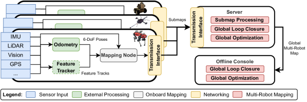
The general structure of the maplab 2.0 framework is presented in Figure 2. The entire framework can be divided into three main components: the mapping node, the mapping server, and the offline console interface. We begin with an overview of the underlying map structure in maplab 2.0, after which we discuss in more detail the main components.
III-A Map Structure
We denote a map as a collection of one or more missions, where each mission is based on a single continuous mapping session. The underlying structure of a map is a factor graph consisting of vertices and edges that incorporate all the robot information and the measurements across different missions. The state of the robot at a certain point in time is parameterized as a vertex (6 degrees of freedom (DoF) pose, velocity, IMU biases). Landmarks are also represented as vertices in the graph whose state is defined as a 3D position. The 3D landmarks can be used as an underlying representation for anything in the environment with a 3D position, e.g., visual landmarks, 3D landmarks, or even semantic objects.
III-A1 Constraints
Vertices are connected through different types of edges that impose constraints on their state variables based on observations (e.g., keypoints, imu measurements, and loop closures). IMU edges contain the pre-integrated IMU measurements between connected vertices and therefore only connect temporally sequential vertices. Relative pose constraint edges impose a rigid 6 DoF transformation between two vertices and are used to represent either relative motion (i.e., odometry) or loop closures across larger temporal gaps or missions. The edges are assigned a covariance to quantify the measurement noise, which is typically set to a predefined constant value. The covariance can be used to model the degrees of motion a sensor can observe, e.g. wheel odometry has infinite covariance for motion along the z-axis, as well as pitch and roll. We consider loop closure edges a special case of relative pose constraint edges. For increased robustness and to account for outliers, loop closure edges can be included as switchable constraints [22]. The optimizer can then discard edges from the graph if they conflict too much with the other constraints. Finally, edges connect a landmark to the poses from which it was observed and impose an error based on the difference between the estimated and observed landmark position.
During optimization, constraints can also be imposed directly on the internal states of chosen vertices. For example, absolute constraints enforce a global 3D position on a vertex with a given uncertainty and allow us to integrate GPS measurements or absolute fiducial marker observations. Additionally, fixing certain states enables the flexibility of choosing which parts of the problem are to be optimized.
III-A2 Landmarks
The visual mapping module at the core of maplab [11] is still a part of maplab 2.0. It includes feature detection based on ORB [23], with binary descriptors from either BRISK [24] or FREAK [25]. Feature correspondences between consecutive frames are established based on descriptor matches, where for robustness, the matching window is restricted by integrated gyroscope measurements. These feature tracks are then triangulated into 3D landmarks.
Global localization and loop closure is done by taking individual frames and establishing a set of 2D-3D matches using the feature descriptors. A covisibility check is applied afterward to the matches to filter outliers. Then, with a P3P algorithm within a RANSAC scheme, the remaining matches are used to obtain a transformation with respect to the map’s reference frame. This transformation can then be added to the factor graph as a loop closure edge. We also provide an alternative method that incorporates loop closures by merging the covisible landmarks and minimizing their reprojection error. This approach foregoes the difficulty of tuning explicit loop closure edge covariances but enforces softer constraints on the factor graph.
In maplab 2.0, we have added the possibility of concurrently including any number of different types of features into the map. To obtain feature tracks across consecutive frames, users can either use the included generic implementation of a Lucas–Kanade tracker [26] or supply the track information themselves. In addition, we expanded the matching engine to support floating point descriptors, enabling loop closure using the latest developed descriptors. Binary descriptors are matched, as in maplab, using an inverted multi-index [27], while floating point descriptors are matched using a Fast Library for Approximate Nearest Neighbors (FLANN) [28]. Matches are then treated similarly for the purpose of loop closures as previously described. Still, for tuning purposes, different feature types can have separate parameter sets to account for differences in quality and behavior.
maplab 2.0 can also handle landmarks with 3D observations. These could originate from, for example, RGB-D cameras, where visual features also have an associated depth, or from features detected directly in a 3D point cloud. The significant difference is that the position of these landmarks is not triangulated using multi-view geometry but by averaging the 3D measurements. Similarly, the pose graph error term is not based on the reprojection error, but on the Euclidean distance between the observed 3D position and the 3D position of the landmark. The other significant difference is that loop closure is set up as a 3D to 3D RANSAC matching problem without the P3P algorithm.
III-B Mapping Node
The mapping node runs onboard each robot and uses external input sources and the raw sensor data to create a map in the form of a multi-modal factor graph. A 6 DoF odometry input is used during map building to initialize the robot pose vertices for the underlying factor graph. The mapping node is agnostic to the odometry method and features a simple interface, thus enabling its easy use across various robots and sensor setups. This is in contrast to maplab [11], where only the built-in visual-inertial estimator ROVIOLI [29] was available – whereas maplab 2.0 does not even require an IMU. However, if an IMU is available, inertial constraints are added to the map, and the state estimator can optionally also compute an initial estimate for the IMU biases. These bias estimates can then be used to improve the initialization of the global map optimization problem, which benefits its convergence speed and accuracy. If an IMU is present but not used by the state estimator, the bias estimation can also be done separately [30, 31, 32].
Substantial changes to the original maplab framework were also made such that other sensor modalities can be processed and integrated using custom internal components or easily configurable external interfaces. Most notably, maplab 2.0 can incorporate any number of different 3D landmarks types at runtime. Furthermore, relative constraints (e.g., odometry or external loop closures) and absolute 6 DoF constraints (e.g., GPS or fiducial markers) can now seamlessly be added.
The raw camera images or the LiDAR point clouds can be attached to the map as resources that later modules can use at any time, for example, to compute additional loop-closures or detect objects. The resulting maps with all the included constraints can then be passed on to the mapping server for online processing or stored and loaded for later offline processing in the console.

III-C Mapping Server
The mapping server is a new addition to maplab 2.0, enabling collaborative and online mapping. This method was successfully deployed in the DARPA Subterranean Challenge as part of the winning team’s (CERBERUS) multi-robot mapping system [33]. The server node can run on a dedicated machine or one of the robots in parallel with the mapping node. The mapping nodes divide their maps into chunks, called submaps, at regular intervals. The submaps are immediately transmitted to the mapping server where they are preprocessed and concatenated to the corresponding previously transmitted submap from the same robot. Bookkeeping is done by duplicating the last vertex of each submap into the next submap when splitting. This also avoids discontinuities in edges and feature tracks. In parallel the server continuously loop closes maps from different robots into a globally consistent map. Notably, the server and console share the same code base, therefore any new functionalities can easily be integrated into either one.
III-C1 Submap Preprocessing
The incoming submaps are not merged directly but rather first processed individually to ensure local accuracy. Specifically, a configurable set of operations is executed on each robot’s submap, which includes local map optimization (full bundle adjustment over all sensor data and constraints), feature quality evaluation, and intra-map loop closure (visual and LiDAR depending on what is available). Since the submaps are processed independently of each other, the mapping server can efficiently process multiple maps concurrently. After completion of the preprocessing steps, each finished submap is concatenated to the previous submap from the same robot.
III-C2 Multi-Robot Processing
The mapping server continuously operates on the global multi-robot map and executes a second set of configurable operations (loop closure, feature quality evaluation, bundle adjustment, visualizations, absolute constraint outlier rejection, etc.). Here, the loop closure algorithms (visual or LiDAR) try and place all the different robots into the same reference frame and correct drift. In contrast to the preprocessing step, the operations on the multi-robot map are always performed at a global scope, e.g., loop closures are detected in an intra- and inter-robot approach, and the global optimization is done jointly over all robot maps. The collaboratively built global map can also be transmitted back to the robots to increase the accuracy of their onboard estimation [13]. The increased awareness of the environment not only benefits localization accuracy but also other tasks such as global path planning.
III-D Offline Console
The offline console was ported over from maplab, with old tools adapted to the new features regarding sensors and modalities. There are tools for further processing maps, such as batch optimization, merging maps from different sessions, outlier rejection, key-framing, map sparsification [34], etc. Loop closure using LiDAR is also now possible with a new module that includes an implementation of ICP [35] and G-ICP [36] but is not limited to these and can easily be extended. Transformations computed by the registration module are added as loop closure edges with switchable constraints (see Section III-A). For each sensor and method combination we use a predefined fixed covariance, which is set separately for each translation and rotation component. The values are empirically chosen based on the sensor noise and the accuracy of the registration method. Dense reconstruction can also be done using the integrated Voxblox [37] plugin. The console additionally provides tools for resource management (manipulating or visualizing the attached point clouds, images, and semantic measurements) or exporting map data (poses, IMU biases, landmarks, etc.).
Finally, the console enables easy extensions through plugins that can run code offline and are independent of the map-building process. We used plugins, for example, to implement the LiDAR registration module mentioned above and a semantic loop closure module (see Section IV-D).
IV Use-Cases
We conducted several experiments to evaluate our proposed framework thoroughly and to demonstrate its ease of use and high flexibility. Specifically, this section presents results on four datasets to showcase the new features and capabilities of maplab 2.0. First, we validate the performance and accuracy of our proposed framework on the public HILTI SLAM 2021 dataset [38] and compare it to well-known state-of-the-art approaches. Next, we demonstrate the real-world applicability of our proposed framework and showcase the large-scale multi-robot multi-session capabilities. Then, we show the versatility of the landmark system by incorporating 3D LiDAR features detected from projected point clouds. Finally, we showcase a semantic loop closure module on a custom indoor dataset. All datasets are collected with hardware time-synchronized sensor setups.
IV-A Validation and Comparison
We use the HILTI SLAM Challenge 2021 dataset [38] to compare our proposed framework to state-of-the-art approaches. The dataset includes 12 recordings covering indoor office environments and challenging outdoor construction sites. In our experiments we exclude three sequences that are too small and do not present interesting challenges. Three pairs (Construction Site, Basement, and Campus) of the remaining nine sequences were taken in the same environment and can be co-localized to increase accuracy.
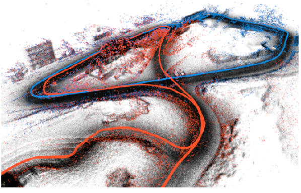
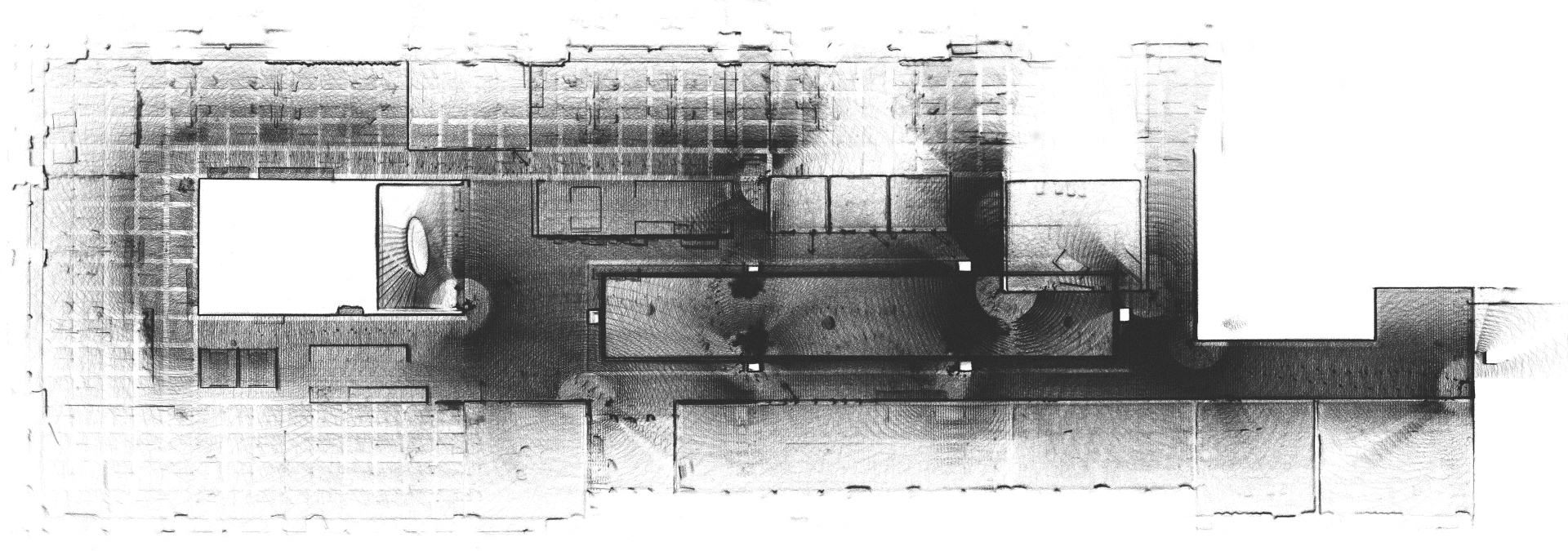
For maplab 2.0, we can use the five cameras, the ADIS IMU and the OS0-64 LiDAR provided in the dataset. We show three use-cases for maplab 2.0 using three different odometry sources: ROVIO [29], OKVIS [39], and FAST-LIO2 [40]. Besides the standard BRISK [24] descriptors, we use the external interfaces from Section III-A2 to also include SuperPoint [12] features with SuperGlue [41] tracking, and SIFT features [42] with LK tracking [26]. To reduce map size and speed up the descriptor search, we compress the SuperPoint and SIFT features using principal component analysis (PCA) from floating points to . Global loop closures are computed using all available features, and matched landmarks are merged. We also use ICP [35] from the LiDAR registration module (see Section III-D) to refine our poses locally. Covariances for the loop closure edges are predefined empirically. Visualizations from sequence Office Mitte are presented in Figure 3a-c. It can be observed how SuperPoint features better follow the building structure compared to ORB.
| HILTI 2021 SLAM Dataset | |||||||||||
| Sequence | maplab 2.0 | ||||||||||
| ORB | LVI | RTAB | maplab | ROVIO | OKVIS | FAST | ROVIO | OKVIS | FAST-LIO2 | ||
| SLAM3 | SAM | Map | LIO2 | + SIFT | + SP + B | + ICP | + SP + B | ||||
|
|
|
|
|
|
|
|
|
|
|
|
|
| Construction 1 | 1.55 | 0.13 | 0.36 | 0.16 | 0.98 | 1.17 | 0.04 | 0.14 | 0.08 | 0.08 | 0.04 |
| Construction 2 | 2.77 | 0.33 | 0.67 | 0.57 | 1.50 | 2.13 | 0.07 | 0.34 | 0.19 | 0.19 | 0.07 |
| IC Office | 1.86 | 0.12 | 1.50 | 0.09 | 1.16 | 1.27 | 0.08 | 0.08 | 0.08 | 0.07 | 0.07 |
| Office Mitte | 1.70 | 0.24 | 0.94 | 3.18 | 0.86 | 1.15 | 0.12 | 0.27 | 0.18 | 0.15 | 0.10 |
| Basement 3 | 1.55 | 0.10 | 0.38 | 0.09 | 3.05 | 1.01 | 0.05 | 0.09 | 0.09 | 0.08 | 0.05 |
| Basement 4 | 1.71 | 0.13 | 0.38 | 0.11 | 2.90 | 1.23 | 0.04 | 0.11 | 0.10 | 0.09 | 0.04 |
| Parking | 5.49 | 4.43 | 7.82 | 0.39 | 6.13 | 3.36 | 5.00 | 0.31 | 0.21 | 0.21 | 0.21 |
| Campus 1 | 1.93 | 0.12 | 0.93 | 0.60 | 5.10 | 2.41 | 0.07 | 0.38 | 0.19 | 0.17 | 0.07 |
| Campus 2 | 2.24 | 0.14 | 0.79 | 0.47 | 2.02 | 2.23 | 0.09 | 0.28 | 0.20 | 0.18 | 0.08 |
| Total Time | 61 | 68 | 163 | 82 | 58 | 121 | 52 | 98 | 236 | 267 | 194 |
Table II also shows the performance of the odometry sources alone, and other SLAM baselines (LVI-SAM [43], ORB-SLAM3 [8], RTAB-Map [3], and maplab [11]). Maplab and maplab 2.0 are the only methods able to use all five cameras for loop closures. For ROVIO and OKVIS we only use the frontal camera or stereo pair for odometry. Among all methods that use vision maplab 2.0 outperforms the baselines by a significant margin. FAST-LIO2, which uses only LiDAR-Inertial, is the best baseline, outperforming even LVI-SAM, which is a vision-LiDAR-inertial fusion based on the same principles. However, we show that we can also take the best performing method as odometry and further refine the result, especially improving significantly on the Parking sequence over FAST-LIO2. We also present a fusion of ROVIO and SIFT, demonstrating the versatility of maplab 2.0 for fast incremental improvements, independently of better deep-learned visual features. Timings for all methods are also presented on a machine with an Intel i7-8700 and an Nvidia RTX 2080 GPU.
IV-B Large-Scale Multi-Robot Multi-Session Mapping
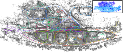
We demonstrate the applicability toward complex real-world scenarios by deploying our proposed framework in a large-scale training facility in Switzerland. The environment features urban-like streets with buildings and harsh environments such as collapsed buildings with narrow spaces. For this experiment, we recorded 23 individual runs with a handheld device with five cameras and an Ouster OS0-128 comprising more than two hours of data over approximately and multiple indoors-outdoors transitions. Each run used OKVIS [39] for odometry. The first five maps were used to build a global multi-robot map using the mapping server, and the remaining maps were merged using multi-session mapping in the console. Consistency between all missions was enforced using global visual loop closures, and if available, additional absolute pose constraints from an RTK GPS. Moreover, individual trajectories were refined by performing intra- and inter-mission LiDAR registrations. Figure 4 shows the final multi-robot map.
To quantitatively evaluate the multi-robot server we test on the public EuRoC benchmark [44]. As the console and server use the same underlying mapping framework, excluding minor details such as operation ordering, the expected accuracy is the same. We run all 11 sequences simultaneously in a multi-robot experiment using the mapping server, with ROVIO and BRISK. Afterwards, we repeat the experiment by sequentially processing each mission using the mapping node and console and then merging them together. Both scenarios achieve an average RMSE APE of 0.043 , but the parallelized mapping server only takes 3 27 for everything, as opposed to 35 56 for the sequential multi-session workflow. For both scenarios the timings include the odometry, optimization and map merging.
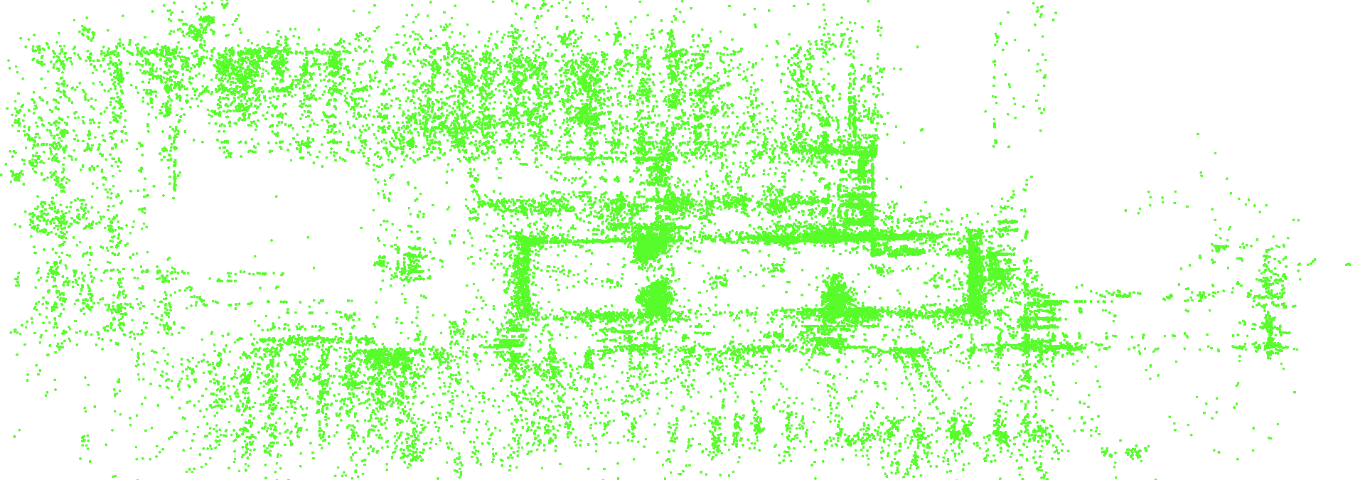
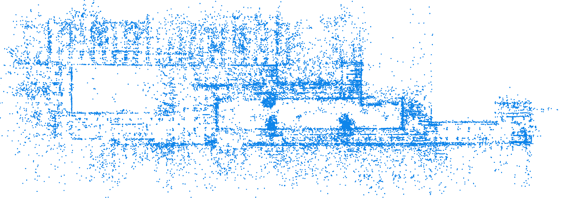
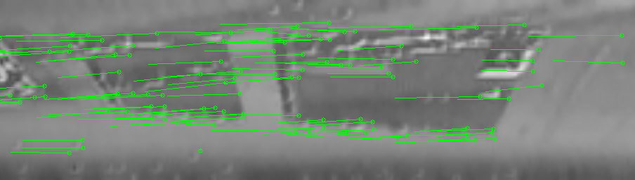
IV-C Visual Tracking on Projected LiDAR Images
To showcase the flexibility of the landmark system in maplab 2.0, we integrate 3D LiDAR keypoints111Please note that a similar workflow could be implemented for other modalities, e.g., RGB-D cameras, radar or sonar imaging.. We draw inspiration from the work of Streiff et al. [45] and project the LiDAR point cloud onto a 2D plane. We normalize the LiDAR range and intensity values using a logarithmic scale and merge the two channels using Mertens fusion [46]. Missing pixels from bad LiDAR returns are in-painted using neighboring values. An example image of the resulting 2D projection is shown in Figure 5, alongside a camera image from the same perspective showing the environment. We then treat the LiDAR image like a camera image and apply SuperPoint with SuperGlue to obtain point features and tracks, as shown in Figure 5. Since, for each feature observation, we have depth information from the LiDAR, we can more efficiently initialize and loop close these 3D LiDAR landmarks, as described in Section III-A2. Finally, we use these LiDAR keypoints to map out one of the sequences in the HILTI 2021 dataset and visualize the resulting map in Figure 3(d). The LiDAR landmarks are mapped more accurately onto the structure than the visual keypoints, as seen from the straightness of the walls. However, they also suffer from outliers caused by noise in the LiDAR image from missing points or moving objects in the environment.
IV-D Semantic-based Mapping
This section showcases the extensibility and modular design of maplab 2.0 by augmenting the map with semantic information and illustrating its potential application in a real-world scenario. Initially, semantic objects are detected in an image using Mask R-CNN [47], and for each detection, we use NetVLAD [48] to extract a descriptor on the masked instance segmentation. Instead of the built-in tracker, all detected objects are tracked using Deep SORT [49], which extends typical spatial data association metrics with an appearance term that can directly utilize the previously extracted object descriptor. Similar to visual landmarks, semantic objects are 3D landmarks in the maplab 2.0 map but have an associated class label and can be used for, e.g., semantic loop closure detection.
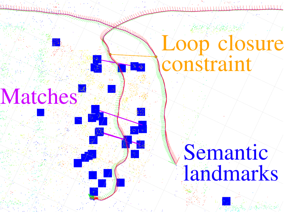
Finally, candidate semantic loop closures are found by directly comparing the object descriptors of the same class. First, a unique visibility filter is applied, i.e., two landmarks observed in a single image cannot be matched. After geometrically verifying the candidates and clustering co-visible landmarks, a 6-DoF constraint between the two robot vertices closest to two matched landmark clusters is constructed using the relative coordinate transformation between two 3D landmark clusters, obtained through Horn’s method [50]. Finally, the covariance of the corresponding factor-graph constraint is calculated using the method proposed by Manoj et al. [51].
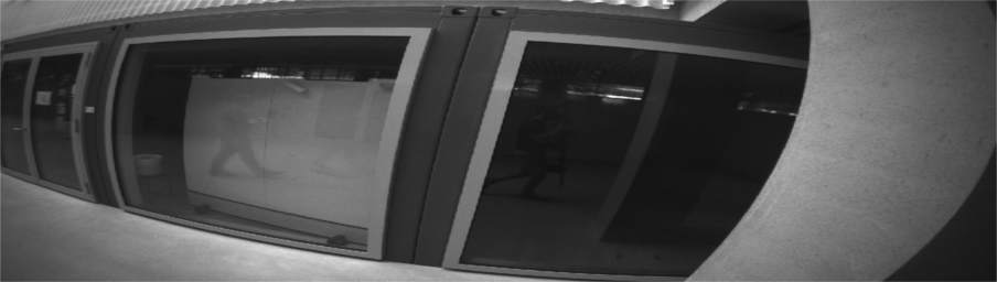
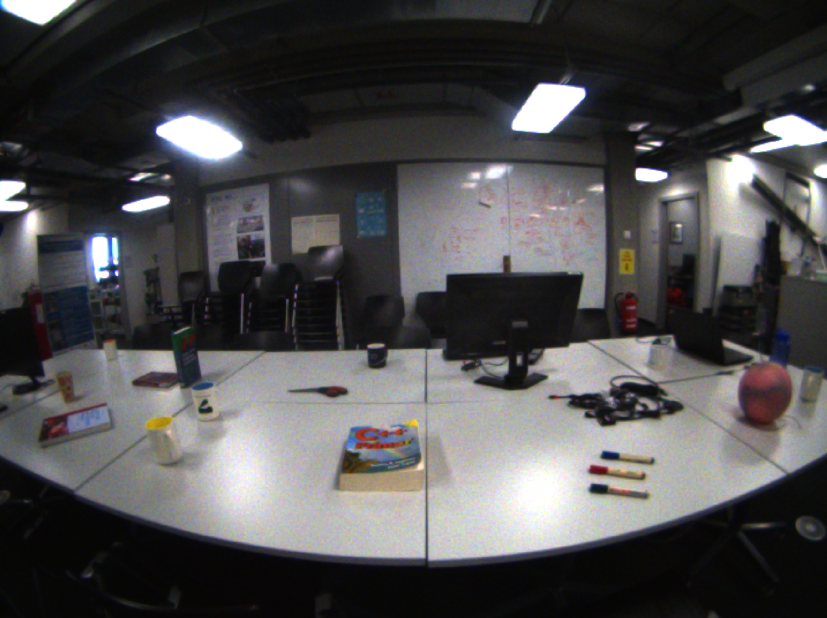
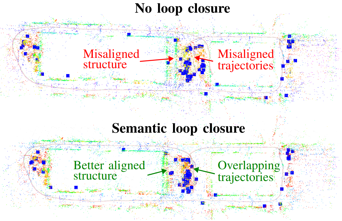
We collected an indoor dataset in an office environment with multiple objects using an RGB-inertial sensor [52]. We observe an office table with objects on two occasions while leaving some time to accumulate drift (see Figure 6(a) and 6(c)). Figure 6(b) shows semantic landmark clusters and detected loop closure candidates. After adding the loop closure edges from the semantic objects to the full factor graph, the drift significantly reduces, and an improved map can be seen in Figure 6(c).
V Conclusion
We presented a research platform for multi-modal and multi-robot mapping, supporting online and offline processing of the maps. We showcase state-of-the-art performance on a large-scale SLAM benchmark and multiple experimental use cases for maplab 2.0. Our proposed mapping framework’s flexible and modular design facilitates research in various robotic applications and yields important implications in academia and industry. The code and tutorials to reproduce the experiments are available on the wiki of the repository.
- FLANN
- Fast Library for Approximate Nearest Neighbors
- ADAS
- advanced driving assistance systems
- AE
- auto-exposure
- ASL
- Autonomous Systems Lab
- BA
- bundle adjustment
- BM
- block-matching
- BoW
- Bag-of-Words
- BRISK
- Binary Rotation Invariant Scalable Keypoint
- CLAHE
- contrast limiting adaptive histogram equalization
- CNN
- Convolutional Neural Network
- CPU
- central processing unit
- DAVIS
- Dynamic and Active Vision Sensor
- DCNN
- Deep Convolutional Neural Network
- DL
- deep learning
- DoF
- degrees of freedom
- DSO
- Direct Sparse Odometry
- DVS
- Dynamic Vision Sensor
- EKF
- extended Kalman filter
- ETCS
- European Train Control System
- ETSC
- European Train Security Council
- ESDF
- Euclidean signed distance field
- FAST
- Features form Accelerated Segment Test
- FC
- fully connected
- FIR
- finite impulse response
- FoV
- field of view
- FPGA
- field-programmable gate array
- FPS
- frames per second
- GNSS
- global navigation satellite system
- GP
- Gaussian Process
- GPM
- Gaussian preintegrated measurement
- GPS
- Global Positioning System
- GPU
- graphics processing unit
- GT
- ground truth
- GTC
- ground truth clustering
- GTSAM
- Georgia Tech Smoothing and Mapping library
- HDR
- High Dynamic Range
- HS
- Hough space
- HT
- Hough transform
- I2C
- Inter-Integrated Circuit
- IDOL
- IMU-DVS Odometry with Lines
- IMU
- inertial measurement unit
- INS
- inertial navigation system
- IOU
- intersection over union
- KF
- Kalman filter
- LED
- light emitting diode
- LiDAR
- Light Detection and Ranging sensor
- LSD
- line segment detector
- LSSVM
- least squares support vector machine
- LWIR
- long-wave infrared
- MAV
- micro aerial vehicle
- MCU
- micro controller unit
- NCLT
- North Campus Long-Term
- NMI
- normalized mutual information
- NMS
- non-maxima suppression
- NN
- nearest neighbor
- OS
- operating system
- PCB
- printed circuit board
- PC
- point cloud
- PCA
- principal component analysis
- PCM
- probabilistic curvemap
- PF
- particle filter
- PPS
- Pulse per second
- PTP
- Precision Time Protocol
- RANSAC
- random sample consensus
- RGB-D-I
- Color-Depth-Inertial
- R-IOU
- reprojection intersection over union
- RMSE
- root mean square error
- RNN
- recurrent neural network
- ROI
- region of interest
- ROS
- Robot Operating System
- RQE
- Rényi’s Quadric Entropy
- RTK
- real time kinematics
- SBB
- Schweizerische Bundesbahnen
- SIFT
- Scale Invariant Feature Transform
- SLAM
- Simultaneous Localization And Mapping
- SNN
- spiking neural network
- SNR
- signal to noise ratio
- SP
- SuperPoint
- SPI
- Serial Peripheral Interface
- SQ
- superquadric
- SWE
- Sliding Window Estimator
- ToF
- time of flight
- TSDF
- Truncated Signed Distance Function
- TUM
- Technische Universität München
- UART
- Universal Asynchronous Receiver Transmitter
- UAV
- unmanned aerial vehicle
- USB
- universal serial bus
- VBG
- Verkehrsbetriebe Glattal AG
- VBZ
- Verkehrsbetriebe Zürich
- VersaVIS
- Open Versatile Multi-Camera Visual-Inertial Sensor Suite
- VI
- visual-inertial
- VIO
- visual-inertial odometry
- VO
- visual odometry
- ZVV
- Zürich Verkehrsverein
- SVD
- Singular Value Decomposition
- DLT
- Direct Linear Transform
- UGV
- unmanned ground vehicle
- AR
- augmented reality
- VR
- virtual reality
- ATO
- autonomous train operation
- APE
- absolute position error
References
- [1] G. Bresson, Z. Alsayed, L. Yu, and S. Glaser, “Simultaneous localization and mapping: A survey of current trends in autonomous driving,” T-IV, vol. 2, no. 3, pp. 194–220, 2017.
- [2] K. Blomqvist, M. Breyer, A. Cramariuc, J. Förster, M. Grinvald, F. Tschopp, J. J. Chung, L. Ott, J. Nieto, and R. Siegwart, “Go Fetch: Mobile Manipulation in Unstructured Environments,” in Workshop on Perception, Action, Learning, ICRA, 2020.
- [3] M. Labbé and F. Michaud, “RTAB-Map as an open-source lidar and visual simultaneous localization and mapping library for large-scale and long-term online operation,” JFR, vol. 36, no. 2, pp. 416–446, 2019.
- [4] A. Rosinol, M. Abate, Y. Chang, and L. Carlone, “Kimera: An Open-Source Library for Real-Time Metric-Semantic Localization and Mapping,” in ICRA, 5 2020, pp. 1689–1696.
- [5] Y. Tian, Y. Chang, F. Herrera Arias, C. Nieto-Granda, J. How, and L. Carlone, “Kimera-Multi: Robust, Distributed, Dense Metric-Semantic SLAM for Multi-Robot Systems,” T-RO, pp. 1–17, 2022.
- [6] Y. Chang, K. Ebadi, C. E. Denniston, M. F. Ginting, A. Rosinol, A. Reinke, M. Palieri, J. Shi, A. Chatterjee, B. Morrell, et al., “LAMP 2.0: A Robust Multi-Robot SLAM System for Operation in Challenging Large-Scale Underground Environments,” RA-L, 2022.
- [7] M. Karrer, P. Schmuck, and M. Chli, “CVI-SLAM—collaborative visual-inertial SLAM,” RA-L, vol. 3, no. 4, pp. 2762–2769, 2018.
- [8] C. Campos, R. Elvira, J. J. G. Rodríguez, J. M. Montiel, and J. D. Tardós, “ORB-SLAM3: An Accurate Open-Source Library for Visual, Visual–Inertial, and Multimap SLAM,” T-RO, 2021.
- [9] P. Schmuck, T. Ziegler, M. Karrer, J. Perraudin, and M. Chli, “COVINS: Visual-Inertial SLAM for Centralized Collaboration,” in ISMAR-Adjunct, 2021, pp. 171–176.
- [10] P.-Y. Lajoie, B. Ramtoula, Y. Chang, L. Carlone, and G. Beltrame, “DOOR-SLAM: Distributed, online, and outlier resilient SLAM for robotic teams,” RA-L, vol. 5, no. 2, pp. 1656–1663, 2020.
- [11] T. Schneider, M. Dymczyk, M. Fehr, K. Egger, S. Lynen, I. Gilitschenski, and R. Siegwart, “maplab: An Open Framework for Research in Visual-inertial Mapping and Localization,” RA-L, vol. 3, no. 3, pp. 1418–1425, 11 2018.
- [12] D. Detone, T. Malisiewicz, and A. Rabinovich, “SuperPoint: Self-supervised interest point detection and description,” in CVPR Workshops, 12 2018, pp. 337–349.
- [13] L. Bernreiter, S. Khattak, L. Ott, R. Siegwart, M. Hutter, and C. Cadena, “Collaborative robot mapping using spectral graph analysis,” in ICRA, 2022.
- [14] C. Cadena, L. Carlone, H. Carrillo, Y. Latif, D. Scaramuzza, J. Neira, I. Reid, and J. J. Leonard, “Past, present, and future of simultaneous localization and mapping: Toward the robust-perception age,” T-RO., vol. 32, no. 6, pp. 1309–1332, 2016.
- [15] R. Mur-Artal and J. D. Tardos, “ORB-SLAM2: An Open-Source SLAM System for Monocular, Stereo, and RGB-D Cameras,” T-RO, pp. 1–8, 2017.
- [16] M. Labbé and F. Michaud, “Multi-Session Visual SLAM for Illumination-Invariant Re-Localization in Indoor Environments,” Frontiers in Robotics and AI, p. 115, 2022.
- [17] R. Dubé, A. Cramariuc, D. Dugas, H. Sommer, M. Dymczyk, J. Nieto, R. Siegwart, and C. Cadena, “SegMap: Segment-based mapping and localization using data-driven descriptors,” IJRR, vol. 39, no. 2-3, pp. 339–355, 2020.
- [18] A. Gawel, C. Del Don, R. Siegwart, J. Nieto, and C. Cadena, “X-View: Graph-Based Semantic Multi-View Localization,” RA-L, vol. 3, no. 3, pp. 1687–1694, 2017.
- [19] A. Cramariuc, F. Tschopp, N. Alatur, S. Benz, T. Falck, M. Brühlmeier, B. Hahn, J. Nieto, and R. Siegwart, “SemSegMap – 3D Segment-based Semantic Localization,” IROS, 2021.
- [20] F. Taubner, F. Tschopp, T. Novkovic, R. Siegwart, and F. Furrer, “LCD - Line Clustering and Description for Place Recognition,” in 3DV, 2020, pp. 908–917.
- [21] L. Bernreiter, A. Gawel, H. Sommer, J. Nieto, R. Siegwart, and C. Cadena, “Multiple hypothesis semantic mapping for robust data association,” RA-L, vol. 4, no. 4, pp. 3255–3262, 2019.
- [22] N. Sünderhauf and P. Protzel, “Switchable constraints for robust pose graph SLAM,” in IROS, 2012, pp. 1879–1884.
- [23] E. Rublee, V. Rabaud, K. Konolige, and G. Bradski, “ORB: An efficient alternative to SIFT or SURF,” in ICCV, 2011, pp. 2564–2571.
- [24] S. Leutenegger, M. M. Chli, and R. Y. Siegwart, “Binary Robust Invariant Scalable Keypoints,” in ICCV, 2011, pp. 2548–2555.
- [25] A. Alahi, R. Ortiz, and P. Vandergheynst, “FREAK: Fast Retina Keypoint,” in CVPR, 2012, pp. 510–517.
- [26] B. D. Lucas and T. Kanade, “An Iterative Image Registration Technique with an Application to Stereo Vision,” Imaging, vol. 130, pp. 674–679, 1981.
- [27] S. Lynen, T. Sattler, M. Bosse, J. Hesch, M. Pollefeys, and R. Siegwart, “Get Out of My Lab: Large-scale, Real-Time Visual-Inertial Localization,” in RSS, 2015, p. 18.
- [28] M. Muja and D. G. Lowe, “Fast approximate nearest neighbors with automatic algorithm configuration.” VISAPP, vol. 2, no. 331-340, p. 2, 2009.
- [29] M. Bloesch, M. Burri, S. Omari, M. Hutter, and R. Siegwart, “Iterated extended Kalman filter based visual-inertial odometry using direct photometric feedback,” IJRR, vol. 36, no. 10, pp. 1053–1072, 2017.
- [30] S. Lynen, M. W. Achtelik, S. Weiss, M. Chli, and R. Siegwart, “A robust and modular multi-sensor fusion approach applied to MAV navigation,” in IROS, 2013, pp. 3923–3929.
- [31] S. O. Madgwick, A. J. Harrison, and R. Vaidyanathan, “Estimation of IMU and MARG orientation using a gradient descent algorithm,” ICORR, 2011.
- [32] R. G. Valenti, I. Dryanovski, and J. Xiao, “Keeping a good attitude: A quaternion-based orientation filter for IMUs and MARGs,” Sensors, vol. 15, no. 8, pp. 19 302–19 330, 2015.
- [33] M. Tranzatto, T. Miki, M. Dharmadhikari, L. Bernreiter, M. Kulkarni, F. Mascarich, O. Andersson, S. Khattak, M. Hutter, R. Siegwart, and K. Alexis, “CERBERUS in the DARPA Subterranean Challenge,” Science Robotics, vol. 7, no. 66, 2022.
- [34] M. Dymczyk, S. Lynen, T. Cieslewski, M. Bosse, R. Siegwart, and P. Furgale, “The gist of maps - Summarizing experience for lifelong localization,” in ICRA, 2015, pp. 2767–2773.
- [35] F. Pomerleau, F. Colas, R. Siegwart, and S. Magnenat, “Comparing ICP variants on real-world data sets Open-source library and experimental protocol,” Autonomous Robots, vol. 34, no. 3, 2014.
- [36] A. Segal, D. Haehnel, and S. Thrun, “Generalized-ICP,” in Robotics: Science and Systems, vol. 2, no. 4, 2009, p. 435.
- [37] H. Oleynikova, Z. Taylor, M. Fehr, R. Siegwart, and J. Nieto, “Voxblox: Incremental 3D Euclidean Signed Distance Fields for on-board MAV planning,” in IROS, 2017, pp. 1366–1373.
- [38] M. Helmberger, K. Morin, B. Berner, N. Kumar, G. Cioffi, and D. Scaramuzza, “The hilti slam challenge dataset,” RA-L, 2022.
- [39] S. Leutenegger, S. Lynen, M. Bosse, R. Siegwart, and P. Furgale, “Keyframe-based visual-inertial odometry using nonlinear optimization,” IJRR, vol. 34, no. 3, pp. 314–334, 2015.
- [40] W. Xu, Y. Cai, D. He, J. Lin, and F. Zhang, “FAST-LIO2: Fast Direct LiDAR-Inertial Odometry,” T-RO, vol. 38, no. 4, pp. 2053–2073, 2022.
- [41] P.-E. Sarlin, D. DeTone, T. Malisiewicz, and A. Rabinovich, “SuperGlue: Learning Feature Matching with Graph Neural Networks,” in PCVPR, 2020, pp. 4938–4947.
- [42] D. G. Lowe, “Object recognition from local scale-invariant features,” in ICCV, vol. 2, 1999, pp. 1150–1157.
- [43] T. Shan, B. Englot, C. Ratti, and D. Rus, “LVI-SAM: Tightly-coupled Lidar-Visual-Inertial Odometry via Smoothing and Mapping,” in ICRA, 2021, pp. 5692–5698.
- [44] M. Burri, J. Nikolic, P. Gohl, T. Schneider, J. Rehder, S. Omari, M. W. Achtelik, and R. Siegwart, “The EuRoC micro aerial vehicle datasets,” IJRR, vol. 35, no. 10, pp. 1157–1163, 2016.
- [45] D. Streiff, L. Bernreiter, F. Tschopp, M. Fehr, and R. Siegwart, “3D3L: Deep Learned 3D Keypoint Detection and Description for LiDARs,” in ICRA. IEEE, 2021, pp. 13 064–13 070.
- [46] T. Mertens, J. Kautz, and F. Van Reeth, “Exposure fusion,” in Pacific Graphics. IEEE, 2007, pp. 382–390.
- [47] K. He, G. Gkioxari, P. Dollar, and R. Girshick, “Mask R-CNN,” in ICCV, 2017, pp. 2980–2988.
- [48] R. Arandjelovic, P. Gronat, A. Torii, T. Pajdla, and J. Sivic, “NetVLAD: CNN Architecture for Weakly Supervised Place Recognition,” PAMI, vol. 40, no. 6, pp. 1437–1451, 6 2018.
- [49] N. Wojke, A. Bewley, and D. Paulus, “Simple Online and Realtime Tracking with a Deep Association Metric,” in ICIP, 2017, pp. 3645–3649.
- [50] B. K. Horn, “Closed-form solution of absolute orientation using unit quaternions,” JOSA A, vol. 4, no. 4, pp. 629–642, 1987.
- [51] P. S. Manoj, L. Bingbing, Y. Rui, and W. Lin, “A Closed-form Estimate of 3D ICP Covariance,” in MVA, Tokyo, Japan, 2015.
- [52] F. Tschopp, M. Riner, M. Fehr, L. Bernreiter, F. Furrer, T. Novkovic, A. Pfrunder, C. Cadena, R. Siegwart, and J. Nieto, “VersaVIS—An Open Versatile Multi-Camera Visual-Inertial Sensor Suite,” Sensors, vol. 20, no. 5, p. 1439, 3 2020.