Thermodynamics of quantum information in noisy polarizers
Abstract
Among the emerging technologies with prophesied quantum advantage, quantum communications has already led to fascinating demonstrations—including quantum teleportation to and from satellites. However, all optical communication necessitates the use of optical devices, and their comprehensive quantum thermodynamic description is still severely lacking. In the present analysis we prove several versions of Landauer’s principle for noisy polarizers, namely absorbing linear polarizers and polarizing beamsplitters. As main results we obtain statements of the second law quantifying the minimal amount of heat that is dissipated in the creating of linearly polarized light. Our findings are illustrated with an experimentally tractable example, namely the temperature dependence of a quantum eraser.
I Introduction
There are generally three applications in which quantum advantage is expected to be of technological significance—computation, sensing, and communication [1]. Despite the distinct and unique technological challenges of each area, devices designed for each of these applications can be considered quantum devices that process information. Hence, they can be described by means of quantum thermodynamics [2].
The development of classical thermodynamics of information [3] originated in the formulation of Landauer’s principle [4]. This statement of the second law asserts that any computational task requiring the erasure of information must result in dissipation of heat, and the amount of heat produced is at least times the number of logical bits erased. Recent years have seen intense research efforts in generalizing the bound to a wide variety of physical situations, such as classical systems with both discrete and continuous state spaces [5, 6, 7, 8, 9], as well as quantum systems undergoing Markovian and non-Markovian dynamics [10, 11, 12, 13]. Landauer’s principle has even been experimentally verified in microscale systems using an overdamped colloidal particle in a double-well potential [14]. However, given the rather heuristic nature of the original formulation [4], it is still being debated whether the original statement can really be shown in all generality [15, 16, 17]. Notably, some authors have recently interpreted certain non-Markovian processes as violations of Landauer’s principle [18, 19, 20, 21, 22].
Curiously, most of the current discussion is focused on statements of Landauer’s principle for computation. Yet, the communication of quantum information also obviously incurs thermodynamic costs, which can be determined with versions of the Landauer bound. Such “dynamical” formulations of Landauer’s principle can be traced back to Bremermann [23], who proposed that any computational device must obey the fundamental laws of physics namely special relativity, quantum mechanics, and thermodynamics. Then, identifying Shannon’s noise energy with the in Heisenberg’s uncertainty relation [24] for energy and time, , he found an upper bound on the rate with which information can be communicated. A more rigorous argument was put forward by Bekenstein [25] in the context of black hole thermodynamics [26, 27, 28, 29, 30]. However, the Bremermann-Bekenstein bound does not seem to enjoy the same prominence as Landauer’s principle, and in fact many different statements for the maximal rate with which entropy and information can be communicated have been formulated [31, 32, 33, 34, 35, 36, 37, 38, 39, 40, 41, 42, 43, 44].
In the present work, we will be analyzing the thermodynamics of some aspects of quantum optical communication. This is motivated by the fact that light is an attractive physical platform, given that it can carry information at the greatest possible speed and that it interacts relatively weakly with the environment [45, 46]. The most significant technical challenge in creating optical quantum networks is overcoming attenuation [47, 48]. Entanglement swapping schemes can extend the range of quantum communication [49], but the performance of this method is still limited by the amount of dissipation caused by the individual optical components used [50, 51, 52]. Hence, a comprehensive thermodynamic characterization of noisy optical elements appears urgently needed.
Most communication schemes employ linearly polarized light [53]. Such light can be produced by sending unpolarized light through a linear polarizer, which absorbs one component of the electric field and transmits the component perpendicular to it. We will call such optical elements absorbing linear polarizers (ALP). It is also possible to produce linearly polarized light using a polarizing beamsplitter (PBS), which transmits one component of the electric field and reflects the component which is perpendicular to it. While it is clear that some heat must be generated by the ALP, it is less obvious that there is any minimum amount of dissipation which is caused by the PBS [54, 55]. In what follows we will show that both devices in fact are responsible for dissipation of heat when an assumption of locality is made, which can be understood through the concept of modularity dissipation [9]. Most light sources found in nature can be accurately described by the classical laws of electrodynamics, and their description does not benefit from quantization of the field. However, there are engineered sources available which can produce single or entangled pairs of photons on demand, and the results of experiments done with these sources cannot always be explained by classical electrodynamics [56, 57, 58]. In our analysis, we will first address the case of classical light. The “classicality” of light can be characterized in a number of ways, such as by the negativity of the Wigner function [59, 59, 60]. For our purposes, we will consider classical light to be a statistical mixture of approximate coherent states at large photon number. A derivation is given of a version of Landauer’s principle for ALPs acting on classical sources followed by a derivation of a similar result applicable to to PBSs, assuming the reflected light is inaccessible. Then, we will provide insight into more exotic sources with nonclassical behavior. We show that the findings for the PBS acting on classical light can be seen as stemming from local nonconservation of globally conserved quantities, and that an analogous dissipation cost applies to quantum information processing tasks. Having generalized the PBS result to the quantum case, we investigate the ALP acting on quantum sources, and argue that an ALP can be modeled as a collection of PBSs strung together with intervening thermal reservoirs. Using this model we are able to probe the dynamics of the polarization process, rather than just its end result. Interestingly, our model becomes formally equivalent to a repeated interaction scheme (or collision model) which has received attention recently in the field of open quantum systems [61] including in the context of Landauer’s principle [62], and we leverage these existing results to quantify the dissipation which occurs as (possibly nonclassical) light propagates through the ALP. Notably, our analysis reveals a discontinuity in the slope of the energy-entropy curve as temperature approaches zero, which agrees with previous investigations of the random scattering of light [63]. The collision model approach also allows us to describe the dependence of the ALP’s behavior on its temperature, both in terms of optical extinction and decoherence. This permits us to make predictions concerning the relationship between temperature and the signature of entanglement observed in the quantum eraser [64, 65, 66, 67]. We predict that at higher temperatures the observed restoration of interference caused by measurement is suppressed.
II Landauer’s principle for linear polarizers
In the following, we will be deriving various statements of Landauer’s principle. The principle expresses that a decrease in Shannon entropy of an information-bearing degree of freedom is accompanied by the dissipation of heat [4, 68, 5]
| (1) |
where is the differential Shannon entropy [69]
| (2) |
Here, denotes the probability density function (PDF) of a discrete or continuous random variable .
In our case, is the electric field, in which information is encoded. Then, an ALP has the effect of erasing this information stored in one component of the electric field. Therefore, by Landauer’s principle the ALP should be required to dissipate heat. This is in fact the case, and we now provide the corresponding statement of Landauer’s principle.
II.1 Classical absorbing linear polarizer
The ALP transmits horizontally polarized light and absorbs vertically polarized light. Consider a single mode of the electric field of frequency . The vertical component of the electric field is [70]
| (3) |
where the complex amplitude will be considered a random variable with PDF and is an arbitrary constant electric field strength. The distribution is assumed to have finite variance (and therefore finite energy) but is otherwise unspecified. The differential Shannon entropy of is
| (4) |
where the integral is over the entire complex plane. We assume the field decays rapidly outside of some region with volume , and so the ensemble-averaged energy content of the field’s vertical component is
| (5) |
After the light has passed through the polarizer, we assume that the state of the field afterwards is a thermal state, given by the canonical ensemble, , where is the temperature of the polarizer. Although it is well known that this assumption leads to an infinite total energy in the completely classical case when all frequencies are present [71], this does not affect the present argument, which only concerns a single mode of the field. This thermal state has entropy , and so the total erasure is simply the difference
| (6) |
We show in Appendix A that the following statement of Landauer’s principle holds
| (7) |
Expanding about zero for small , we obtain the Landauer bound
| (8) |
Equations (7) and (8) are our first main results, asserting Landauer’s principle for the ALP. The assumption of finite variance of the field was necessary to avoid having a divergent amount of heat dissipated, and similarly it was necessary to assume that the ALP does not perfectly polarize the field (a thermal distribution at temperature remains in the vertical component) to avoid a divergent change in differential entropy. The assumption that all energy is converted to heat is justified on the basis that the ALP is a passive component with no mechanism for storing energy. If there are multiple frequencies in the source, we may treat the amplitude at each frequency as a random variable , and we assume these are not correlated with each other. In this case due to the additivity of the Shannon entropy and the energy, the same result holds (in fact this argument holds even for a continuum of modes). We leave the case of correlated amplitudes for future work. It should also be noted that the quantity should not be interpreted as an amount of data which is erased, but simply as a decrease in Shannon entropy. There is a subtle distinction between these concepts given that it is possible that there is still some finite Shannon entropy even if all of the original data has been erased, if the original content of the signal has been replaced by random thermal fluctuations.
II.2 Quantum absorbing linear polarizer
The somewhat natural question is how things change if the light is treated quantum mechanically. In the quantum case the amplitude is no longer an observable, and thus it does not have a probability density function. Instead we consider the dimensionless quadratures [72]
| (9) |
and
| (10) |
in terms of which the Hamiltonian is expressed as
| (11) |
Therefore the average energy is
| (12) |
Since and do not commute, the interpretation of a joint probability distribution over these variables is ambiguous, so it is not immediately clear how to define the entropy.
Especially in quantum optics [72] it has proven particularly useful to express quantum states in their Wigner representation
| (13) |
Correspondingly, a Wigner entropy can be defined as [73]
| (14) |
which is nothing but the Weierstrass transform of the Wehrl entropy. The latter has been shown to be thermodynamically significant [74]. However, the Wigner entropy is only defined for states with strictly positive Wigner functions. Nonetheless, we are able to define a “maximal Wigner entropy” for arbitrary states by the following argument: the sub-additivity of classical Shannon entropy dictates that for a joint distribution with marginal distributions and , [75]
| (15) |
When the Wigner entropy is defined, it is the same as the Shannon entropy over a joint distribution. Also, recall that the marginals of the Wigner distribution are the distributions for the quadratures and [72]. Therefore, the following sub-additivity rule is obeyed
| (16) |
Even when is not defined, we can still evaluate and , and we define the maximal Wigner entropy as
| (17) |
Then erasure is bounded above by
| (18) |
It is shown in Appendix B that the following version of Landauer’s principle holds
| (19) |
Again, expanding for small we have
| (20) |
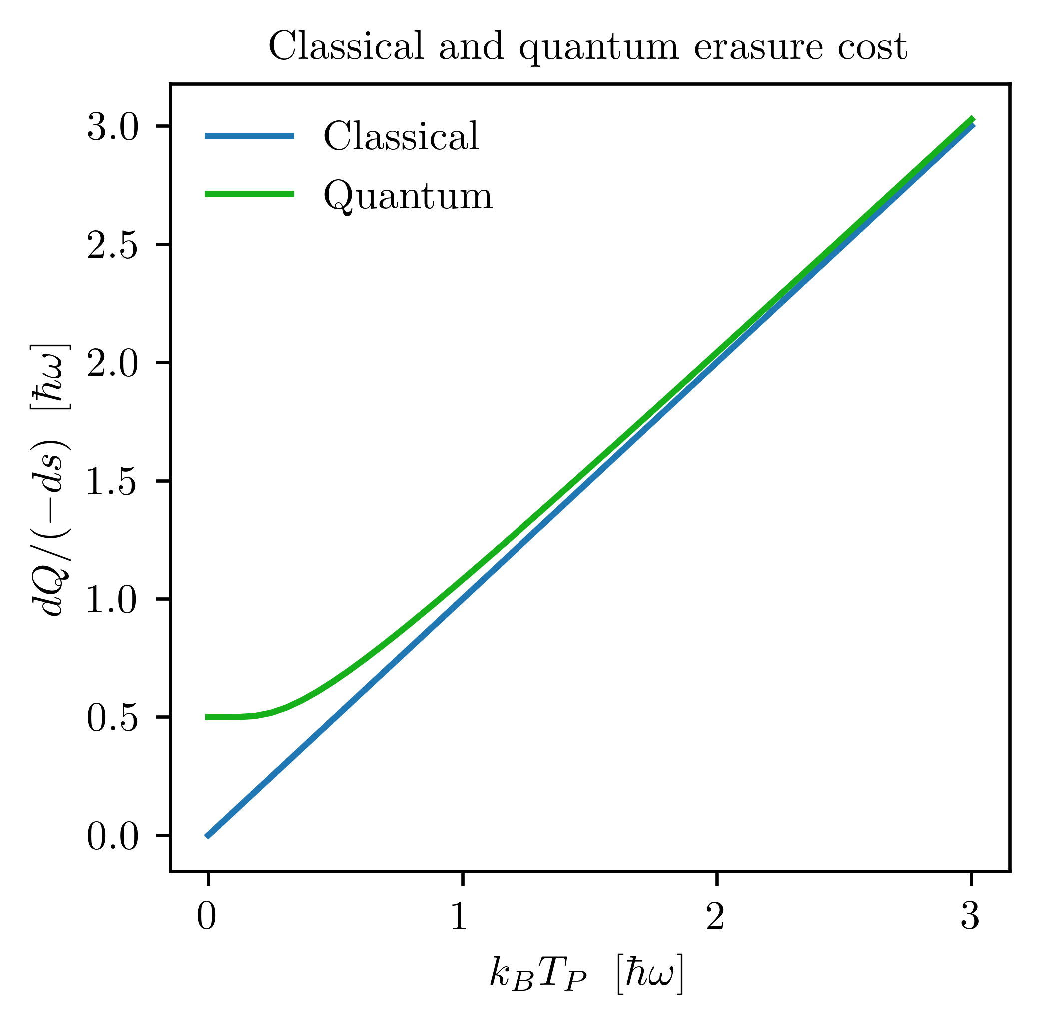
In Fig. 1 we plot the two Landauer bounds (8) and (20) as a function of temperature. Observe that they agree at high temperatures, and at low temperature (when , the quantum heat cost per bit asymptotically approaches a constant value while the classical heat cost per bit goes to zero.
III Landauer’s principle for polarizing beamsplitters
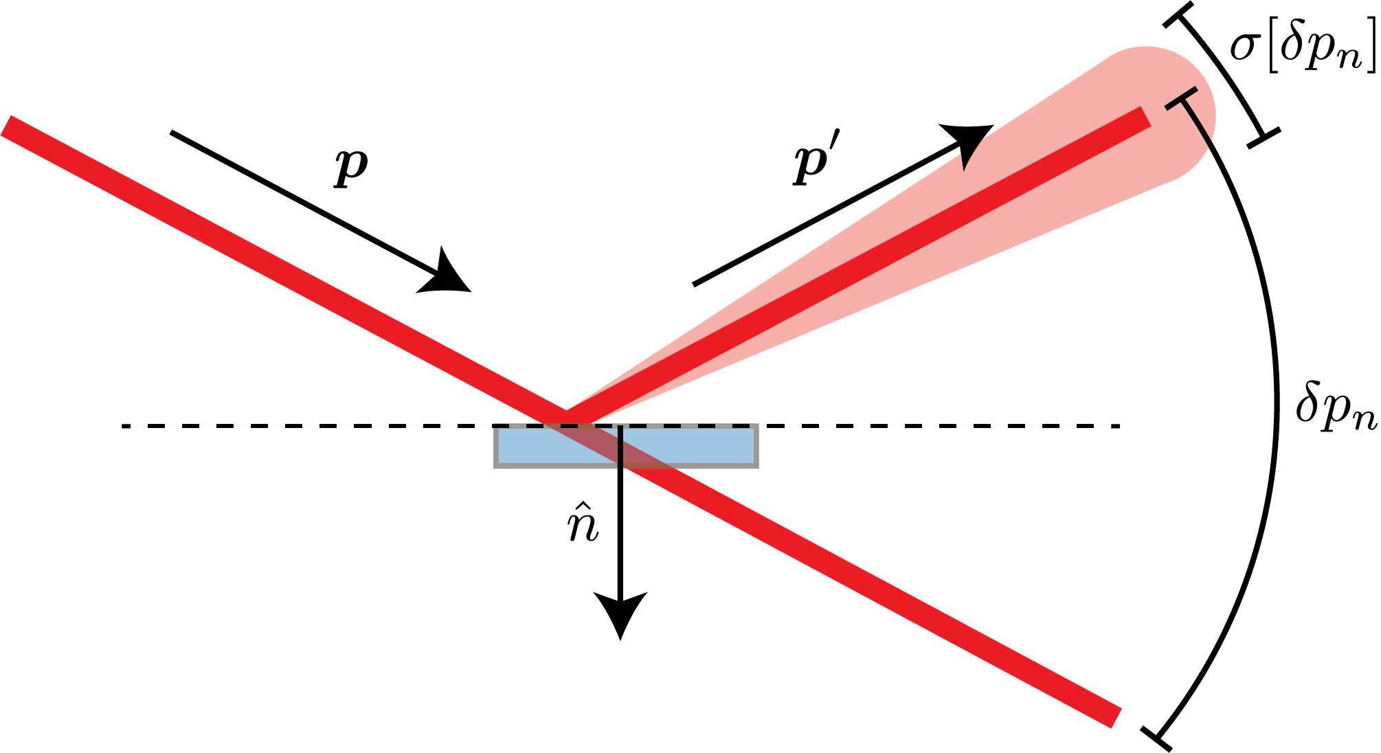
Another optical element that is subject to dissipation is a polarizing beamsplitters (PBS). Note that it is possible to produce linearly polarized light with a PBS which transmits horizontally polarized light and reflects vertically polarized light in a different direction. In this case, rather than being absorbed, the vertically polarized output is simply sent elsewhere, cf. Fig. 2. It is not clear that there is any nonzero amount of heat which must be generated in this process, which is often assumed to be non-dissipative [76]. In what follows we show that there is a minimal amount of dissipation which scales with temperature.
III.1 Semi-classical description
We first treat the PBS semi-classically, meaning we do not involve the quantum state of light, although we consider it to be made up of pointlike particles; in other words we are using the Newtonian corpuscular model [77]. Each photon is assumed to have either horizontal or vertical polarization, with each photon’s polarization an independent random variable, have probability one half of being vertically polarized and probability one half of being horizontally polarized. The PBS itself is assumed to have mass and temperature , and the photons are assigned a frequency . We show (see Appendix C), under the assumption that the reflected photons are locally unavailable, that the following lower bound on dissipation holds
| (21) |
Equation (21) relates logical information processed to dissipation cost for the semiclassical PBS.
This result is similar to Landauer’s principle in that it is a lower bound on heat generation which is proportional to the amount of logical information processed. However it differs in that it does not require any information to be “erased” per se. In our treatment we have assumed that light which is reflected by the beamsplitter is no longer accessible locally, which leads to dissipation. This is an instance of the more general phenomenon of modularity dissipation [78], whereby locally accessible information is transformed into global correlations across different parts of a system, which cannot be exploited due to physical constraints.
III.2 Quantum non-conservation cost
The result of the previous section was based on the global conservation of momentum and on the assumption of modularity, which prevents the exploitation of global correlations. This reasoning can be generalized to any information processing scheme which locally does not conserve quantities which are globally conserved, even if the desired logical operation is invertible. Here we give an example of this non-conservation cost in a quantum system which is equivalent to the PBS.
Consider the action of the polarizing beamsplitter (PBS) in the one photon subspace. The basis states of this subspace are
| (22) |
With this basis ordering the PBS unitary is then given by the following matrix
| (23) |
The PBS can therefore be thought of as a CNOT acting on a two qubit system, whose control qubit is the polarization degree of freedom and whose target degree of freedom is the path, for the one-photon subspace [79]. However, since the components of angular momentum are globally conserved, it is not possible to implement this operation deterministically unless there is access to a bath which can absorb the change in angular momentum. It has been realized that global conservation laws constrain the possible fidelity of quantum gates [80, 81], although to our knowledge this has not been applied to finding the thermodynamic cost of quantum gates under an assumption of modularity.
We assume that the two-qubit register and the bath are initially separable. The target qubit is known to be in the zero state, the control qubit is in the completely mixed state, and the bath is in an arbitrary state
| (24) |
where the bath is a register of qubits. As it is not possible to actually implement the CNOT exactly, by the previous arguments, we will assume it is implemented with some error bound . This is similar to the C-maybe interaction that has been studied in the context of quantum Darwinism [82, 83, 84]. Explicitly, we have
| (25) |
We show in Appendix D that the loss of purity on the bath is bounded below by
| (26) |
This implies that for error there is a nonzero loss of purity on the bath as a result of the CNOT operation, and the minimal loss of purity decreases exponentially with the size of the bath.
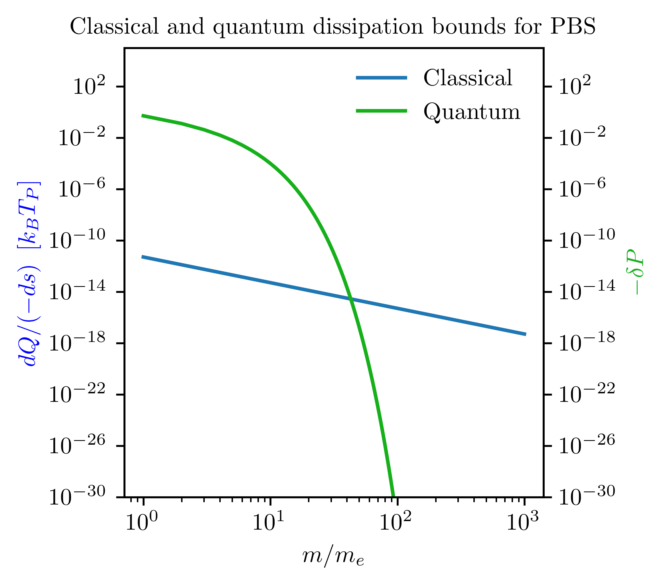
Figure 3 gives a comparison of the bounds given by Eqs. (21) and (26), plotted as a function of system size. It is assumed that in the quantum case the register is made up of electrons, so the number of spins is simply . However, the two equations give lower bounds on the change in different quantities (heat and purity), so they cannot be compared directly. We still may get an idea of how the order of magnitude of the quantum and classical bounds compare at different system sizes. The plot shows that there for the classical bound dominates and for the quantum bound becomes more relevant.
IV Quantum Master Equation for Linear Polarizers
The above analysis makes it apparent that a more rigorous treatment of optical elements as genuinely quantum devices is required. To this end, we now consider the propagation of light through an ALP, and model this as a dynamical process using a quantum master equation. The ALP is conceptualized as a series of layers through which the light propagates, interacting with each layer in turn. Each layer is modeled as a PBS, which allows for noise photons to enter from the environment as well as for losses of photons to the environment due to attenuation. To set up this model, we first give the quantum description of the PBS.
IV.1 Quantum polarizing beamsplitter
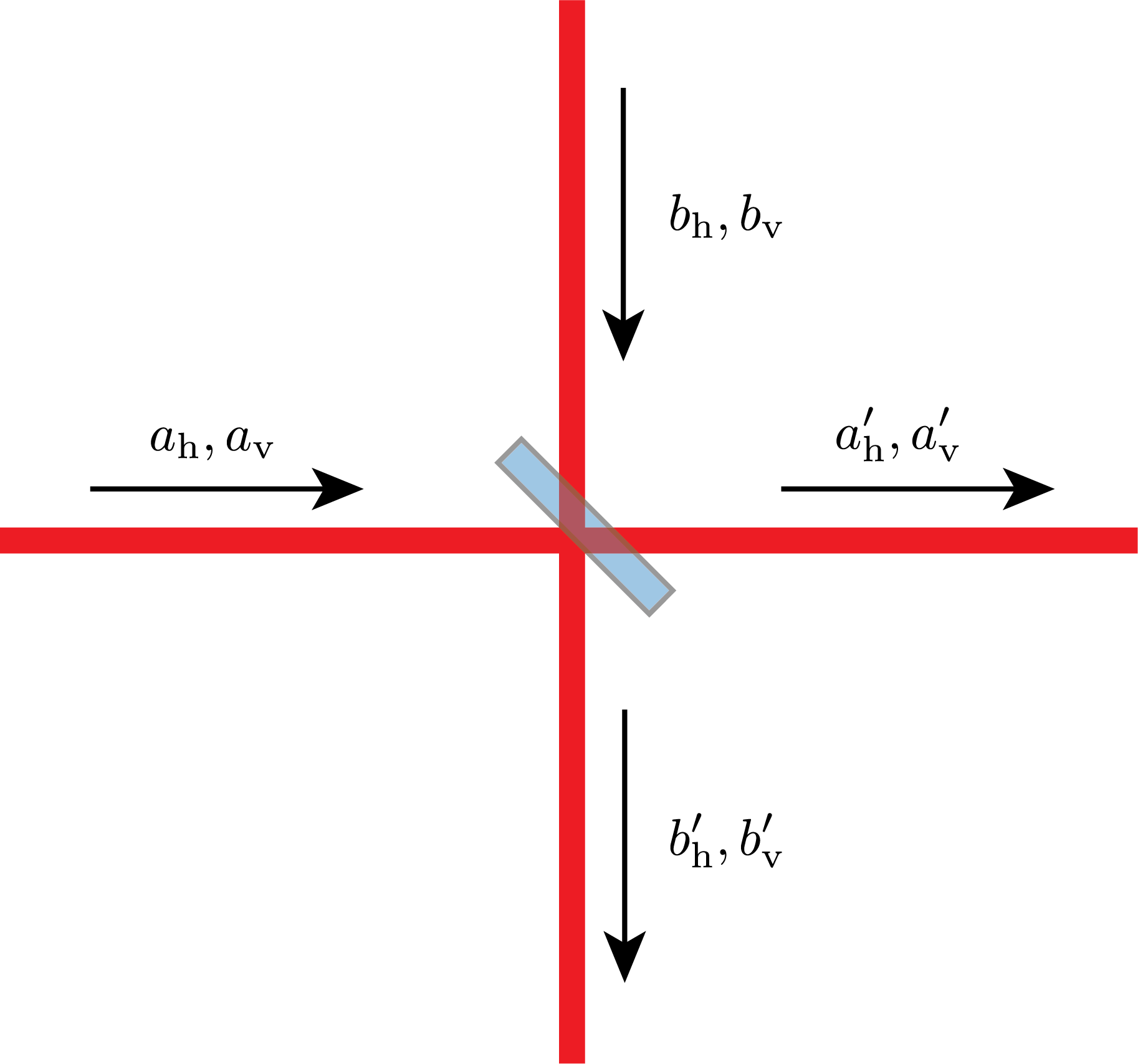
The PBS has two input ports, each with two polarization modes. We label the two polarization modes of one input port an , and similarly use and for the other input port (these will later be the annihilation operators for the input ports). The corresponding output ports are labeled , , , and (See Fig. 4).
The behavior of the PBS is easily described in the Heisenberg picture, where the operators are transformed by a scattering matrix
| (27) |
The PBS scattering matrix for the PBS may be taken to be
| (28) |
where and are the transmission and reflection coefficients, satisfying . We will therefore use the parameterization , . We can also describe PBS whose transmission and reflection axes are rotated by an angle . In this case the scattering matrix is
| (29) |
where
| (30) |
As is shown in Appendix F, the Schrödinger picture evolution operator on the Hilbert space of quantum states can be evaluated as
| (31) |
In this case we find
| (32) |
where
| (33) |
| (34) |
and
| (35) |
The density matrix is then transformed by a unitary map
| (36) |
Finally, the quantum state exiting the PBS is given formally by
| (37) |
where is the Gibbs state at the temperature of the environment.
IV.2 Multilayer model of the linear polarizer
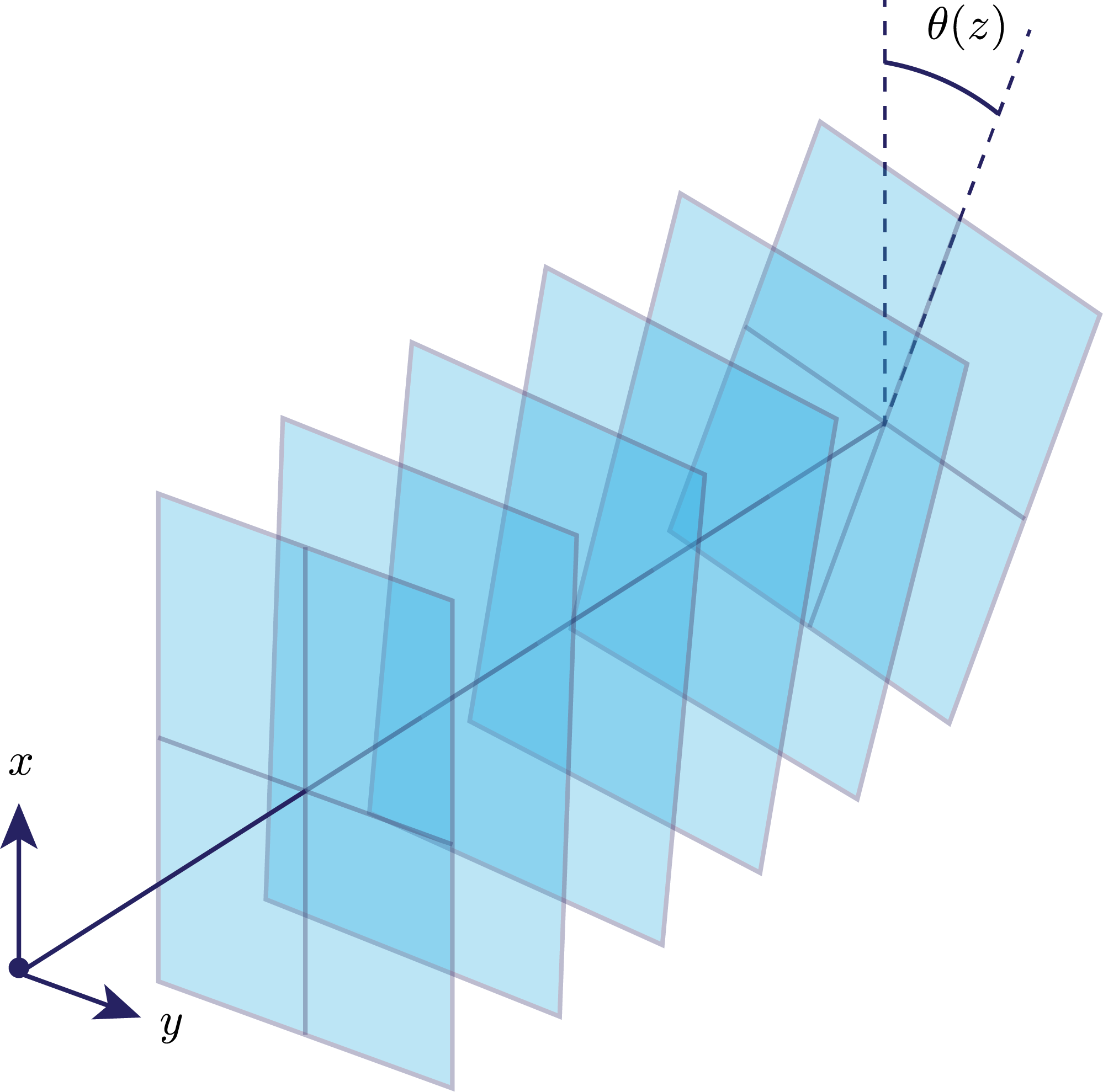

We model the linear polarizer as a sequence of PBS elements at randomized angles which are drawn from a thermal distribution. These PBS elements represent physical objects (for example, the nanoparticles in a nanoparticle-based polarizer), which are in uncertain configurations due to thermal energy. Initially the system is in some mixed state of the form of Eq. (43). At each layer the state is transformed using Eq. (37). We also allow the angle of each polarizer to be different, so the th step of the evolution is given by
| (38) |
Equation (38) is of the form of a so-called collision model or repeated interaction scheme [61, 85, 86].
We see from Eq. (32) that there is a continuum limit as long as is taken to zero as goes to zero. We set . Then to first order in , we have
| (39) |
This leads to the following master equation
| (40) |
where
| (41) |
It has been shown by Lorenzo et al. [11] that for collision models of this form, the following form of Landauer’s principle is observed
| (42) |
which is again the desired result.
IV.3 Single-photon states at low temperature
To make contact with experimentally realistic scenarios we are concerned with photons of optical frequency ( Hz), so at room temperature ( meV) the probability of finding photons in a given mode is proportional to . We therefore assume that the number of photons in the vacuum ports is always initially. We are effectively treating the environment as being at zero temperature for the purposes of thermal radiation. However, we will not assume zero temperature for the mechanical degrees of freedom of the polarizer itself which contribute to uncertainty in the transmission axis.
Suppose that incident on the input port of a PBS there is a general mixed state belonging to the subspace with at most one photon,
| (43) |
The state of the two input ports and combined is then
| (44) |
We are concerned with the reduced density matrix for the input mode, . The evolution of is given by
| (45) |
The evolution given by Eq. (37) is a CPTP map [87], and therefore can be given in terms of Krauss operators. For this particular case, it can be expressed in terms of two Krauss operators which depend on , and
| (46) |
Explicitly, the Krauss operators are,
| (47) |
and,
| (48) |
Equations (46), (47), and (48) completely specify the evolution of the density matrix as the single photon propagates through a single layer of the polarizer at low temperature. To simulate the evolution in the multilayer model, the angle for each polarizer is drawn from a thermal distribution
| (49) |
where is a physical parameter of the polarizing material which characterizes the energy required to change the orientation of polarizing elements from their (mechanical) equilibrium positions. The resulting maps are applied one after another. For we get a particularly simple evolution
| (50) |
In Appendix E, we consider the Heisenberg picture description of a single application of the map with a random angle drawn from the distribution (49). It is found that an adjoint map can be defined which gives evolved operators satisfying a modified commutation relation
| (51) |
where .
In Eq. (51) we observe the direct impact of the noise in the PBS on the optical signal. The quantum mechanical communtation relations “degrade” as a function of temperature, which is nothing but another way of looking at effects of decoherence.
IV.4 Numerical study of the low-temperature limit
Using the above formalism we simulate the evolution of the quantum state of light, limited to the photon subspace, and assuming low temperature, that is . This simulation allows us to discuss some qualitative aspects of the polarization process. We initialize the system in the state
| (52) |
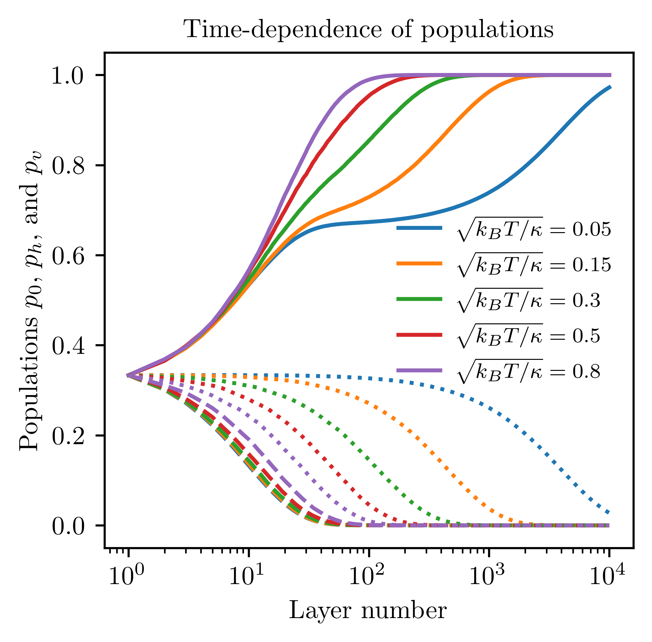
Then the CPTP map is iterated for layers with . A range of temperatures are chosen in the interval . We find that the population decays very quickly, as expected, falling to near zero after less than one hundred layers. The horizontal population takes a longer time to decay. As temperature increases, decays more slowly and decays more quickly, until the two polarizations behave near identically for . At low temperature, due to the lag between absorption of vertically and horizontally polarized light, the vacuum population has a plateau at intermediate times (see Fig. 7).
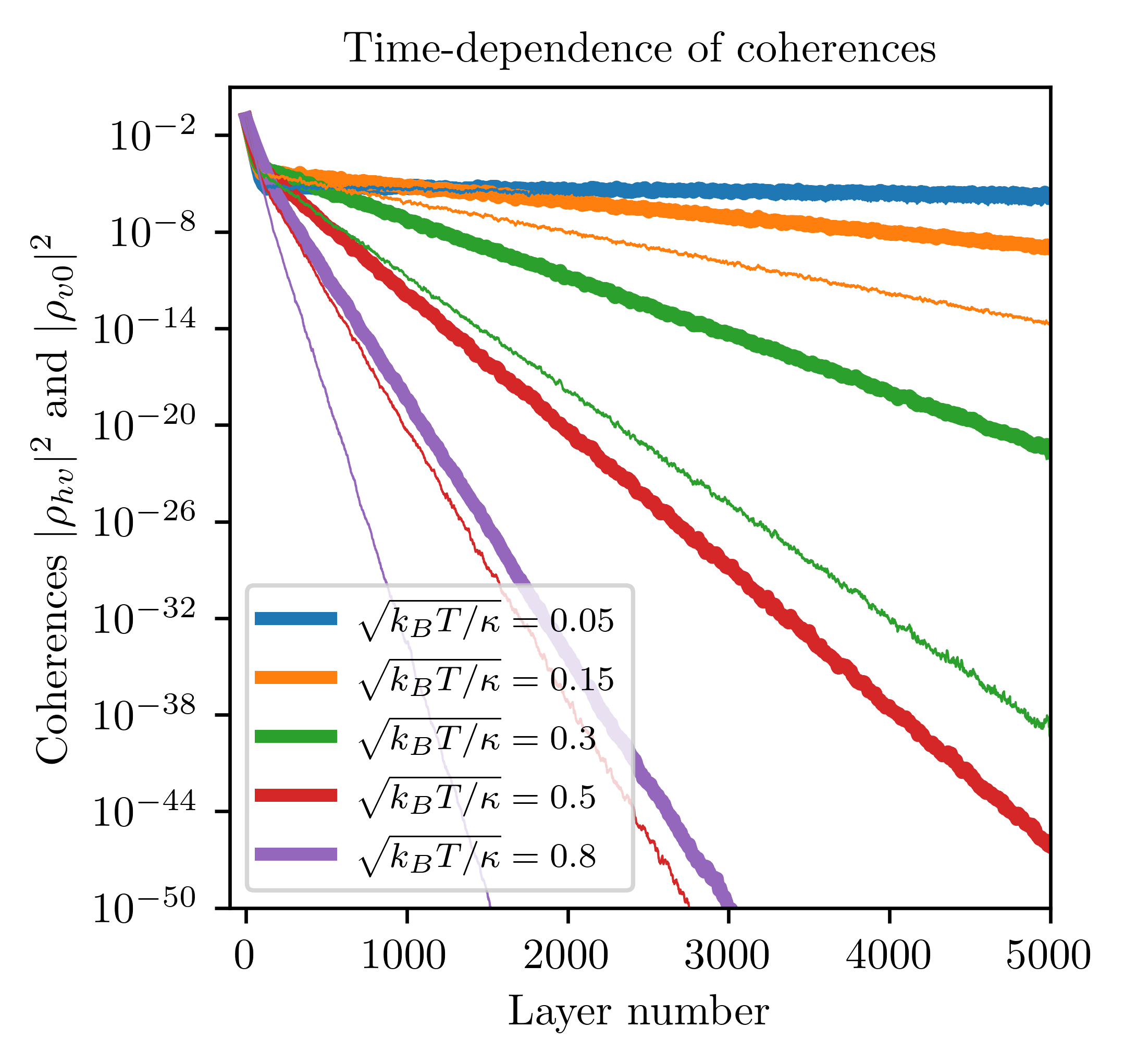
We see from Fig. 8 that the coherences and decay exponentially, with the horizontal-vacuum coherence decaying faster. The decay of coherence occurs faster at higher temperatures. This result is in line with our expectations, given that decoherence has been found to be enhanced at higher temperatures in a variety of physical systems [88, 89, 90].
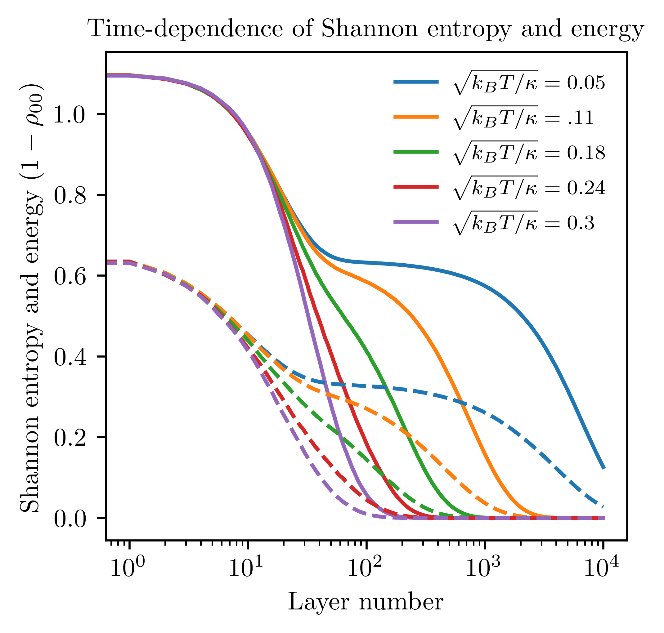
The Shannon entropy is evaluated at all times, and it is found to decrease monotonically. The energy is proportional to , and also decreases monotonically. Figure 9 shows the time dependence of the energy and Shannon entropy, with both display the plateau feature at low temperatures discussed earlier.
Landauer’s principle concerns the change in heat relative to the change in Shannon entropy, which can be expressed as the derivative along a system trajectory. Since we assume , we are therefore interested in the derivative along some system trajectory. Although this ratio is related to temperature, it is not given by any function of temperature given that the system is out of equilibrium. We plot the energy against the Shannon entropy for 100 realizations of the random process at various temperatures. For each realization, the angles of the polarizer layers have been drawn from a Boltzmann distribution at the given temperature, and the initial conditions are always those given by Eq. (52).
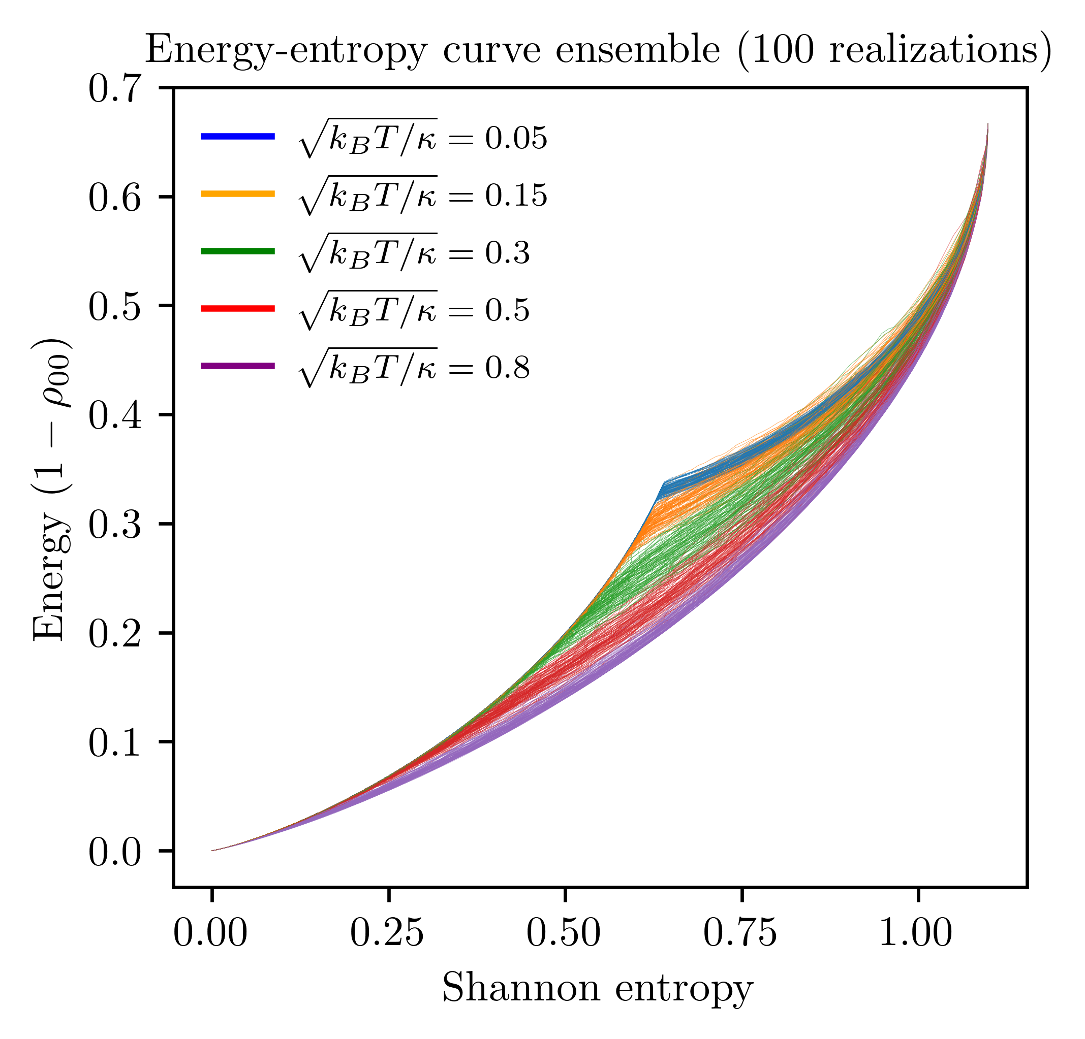
Figure 10 shows that the energy always increases monotonically with Shannon entropy, as expected. Interestingly, as temperature approaches zero, a discontinuity of the slope appears near . This can be explained by the plateaus appearing in Fig. 9 at low temperature. On the plateaus, both the entropy and energy are nearly constant, although many layers of the polarizer are traversed. After the plateau, the relative slope of the energy and entropy is different than what it was before, and so a discontinuity of the slope appears when the energy and Shannon entropy are plotted against each other.
V Temperature-dependent quantum eraser
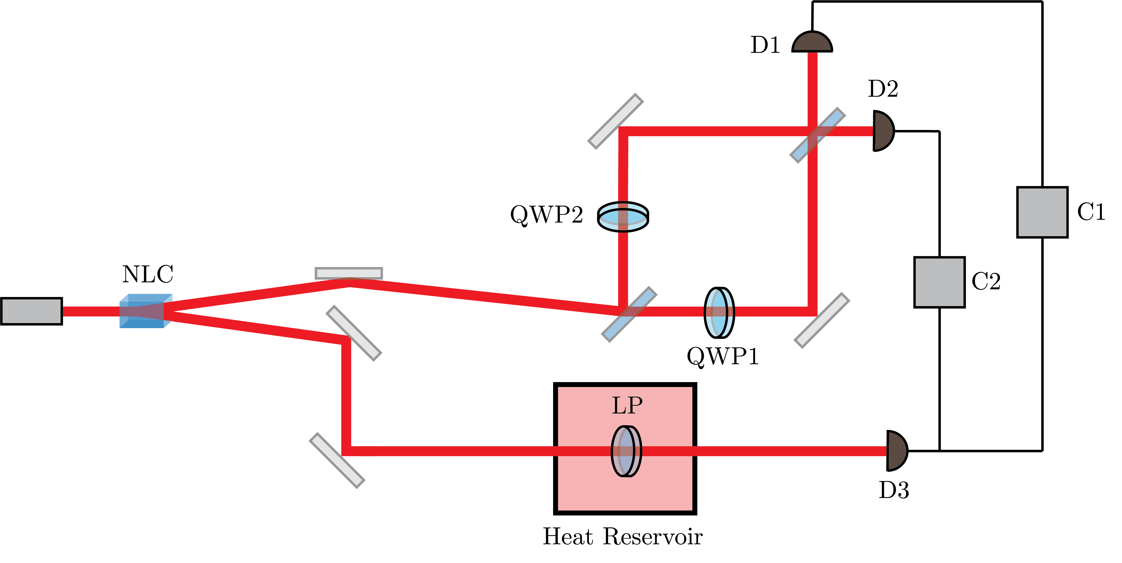
We conclude the analysis with an experimentally testable consequence of our findings. We have developed a theoretical model for the effect of temperature on the evolution of a single-photon state through a polarizing medium, and our model predicts that at higher temperature there is enhanced decoherence. We now propose an experimental test of this, which is a modified quantum eraser experiment where the linear polarizer used to measure one of the photon’s polarization is in contact with a heat reservoir at temperature . In the quantum eraser experiment [64, 67, 91, 66, 92, 65] there are two photons, called the signal and idler photons. The signal photon may be either horizontally or vertically polarized, or it may be absorbed by the polarizer so it lives in a three-dimensional Hilbert space spanned by the vectors . The idler photon may be either horizontally or vertically polarized, and it may go down path or path of the interferometer, so it lives in a four-dimensional Hilbert space spanned by the vectors . So the state of the two photons together belongs to a -dimensional Hilbert space spanned by the following states
| (53) | ||||
These states can be expressed as , where , , and . Then in general we have a density matrix of the form
| (54) |
The full density matrix can be written as a array of submatrices, where the indices in the array correspond to the idler photon and the indices of each submatrix correspond to the signal photon.
| (55) |
To evolve the density matrix forward by one step, we use Eq. (37). This gives
| (56) |
The initial condition for the quantum eraser experiment is a Bell state in the polarization basis for the two photons:
| (57) |
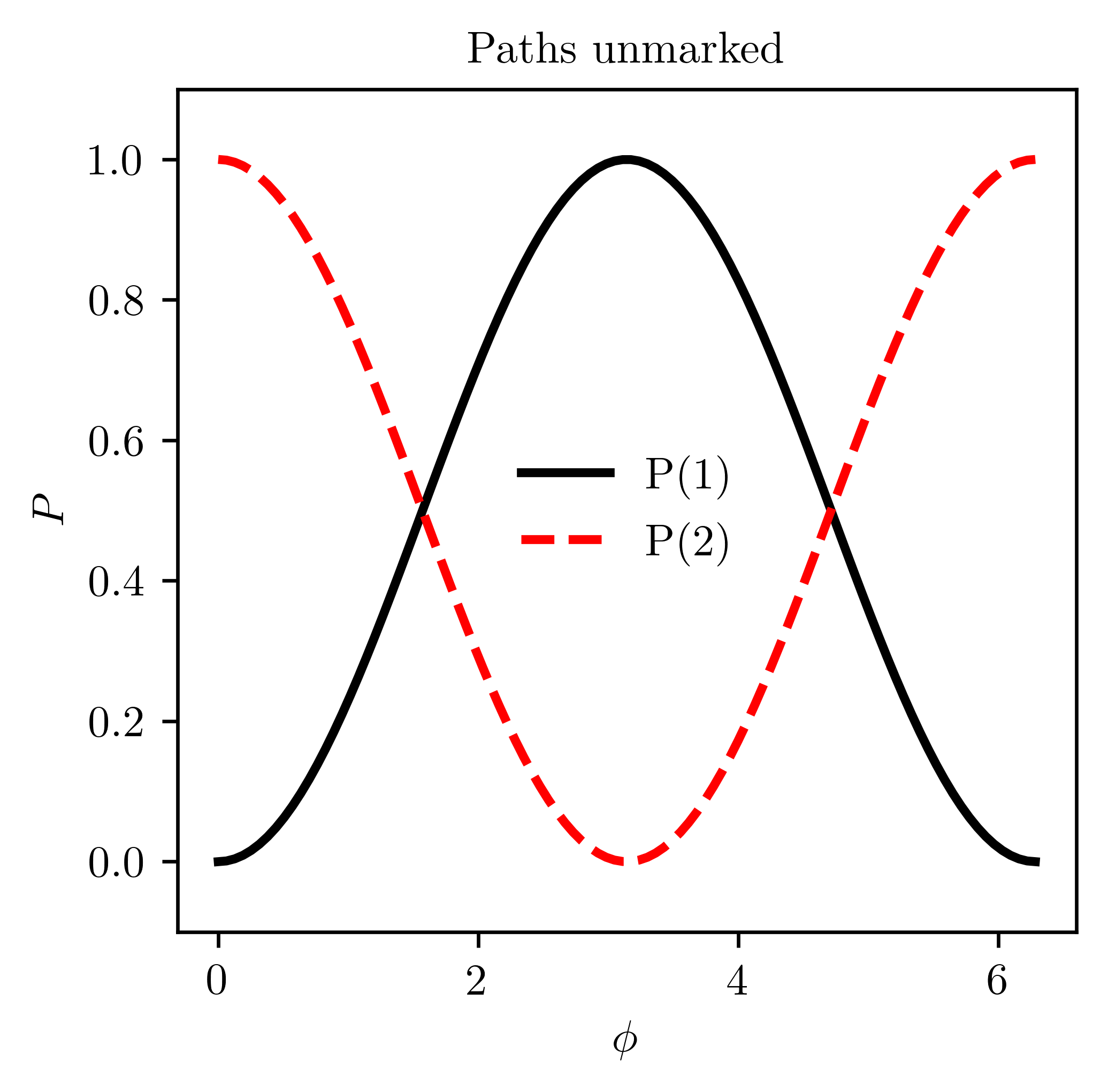
First, a beamsplitter is applied to the idler photon. There are two distinct configurations for the interferometer, one in which the paths are “marked” and the other the paths “unmarked”. For the marked configuration there is a quarter wave plate (QWP) in each path of the interferometer (see Fig. 11). One of the QWPs is at an angle of radians, the other at an angle of radians. For the unmarked configuration there are no QWPs. First we simulate what happens in the unmarked configuration when there is no measurement made on the signal photon, and recover the standard result of a simple Mach-Zehnder interferometer experiment (see Fig. 12) [93].
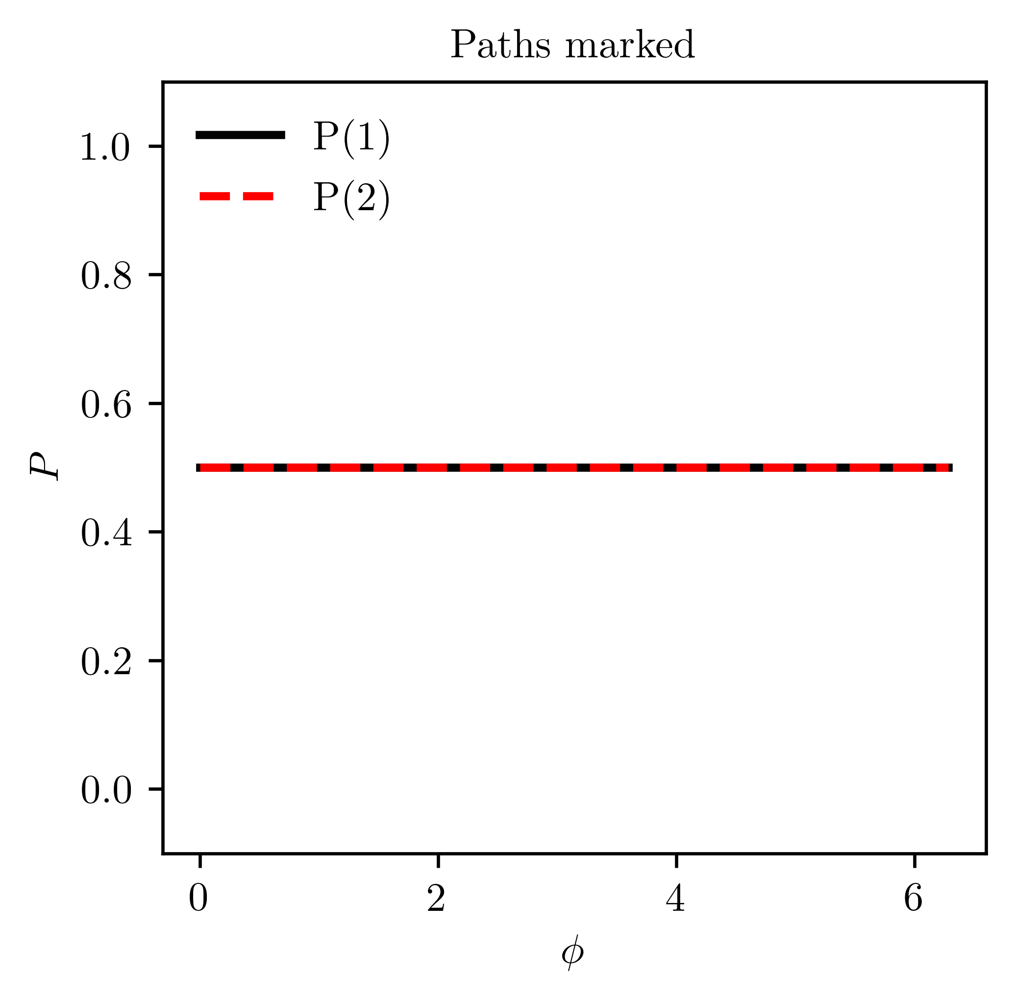
Next we look at the marked configuration, again with no measurement made on the signal photon, the result of which is shown in Fig. 13. We see that the interference pattern is now lost.
We then make a measurement on the signal photon with a linear polarizer at an angle from the vertical, resulting in a restoration of the interference pattern.
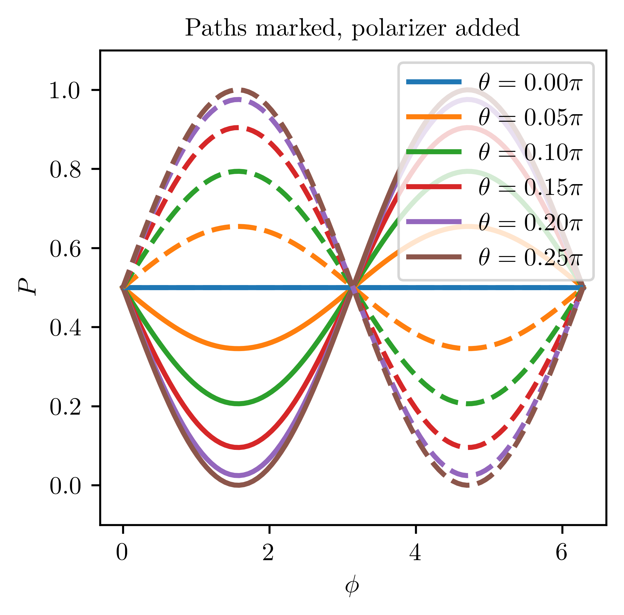
We see that the interference pattern is gone when , and is completely restored for , which is the main result of the traditional quantum eraser experiment (see Fig. 14). The variation in the interference pattern is most pronounced at a path phase difference of .
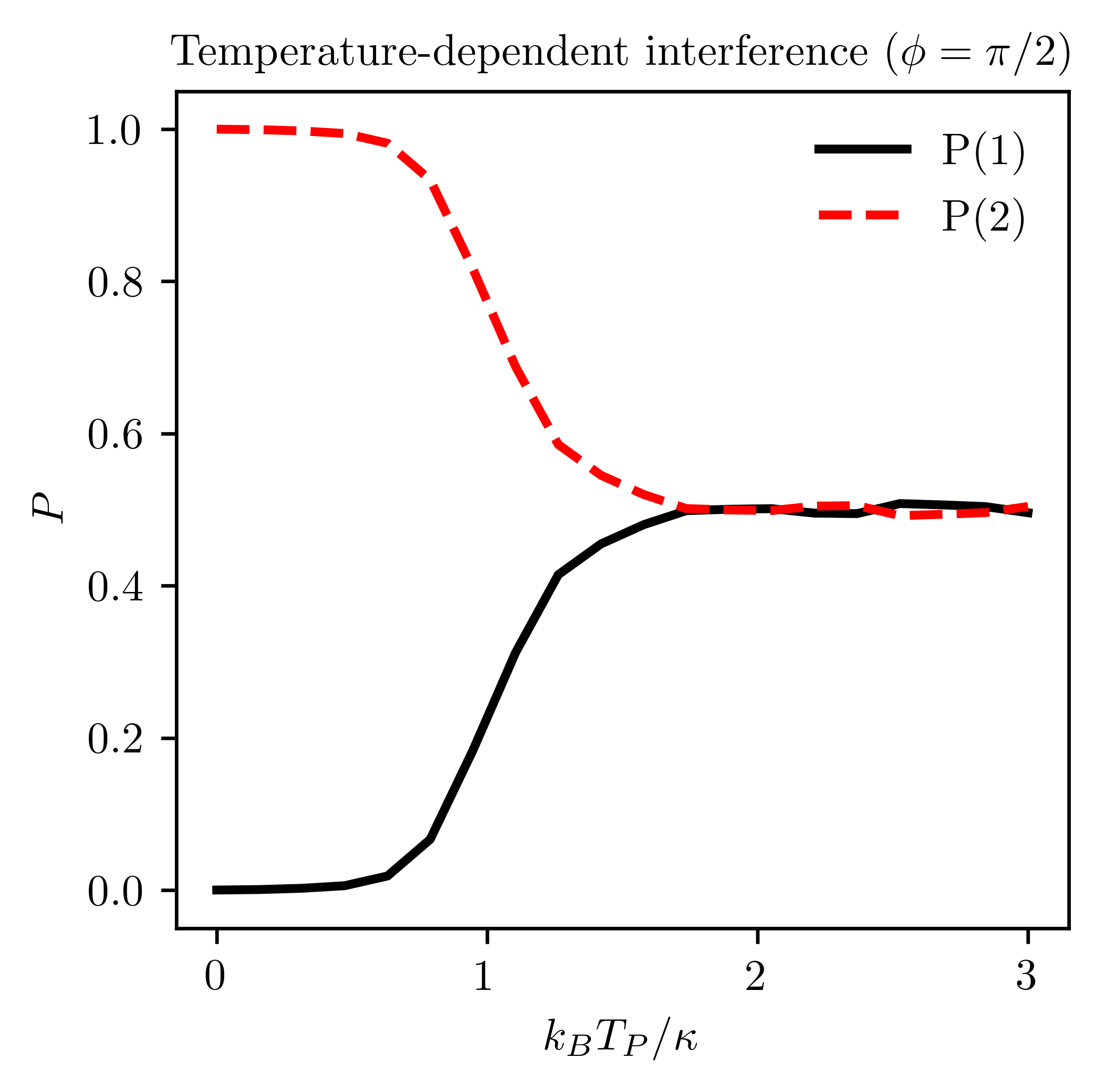
We see from Fig. 15 that the effect of quantum erasing is temperature dependent. In particular, as temperature is increased, the ability of the polarizer to restore interference is suppressed, and eventually goes away entirely.
VI Concluding remarks
Our analysis has provided insight into the (quantum) thermodynamics of linear polarizers; we have given explicit forms of Landauer’s principle for both absorbing linear polarizers and polarizing beamsplitters. We have also developed a formalism that incorporates the thermal energy contained in mechanical degrees of freedom of a polarizer, and used this model to investigate the time-dependent dynamics of the polarization process. We have provided a qualitative description of the dependence of this process on temperature, and proposed an experiment to test the temperature-dependence of decoherence via a quantum eraser apparatus.
Some questions have been left unanswered which warrant further analysis. A full solution of the master equation derived for the quantum absorbing polarizer, even in the low temperature limit and the single photon subspace is lacking. We also have not yet written a master equation valid when is on the order of at least . Answering these and other questions will provide guidance for optimal control of optical polarization states. This is expected to be particularly challenging task when is nearly of the order of , since then environmental noise becomes significant. Therefore we hope to extend our results with special attention paid to deriving a master equation valid in the high temperature limit. It is then desirable to find bounds on the minimum dissipation required to perform various tasks in such an environment, including the version of Landauer’s principle in Eq. (42).
Acknowledgements.
We would like to thank Todd Pittman, Alejandro Rodriguez Perez, Steve Campbell, and Pat Eblen for enlighting discussions. M.A. gratefully acknowledges support from Harry Shaw of NASA Goddard Space Flight Center. N.M.M. acknowledges support from AFOSR (FA2386-21-1-4081, FA9550-19-1-0272, FA9550-23-1-0034) and ARO (W911NF2210247, W911NF2010013). S.D. acknowledges support from the John Templeton Foundation under Grant No. 62422.Appendix A Derivation of classical Landauer’s principle
Recall that for a random vector of dimension , and with covariance matrix , the entropy is upper bounded by that of the normal distribution [94, 95]
| (58) |
We regard as a bivariate distribution over both the real and imaginary parts of . Note that in general , so
| (59) |
We assume that after the light has passed through the polarizer, it is in a thermal distribution with temperature , which is associated with the polarizer itself. Therefore the energy is and the entropy is
| (60) |
Consequently, the decrease in Shannon entropy is at most
| (61) |
Since there is no work reservoir, all lost energy is dissipated as heat, and we have
| (62) |
Using and the upper bound on then gives
| (63) |
Appendix B Derivation of quantum Landauer’s principle
Again using Eq. (58), we find that
| (64) |
Due to Eq. (12) this is bounded above by
| (65) |
We again assume that the light is in a thermal state after leaving the polarizer. The thermal state has Wigner function [96, 97]
| (66) |
where is given by
| (67) |
or alternatively
| (68) |
Since the thermal Wigner function (66) is positive, the final Wigner entropy is defined, and is given by
| (69) |
We can write
| (70) |
We once again equate the heat to the lost energy
| (71) |
and hence
| (72) |
Appendix C Minimal dissipation for the semi-classical PBS
Let be the unit vector which is perpendicular to the PBS surface and is pointing into the bulk. The PBS and the photon have momenta and respectively in the lab frame. We define and as the inward normal components of and . Using a Lorentz transformation, this component of the photon’s momentum in the rest frame of the PBS is then [98]
| (73) |
where is the Lorentz factor and is the frequency in the lab frame. Because the PBS momentum is nonrelativistic we set . We assume that in the rest frame of the PBS, the photon’s angle of reflection is the same as the angle of incidence, although this is only approximately true due to the transfer of energy from the photon to the PBS. That is, we set
| (74) |
Thus in the lab frame, the photon’s momentum after the collision differs from its initial momentum by an amount
| (75) |
To ensure that a reflected photon can be distinguished from a transmitted photon, the difference in momentum of the two paths should be greater than the uncertainty in momentum of the reflected photon, that is
| (76) |
This condition is in effect a restriction on the statistical distance (as defined by Wootters [99]) between the momenta of the transmitted and reflected photons. And so from Eq. (75), and the fact that we have
| (77) |
Because the PBS is at finite temperature , we assume its momentum is initially given by the canonical distribution
| (78) |
and therefore
| (79) |
Next note that for momentum to be conserved, the momentum of the PBS must also change by an amount . In our convention is positive by definition, so
| (80) |
Many photons are incident on the device, one after another. For each photon, the initial momentum is the same, and so is very nearly the same for each reflected photon, so we treat it as constant. We assume that each photon is vertically polarized with probability one half and horizontally polarized with probability one half. So with probability one half is increased by as each photon passes. Therefore after photons have come, the total change in the momentum of the PBS is given by a binomial distribution
| (81) |
By the de Moivre-Laplace theorem [100], for large the distribution approaches a Gaussian with variance . Therefore,
| (82) |
Recall that the sum of two Gaussian random variables is Gaussian, with variance equal to the sum of the two original distributions’ variances. Using the variance of then gives
| (83) |
Then, using the formula for the Shannon entropy of a Gaussian, we have
| (84) |
| (85) |
Our approximation is only valid for , and in this limit we have
| (86) |
After many photons have passed, is in an equilibrium distribution, so we can equate the Shannon entropy with the thermal entropy. Then the heat dissipated as a single photon passes is
| (87) |
The information carried by the photon is one bit, as per our assumption, so we may write this as
| (88) |
Appendix D Minimal loss of purity for quantum PBS
The joint state of the system and the bath is acted on by a unitary operator . Define the quantum state
| (89) |
and
| (90) |
where . Therefore, we write
| (91) |
Now suppose that the bath is composed of qubits. For conservation of angular momentum to hold, we require that
| (92) |
where is the Pauli Z-matrix. The noisy CNOT is implemented on the system qubits within accuracy , meaning
| (93) |
Employing the Cauchy-Schwarz inequality we obtain
| (94) |
and hence
| (95) |
and
| (96) |
Finally, we can then write
| (97) |
which further leads to
| (98) |
Thus, the purity of the final state is
| (99) |
Note that the last term can also be expressed as
| (100) |
Now, since the purity of the states and cannot exceed the purity of , we have
| (101) |
Using the Cauchy-Schwarz inequality again we obtain
| (102) |
and with for we can have
| (103) |
Collecting expressions we can further write
| (104) |
and finally
| (105) |
which we rewrite (as in the main text) as
| (106) |
Appendix E Derivation of modified commutation relation
Consider the case where a PBS is at an unknown angle , with some probability density . If the state of the two input modes is given some density matrix , then the output density matrix is
| (107) |
where we define as the quantum channel which propagates the density matrix in the Schrödinger picture. There is an adjoint map which can be used to propagate operators in the Heisenberg picture, and satisfies [101]
| (108) |
for all density matrices and operators . In fact it is easily seen that is given by
| (109) |
Then using Eq. (27) we see that the adjoint map acting on the annihilation operators can be expressed as
| (110) |
where we have defined the ensemble-averaged scattering matrix as
| (111) |
Note that the evolved operators do not necessarily obey the standard Dirac commutation relation anymore since need not be unitary. While we can evaluate expectation values using Eq. (108), we cannot build new operators or states using the evolved operators. However, many useful operators are expressed in terms of products of annihilation operators. We will consider the class of operators which can be written as
| (112) |
To see how such an operator evolves under these dynamics, we first note
| (113) |
where we defined
| (114) |
Therefore by Eq. (109) we have
| (115) |
where
| (116) |
We will now assume that is Gaussian, with some temperature
| (117) |
Then evaluating Eq. (111), we find that
| (118) |
where . We can then express the primed annihilation operators as
| (119) |
and
| (120) |
Note that is a monotonically increasing function of temperature and at , and hence Eqs. (119) and (120) clearly show the influence on increasing temperature on the propagation of the annihilation operators. For zero temperature we have
| (121) |
meaning the model behaves as a PBS at definite angle, as expected. In the limit of infinite temperature , and we find that
| (122) |
and
| (123) |
meaning that horizontally polarized and vertically polarized light are not distinguished by the device. The primed annihilation operators do not obey the standard commutation relations. Instead we find that
| (124) |
Appendix F Construction of the Evolution Operator
In this last appendix, we show that the two treatments we gave in the Heisenberg and Schrödinger picture are in fact equivalent. This formulation is not a new result but we have included it for convenience (for similar calculations see e.g. [102, 103]). Recall that the evolution operator was obtained as follows, for
| (125) |
where is the Unitary scattering matrix. Then
| (126) |
and
| (127) |
Since is unitary, is anti-Hermitian. Using this fact and interchanging and in the first summation, we get
| (128) |
and
| (129) |
Thus, we have
| (130) |
The unique solution to this equation is
| (131) |
References
- Raymer and Monroe [2019] M. G. Raymer and C. Monroe, The US national quantum initiative, Quantum Sci. Technol. 4, 020504 (2019).
- Deffner and Campbell [2019] S. Deffner and S. Campbell, Quantum Thermodynamics (Morgan & Claypool Publishers, 2019).
- Parrondo et al. [2015] J. M. R. Parrondo, J. M. Horowitz, and T. Sagawa, Thermodynamics of information, Nature Physics 11, 131 (2015).
- Landauer [1961] R. Landauer, Irreversibility and Heat Generation in the Computing Process, IBM J. Res. & Dev. 5, 183 (1961).
- Piechocinska [2000] B. Piechocinska, Information erasure, Phys. Rev. A 61, 062314 (2000).
- Deffner and Jarzynski [2013] S. Deffner and C. Jarzynski, Information Processing and the Second Law of Thermodynamics: An Inclusive, Hamiltonian Approach, Phys. Rev. X 3, 041003 (2013).
- Boyd and Crutchfield [2016] A. B. Boyd and J. P. Crutchfield, Maxwell demon dynamics: Deterministic chaos, the Szilard map, and the intelligence of thermodynamic systems, Phys. Rev. Lett. 116, 190601 (2016).
- Boyd et al. [2016] A. B. Boyd, D. Mandal, and J. P. Crutchfield, Identifying functional thermodynamics in autonomous Maxwellian ratchets, New J. Phys. 18, 023049 (2016).
- Boyd et al. [2018a] A. B. Boyd, D. Mandal, and J. P. Crutchfield, Thermodynamics of modularity: Structural costs beyond the Landauer bound, Phys. Rev. X 8, 031036 (2018a).
- Hilt et al. [2011] S. Hilt, S. Shabbir, J. Anders, and E. Lutz, Landauer’s principle in the quantum regime, Phys. Rev. E 83, 030102 (2011).
- Lorenzo et al. [2015a] S. Lorenzo, R. McCloskey, F. Ciccarello, M. Paternostro, and G. Palma, Landauer’s Principle in Multipartite Open Quantum System Dynamics, Phys. Rev. Lett. 115, 120403 (2015a).
- Van Vu and Saito [2022] T. Van Vu and K. Saito, Finite-Time Quantum Landauer Principle and Quantum Coherence, Phys. Rev. Lett. 128, 010602 (2022).
- Goold et al. [2015] J. Goold, M. Paternostro, and K. Modi, Nonequilibrium Quantum Landauer Principle, Phys. Rev. Lett. 114, 060602 (2015).
- Bérut et al. [2012] A. Bérut, A. Arakelyan, A. Petrosyan, S. Ciliberto, R. Dillenschneider, and E. Lutz, Experimental verification of Landauer’s principle linking information and thermodynamics, Nature 483, 187 (2012).
- Maroney [2009] O. J. E. Maroney, Generalizing Landauer’s principle, Phys. Rev. E 79, 031105 (2009).
- Norton [2011] J. D. Norton, Waiting for Landauer, Stud. Hist. Philos. Sci. Part B: Stud. Hist. Philos. Mod. Phys. 42, 184 (2011).
- Maroney [2005] O. Maroney, The (absence of a) relationship between thermodynamic and logical reversibility, Stud. Hist. Philos. Sci. Part B: Stud. Hist. Philos. Mod. Phys. 36, 355 (2005).
- Bylicka et al. [2016] B. Bylicka, M. Tukiainen, D. Chruściński, J. Piilo, and S. Maniscalco, Thermodynamic power of non-Markovianity, Sci. Rep. 6, 27989 (2016).
- Pezzutto et al. [2016] M. Pezzutto, M. Paternostro, and Y. Omar, Implications of non-Markovian quantum dynamics for the Landauer bound, New J. Phys. 18, 123018 (2016).
- Zhang et al. [2021] Q. Zhang, Z.-X. Man, and Y.-J. Xia, Non-Markovianity and the Landauer principle in composite thermal environments, Phys. Rev. A 103, 032201 (2021).
- Hu et al. [2022] H.-R. Hu, L. Li, J. Zou, and W.-M. Liu, Relation between non-Markovianity and Landauer’s principle, Phys. Rev. A 105, 062429 (2022).
- Man et al. [2019] Z.-X. Man, Y.-J. Xia, and R. Lo Franco, Validity of the Landauer principle and quantum memory effects via collisional models, Phys. Rev. A 99, 042106 (2019).
- Bremermann [1967] H. J. Bremermann, Quantum noise and information, in Proceedings of the Fifth Berkeley Symposium on Mathematical Statistics and Probability, Volume 4: Biology and Problems of Health (University of California Press, Berkeley, Calif., 1967) pp. 15–20.
- Heisenberg [1927] W. Heisenberg, Über den anschaulichen Inhalt der quantentheoretischen Kinematik und Mechanik, Z. für Phys. 43, 172 (1927).
- Bekenstein [1981a] J. D. Bekenstein, Energy Cost of Information Transfer, Phys. Rev. Lett. 46, 623 (1981a).
- Bekenstein [1973] J. D. Bekenstein, Black holes and entropy, Phys. Rev. D 7, 2333 (1973).
- Bekenstein [1974] J. D. Bekenstein, Generalized second law of thermodynamics in black-hole physics, Phys. Rev. D 9, 3292 (1974).
- Hawking [1975] S. W. Hawking, Particle creation by black holes, Comm. Math. Phys. 43, 199 (1975).
- Bekenstein [1981b] J. D. Bekenstein, Universal upper bound on the entropy-to-energy ratio for bounded systems, Phys. Rev. D 23, 287 (1981b).
- Bekenstein and Schiffer [1990] J. D. Bekenstein and M. Schiffer, Quantum limitations on the storage and transmission of information, Int. J. Mod. Phys. C 1, 355 (1990).
- Pendry [1983] J. B. Pendry, Quantum limits to the flow of information and entropy, J. Phys. A: Math. Gen. 16, 2161 (1983).
- Landauer [1987] R. Landauer, Energy requirements in communication, Appl. Phys. Lett. 51, 2056 (1987).
- Bekenstein [1988] J. D. Bekenstein, Communication and energy, Phys. Rev. A 37, 3437 (1988).
- Caves and Drummond [1994] C. M. Caves and P. D. Drummond, Quantum limits on bosonic communication rates, Rev. Mod. Phys. 66, 481 (1994).
- Blencowe and Vitelli [2000] M. P. Blencowe and V. Vitelli, Universal quantum limits on single-channel information, entropy, and heat flow, Phys. Rev. A 62, 052104 (2000).
- Lloyd et al. [2004] S. Lloyd, V. Giovannetti, and L. Maccone, Physical limits to communication, Phys. Rev. Lett. 93, 100501 (2004).
- Garbaczewski [2007] P. Garbaczewski, Information dynamics in quantum theory, Appl. Math. & Information Sciences 1, 1 (2007).
- Pei-Rong and Di [2010] G. Pei-Rong and L. Di, Upper bound for the time derivative of entropy for a stochastic dynamical system with double singularities driven by non-Gaussian noise, Chin. Phys. B 19, 030520 (2010).
- Deffner and Lutz [2010] S. Deffner and E. Lutz, Generalized Clausius inequality for nonequilibrium quantum processes, Phys. Rev. Lett. 105, 170402 (2010).
- Guo et al. [2011] Y. Guo, W. Xu, H. Liu, D. Li, and L. Wang, Upper bound of time derivative of entropy for a dynamical system driven by quasimonochromatic noise, Comm. Nonlin. Sci. Num. Sim. 16, 522 (2011).
- Guo and Tan [2012] Y.-F. Guo and J.-G. Tan, Time evolution of information entropy for a stochastic system with double singularities driven by quasimonochromatic noise, Chin. Phys. B 21, 120501 (2012).
- Bousso [2017] R. Bousso, Universal limit on communication, Phys. Rev. Lett. 119, 140501 (2017).
- Lewis-Swan et al. [2019] R. J. Lewis-Swan, A. Safavi-Naini, A. M. Kaufman, and A. M. Rey, Dynamics of quantum information, Nat. Rev. Phys. 1, 627 (2019).
- Deffner [2020] S. Deffner, Quantum speed limits and the maximal rate of information production, Phys. Rev. Research 2, 013161 (2020).
- Gisin and Thew [2007] N. Gisin and R. Thew, Quantum communication, Nat. Phot. 1, 165 (2007).
- Chen [2021] J. Chen, Review on quantum communication and quantum computation, J. Physics: Conf. Ser. 1865, 022008 (2021).
- Wehner et al. [2018] S. Wehner, D. Elkouss, and R. Hanson, Quantum internet: A vision for the road ahead, Science 362, eaam9288 (2018).
- Gisin et al. [2002] N. Gisin, G. Ribordy, W. Tittel, and H. Zbinden, Quantum cryptography, Rev. Mod. Phys. 74, 145 (2002).
- Lu et al. [2022] C.-Y. Lu, Y. Cao, C.-Z. Peng, and J.-W. Pan, Micius quantum experiments in space, Rev. Mod. Phys. 94, 035001 (2022).
- Briegel et al. [1998] H.-J. Briegel, W. Dür, J. I. Cirac, and P. Zoller, Quantum Repeaters: The Role of Imperfect Local Operations in Quantum Communication, Phys. Rev. Lett. 81, 5932 (1998).
- Munro et al. [2015] W. J. Munro, K. Azuma, K. Tamaki, and K. Nemoto, Inside Quantum Repeaters, IEEE J. Select. Topics Quantum Electron. 21, 78 (2015).
- Jiang et al. [2007] L. Jiang, J. M. Taylor, N. Khaneja, and M. D. Lukin, Optimal approach to quantum communication using dynamic programming, Proc. Natl. Acad. Sci. U.S.A. 104, 17291 (2007).
- Eldada [2004] L. Eldada, Optical communication components, Rev. Sci. Instrum. 75, 575 (2004).
- Jones [1962] R. C. Jones, Ultimate Performance of Polarizers for Visible Light, J. Opt. Soc. Am. 52, 747 (1962).
- Im et al. [2018] S. Im, E. Sim, and D. Kim, Microscale heat transfer and thermal extinction of a wire-grid polarizer, Sci. Rep. 8, 14973 (2018).
- Lounis and Orrit [2005] B. Lounis and M. Orrit, Single-photon sources, Rep. Prog. Phys. 68, 1129 (2005).
- Edamatsu [2007] K. Edamatsu, Entangled Photons: Generation, Observation, and Characterization, Jpn. J. Appl. Phys. 46, 7175 (2007).
- Takeuchi [2014] S. Takeuchi, Recent progress in single-photon and entangled-photon generation and applications, Jpn. J. Appl. Phys. 53, 030101 (2014).
- Konrad and Forbes [2019] T. Konrad and A. Forbes, Quantum mechanics and classical light, Contemp. Phys. 60, 1 (2019).
- Kenfack and Życzkowski [2004] A. Kenfack and K. Życzkowski, Negativity of the Wigner function as an indicator of non-classicality, J. Opt. B: Quantum Semiclass. Opt. 6, 396 (2004).
- Campbell and Vacchini [2021] S. Campbell and B. Vacchini, Collision models in open system dynamics: A versatile tool for deeper insights?, Europhys. Lett. 133, 60001 (2021).
- Lorenzo et al. [2015b] S. Lorenzo, R. McCloskey, F. Ciccarello, M. Paternostro, and G. M. Palma, Landauer’s principle in multipartite open quantum system dynamics, Phys. Rev. Lett. 115, 120403 (2015b).
- Aiello and Woerdman [2005] A. Aiello and J. P. Woerdman, Physical Bounds to the Entropy-Depolarization Relation in Random Light Scattering, Phys. Rev. Lett. 94, 090406 (2005).
- Scully and Drühl [1982] M. O. Scully and K. Drühl, Quantum eraser: A proposed photon correlation experiment concerning observation and “delayed choice” in quantum mechanics, Phys. Rev. A 25, 2208 (1982).
- Kim et al. [2000] Y.-H. Kim, R. Yu, S. P. Kulik, Y. Shih, and M. O. Scully, Delayed “Choice” Quantum Eraser, Phys. Rev. Lett. 84, 1 (2000).
- Walborn et al. [2002] S. P. Walborn, M. O. Terra Cunha, S. Pádua, and C. H. Monken, Double-slit quantum eraser, Phys. Rev. A 65, 033818 (2002).
- Kang [2007] K. Kang, Electronic Mach-Zehnder quantum eraser, Phys. Rev. B 75, 125326 (2007).
- Bennett [2003] C. H. Bennett, Notes on Landauer’s principle, reversible computation, and Maxwell’s Demon, Stud. Hist. Philos. Sci. Part B: Stud. Hist. Philos. Mod. Phys. 34, 501 (2003).
- Bucholtz et al. [2014] F. Bucholtz, J. V. Michalowicz, J. M. Nichols, and F. Bucholtz, Handbook of differential entropy (CRC Press, Taylor & Francis Group, Boca Raton, 2014).
- Grynberg et al. [2010] G. Grynberg, A. Aspect, C. Fabre, and C. Cohen-Tannoudji, Introduction to Quantum Optics: From the Semi-classical Approach to Quantized Light (Cambridge University Press, Cambridge, 2010).
- Ehrenfest [1911] P. Ehrenfest, Welche Züge der Lichtquantenhypothese spielen in der Theorie der Wärmestrahlung eine wesentliche Rolle?, Ann. Phys. 341, 91 (1911).
- Schleich [2011] W. P. Schleich, Quantum optics in phase space (John Wiley & Sons, 2011).
- Van Herstraeten and Cerf [2021] Z. Van Herstraeten and N. J. Cerf, Quantum Wigner entropy, Phys. Rev. A 104, 042211 (2021).
- Santos et al. [2017] J. P. Santos, G. T. Landi, and M. Paternostro, Wigner entropy production rate, Phys. Rev. Lett. 118, 220601 (2017).
- Witten [2020] E. Witten, A mini-introduction to information theory, Riv. Nuovo Cim. 43, 187 (2020).
- Fearn and Loudon [1987] H. Fearn and R. Loudon, Quantum theory of the lossless beam splitter, Opt. Commun. 64, 485 (1987).
- Aspect [2017] A. Aspect, From Huygens’ waves to Einstein’s photons: Weird light, C.R. Phys. 18, 498 (2017).
- Boyd et al. [2018b] A. B. Boyd, D. Mandal, and J. P. Crutchfield, Thermodynamics of Modularity: Structural Costs Beyond the Landauer Bound, Phys. Rev. X 8, 031036 (2018b).
- Okamoto et al. [2005] R. Okamoto, H. F. Hofmann, S. Takeuchi, and K. Sasaki, Demonstration of an Optical Quantum Controlled-NOT Gate without Path Interference, Phys. Rev. Lett. 95, 210506 (2005).
- Karasawa et al. [2009] T. Karasawa, J. Gea-Banacloche, and M. Ozawa, Gate fidelity of arbitrary single-qubit gates constrained by conservation laws, J. Phys. A: Math. Theor. 42, 225303 (2009).
- Ozawa [2002] M. Ozawa, Conservative Quantum Computing, Phys. Rev. Lett. 89, 057902 (2002).
- Touil et al. [2022a] A. Touil, B. Yan, D. Girolami, S. Deffner, and W. H. Zurek, Eavesdropping on the decohering environment: Quantum darwinism, amplification, and the origin of objective classical reality, Phys. Rev. Lett. 128, 010401 (2022a).
- Girolami et al. [2022] D. Girolami, A. Touil, B. Yan, S. Deffner, and W. H. Zurek, Redundantly amplified information suppresses quantum correlations in many-body systems, Phys. Rev. Lett. 129, 010401 (2022).
- Touil et al. [2022b] A. Touil, F. Anza, S. Deffner, and J. P. Crutchfield, Branching states as the emergent structure of a quantum universe, arXiv preprint arXiv:2208.05497 (2022b).
- Cusumano [2022] S. Cusumano, Quantum Collision Models: A Beginner Guide, Entropy 24, 1258 (2022).
- Rau [1963] J. Rau, Relaxation Phenomena in Spin and Harmonic Oscillator Systems, Phys. Rev. 129, 1880 (1963).
- Nielsen and Chuang [2010] M. A. Nielsen and I. L. Chuang, Quantum Computation and Quantum Information (Cambridge University Press, Cambridge, UK, 2010).
- Takahashi et al. [2009] S. Takahashi, J. van Tol, C. C. Beedle, D. N. Hendrickson, L.-C. Brunel, and M. S. Sherwin, Coherent Manipulation and Decoherence of S = 10 Single-Molecule Magnets, Phys. Rev. Lett. 102, 087603 (2009).
- Hansen et al. [2001] A. E. Hansen, A. Kristensen, S. Pedersen, C. B. Sørensen, and P. E. Lindelof, Mesoscopic decoherence in Aharonov-Bohm rings, Phys. Rev. B 64, 045327 (2001).
- Mohanty and Webb [1997] P. Mohanty and R. A. Webb, Decoherence and quantum fluctuations, Phys. Rev. B 55, R13452 (1997).
- Herzog et al. [1995] T. J. Herzog, P. G. Kwiat, H. Weinfurter, and A. Zeilinger, Complementarity and the Quantum Eraser, Phys. Rev. Lett. 75, 3034 (1995).
- Peng et al. [2014] T. Peng, H. Chen, Y. Shih, and M. O. Scully, Delayed-Choice Quantum Eraser with Thermal Light, Phys. Rev. Lett. 112, 180401 (2014).
- Zetie et al. [2000] K. P. Zetie, S. F. Adams, and R. M. Tocknell, How does a Mach-Zehnder interferometer work?, Phys. Educ. 35, 46 (2000).
- Dowson and Wragg [1973] D. Dowson and A. Wragg, Maximum-entropy distributions having prescribed first and second moments (Corresp.), IEEE Trans. Inform. Theory 19, 689 (1973).
- Chung et al. [2017] H. W. Chung, B. M. Sadler, and A. O. Hero, Bounds on Variance for Unimodal Distributions, IEEE Trans. Inform. Theory 63, 6936 (2017).
- Bhusal [2021] N. Bhusal, Smart Quantum Technologies using Photons (2021), arXiv:2103.07081 [physics, physics:quant-ph].
- Curtright et al. [2014] T. Curtright, D. Fairlie, and C. Zachos, A concise treatise on quantum mechanics in phase space (World Scientific, New Jersey, 2014).
- French [2017] A. P. French, Special relativity, 1st ed. (CRC Press, 2017).
- Wootters [1981] W. K. Wootters, Statistical distance and Hilbert space, Phys. Rev. D 23, 357 (1981).
- [100] E. W. Weisstein, De Moivre-Laplace Theorem. From MathWorld—A Wolfram Web Resource.
- Wolf [2012] M. M. Wolf, Quantum Channels & Operations Guided Tour (Citeseer, 2012).
- Leonhardt [2010] U. Leonhardt, Essential Quantum Optics: From Quantum Measurements to Black Holes, 1st ed. (Cambridge University Press, 2010).
- Leonhardt [2003] U. Leonhardt, Quantum Physics of Simple Optical Instruments, Rep. Prog. Phys. 66, 1207 (2003), arXiv:quant-ph/0305007.