Calderón Preconditioning for Acoustic Scattering at Multi-Screens

Abstract

We propose a preconditioner for the Helmholtz exterior problems on multi-screens. For this, we combine quotient-space BEM and operator preconditioning. For a class of multi-screens (which we dub type A multi-screens), we show that this approach leads to block diagonal Calderón preconditioners and results in a spectral condition number that grows only logarithmically with $h$, just as in the case of simple screens. Since the resulting scheme contains many more DoFs than strictly required, we also present strategies to remove almost all redundancy without significant loss of effectiveness of the preconditioner. We verify these findings by providing representative numerical results.

Further numerical experiments suggest that these results can be extended beyond type A multi-screens and that the numerical method introduced here can be applied to essentially all multi-screens encountered by the practitioner, leading to a significantly reduced simulation cost.

1 Introduction

We are interested in the scattering of acoustic waves at multi-screens, which are geometries composed of essentially two-dimensional piecewise smooth surfaces joined together, as shown in Figure 1. Hence, we consider the following Dirichlet and Neumann Helmholtz boundary value problems (BVPs) in the exterior of the multi-screen $\Gamma\subset\mathbb{R}^{3}$, with wave number $\kappa\in\mathbb{C}$, $\operatorname{Re}\kappa\geq 0$,

$$-\Delta U-\kappa^{2}U=0\text{ in }\mathbb{R}^{3}\setminus\overline{\Gamma},\qquad U=g_{D}\quad\text{ or }\quad\dfrac{\partial U}{\partial\mathbf{n}}=f_{N}\quad\text{ on }\Gamma,$$ (1)

plus the Sommerfield radiation condition

$$\lim_{r\to\infty}r\left(\dfrac{\partial U}{\partial r}-i\kappa U\right)=0,\quad r=\|\mathbf{x}\|,$$ (2)

where $\|\mathbf{x}\|$ designates the Euclidean norm of a point $\mathbf{x}$ in $\mathbb{R}^{3}$, and $g_{D}$ and $f_{N}$ are suitable boundary data.

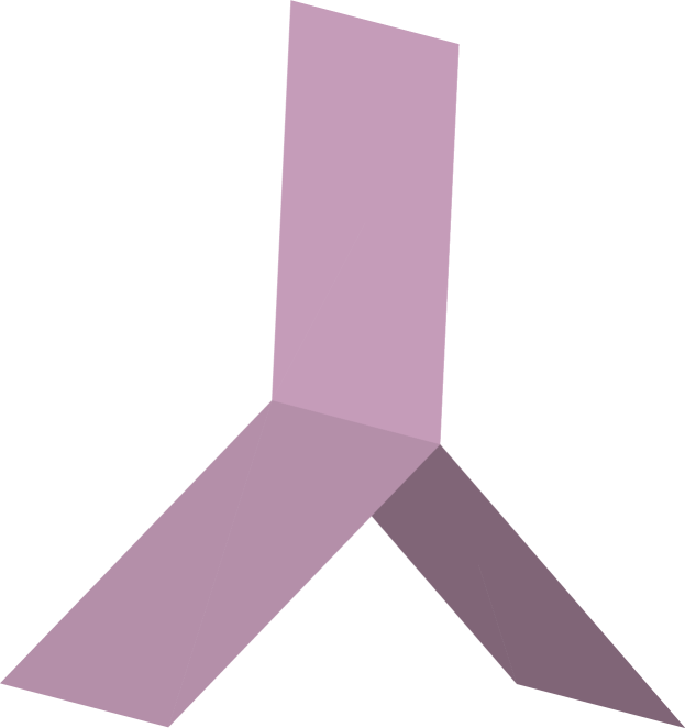
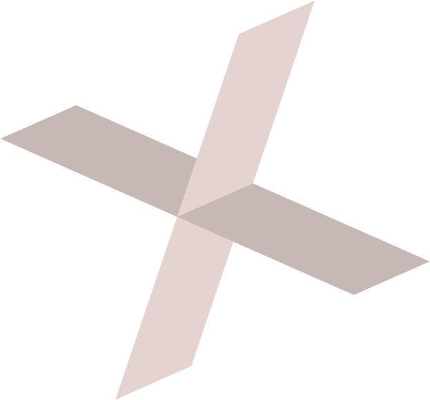
Figure 1: Two examples of multi-screen geometries

Our goal is to solve these exterior BVPs efficiently by means of Galerkin boundary element methods (BEM) [26] and Calderón preconditioning [28, 6]. For this, we recast the BVPs as variational first-kind boundary integral equations (BIEs) defined for densities on the surface of the multi-screen.

For simple screens this approach is well established [26, Section 3.5.3]. Here, we call a simple screen an orientable, piecewise smooth two-dimensional manifold with boundary $\mathcal{S}$ embedded in $\mathbb{R}^{3}$. For these geometries, the arising variational first-kind BIEs are known to be coercive [30, 16, 15] in Sobolev spaces of jumps of suitable field traces, in $\widetilde{H}^{-\frac{1}{2}}([\Gamma])$ and $\widetilde{H}^{+\frac{1}{2}}([\Gamma])$, respectively[24, Ch. 3]. For these trace spaces, conforming boundary element spaces are easily available, and they lead to Galerkin approximations and Calderón preconditioning whose numerical analysis is well-understood [25, 21, 23].

In contrast, the notion of jumps becomes problematic in multi-screens, since they are not globally orientable. For this reason, the tools from simple screens cannot be used verbatim on multi-screens. Many alternatives have been proposed to tackle this problem. [4, 31, 11, 10, 12, 13]. It is worth pointing out that at the time of writing this article, a rigorous analysis of these approaches in suitable trace spaces is not available. Furthermore, these approaches lead to ill-conditioned linear systems, yet are not amenable to preconditioning.

Fortunately, recent work by Claeys and Hiptmair offers the mathematical framework to overcome these difficulties [8]. The key idea is to see trace spaces from the perspective of quotient-spaces and to work with on multi-valued traces. This new paradigm not only allows for a rigorous analysis, but it also paves the way for conforming Galerkin discretization by means of quotient-space BEM, as proposed in [7]. Indeed, instead of trying to approximate jumps directly, the new approach relies on the Galerkin discretization of multi-trace boundary element spaces. With this approach, the related BIEs give rise to Galerkin matrices with large null spaces comprised of single-trace functions. Since the right-hand-sides of the linear systems of equations are consistent, Krylov subspace iterative solvers like GMRES still converge to the right solution. We summarize these ideas and results in Section 2.

Now that the most fundamental issues have been solved, we are in the position to investigate how to improve the computational performance of quotient-space BEM for multi-screens. Indeed, one should note that the arising linear systems are ill-conditioned and that the number of GMRES iteration counts increases with mesh refinement. Hence, a natural next step – and the main focus of this paper – is to devise preconditioners for multi-screen problems. In Section 3, we propose a simple preconditioning strategy based on opposite-order preconditioning, also known as Calderón preconditioning on closed surfaces. Moreover, we present the tools to understand the new preconditioner in the context of operator preconditioning. Numerical experiments confirm that this approach reduces considerably the number of GMRES iterations required to solve the system.

It is worth mentioning that an advantage of the quotient-space BEM approach is that minimal geometrical information is required. However, the disadvantage is that one pays with unnecessary computations due to the “doubling of degrees of freedom” underlying the discretization of multi-valued traces. As an alternative, we dedicate Section 4 to discuss reduced quotient-space representations that require slightly more geometrical information, but minimize computational effort while still rendering efficient Calderón preconditioning. Furthermore, we use the tools derived in Section 3 to provide some insight about the requirements that such reductions need to fulfil.

2 Quotient-Space Perspective

We briefly summarize the new perspective on trace spaces on multi-screens introduced in [8, Section 4-6] and the quotient-space construction of boundary element spaces from [7].

2.1 Geometry

We begin by recalling the rigorous characterization of multi-screens as given in [8, Section 2]:

Definition 1 (Lipschitz Partition [8, Definition 2.2]).

A Lipschitz partition of $\mathbb{R}^{d}$, $d=2,3$, is a finite collection of Lipschitz open sets $\left(\Omega_{j}\right)_{j=0\ldots n}$ such that $\mathbb{R}^{d}=\cup_{j=0}^{n}\overline{\Omega}_{j}$ and $\Omega_{j}\cap\Omega_{k}=\emptyset$, if $j\neq k$.

Definition 2 (Multi-screen [8, Definition 2.3]).

A multi-screen is a subset $\Gamma\subset\mathbb{R}^{d}$ such that there exists a Lipschitz partition of $\mathbb{R}^{d}$ denoted $\left(\Omega_{j}\right)_{j=0\ldots n}$ satisfying $\Gamma\subset\cup_{j=0}^{n}\partial{\Omega_{j}}$ and such that for each $j=0\ldots n$, we have $\overline{\Gamma}\cap\partial\Omega_{j}=\overline{\Gamma}_{j}$ where $\overline{\Gamma}_{j}\subset\partial\Omega_{j}$ is some Lipschitz screen in the sense of Buffa-Christiansen [2, section 1.1].

From a numerical point of view, it will be convenient to classify multi-screens into three categories. For this, we first need to consider the notion of irregular points on the boundary, as in [9].

Definition 3 (Irregular points [9, Definition 2.3]).

Let us consider $\partial\Gamma:=\Gamma\setminus\text{int}(\Gamma)$ and introduce the set of regular points of the boundary $\mathcal{P}_{R}(\partial\Gamma)$ defined as

$$\mathcal{P}_{R}(\partial\Gamma)=\{x\in\partial\Gamma\text{ such that }B_{x}\cap\Gamma=B_{x}\cap S\text{ for some ball }B_{x}\text{ centred at x and some simple Lipschitz screen }S\}.$$

We define the set of irregular points of the boundary as

$$\mathcal{P}_{I}(\partial\Gamma)=\partial\Gamma\setminus\mathcal{P}_{R}(\partial\Gamma).$$

With this, we can classify our multi-screens as follows:

• $\Gamma$ is a multi-screen such that irregular points $\mathcal{P}_{I}(\partial\Gamma)$ are on the boundary of all geometries meeting at the junction line(s).

• $\Gamma$ is a multi-screen such that irregular points $\mathcal{P}_{I}(\partial\Gamma)$ may be in the interior of at least one of the geometries meeting at the junction line(s).

• $\Gamma$ is a multi-screen without irregular points $\mathcal{P}_{I}(\partial\Gamma)$.

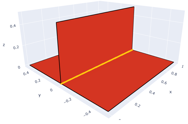
(a) Type A

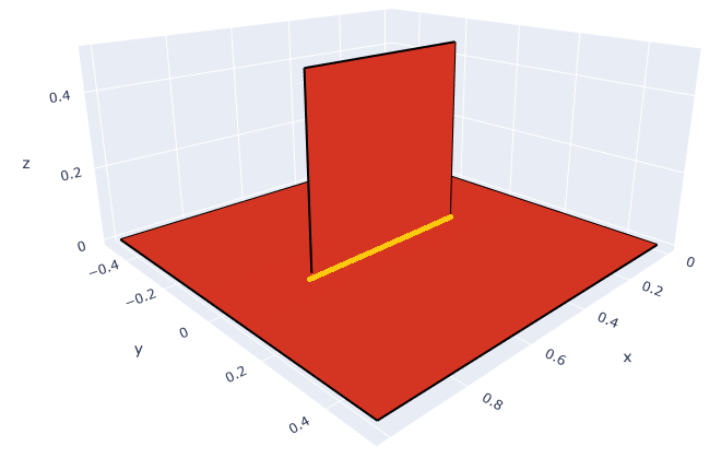
(b) Type B

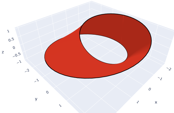
(c) Type C

Figure 2: Multi-screens can be classified according to the location of their irregular points.

Figure 2 provides examples of multi-screens in these three different classifications. Multi-screens of Type A and Type B arise from applications that we are interested in and will be the focus of this article.

2.2 Trace Spaces

Given a multi-screen $\Gamma\subset\mathbb{R}^{d}$ , with $d=2,3$, we consider the following chains of nested Sobolev spaces

$$H^{1}_{0,\Gamma}(\mathbb{R}^{d})\subset H^{1}(\mathbb{R}^{d})\subset H^{1}(\mathbb{R}^{d}\backslash\overline{\Gamma}),$$ (3a)

$$\mathbf{H}_{0,\Gamma}(\mathrm{div},\mathbb{R}^{d})\subset\mathbf{H}(\mathrm{div},\mathbb{R}^{d})\subset\mathbf{H}(\mathrm{div},\mathbb{R}^{d}\setminus\overline{\Gamma}),$$ (3b)

where a subscript $X_{0,\Gamma}$ indicates a space obtained as the closure in $X$ of smooth functions/vectorfields compactly supported in $\mathbb{R}^{d}\setminus\overline{\Gamma}$. All inclusions in (3) define closed subspaces, which describe the associated quotient-spaces Hilbert spaces. With this, we can define the multi-trace spaces [8, Section 5]

$$\mathbb{H}^{+\frac{1}{2}}(\Gamma) :=H^{1}(\mathbb{R}^{d}\backslash\overline{\Gamma})/H^{1}_{0,\Gamma}(\mathbb{R}^{d}),$$ (4a)

$$\mathbb{H}^{-\frac{1}{2}}(\Gamma) :=\mathbf{H}(\mathrm{div},\mathbb{R}^{d}\backslash\overline{\Gamma})/\mathbf{H}_{0,\Gamma}(\mathrm{div},\mathbb{R}^{d}).$$ (4b)

and the single-trace spaces [8, Section 6.1]

$$H^{+\frac{1}{2}}([\Gamma]) :=H^{1}(\mathbb{R}^{d})/H^{1}_{0,\Gamma}(\mathbb{R}^{d}),$$ (5a)

$$H^{-\frac{1}{2}}([\Gamma]) :=\mathbf{H}(\mathrm{div},\mathbb{R}^{d})/\mathbf{H}_{0,\Gamma}(\mathrm{div},\mathbb{R}^{d}).$$ (5b)

Since the spaces $H^{+\frac{1}{2}}([\Gamma])$ and $H^{-\frac{1}{2}}([\Gamma])$ are closed subspaces of $\mathbb{H}^{+\frac{1}{2}}(\Gamma)$ and $\mathbb{H}^{-\frac{1}{2}}(\Gamma)$, respectively [8, Proposition 6.2], we can also introduce the jump spaces [8, Section 6.2] as

$$\widetilde{H}^{+\frac{1}{2}}([\Gamma]):=\mathbb{H}^{+\frac{1}{2}}(\Gamma)/H^{+\frac{1}{2}}([\Gamma])\quad\text{and}\quad\widetilde{H}^{-\frac{1}{2}}([\Gamma]):=\mathbb{H}^{-\frac{1}{2}}(\Gamma)/H^{-\frac{1}{2}}([\Gamma]).$$ (6)

Remark 1.

We note that $H^{1}(\mathbb{R}^{d}\backslash\overline{\Gamma})$ and $\mathbf{H}(\mathrm{div},\mathbb{R}^{d}\setminus\overline{\Gamma})$ are spaces of functions attaining different values on both sides of $\Gamma$. This implies that functions in the multi-trace spaces $\mathbb{H}^{+\frac{1}{2}}(\Gamma)$ and $\mathbb{H}^{-\frac{1}{2}}(\Gamma)$ are multi-valued on $\Gamma$. In other words, they can take different values on both sides of $\Gamma$. One way to grasp this is to imagine an “infinitesimally inflated” screen, as illustrated in Figure 3 for a 2D multi-screen. With this, one can intuitively understand the trace spaces introduced above as follows:

• $\mathbb{H}^{+\frac{1}{2}}(\Gamma)$ can be seen as a standard Dirichlet trace space on the surface of the inflated screen. Similarly, $\mathbb{H}^{-\frac{1}{2}}(\Gamma)$ can be viewed as the standard space of Neumann trace space on the surface of the inflated screen.

• The single-trace space $H^{+\frac{1}{2}}([\Gamma])$ simply consists of single-valued functions on $\Gamma$. One can follow the same intuition for $H^{-\frac{1}{2}}([\Gamma])$, however, its right interpretation as a single-valued normal component requires that one fixes a local normal $\mathbf{n}$ on $\Gamma$.

Figure 3: Inflating a 2D multi-screen.

Next, we consider the canonical surjections

$$\pi_{D}:H^{1}(\mathbb{R}^{d}\backslash\overline{\Gamma})\rightarrow\mathbb{H}^{+\frac{1}{2}}(\Gamma)\quad\mathrm{and}\quad\pi_{N}:\mathbf{H}(\mathrm{div},\mathbb{R}^{d}\backslash\overline{\Gamma})\rightarrow\mathbb{H}^{-\frac{1}{2}}(\Gamma),$$ (7)

and $H^{1}(\Delta,\mathbb{R}^{d}\setminus\Gamma):=\{v\in H^{1}(\mathbb{R}^{d}\setminus\Gamma),\,\Delta v\in L^{2}(\mathbb{R}^{d}\setminus\Gamma)\}$. With this, we are in the position to introduce the relevant trace operators

Dirichlet trace: $$\gamma_{D}:H^{1}(\mathbb{R}^{d}\setminus\Gamma)\to\mathbb{H}^{+\frac{1}{2}}(\Gamma)\;, \gamma_{D} :=\pi_{D}\;,$$

Neumann trace: $$\gamma_{N}:H^{1}(\Delta,\mathbb{R}^{d}\setminus\Gamma)\to\mathbb{H}^{-\frac{1}{2}}(\Gamma)\;, \gamma_{N} :=\pi_{N}\circ\operatorname{\bf grad}\;.$$

Moreover, we remark that they map onto $H^{+\frac{1}{2}}([\Gamma])$ and $H^{-\frac{1}{2}}([\Gamma])$ when restricted to ${H^{1}(\mathbb{R}^{d})}$ and ${\mathbf{H}(\mathrm{div},\mathbb{R}^{d})}$, respectively.

Finally we introduce a bilinear pairing on $\mathbb{H}^{+\frac{1}{2}}(\Gamma)\times\mathbb{H}^{-\frac{1}{2}}(\Gamma)$:

$$\ll{u},{p}\gg:=\int\nolimits_{[\Gamma]}{u}{p}\ d\sigma:=\int_{\mathbb{R}^{d}\backslash\overline{\Gamma}}\mathbf{p}\cdot\nabla u+u\mathrm{div}(\mathbf{p})\ d\mathbf{x},$$ (8)

with $u\in H^{1}(\mathbb{R}^{d}\setminus\overline{\Gamma})$ and $\mathbf{p}\in\mathbf{H}(\mathrm{div},\mathbb{R}^{d}\setminus\overline{\Gamma})$ [8, Section 5.1]. Note that this pairing induces the following isometric dualities [8, Prop. 5.1 and Section 6.2]

$$\mathbb{H}^{-\frac{1}{2}}(\Gamma)\cong\left(\mathbb{H}^{+\frac{1}{2}}(\Gamma)\right)^{\prime},\quad\widetilde{H}^{-\frac{1}{2}}([\Gamma])\cong\left(H^{+\frac{1}{2}}([\Gamma])\right)^{\prime},\quad\widetilde{H}^{+\frac{1}{2}}([\Gamma])\cong\left(H^{-\frac{1}{2}}([\Gamma])\right)^{\prime}.$$ (9)

The bilinear pairing also offers a characterization of single-trace spaces through self-polarity:

Proposition 1 ([8, Proposition 6.3]).

For ${u}\in\mathbb{H}^{+\frac{1}{2}}(\Gamma)$ and ${p}\in\mathbb{H}^{-\frac{1}{2}}(\Gamma)$ the following equivalences hold true:

$${u}\in H^{+\frac{1}{2}}([\Gamma])\quad\Longleftrightarrow\quad\int_{[\Gamma]}{u}{q}\ d\sigma=0\quad\forall{q}\in H^{-\frac{1}{2}}([\Gamma]),$$

$${p}\in H^{-\frac{1}{2}}([\Gamma])\quad\Longleftrightarrow\quad\int_{[\Gamma]}{v}{p}\ d\sigma=0\quad\forall{v}\in H^{+\frac{1}{2}}([\Gamma]).$$

2.3 Weakly Singular and Hypersingular BIEs

Let

$$\mathcal{G}_{\kappa}(\mathbf{z}):=\dfrac{\exp(\imath\kappa\|\mathbf{z}\|)}{4\pi\|\mathbf{z}\|}$$

be the radiating fundamental solution of the Helmholtz equation in $\mathbb{R}^{3}$. The weakly singular boundary integral operator (BIO) can be stated in integral form as

$$(\mathsf{V}_{\kappa}{{\phi}})(\mathbf{x})=\int_{[\Gamma]}\mathcal{G}_{\kappa}(\mathbf{x}-\mathbf{y}){{\phi}}(\mathbf{y})\,d\sigma(\mathbf{y})\;,\quad{{\phi}}\in\mathbb{H}^{-\frac{1}{2}}(\Gamma)\cap\mathbb{L}^{\infty}(\Gamma),$$ (10)

where integration is carried out over the virtual inflated screen, cf. Figure 3, and $\mathbb{L}^{\infty}(\Gamma)$ is understood as the usual $L^{\infty}$ space but over the virtual inflated screen.

In order to solve the Dirichlet Helmholtz BVP, we solve the BIE given by

$${{\phi}}\in\mathbb{H}^{-\frac{1}{2}}(\Gamma):\quad\mathsf{V}_{\kappa}({{\phi}})={{g}}_{D},$$ (11)

which can be written in equivalent variational form as follows:

$$\mathrm{Find\ }{{\phi}}\in\mathbb{H}^{-\frac{1}{2}}(\Gamma)\ \mathrm{such\ that}\quad\ll\mathsf{V}_{\kappa}{{\phi}},{{\psi}}\gg=\ll{{g}_{D}},{{\psi}}\gg\quad\forall{{\psi}}\in\mathbb{H}^{-\frac{1}{2}}(\Gamma).$$ (12)

Similarly, solving the Neumann Helmholtz BVP is equivalent to solving the BIE

$${{v}}\in\mathbb{H}^{+\frac{1}{2}}(\Gamma):\quad\mathsf{W}_{\kappa}({{v}})={{f}}_{N}.$$ (13)

Also this BIE can be cast in variational form and this results in the problem:

$$\mathrm{Find\ }{{v}}\in\mathbb{H}^{+\frac{1}{2}}(\Gamma)\ \mathrm{such\ that}\quad\ll\mathsf{W}_{\kappa}{{v}},{{p}}\gg=\ll{{f}_{N}},{{p}}\gg\quad\forall{{p}}\in\mathbb{H}^{+\frac{1}{2}}(\Gamma).$$ (14)

As shown in [26, Section 3.3], the bilinear form on the left-hand side of (14) can be conveniently expressed by integration by parts over the virtual inflated screen for sufficiently regular arguments:

$$\begin{aligned} \ll\mathsf{W}_{\kappa}{{v}},{{p}}\gg=\int_{[\Gamma]}\int_{[\Gamma]}G_{\kappa}(\mathbf{y}-\mathbf{x})\Bigl{\{}&(\operatorname{\bf grad}_{\Gamma}{{v}}\times\mathbf{n})(\mathbf{y})\cdot(\operatorname{\bf grad}_{\Gamma}{{p}}\times\mathbf{n})(\mathbf{x})\\ &-\kappa^{2}\mathbf{n}(\mathbf{y})\cdot\mathbf{n}(\mathbf{x}){{v}}(\mathbf{y}){{p}}(\mathbf{x})\Bigr{\}}\,d\sigma(\mathbf{y})d\sigma(\mathbf{x}).\end{aligned}$$ (15)

We conclude this section by reminding the reader of some properties of these BIEs:

Proposition 2 ( [8, Prop. 8.8]).

There exist compact operators $\mathsf{K}_{V}:\widetilde{H}^{-\frac{1}{2}}([\Gamma])\rightarrow H^{+\frac{1}{2}}([\Gamma])$ and $\mathsf{K}_{W}:\widetilde{H}^{+\frac{1}{2}}([\Gamma])\rightarrow H^{-\frac{1}{2}}([\Gamma])$ such that the following Gårding inequalities are satisfied

$$\mathrm{Re}\left\{\int_{[\Gamma]}{{q}}(\mathsf{V}_{\kappa}+\mathsf{K}_{V})\bar{{{q}}}\ d\sigma\right\} \geq C_{\mathsf{V}}\lVert{{q}}\rVert^{2}_{\widetilde{H}^{-\frac{1}{2}}([\Gamma])}\quad\forall{{q}}\in\widetilde{H}^{-\frac{1}{2}}([\Gamma]),$$ (16)

$$\mathrm{Re}\left\{\int_{[\Gamma]}{{v}}(\mathsf{W}_{\kappa}+\mathsf{K}_{W})\bar{{{v}}}\ d\sigma\right\} \geq C_{\mathsf{W}}\lVert{{v}}\rVert^{2}_{\widetilde{H}^{+\frac{1}{2}}([\Gamma])}\quad\forall{{v}}\in\widetilde{H}^{+\frac{1}{2}}([\Gamma]),$$ (17)

with $C_{\mathsf{V}},C_{\mathsf{W}}>0$ depending only on $\kappa$ and $\Gamma$.

Lemma 1 ([7, Lemma 3.2]).

The nullspaces of ${\mathsf{V}_{\kappa}}$ and ${\mathsf{W}_{\kappa}}$ agree with ${H^{-\frac{1}{2}}([\Gamma])}$ and $H^{+\frac{1}{2}}([\Gamma])$, respectively.

From these results, we see that ${\mathsf{V}_{\kappa}}$ and ${\mathsf{W}_{\kappa}}$ remain well-defined on the corresponding jump spaces and are coercive there. Indeed, Theorem 8.11 in [29] combined with [8, Prop. 8.8] and [8, Prop. 8.9] gives us the following inf-sup conditions:

Corollary 1.

1. For a dense sequence of finite dimensional subspaces $(\widetilde{Z}^{1/2}_{h}(\Gamma))_{h\in\mathcal{H}}\subset\widetilde{H}^{+\frac{1}{2}}([\Gamma])$ there exist $h_{0}>0$ such that for all $h\leq h_{0}$ it holds

   $$\underset{u_{h}\in\widetilde{Z}^{1/2}_{h}(\Gamma)}{\inf}\>\underset{v_{h}\in\widetilde{Z}^{1/2}_{h}(\Gamma)}{\sup}\dfrac{|\langle\mathsf{W}_{\kappa}u_{h},v_{h}\rangle|}{\|u_{h}\|_{\widetilde{H}^{+\frac{1}{2}}([\Gamma])}\|v_{h}\|_{\widetilde{H}^{+\frac{1}{2}}([\Gamma])}}\geq\alpha_{\mathsf{W}_{\kappa}}>0,$$ (18)

   and

   $$\underset{v_{h}\in\widetilde{Z}^{1/2}_{h}(\Gamma)}{\inf}\>\underset{u_{h}\in\widetilde{Z}^{1/2}_{h}(\Gamma)}{\sup}\dfrac{|\langle\mathsf{W}_{\kappa}u_{h},v_{h}\rangle|}{\|u_{h}\|_{\widetilde{H}^{+\frac{1}{2}}([\Gamma])}\|v_{h}\|_{\widetilde{H}^{+\frac{1}{2}}([\Gamma])}}\geq\alpha_{\mathsf{W}_{\kappa}}>0,$$ (19)

   where $\alpha_{\mathsf{W}_{\kappa}}$ is independent of $h$.

2. For a dense sequence of finite dimensional subspaces $(\widetilde{Z}^{-1/2}_{h}(\Gamma))_{h\in\mathcal{H}}\subset\widetilde{H}^{-\frac{1}{2}}([\Gamma])$ there exist $h_{0}>0$ such that for all $h\leq h_{0}$ it holds

   $$\underset{\mu_{h}\in\widetilde{Z}^{-1/2}_{h}(\Gamma)}{\inf}\>\underset{\varphi_{h}\in\widetilde{Z}^{-1/2}_{h}(\Gamma)}{\sup}\dfrac{|\langle\mathsf{V}_{\kappa}\mu_{h},\varphi_{h}\rangle|}{\|\mu_{h}\|_{\widetilde{H}^{-\frac{1}{2}}([\Gamma])}\|\varphi_{h}\|_{\widetilde{H}^{-\frac{1}{2}}([\Gamma])}}\geq\alpha_{\mathsf{V}_{\kappa}}>0,$$ (20)

   and

   $$\underset{\varphi_{h}\in\widetilde{Z}^{-1/2}_{h}(\Gamma)}{\inf}\>\underset{\mu_{h}\in\widetilde{Z}^{-1/2}_{h}(\Gamma)}{\sup}\dfrac{|\langle\mathsf{V}_{\kappa}\mu_{h},\varphi_{h}\rangle|}{\|\mu_{h}\|_{\widetilde{H}^{-\frac{1}{2}}([\Gamma])}\|\varphi_{h}\|_{\widetilde{H}^{-\frac{1}{2}}([\Gamma])}}\geq\alpha_{\mathsf{V}_{\kappa}}>0,$$ (21)

   where $\alpha_{\mathsf{V}_{\kappa}}$ is independent of $h$.

Additionally, these operators are also well-defined on the multi-trace spaces $\mathbb{H}^{-\frac{1}{2}}(\Gamma)$ and $\mathbb{H}^{+\frac{1}{2}}(\Gamma)$, respectively. However, Lemma 1 implies that they have non-trivial nullspaces when considered on multi-trace spaces. Although this hinders uniqueness of solutions for (12) and (14), Proposition 1 still provides existence, since ${g}_{D}\in H^{+\frac{1}{2}}([\Gamma])$ and ${f}_{N}\in H^{-\frac{1}{2}}([\Gamma])$ guarantees consistency of the right-hand side linear forms: they vanish on the single-trace spaces.

3 Calderón Preconditioning for Quotient-Space BEM

As already mentioned in the introduction, the linear systems arising from the discretization of (12) and (14) using Quotient-space BEM are ill-conditioned, which causes that the number of GMRES iteration counts increases with mesh refinement. One should note that this is not a particularity of Quotient-space BEM. Indeed, we usually encounter this difficulty when using low-order BEM discretization of first-kind integral equations on simple screens and closed surfaces. In those cases, one typically fixes the problem by using so-called Calderón preconditioning, which combines Calderón identities with operator preconditioning to build a very convenient and effective preconditioner [28, 6, 20].

In this paper, we will extend this approach and devise Calderón preconditioners for the problem at hand. Following the policy of operator preconditioning (see, for instance [20]), we introduce the following more general notation in order to state the results that will hold for both BIEs under consideration (i.e. (11) and (13)):

• Let $\mathbb{X}(\Gamma)$ and $\mathbb{Y}(\Gamma)$ be multi-trace spaces such that $\mathbb{Y}(\Gamma)=\left(\mathbb{X}(\Gamma)\right)^{\prime}$.

• Let $X(\Gamma)$ and $Y(\Gamma)$ be single-trace spaces such that $X(\Gamma)\subset\mathbb{X}(\Gamma)$ and $Y(\Gamma)\subset\mathbb{Y}(\Gamma)$.

• Let $\widetilde{X}(\Gamma)$ and $\widetilde{Y}(\Gamma)$ be jump spaces such that $\widetilde{X}(\Gamma)=\mathbb{X}(\Gamma)/X(\Gamma)$ and $\widetilde{Y}(\Gamma)=\mathbb{Y}(\Gamma)/Y(\Gamma)$.

What these spaces will be exactly, depends on whether we are solving the Dirichlet or Neumann problem. For clarity, we will consider each case separately in the next Subsections.

Now, in both cases, we are interested in continuous sesquilinear forms $\mathsf{a}\in L(\mathbb{X}(\Gamma)\times\mathbb{X}(\Gamma),\mathbb{C})$, that will characterize the variational formulations of our BIEs (12) and (14). However, unlike in the traditional operator preconditioning setting [20], we know from Corollary 1 that these sesquilinear forms $\mathsf{a}$ will satisfy an inf-sup condition on $\widetilde{X}(\Gamma)$, but not on $\mathbb{X}(\Gamma)$.

Naturally, this will affect the corresponding discrete inf-sup conditions, and hence, the condition number bounds. The remainder of this section is dedicated to understanding this, and to answering the question of whether the discrete inf-sup conditions are satisfied and how they depend on the mesh parameter $h$ when using Quotient-space BEM.

Let us begin by introducing the notation for the corresponding finite dimensional spaces. On the one hand, we will work with

• $\mathbb{X}_{h}(\Gamma)\subset\mathbb{X}(\Gamma)$ : primal multi-trace BE space for $\Gamma$; and

• $\mathbb{Y}_{h}(\Gamma)\subset\mathbb{Y}(\Gamma)$ : dual multi-trace BE space for $\Gamma$,

which will be actually used for the implementation. We remark that $\mathbb{X}_{h}(\Gamma)$ and $\mathbb{Y}_{h}(\Gamma)$ are Hilbert spaces. On the other hand, we consider the finite-dimensional subspaces

$$X_{h}(\Gamma)\subset X(\Gamma),\qquad Y_{h}(\Gamma)\subset Y(\Gamma),$$

$$\widetilde{X}_{h}(\Gamma)\subset\widetilde{X}(\Gamma),\qquad\widetilde{Y}_{h}(\Gamma)\subset\widetilde{Y}(\Gamma),$$

which will only be used to show our theoretical results. It is worth mentioning that we always assume that these finite-dimensional subspaces satisfy

$$X_{h}(\Gamma) \subset\mathbb{X}_{h}(\Gamma), \quad Y_{h}(\Gamma) \subset\mathbb{Y}_{h}(\Gamma),$$

$$\widetilde{X}_{h}(\Gamma) =\mathbb{X}_{h}(\Gamma)/X_{h}(\Gamma), \quad\widetilde{Y}_{h}(\Gamma) =\mathbb{Y}_{h}(\Gamma)/Y_{h}(\Gamma).$$

3.1 Preconditioning the Hypersingular operator

When considering the Neumann problem (14), we will have that $\mathbb{X}(\Gamma)=\mathbb{H}^{+\frac{1}{2}}(\Gamma)$, $X(\Gamma)=H^{+\frac{1}{2}}([\Gamma])$, $\widetilde{X}(\Gamma)=\widetilde{H}^{+\frac{1}{2}}([\Gamma])$ for primal spaces, and $\mathbb{Y}(\Gamma)=\mathbb{H}^{-\frac{1}{2}}(\Gamma)$, $Y(\Gamma)=H^{-\frac{1}{2}}([\Gamma])$, $\widetilde{Y}(\Gamma)=\widetilde{H}^{-\frac{1}{2}}([\Gamma])$ for dual ones.

Let $\mathcal{T}_{h}$ be a triangular virtual surface mesh of $\Gamma$ built as in [7, Section 4.1], with target element size $h$, and let $\check{\mathcal{T}}_{h}$ be its dual as realised on the barycentric refinement [3]. It is worth noticing that the BE spaces above can be chosen as

• $\mathbb{X}_{h}(\Gamma)=\mathcal{S}^{1,0}(\mathcal{T}_{h})$: piecewise linear “continuous” functions on $\mathcal{T}_{h}$,

• $\mathbb{Y}_{h}(\Gamma)=\mathcal{S}^{0,-1}(\check{\mathcal{T}}_{h})$: piecewise constant functions on $\check{\mathcal{T}}_{h}$,

Moreover, the duality pairing $\ll\cdot,\cdot\gg$ preserves the duality $\mathbb{Y}_{h}(\Gamma)=\left(\mathbb{X}_{h}(\Gamma)\right)^{\prime}$.

3.1.1 A flawed idea

With these choices and Corollary 1, we have that

$$\sup_{\mu_{h}\in Y_{h}(\Gamma)}\dfrac{|\ll x_{h},\mu_{h}\gg|}{\|\mu_{h}\|_{H^{-\frac{1}{2}}([\Gamma])}}\geq C_{1}\|x_{h}\|_{\widetilde{H}^{+\frac{1}{2}}([\Gamma])},\qquad\text{ and}\qquad\sup_{u_{h}\in\widetilde{X}_{h}(\Gamma)}\dfrac{|\ll\mathsf{W}_{\kappa}\,x_{h},u_{h}\gg|}{\|u_{h}\|_{\widetilde{H}^{+\frac{1}{2}}([\Gamma])}}\geq C_{\mathsf{W}}\|x_{h}\|_{\widetilde{H}^{+\frac{1}{2}}([\Gamma])},$$ (22)

for all $x_{h}\in\widetilde{X}_{h}(\Gamma)$. Therefore, it only remains to find an operator $\mathsf{B}_{\kappa}:H^{-\frac{1}{2}}([\Gamma])\to\widetilde{H}^{+\frac{1}{2}}([\Gamma])$ such that

$$\sup_{\mu_{h}\in Y_{h}(\Gamma)}\dfrac{|\ll\mathsf{B}_{\kappa}\,y_{h},\mu_{h}\gg|}{\|\mu_{h}\|_{H^{-\frac{1}{2}}([\Gamma])}}\geq C_{\mathsf{B}}\|y_{h}\|_{H^{-\frac{1}{2}}([\Gamma])},\quad\forall y_{h}\in Y_{h}(\Gamma).$$ (23)

Furthermore, based on Calderón preconditioning for closed surfaces and its applicability to simple screens, one could think of setting $\mathsf{B}_{\kappa}$ to be the weakly singular operator $\mathsf{V}_{\kappa}$. However, it is clear from Lemma 1 that $\mathsf{V}_{\kappa}$ will not do the job.

3.1.2 Changing perspective

In order to find the right operator $\mathsf{B}_{\kappa}$, it is useful to first understand what we are looking for. Indeed, when pursuing a quotient-space discretization $\widetilde{X}_{h}(\Gamma)$ of $\widetilde{H}^{+\frac{1}{2}}([\Gamma])$, it makes sense to study the Galerkin matrices in the multi-trace discrete spaces $\mathbb{X}_{h}(\Gamma)$ and $\mathbb{Y}_{h}(\Gamma)$.

Let $\mathbf{A}_{\mathsf{W}}$ be the Galerkin matrix of the hypersingular operator $\mathsf{W}_{\kappa}$ on $\mathbb{X}_{h}(\Gamma)$. Then we know from Lemma 1 and [7] that $\ker(\mathbf{A}_{\mathsf{W}})=X_{h}(\Gamma)$ and that GMRES can still solve the arising linear system as long as the right hand side vector $\mathbf{g}$ is consistent, i.e. $\mathbf{g}\in\text{Range}(\mathbf{A}_{\mathsf{W}})$.

Let $\mathbf{P}_{\mathsf{W}}$ be the matrix we will use to (left) precondition $\mathbf{A}_{\mathsf{W}}$. The first condition we need to satisfy is that the system

$$\mathbf{P}_{\mathsf{W}}\mathbf{A}_{\mathsf{W}}\mathbf{u}=\mathbf{P}_{\mathsf{W}}\mathbf{g}$$ (24)

is consistent. If we choose $\mathbf{P}_{\mathsf{W}}$ to be invertible, this is automatically satisfied. Hence, in order to have a suitable operator preconditioner we need

• a stable duality pairing for $\mathbb{X}_{h}(\Gamma)\times\mathbb{Y}_{h}(\Gamma)$; and

• $\mathbf{B}_{\kappa,h}$ invertible (in $\mathbb{Y}_{h}(\Gamma)$),

since this will imply that $\mathbf{P}_{\mathsf{W}}=\mathbf{M}^{-1}\mathbf{B}_{\kappa,h}\mathbf{M}^{-T}$ is invertible. Here $\mathbf{M}$ is the Galerkin matrix of the duality pairing $\mathbb{X}_{h}(\Gamma)\times\mathbb{Y}_{h}(\Gamma)$.

3.1.3 Implementation

Note that by construction of the inflated screen, which can be understood as a virtual closed surface, the space $\mathcal{S}^{1,0}(\mathcal{T}_{h})$ has one degree of freedom at the vertices in $\mathcal{T}_{h}\cap\partial\Gamma$. Since solutions for the hypersingular equation (14) live in $\widetilde{H}^{+\frac{1}{2}}([\Gamma])$, we know they will be zero on $\partial\Gamma$ [7]. Considering that solutions for the hypersingular equation (14) live in $\widetilde{H}^{+\frac{1}{2}}([\Gamma])$, and because such functions are only determined up to contributions in $H^{+\frac{1}{2}}([\Gamma])$, degrees of freedom on $\partial\Gamma$ (which by construction are in $H^{+\frac{1}{2}}([\Gamma])$) can be safely deleted. Hence, instead of working with $\mathcal{S}^{1,0}(\mathcal{T}_{h})$, we consider $\mathcal{S}_{0}^{1,0}(\mathcal{T}_{h})\subset\mathbb{H}^{+\frac{1}{2}}(\Gamma)$ : piecewise linear “continuous” functions on the inflated screen $[\Gamma]$ that are zero on $\partial\Gamma$.

When dealing with multi-screens of type A, this will have the computational advantage of allowing us to decouple the BE spaces on each side of the triangular virtual surface mesh $\mathcal{T}_{h}$, as depicted in Figure 4.

Let us illustrate how we implemented these BE spaces on a multi-screen $\Gamma$ that consists of three simple screens $\Gamma_{i},i=1,2,3$ meeting at a junction:

1. We decompose the inflated multi-screen $[\Gamma]$ as

   $$[\Gamma]=\cup_{l=1}^{3}\mathcal{I}_{l}$$ (25)

   with $\mathcal{I}_{l}=\Gamma_{l}\cup\Gamma_{l+1}$. The normal on $\mathcal{I}_{l}$ is chosen outward. Each simple screen $\Gamma_{i}$ appears once as the front and once as the back of the multi-screen (Figure 4).

2. For $i=1,2,3$, we create the triangular surface mesh $\Gamma_{i,h}$ of $\Gamma_{i}$ with target element size $h$, and such that the meshes $\Gamma_{i,h}$ for $i=1,2,3$ match up along the junction.

   We remark that the simple screens $\mathcal{I}_{l}$ inherit this mesh. In other words, we have $\mathcal{I}_{l,h}=\Gamma_{l,h}\bigcup\Gamma_{l+1,h},\,l=1,2,3$.

   

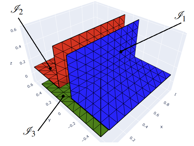
   Figure 4: Back-front conforming mesh on the multi-screen.

3. The discrete primal multi-trace space is built as the direct product of these spaces, i.e.

   $$\mathbb{X}_{h}(\Gamma)=\mathcal{S}_{0}^{1,0}(\mathcal{T}_{h})=\prod_{l=1}^{3}\mathcal{S}_{0}^{1,0}(\mathcal{I}_{l,h}).$$ (26)

4. Construct the dual BE spaces on the simple screens $\mathcal{I}_{l}$ following the cue from [3]. For this, let $\check{\mathcal{I}}_{l,h}$ denote the dual barycentric mesh to $\mathcal{I}_{l,h}$, built as in [22, Definition 2]. Then we introduce the space $\mathcal{S}^{0,-1}(\check{\mathcal{I}}_{l,h})\subset\mathbb{H}^{-\frac{1}{2}}(\mathcal{I}_{l})$ of piecewise constant functions supported by the dual cells of $\check{\mathcal{I}}_{l,h}$ that correspond to nodes not on the boundary of $\mathcal{I}_{l}$. In particular we have that $\dim\mathcal{S}^{0,-1}(\check{\mathcal{I}}_{l,h})=\dim\mathcal{S}^{1,0}_{0}(\mathcal{I}_{l,h})$.

5. The discrete dual multi-trace space is built as the direct product of these dual spaces, i.e.

   $$\mathbb{Y}_{h}(\Gamma)=\mathcal{S}^{0,-1}(\check{\mathcal{T}}_{h})=\prod_{l=1}^{3}\mathcal{S}^{0,-1}(\check{\mathcal{I}}_{l,h}).$$ (27)

Remark 2.

It is worth noticing that the $L^{2}(\Gamma)$-duality product between $\mathbb{X}_{h}(\Gamma)$ and $\mathbb{Y}_{h}(\Gamma)$ as chosen in (26) and (27) is stable [27]. Hence, this implementation leads to a Galerkin matrix $\mathbf{M}$ that is bounded and invertible.

Remark 3.

The description of discrete multi-trace spaces (26) and (27) is not valid for multi-screens of Types B and C.

3.1.4 Block Calderón Preconditioner

Under the considerations of the previous subsections, we propose to use Calderón preconditioning blockwise. This means, we will build a preconditioner for the Galerkin matrix for the hypersingular operator $\mathbf{W}_{\kappa,h}$ based on the dual Galerkin matrix

$$\mathbf{B}_{\kappa,h}^{\mathsf{V}}:=\left(\begin{array}[]{c c c}\check{\mathbf{V}}_{\kappa,1}&\mathbf{0}&\mathbf{0}\\ \mathbf{0}&\check{\mathbf{V}}_{\kappa,2}&\mathbf{0}\\ \mathbf{0}&\mathbf{0}&\check{\mathbf{V}}_{\kappa,3}\\ \end{array}\right),$$ (31)

where $\check{\mathbf{V}}_{\kappa,l}[i,j]=\langle\mathsf{V}_{\kappa}\check{\psi}_{j},\check{\psi}_{i}\rangle_{\mathcal{I}_{l}}$ with $\check{\psi}_{i},\check{\psi}_{j}$ in the standard basis of $\mathcal{S}^{0,-1}(\check{\mathcal{I}}_{l,h})$ for $l=1,2,3$.

The motivation to consider this $\mathbf{B}_{\kappa,h}^{\mathsf{V}}$ is that the choice of discrete spaces from (26) and (27) allows us to decouple what is happening on the dual space of each simple screen $\mathcal{I}_{l}$. Furthermore, they would agree with the standard discretization of the jump spaces on simple screens. More concretely, we have that $\mathcal{S}_{0}^{1,0}({\mathcal{I}}_{l,h})\subset\widetilde{H}^{1/2}(\mathcal{I}_{l})$ and $\mathcal{S}^{0,-1}(\check{\mathcal{I}}_{l,h})\subset\widetilde{H}^{-1/2}(\mathcal{I}_{l})$.

Proposition 3.

Let $\mathsf{B}_{\kappa,h}^{\mathsf{V}}\,:\,\mathbb{Y}_{h}(\Gamma)\to\mathbb{X}_{h}(\Gamma)$ be the linear operator corresponding to $\mathbf{B}_{\kappa,h}^{\mathsf{V}}$ defined in (31). For the discrete spaces defined in this Subsection, we have that for all $h\leq h_{0}$ it holds that

$$\sup_{u_{h}\in\mathbb{Y}_{h}(\Gamma)\setminus\{0\}}\dfrac{|\ll\mathsf{B}_{\kappa,h}^{\mathsf{V}}v_{h},u_{h}\gg|}{\|u_{h}\|_{\mathbb{H}^{+\frac{1}{2}}(\Gamma)}}\geq\alpha_{\mathsf{B}_{\mathsf{V}}}(1+|\log h|)^{-2}\|v_{h}\|_{\mathbb{H}^{+\frac{1}{2}}(\Gamma)}$$ (32)

for all $v_{h}\in\mathbb{H}^{+\frac{1}{2}}(\Gamma)$, and with $\alpha_{\mathsf{B}_{\mathsf{V}}}>0$ independent of $h$.

Proof.

By definition of $\mathbf{B}_{\kappa,h}^{\mathsf{V}}$ we have that

$$\sup_{u_{h}\in\mathbb{Y}_{h}(\Gamma)\setminus\{0\}}\dfrac{|\ll\mathsf{B}_{\kappa,h}^{\mathsf{V}}v_{h},u_{h}\gg|}{\|u_{h}\|_{\mathbb{H}^{+\frac{1}{2}}(\Gamma)}}=\sup_{u_{h}\in\mathbb{Y}_{h}(\Gamma)\setminus\{0\}}\dfrac{|\sum_{l}\langle\mathsf{W}_{\kappa}v_{h},u_{h}\rangle_{\mathcal{I}_{l}}|}{\|u_{h}\|_{\mathbb{H}^{+\frac{1}{2}}(\Gamma)}}.$$ (33)

Recall that $\mathsf{W}_{\kappa}$ satisfies a Gårding inequality on each $\mathcal{I}_{l}$ with a compact operator $\mathsf{T}_{\mathsf{W},l}$. Let $\mathsf{D}_{\mathsf{W},l}:=\mathsf{W}_{\kappa}+\mathsf{T}_{\mathsf{W},l}$ and denote by $u_{hl}$ the restriction of $u_{h}$ to $\mathcal{I}_{l}$. Then, we choose $u_{h}$ such that $u_{hl}=v_{hl}-{\mathsf{D}_{\mathsf{W},l}}^{-1}\mathsf{T}_{\mathsf{W},l}v_{hl}$. Plugging this into (33) gives

$$\sup_{u_{h}\in\mathbb{Y}_{h}(\Gamma)\setminus\{0\}}\dfrac{|\ll\mathsf{B}_{\kappa,h}^{\mathsf{V}}v_{h},u_{h}\gg|}{\|u_{h}\|_{\mathbb{H}^{+\frac{1}{2}}(\Gamma)}}\geq\dfrac{|\sum_{l}\langle\mathsf{W}_{\kappa}v_{hl},v_{hl}-{\mathsf{D}_{\mathsf{W},l}}^{-1}\mathsf{T}_{\mathsf{W},l}v_{hl}\rangle_{\mathcal{I}_{l}}|}{\|u_{h}\|_{\mathbb{H}^{+\frac{1}{2}}(\Gamma)}}$$ (34)

Next, following standard arguments (c.f[29, Theorem 8.11]), one gets that for this choices of $u_{hl}$ there exists an $\tilde{h}_{l}\in\mathbb{R}_{+}$ such that

$$\langle\mathsf{W}_{\kappa}v_{hl},u_{hl}\rangle_{\mathcal{I}_{l}}\geq\tilde{c}_{l}\|v_{hl}\|_{\widetilde{H}^{1/2}(\mathcal{I}_{l})}\|u_{hl}\|_{\widetilde{H}^{1/2}(\mathcal{I}_{l})}\geq\tilde{c}_{l}\|v_{hl}\|_{{H}^{1/2}(\mathcal{I}_{l})}\|u_{hl}\|_{{H}^{1/2}(\mathcal{I}_{l})}$$

is satisfied for all $h\leq\tilde{h}_{l}$, and with $\tilde{c}_{l}>0$ independent of $h$. Hence, we get

$$\sup_{u_{h}\in\mathbb{Y}_{h}(\Gamma)\setminus\{0\}}\dfrac{|\ll\mathsf{B}_{\kappa,h}^{\mathsf{V}}v_{h},u_{h}\gg|}{\|u_{h}\|_{\mathbb{H}^{+\frac{1}{2}}(\Gamma)}}\geq\dfrac{\sum_{l}\tilde{c}_{l}\|v_{hl}\|_{{H}^{1/2}(\mathcal{I}_{l})}\|u_{hl}\|_{{H}^{1/2}(\mathcal{I}_{l})}}{\|u_{h}\|_{\mathbb{H}^{+\frac{1}{2}}(\Gamma)}},$$ (35)

for all $h\leq h_{0}:=\min_{l}\tilde{h}_{l}$.

Now, let $c_{*}=\min\tilde{c}_{l}$ and use Polya and Szegö’s inequality to further bound our expression as follows

$$\sup_{u_{h}\in\mathbb{Y}_{h}(\Gamma)\setminus\{0\}}\dfrac{|\ll\mathsf{B}_{\kappa,h}^{\mathsf{V}}v_{h},u_{h}\gg|}{\|u_{h}\|_{\mathbb{H}^{+\frac{1}{2}}(\Gamma)}}\geq c_{*}\dfrac{\sum_{l_{1}}\|v_{hl_{1}}\|_{{H}^{1/2}(\mathcal{I}_{l_{1}})}\sum_{l_{2}}\|u_{hl_{2}}\|_{{H}^{1/2}(\mathcal{I}_{l_{2}})}}{\|u_{h}\|_{\mathbb{H}^{+\frac{1}{2}}(\Gamma)}}.$$ (36)

Finally, using the inverse inequality from Lemma 8, we conclude

$$\sup_{u_{h}\in\mathbb{Y}_{h}(\Gamma)\setminus\{0\}}\dfrac{|\ll\mathsf{B}_{\kappa,h}^{\mathsf{V}}v_{h},u_{h}\gg|}{\|u_{h}\|_{\mathbb{H}^{+\frac{1}{2}}(\Gamma)}}\geq\tilde{c}_{*}(1+|\log h|)^{-2}\|v_{h}\|_{\mathbb{H}^{+\frac{1}{2}}(\Gamma)}.$$ (37)

∎

3.1.5 Condition number estimates

Although GMRES convergence estimates do not rely only on spectral condition numbers, it is often a useful piece of information in the context of operator preconditioning because it gives us a simple criteria to preserve stability, study asymptotic behaviours and to compare our preconditioning results with what is known in the literature for simple screens. Moreover, as we will see later, it will help us provide criteria to choose smaller discrete spaces that are still amenable to efficient preconditioning.

Theorem 1.

Let $\mathbf{W}_{\kappa,h}$ be the Galerkin matrix corresponding to $\mathsf{W}_{\kappa}$ discretized over $\mathbb{X}_{h}(\Gamma)\subset\mathbb{H}^{+\frac{1}{2}}(\Gamma)$, and $\mathbf{M}$ the Galerkin matrix of the duality pairing for $\mathbb{X}_{h}(\Gamma)\times\mathbb{Y}_{h}(\Gamma)$ as chosen above.

Assume that there exists an operator $\mathsf{R}_{h}^{+}\,:\,\mathbb{H}^{+\frac{1}{2}}(\Gamma)\to\mathbb{X}_{h}(\Gamma)$ such that

• $\mathsf{R}_{h}^{+}$ is a h-uniformly bounded projection

• $\mathsf{R}_{h}^{+}(H^{+\frac{1}{2}}([\Gamma]))\subseteq X_{h}(\Gamma).$

Then, under the mesh conditions from Assumption 2, we have

$$\kappa_{sp}(\mathbf{M}^{-1}\mathbf{B}_{\kappa,h}^{\mathsf{V}}\mathbf{M}^{-T}\mathbf{W}_{\kappa,h})\leq(1+|\log h|)^{2}\dfrac{\alpha_{\mathsf{M}}^{2}\|\mathsf{W}_{\kappa}\|\|\mathsf{V}_{\kappa}\|}{\|\mathsf{M}\|^{2}\alpha_{\mathsf{B}}\alpha_{\mathsf{a}}},$$ (38)

where $\|\|$ denotes operator norms and $\alpha_{(}\cdot)$ corresponding inf-sup constants.

Proof.

Given the inf-sup constants from Corollary 1 and Proposition 3, and the norm equivalences from Lemmas 9 and 10 shown in Appendix A.2, the result follows from the derivation in Appendix A.3. ∎

3.2 Preconditioning the Weakly singular operator

Now we are interested in the Dirichlet variational problem (12), where we have $\mathbb{X}(\Gamma)=\mathbb{H}^{-\frac{1}{2}}(\Gamma)$, $X(\Gamma)=H^{-\frac{1}{2}}([\Gamma])$, and $\widetilde{X}(\Gamma)=\widetilde{H}^{-\frac{1}{2}}([\Gamma])$ for the primal spaces; and $\mathbb{Y}(\Gamma)=\mathbb{H}^{+\frac{1}{2}}(\Gamma)$, $Y(\Gamma)=H^{+\frac{1}{2}}([\Gamma])$, and $\widetilde{Y}(\Gamma)=\widetilde{H}^{+\frac{1}{2}}([\Gamma])$ for the dual ones.

This time, we chose these BE spaces as

• $\mathbb{X}_{h}(\Gamma)=\mathcal{S}^{0,-1}(\mathcal{T}_{h})$: piecewise constant functions on $\mathcal{T}_{h}$,

• $\mathbb{Y}_{h}(\Gamma)=\mathcal{S}^{1,0}(\check{\mathcal{T}}_{h})$: the piecewise linear, continuous functions on $\check{\mathcal{T}}_{h}$ as built in [3],

Moreover, the duality pairing $\ll\cdot,\cdot\gg$ preserves the duality $\mathbb{Y}_{h}(\Gamma)=\left(\mathbb{X}_{h}(\Gamma)\right)^{\prime}$.

In analogy to what we discussed in subsection 3.1, we have that standard Calderón preconditioning, i.e. using $\mathsf{W}_{\kappa}$ to precondition $\mathsf{V}_{\kappa}$ will not work. Hence, we will again consider a block diagonal Calderón preconditioner:

$$\mathbf{B}_{\kappa,h}^{\mathsf{W}}:=\left(\begin{array}[]{c c c}\check{\mathbf{W}}_{\kappa,1}&\mathbf{0}&\mathbf{0}\\ \mathbf{0}&\check{\mathbf{W}}_{\kappa,2}&\mathbf{0}\\ \mathbf{0}&\mathbf{0}&\check{\mathbf{W}}_{\kappa,3}\\ \end{array}\right),$$ (42)

where $\check{\mathbf{W}}_{\kappa,l}[i,j]=\langle\mathsf{W}_{\kappa}\check{\psi}_{j},\check{\psi}_{i}\rangle_{\mathcal{I}_{l}}$ with $\check{\varphi}_{i},\check{\varphi}_{j}$ in the standard basis for $\mathcal{S}^{1,0}(\check{\mathcal{I}}_{l,h})$ for $l=1,2,3$. Then, we can show

Proposition 4.

Let $\mathsf{B}_{\kappa,h}^{\mathsf{W}}\,:\,\mathbb{Y}_{h}(\Gamma)\to\mathbb{X}_{h}(\Gamma)$ be the linear operator corresponding to $\mathbf{B}_{\kappa,h}^{\mathsf{W}}$ defined in (42). For the discrete spaces defined in this Subsection, we have that for all $h\leq h_{0}$ it holds that

$$\sup_{u_{h}\in\mathbb{Y}_{h}(\Gamma)\setminus\{0\}}\dfrac{|\ll\mathsf{B}_{\kappa,h}^{\mathsf{W}}\varphi_{h},\mu_{h}\gg|}{\|\mu_{h}\|_{\mathbb{H}^{-\frac{1}{2}}(\Gamma)}}\geq\alpha_{\mathsf{B}_{\mathsf{W}}}(1+|\log h|)^{-2}\|\varphi_{h}\|_{\mathbb{H}^{-\frac{1}{2}}(\Gamma)}$$ (43)

for all $\varphi_{h}\in\mathbb{H}^{-\frac{1}{2}}(\Gamma)$, and with $\alpha_{\mathsf{B}_{\mathsf{W}}}>0$ independent of $h$.

Proof.

The proof follows is analogous to the proof of Proposition 3, but using Lemma 7. ∎

Finally, following the same steps as in Theorem 1, we arrive to the following condition number estimate:

Theorem 2.

Let $\mathbf{V}_{\kappa,h}$ be the Galerkin matrix corresponding to $\mathsf{V}_{\kappa}$ discretized over $\mathbb{X}_{h}(\Gamma)\subset\mathbb{H}^{-\frac{1}{2}}(\Gamma)$, and $\mathbf{M}$ the Galerkin matrix of the duality pairing for $\mathbb{X}_{h}(\Gamma)\times\mathbb{Y}_{h}(\Gamma)=\mathcal{S}^{0,-1}(\mathcal{T}_{h})\times\mathcal{S}^{1,0}(\check{\mathcal{T}}_{h})$.

Assume that there exists an operator $\mathsf{R}_{h}^{-}\,:\,\mathbb{H}^{-\frac{1}{2}}(\Gamma)\to\mathbb{X}_{h}(\Gamma)$ such that

• $\mathsf{R}_{h}^{-}$ is a h-uniformly bounded projection

• $\mathsf{R}_{h}^{-}(H^{-\frac{1}{2}}([\Gamma]))\subseteq X_{h}(\Gamma).$

Then, under mesh conditions from Assumption 2, we have

$$\kappa_{sp}(\mathbf{M}^{-1}\mathbf{B}_{\kappa,h}^{\mathsf{W}}\mathbf{M}^{-T}\mathbf{V}_{\kappa,h})\leq(1+|\log h|)^{2}\dfrac{\alpha_{\mathsf{M}}^{2}\|\mathsf{W}_{\kappa}\|\|\mathsf{V}_{\kappa}\|}{\|\mathsf{M}\|^{2}\alpha_{\mathsf{B}_{\mathsf{W}}}\alpha_{\mathsf{a}_{\mathsf{V}}}}.$$ (44)

Remark 4.

It is worth pointing out that, although we do not discuss the existence of projection operators $\mathsf{R}_{h}^{+}$ and $\mathsf{R}_{h}^{-}$ in this article, this is a reasonable assumption for us to make. Indeed, the operator $\mathsf{R}_{h}^{+}$ was built in [1] and a similar approach may be possible to construct $\mathsf{R}_{h}^{-}$.

4 Calderón preconditioning on Reduced Quotient-Space BEM

The above analysis has been carried out for the case where the finite element space is chosen to approximate the entire multi-trace space. Since the solution is determined in the jump space, it can be worth while to investigate whether (combinations of) degrees of freedom (DoFs) can be deleted and whether the resulting method remains amenable to operator preconditioning schemes.

In this section we will introduce several ways in which the number of DoFs can be reduced, what mileage can be expected from the resulting methods, and we discuss what the ramifications are for implementations in code of these methods.

The most straightforward approach to building a well-conditioned boundary element method on multi-screens is to introduce a finite element space for the multi-trace space that is contained in the direct product space. Two key ingredients for the success of this approach are that

• the discrete left/right nullspace $X_{h}(\Gamma)$ equals $H^{+\frac{1}{2}}([\Gamma])\cap\mathbb{X}_{h}(\Gamma)$; and that

• the quotient $\mathbb{X}_{h}(\Gamma)/X_{h}(\Gamma)$ approximates $\widetilde{H}^{+\frac{1}{2}}([\Gamma])$.

However, because we are interested in finding an approximate solution in the quotient space $\widetilde{H}^{+\frac{1}{2}}([\Gamma])$, we are free to consider boundary element spaces $\mathbb{X}_{h}(\Gamma)^{\circ}$ that do not approximate all of $\mathbb{H}^{+\frac{1}{2}}(\Gamma)$ as long as the corresponding discrete nullspace $X_{h}(\Gamma)^{\circ}=H^{+\frac{1}{2}}([\Gamma])\cap\mathbb{X}_{h}(\Gamma)^{\circ}$ is still a subset of $H^{+\frac{1}{2}}([\Gamma])\cap\mathbb{X}_{h}(\Gamma)$ and the quotient spaces $\mathbb{X}_{h}(\Gamma)^{\circ}/X_{h}(\Gamma)^{\circ}$ and $\mathbb{X}_{h}(\Gamma)/X_{h}(\Gamma)$ are equal. Similar choices can be made to select a reduced dual finite element space $\mathbb{Y}_{h}(\Gamma)^{\circ}\subseteq\mathbb{Y}_{h}(\Gamma)$. The quality of the resulting operator preconditioning depends on the stability of the restriction of the duality form to this subspace.

How does this work in practice? In the case of nodal elements in $\mathcal{S}_{0}^{1,0}(\mathcal{T}_{h})$, any given basis function relates to a function in $X_{h}(\Gamma)$ by completing it with its counterpart(s) on the opposite side(s) of the multi-screen. By removing one of the basis functions from the standard nodal basis for $\mathbb{X}_{h}(\Gamma)^{\circ}$, the dimension of the discrete nullspace $X_{h}(\Gamma)^{\circ}$ goes down by one. The dimension of the complement of $X_{h}(\Gamma)^{\circ}$ remains unchanged and so necessarily $\mathbb{X}_{h}(\Gamma)^{\circ}/X_{h}(\Gamma)^{\circ}=\mathbb{X}_{h}(\Gamma)/X_{h}(\Gamma)$. To put it in more physical terminology: the reduced discrete multi-trace space $\mathbb{X}_{h}(\Gamma)^{\circ}$ radiates the same fields as the original one.

There are a number of reduction strategies that are fairly straightforward to implement. We will discuss here three strategies that can be applied to a multi-screen $\Gamma$ comprising a single junction where an odd number $m$ simple screens meet.

• Partial reduction: In the partition $[\Gamma]=\cup_{i=1}^{m}\mathcal{I}_{i}$, degrees of freedom based on the terms $i=3,5,7,...$ can be discarded. This is extremely easy to implement and boils down to using $\mathbb{X}_{h}(\Gamma)^{\circ}=\mathcal{S}^{0,-1}(\mathcal{I}_{1,h})\times\prod_{i=1}^{\lfloor m/2\rfloor}\mathcal{S}^{0,-1}(\mathcal{I}_{2i,h})$ instead of $\mathbb{X}_{h}(\Gamma)=\prod_{i=1}^{m}\mathcal{S}^{0,-1}(\mathcal{I}_{i,h})$.

• Single strip: The partial reduction described above in essence removes the back from part of $[\Gamma]$. This still leaves significant redundancy in $\mathbb{X}_{h}(\Gamma)^{\circ}$. In our example leaving out $\mathcal{S}^{0,-1}(\mathcal{I}_{i,h})$ for $i=3,5,7,...$ still leaves all the DoFs on $\Gamma_{2}$ (excluding DoFs on the junction) that can be completed by DoFs on the other side to yield functions in $X_{h}(\Gamma)$. As a result, we can further discard DoFs in $\mathcal{S}^{0,-1}(\mathcal{I}_{1,h})$ that lie in the interior of $\Gamma_{2}$. If the implementer has access to node-triangle adjacency information this approach requires minimal coding effort. The resulting finite element space is $X_{h}(\Gamma)^{\circ}=\mathcal{S}^{0,-1}(\mathcal{I}_{1,h})^{\circ}\times\prod_{i=1}^{\lfloor m/2\rfloor}\mathcal{S}^{0,-1}(\mathcal{I}_{2i,h})$, where the $\circ$ superscript on the first factor denotes that this finite element space is reduced by leaving out redundant DoFs linked to nodes that are in $\mathcal{I}_{1,h}\cap\Gamma_{2}$ but not on the junction.

• Fixed overlap: Note that the efficiency of the resulting preconditioning method depends on the lower bound for the duality form $\ll.,.\gg$ on $\mathbb{X}_{h}(\Gamma)^{\circ}\times\mathbb{Y}_{h}(\Gamma)^{\circ}$, which may depend on the geometry and hence may indirectly depend on $h$ when using a single strip reduction. In those situations where this is undesirable, one can opt to leave in not only those DoFs in $\mathcal{S}^{0,-1}(\mathcal{I}_{1,h})$ that are positioned on $\Gamma_{1}$ or on the junction, but also those on $\Gamma_{2}$ inside a strip within a fixed mesh independent distance from the junction. Likely, this will require manipulations to the code at the level of mesh generation. The resulting method will lead to an increasing redundancy in DoFs as $h$ tends to zero, but the user is guaranteed that the preconditioner efficiency will not be limited by degradation of the duality pairing stability.

We illustrate these three reduction strategies for $m=3$ on Figure 5. We also point out that when $m$ is even, all these reductions are also valid, but since one can always find a partial reduction that provides a minimal representation of the quotient space, i.e. $\mathbb{X}_{h}(\Gamma)^{\circ}=\prod_{i=1}^{m/2}\mathcal{S}^{0,-1}(\mathcal{I}_{2i,h})$, the other two proposed strategies are not computationally attractive.

Finally, it is worth mentioning that regardless the choice of reduction method and the corresponding primal finite element space $\mathbb{X}_{h}(\Gamma)^{\circ}$, the construction of the dual finite element space $\mathbb{Y}_{h}(\Gamma)^{\circ}$ remains the same. The construction goes along the lines of what is described in [3], starting from the reduced surfaces and corresponding meshes

$$\mathcal{I}_{i}\cap\bigcup_{u\in\mathbb{X}_{h}(\Gamma)^{\circ}}\operatorname{supp}u$$ (45)

This means in particular that for the Dirichlet problem, the dual space of piecewise linear, continuous elements is attains non-zero values on the boundary of the supporting reduced mesh, as detailed in [3]. This may seem counterintuitive but is required for the discrete stability of the duality form.

Moreover, since the discrete stability of the duality form also implies the continuity estimates (56) and (59) used in our proofs. Therefore, we have that by ensuring this stability, all results in the appendix can be extended to the proposed reduced Quotient-space BEM and hence we are still within the framework of Theorems 1 and 2. For this, it is crucial to identify the reduced primal space on $\mathcal{I}_{1,h}$ with the (complete) space on a truncated simple screen $\mathcal{I}_{1,h}^{\circ}$, which are displayed in blue in Figures 5(c) and 5(d). So for example, one identifies $\mathcal{S}^{0,-1}(\mathcal{I}_{1,h})^{\circ}$ with $\mathcal{S}^{0,-1}(\mathcal{I}_{1,h}^{\circ})$. We refer the reader to Appendix A.3 for further details.

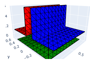
(a) Full multi-trace discretisation.

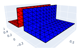
(b) Partial reduction.

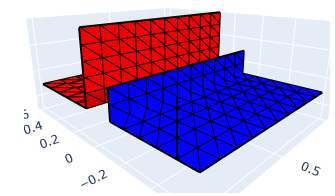
(c) Fixed overlap

(d) Single strip

Figure 5: Meshes illustrating full multi-trace discretization and three reduction strategies used here.

5 Numerical Results

5.1 Preconditioning the hypersingular operator (Neumann problem)

Consider the geometry in Figure 5. The structure is illuminated by a plane wave with signature $\exp\left(i\kappa x_{3}\right)$. The numerical experiments will be run in the low-frequency regime ($\kappa=1$) and the moderate frequency regime ($\kappa=10$).

Linear systems are solved using GMRES with the tolerance set to $2.0e-5$. To build the preconditioners, application of the inverse Gram matrix is required. This action is computed by running a second, inner GMRES solver within the outer, primal solver. Numerical experiments have shown that it is important to set the tolerance for this inner GMRES sufficiently low. In the experiments presented here the tolerance is set to $2.0e-12$. Fortunately the Gram matrices are well conditioned and application of their inverses through GMRES can be computed in a small and linear number of operations, even at these very small tolerances.

Another important aspect of implementing the preconditioning strategies presented above is the use of high quality quadrature rules, especially for interactions between geometric elements that are close together. Specifically, it is important that left and right nullspaces of the discrete bilinear forms are invariant upon introduction of the quadrature error. One can either choose to adopt highly accurate quadrature rules or to use rules that are symmetric with respect to back-front mirroring across the multi-screen. Here we have opted for the highly accurate and kernel independent Sauter-Schwab rules described in Chapter 5 of [26].

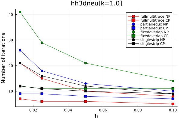
Figure 6: GMRES iterations vs $h$ at $\kappa=1$ for the Neumann problem at $\Gamma$ as in Figure 5.

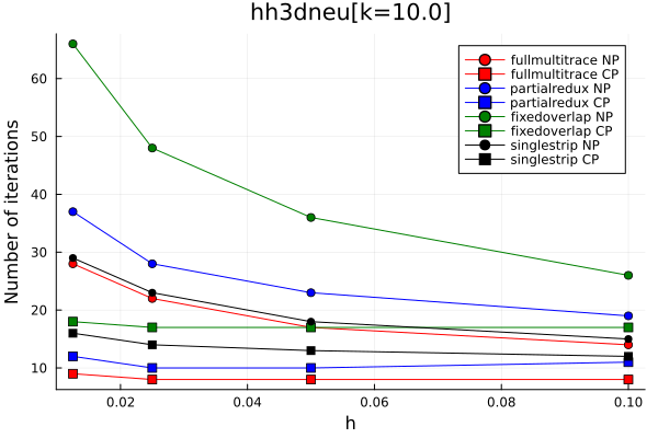
Figure 7: GMRES iterations vs $h$ at $\kappa=10$ for the Neumann problem at $\Gamma$ as in Figure 5.

The obtained results are displayed in Figure 6 for $\kappa=1$ and in Figure 7 for $\kappa=10$. There we label iteration counts for the unpreconditioned system by NP, and those for after Calderón preconditioning by CP. In both the low frequency and the moderate frequency case we find a much smaller number of iterations is required upon application of our operator preconditioning approach. For all four considered reductions of the $\mathbb{X}_{h}(\Gamma)$ depicted in Figure 5, there is a clear improvement. After preconditioning there remains a slow increase in the number of iterations, commensurate with the logarithmic grow in the (44).

At moderate frequencies, both the original system and the preconditioned system require more iterations, but the benefits of applying operator preconditioning remain.

5.2 Preconditioning the weakly singular operator (Dirichlet problem)

We consider the same geometry, excitation and GMRES tolerance used to study our preconditioner for the Neumann problem. An important difference is that DoFs for the Dirichlet problem are linked to triangles of the mesh, as opposed to vertices. The support of the primal basis functions spans only a single triangle. The reduction of the multi-trace space can be done up to the point where there is no overlap between the simple screens that support the reduced finite element spaces.

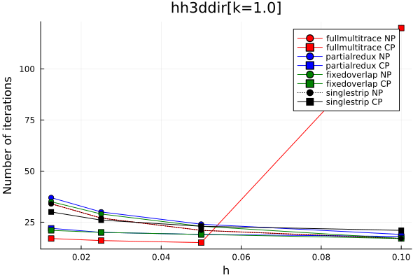
Figure 8: GMRES iterations vs $h$ at $\kappa=1$ for the Dirichlet problem at $\Gamma$ as in Figure 5.

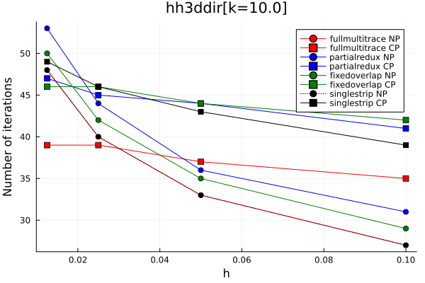
Figure 9: GMRES iterations vs $h$ at $\kappa=10$ for the Dirichlet problem at $\Gamma$ as in Figure 5.

Essentially all conclusions drawn for the Neumann problem carry over to the study of the numerical solution of the Dirichlet problem. In Figure 8 and Figure 9 it can be seen that at both frequencies and for all reduction strategies there is a clear decrease in the number of iterations required for solution. At moderate frequencies the performance of our preconditioner is less outspoken than for the Neumann problem. In fact, for the specific choice of the most aggressive reduction scheme the unpreconditioned system requires fewer iterations than the preconditioned system for all values of the mesh size $h$ we have investigated. Nevertheless, the trend in the corresponding lines in Figure 9 is such that a cross-over point is to be expected at only modestly smaller values for $h$.

5.3 Application to multi-screens of Type B

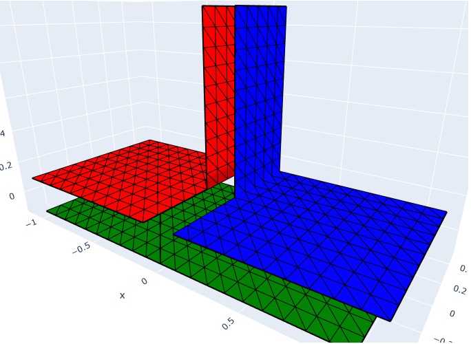
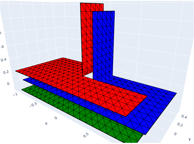
Figure 10: Two possible coverings for $[\Gamma]$. The most economic covering on the left precludes the definition of finite element spaces of direct product type (left). Allowing part of $[\Gamma]$ to be multiply covered resolves this problem (right).

For multi-screens of Type B, slight modifications to the choice of finite element spaces are required in order to arrive at a linear system requiring only few iterations for its solution. It may seem most natural to write $[\Gamma]$ as the union of the simple screens depicted on the left in Figure 10. Unfortunately, this partitioning does not allow the construction of a finite element space $\mathbb{X}_{h}(\Gamma)$ that can be written as the direct product of finite element spaces supported by the $\mathcal{I}_{i}$. The issue is that the solution for the Neumann problem in general will not be in $\prod_{i}\widetilde{H}^{1/2}(\mathcal{I}_{i})$ and that as a result degrees of freedom along the segment from $(0,0,0)$ to $(0,-0.5,0)$ cannot be discarded.

Allowing overlapping coverings of $[\Gamma]$ as depicted on the right of Figure 10 resolves this problem. For $l=1,..,m$, let $\bar{\mathcal{I}}_{l}$ denote either $\mathcal{I}_{l}$ with overlap when needed, or without overlap. We can use the finite element space $\prod_{i=1}^{m}\mathcal{S}^{1,0}(\bar{\mathcal{I}}_{i,h})$, which in a sense is larger than what we need but still leads to the correct quotient space.

We use this approach to solve the Neumann problem for the geometry in Figure 10 and for excitation $\exp(-i\kappa x_{3})$ with $\kappa=10$. Figure 11 demonstrates that upon preconditioning the number of iterations is much lower than what is required to solve the original linear system when solving the Neumann problem.

Figure 12 shows thee results for the Dirichlet problem. They are in line with those from Figigure 9: the higher offset in the iteration count results in a cross-over point at smaller values of $h$, but asymptotically the preconditioner leads to a more efficient algorithm.

The numerical results presented in this section have been produced with the boundary element package BEAST.jl. The scripts to reproduce them cam be found in a public Github repository.

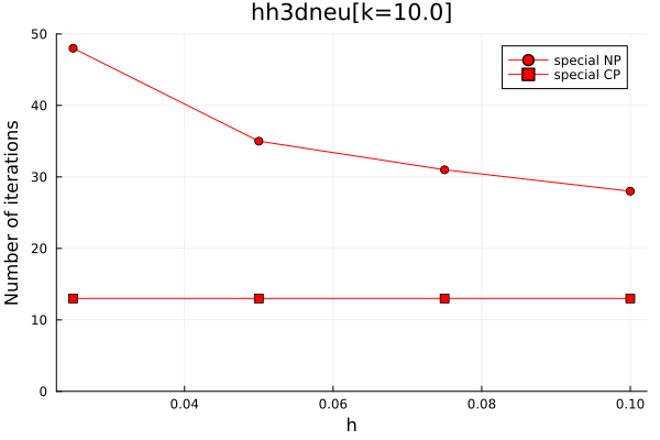
Figure 11: GMRES iterations vs $h$ at $\kappa=10$ for the Neumann problem for scattering by a geometry of type B.

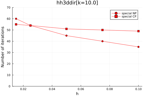
Figure 12: GMRES iterations vs $h$ at $\kappa=10$ for the Dirichlet problem for scattering by a geometry of type B.

6 Conclusions

We have presented an effective Calderón-type preconditioner for Helmholtz equations at multi-screens that builds on quotient-space BEM and operator preconditioning. Moreover, we have proved and confirmed numerically that it performs as standard Calderón preconditioning does on simple screens.

From a computational point of view, quotient-space BEM considering the full discretization of multi-valued traces has the advantage of requiring minimal geometrical information but the disadvantage of ”doubling DoFs”. As an alternative, we proposed different strategies to work with reduced multi-trace discretizations that use less DoFs but require more adaptations when using a standard BEM code. We gave details regarding the additional data requirements in the implementation of all these strategies, and used the developed framework to identify the requirements that reduced spaces need to meet in order to still have efficient Calderón-type preconditioning.

Finally, we briefly presented an heuristic strategy to precondition multi-screens that also appear in applications but that are not covered by our theory. Although in essence our approach follows the same principles of our Calderón-type preconditioner for type A multi-screens, rigorous analysis has been elusive and therefore has not been treated in this article. Indeed, the key missing piece is an extension of Lemma 8 for this case. Nevertheless, we offered numerical experiments to investigate its effectivity.

Current and future work also involves extending the analysis of this preconditioning approach to Maxwell equations, where numerical results are promising [14].

Funding

This project has received funding from the European Research Council (ERC) under the European Union’s Horizon 2020 research and innovation programme (Grant agreement No. 101001847) and from the Dutch Research Council (NWO) under the NWO-Talent Programme Veni with the project number VI.Veni.212.253.

Appendix A Auxiliary Lemmas

In this Section we prove some auxiliary results that hold for the multi-screens under consideration. We remark that for this we follow the cue from [8, Section 5.2] and use the properties of the associated volume-based spaces.

Let us begin by noticing that the Lipschitz partition $\left(\Omega_{j}\right)_{j=0\ldots n}$ such that $\Gamma\subset\cup_{j=0}^{m}\partial\Omega_{j}$ is not unique. We illustrate this for a two-dimensional triple junction $\Gamma$. in Fig. 13. Nevertheless, for the multi-screens considered in this paper, one can always find a Lipschitz partition such that $\Gamma\cap\partial\Omega_{i}\cap\partial\Omega_{j}\neq\emptyset$ for all $i,j=0,\dots,m$. In other words, we can always assume we have the configuration corresponding to Fig. 13(b). For simplicity of the proofs, this is the type of Lipschitz partitions that we will consider. This and the particular order of the domains is stated in the following:

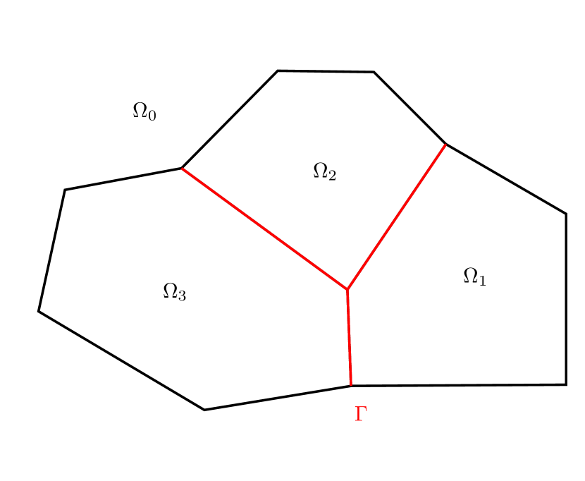
(a)

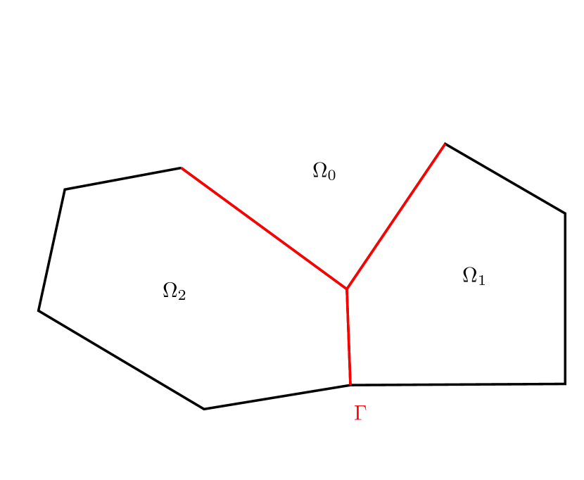
(b)

Figure 13: Example of two Lipschitz partitions for $\Gamma$ being a multi-screen with a triple junction.

Assumption 1.

Let $\left(\Omega_{j}\right)_{j=0\ldots n}$ be a Lipschitz partition in $\mathbb{R}^{3}$. We assume $\Gamma$ to be a multi-screen such that $\Gamma\subset\cup_{j=0}^{m}\partial\Omega_{j}$ and $\Gamma\cap\partial\Omega_{i}\cap\partial\Omega_{j}\neq\emptyset$ for all $i,j=0,\dots,m$. Moreover, and without loss of generality, we assume that $\Gamma$ and the Lipschitz partition $\left(\Omega_{j}\right)_{j=0\ldots n}$ are such that $\Omega_{0}$ is the exterior domain.

In order to improve readability of our auxiliary lemmas, let us define $S_{i}:=\Gamma\cap\partial\Omega_{i}$ for $i=0,\dots,m$. Now we are in the position to introduce the first result of this Appendix.

Lemma 2.

Let $\Gamma$ be a multi-screen as in Assumption 1. Then, the following injections hold

$$\mathbb{H}^{+\frac{1}{2}}(\Gamma)\xhookrightarrow{}H^{1/2}(S_{0})\times\dots\times H^{1/2}(S_{m}),$$

$$\mathbb{H}^{-\frac{1}{2}}(\Gamma)\xhookrightarrow{}H^{-1/2}(S_{0})\times\dots\times H^{-1/2}(S_{m}).$$

Proof.

We recall that $\mathbb{H}^{+\frac{1}{2}}(\Gamma)=H^{1}(\mathbb{R}^{d}\backslash\overline{\Gamma})/H^{1}_{0,\Gamma}(\mathbb{R}^{d})$ and note that $H^{1}(\mathbb{R}^{d}\backslash\overline{\Gamma})\subset H^{1}(\mathbb{R}^{d}\backslash\overline{\cup_{j=0}^{m}\partial\Omega_{j}})$. This induces the injection

$$\mathbb{H}^{+\frac{1}{2}}(\Gamma)=H^{1}(\mathbb{R}^{d}\backslash\overline{\Gamma})/H^{1}_{0,\Gamma}(\mathbb{R}^{d})\xhookrightarrow{}H^{1}(\mathbb{R}^{d}\backslash\overline{\cup_{j=0}^{m}\partial\Omega_{j}})/H^{1}_{0,\Gamma}(\mathbb{R}^{d}).$$

Additionally, we have the natural identification

$$H^{1}(\mathbb{R}^{d}\backslash\overline{\cup_{j=0}^{m}\partial\Omega_{j}})\cong H^{1}(\Omega_{0})\times\dots H^{1}(\Omega_{m}),$$

that associates $u\in H^{1}(\mathbb{R}^{d}\backslash\overline{\cup_{j=0}^{m}\partial\Omega_{j}})$ with $(u_{|\Omega_{0}},\dots,u_{|\Omega_{m}})$. From this natural identification, we get the isomorphism

$$H^{1}(\mathbb{R}^{d}\backslash\overline{\cup_{j=0}^{m}\partial\Omega_{j}})/H^{1}_{0,\Gamma}(\mathbb{R}^{d}) \cong[H^{1}(\Omega_{0})/H^{1}_{0,\Gamma}(\Omega_{0})]\times\dots\times[H^{1}(\Omega_{m})/H^{1}_{0,\Gamma}(\Omega_{m})]$$

$$\cong H^{1/2}(S_{0})\times\dots\times H^{1/2}(S_{m}).$$

Therefore, we have the injection

$$\mathbb{H}^{+\frac{1}{2}}(\Gamma)\xhookrightarrow{}H^{1/2}(S_{0})\times\dots\times H^{1/2}(S_{m}).$$

$\mathbb{H}^{-\frac{1}{2}}(\Gamma)\xhookrightarrow{}H^{-1/2}(S_{0})\times\dots\times H^{-1/2}(S_{m})$ follows analogously. ∎

Lemma 3.

Let $\Gamma$ be a multi-screen as in Assumption 1. Then, for $w\in\mathbb{H}^{+\frac{1}{2}}(\Gamma)$ and $\varphi\in\mathbb{H}^{-\frac{1}{2}}(\Gamma)$ such that $\varphi_{|S_{j}}\in\widetilde{H}^{-1/2}(S_{j})\,\forall\,j=0,\dots,m$, we have that

$$\ll w,\varphi\gg_{\Gamma}=\sum_{l=0}^{m}\langle w_{|S_{l}},\varphi_{|S_{l}}\rangle_{S_{l}}.$$ (46)

Proof.

Let us consider $w\in\mathbb{H}^{+\frac{1}{2}}(\Gamma)$ and $\varphi\in\mathbb{H}^{-\frac{1}{2}}(\Gamma)$. By definition

$$\ll w,\varphi\gg=\int\nolimits_{[\Gamma]}w\varphi\ d\sigma=\int_{\mathbb{R}^{d}\backslash\overline{\Gamma}}\mathbf{p}\cdot\nabla U+U\mathrm{div}(\mathbf{p})\ d\mathbf{x},$$

for $U\in H^{1}(\mathbb{R}^{d}\setminus\overline{\Gamma})$ and $\mathbf{p}\in\mathbf{H}(\mathrm{div},\mathbb{R}^{d}\setminus\overline{\Gamma})$ such that $\pi_{D}(U)=w$ and $\pi_{N}(\mathbf{p})=\varphi$.

For $j=0,\dots,m$, we set $U_{j}=U_{|\Omega_{j}}$ and $\mathbf{p}_{j}=\mathbf{p}_{|\Omega_{j}}$, and let $\mathbf{n}_{j}$ denote the outwards unit normal vector to $\Omega_{j}$. Then, by linearity of the integrals and Green’s formula, we get

$$\int_{\mathbb{R}^{d}\backslash\overline{\Gamma}}\mathbf{p}\cdot\nabla U+U\mathrm{div}(\mathbf{p})\ d\mathbf{x} =\sum_{j=0}^{m}\,\int_{\Omega_{j}}\mathbf{p}_{j}\cdot\nabla U_{j}+U_{j}\mathrm{div}(\mathbf{p}_{j})\ d\mathbf{x},$$

$$=\sum_{j=0}^{m}\,\int_{\partial\Omega_{j}}(U_{j})_{|\partial\Omega_{j}}\mathbf{n}_{j}\cdot(\mathbf{p}_{j})_{|\partial\Omega_{j}}d\sigma.$$ (47)

Now, let us point out that for any $j=0,\dots,m$ we know that functions in $H^{1}(\mathbb{R}^{d}\setminus\overline{\Gamma})$ and $\mathbf{p}\in\mathbf{H}(\mathrm{div},\mathbb{R}^{d}\setminus\overline{\Gamma})$ do not jump across $\partial\Omega_{j}\setminus\Gamma$. This allow us to simplify (47) further as

$$\sum_{j=0}^{m}\,\int_{\partial\Omega_{j}}(U_{j})_{|\partial\Omega_{j}}\mathbf{n}_{j}\cdot(\mathbf{p}_{j})_{|\partial\Omega_{j}}d\sigma=\int_{\Gamma}\sum_{j=0}^{m}v_{j}\mu_{j}d\sigma,$$ (48)

where $v_{j}=(U_{j})_{|\Gamma}$ and $\mu_{j}=\mathbf{n}_{j}\cdot(\mathbf{p}_{j})_{|\Gamma}$.

In order to see this, let us illustrate it for the case shown in Fig. 14. There $H^{1}(\mathbb{R}^{d}\setminus\overline{\Gamma})$ implies

$$U_{2}=U_{0}\>\text{ on }\partial\Omega_{2}\setminus\Gamma,\qquad\qquad U_{1}=U_{0}\>\text{ on }\partial\Omega_{1}\setminus\Gamma.$$ (49)

Similarly, since $\mathbf{p}\in\mathbf{H}(\mathrm{div},\mathbb{R}^{d}\setminus\overline{\Gamma})$ and $\mathbf{n}_{2}=-\mathbf{n}_{0}$ on $\partial\Omega_{2}\setminus\Gamma$, and $\mathbf{n}_{1}=\mathbf{n}_{0}$ on $\partial\Omega_{1}\setminus\Gamma$, we have

$$\mathbf{n}_{2}\cdot\mathbf{p}_{2}=-\mathbf{n}_{0}\cdot\mathbf{p}_{0}\>\text{ on }\partial\Omega_{2}\setminus\Gamma,\qquad\qquad\mathbf{n}_{1}\cdot\mathbf{p}_{1}=-\mathbf{n}_{0}\cdot\mathbf{p}_{0}\>\text{ on }\partial\Omega_{1}\setminus\Gamma.$$ (50)

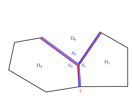
Figure 14: Example of a multi-screen $\Gamma$ with a triple junction. Here $\Gamma,S_{1},S_{2}$ and $S_{0}$ overlap, so they have been drawn slightly shifted for the sake of visibility.

Then

$$\sum_{j=0}^{2}\,\int_{\partial\Omega_{j}}(U_{j})_{|\partial\Omega_{j}}\mathbf{n}_{j}\cdot(\mathbf{p}_{j})_{|\partial\Omega_{j}}d\sigma=\sum_{j=0}^{2}\int_{\partial\Omega_{j}\setminus\Gamma}(U_{j})_{|\partial\Omega_{j}}\mathbf{n}_{j}\cdot(\mathbf{p}_{j})_{|\partial\Omega_{j}}d\sigma+\int_{\Gamma}\sum_{j=0}^{2}v_{j}\mu_{j}d\sigma.$$ (51)

Using (49) and (50) in (51), the terms on $\partial\Omega_{0}\setminus\Gamma$, $\partial\Omega_{1}\setminus\Gamma$ and $\partial\Omega_{2}\setminus\Gamma$ vanish, and we get

$$\sum_{j=0}^{2}\,\int_{\partial\Omega_{j}}(U_{j})_{|\partial\Omega_{j}}\mathbf{n}_{j}\cdot(\mathbf{p}_{j})_{|\partial\Omega_{j}}d\sigma=\int_{\Gamma}\sum_{j=0}^{2}v_{j}\mu_{j}d\sigma.$$

Next, let us continue with our proof and return to (48). We note that

$$\mu_{j}=\mathbf{n}_{j}\cdot(\mathbf{p}_{j})_{|\partial\Omega_{j}}=\pi_{N}(\mathbf{p}_{|\Omega_{j}})=(\pi_{N}(\mathbf{p}))_{|S_{j}}=\varphi_{|S_{j}}\in\widetilde{H}^{-1/2}(S_{j}),$$

$$v_{j}=(U_{j})_{|\partial\Omega_{j}}=\pi_{D}(U_{|\Omega_{j}})=(\pi_{D}(U))_{|S_{j}}=w_{|S_{j}}\in H^{1/2}(S_{j}).$$

This implies that on the right hand side of (48), we are allowed to split the integral over $\Gamma$ into the sum of the integrals over $S_{j}$ for $j=0,\dots,m$. Furthermore, we can write it in terms of the $H^{1/2}(S_{j})\times\widetilde{H}^{-1/2}(S_{j})$-duality pairings, i.e.

$$\int_{\Gamma}\sum_{j=0}^{m}v_{j}\mu_{j}d\sigma=\sum_{j=0}^{m}\int_{S_{j}}v_{j}\mu_{j}d\sigma=\sum_{j=0}^{m}\langle v_{j},\mu_{j}\rangle_{S_{j}}.$$

Finally, using again that $\mu_{j}=\varphi_{|S_{j}}$ and $v_{j}=w_{|S_{j}}$, we conclude that

$$\ll w,\varphi\gg_{\Gamma}=\sum_{j=0}^{m}\langle w_{|S_{j}},\varphi_{|S_{j}}\rangle_{S_{j}}.$$

∎

Analogously, one can prove:

Lemma 4.

Let $\Gamma$ be a multi-screen as in Assumption 1. Then, for $\varphi\in\mathbb{H}^{-\frac{1}{2}}(\Gamma)$ and $w\in\mathbb{H}^{+\frac{1}{2}}(\Gamma)$ such that $w_{|S_{j}}\in\widetilde{H}^{1/2}(S_{j})\,\forall\,j=0,\dots,m$, we have that

$$\ll w,\varphi\gg_{\Gamma}=\sum_{l=0}^{m}\langle w_{|S_{l}},\varphi_{|S_{l}}\rangle_{S_{l}}.$$ (52)

A.1 Inverse inequalities

In this section we will use a slightly different notation for our discrete multi-trace subspaces, just to allow them to be either in the primal or on the dual (virtual) mesh as introduced in Section 3. We consider

$$\mathbb{Z}_{h}^{1/2}(\Gamma)\subset\mathbb{H}^{+\frac{1}{2}}(\Gamma),\qquad\qquad\mathbb{Z}_{h}^{-1/2}(\Gamma)\subset\mathbb{H}^{-\frac{1}{2}}(\Gamma),$$

with $\dim(\mathbb{Z}_{h}^{1/2}(\Gamma))<\infty$ and $\dim(\mathbb{Z}_{h}^{-1/2}(\Gamma))<\infty$.

In order to present the main results of this Section, we need to introduce some existing results. Let us consider the simple screens $S_{j}$ for $j=0,\dots,m$ and the following finite dimensional spaces of piecewise polynomials:

$$\mathcal{S}^{0,-1}(S_{jh})\,:\,\text{ piecewise constants},\qquad\mathcal{S}^{1,0}(S_{jh})\,:\,\text{ piecewise linears}.$$

Lemma 5 ([19, Lemma 2.8]).

For $j=0,\dots,m$, the following inverse inequalities hold:

$$\|u_{h}\|_{\widetilde{H}^{1/2}(S_{j})} \leq c_{1}(1+|\log h|)\|u_{h}\|_{H^{1/2}(S_{j})},\qquad\forall u_{h}\in\mathcal{S}^{1,0}(S_{jh})\subset\widetilde{H}^{1/2}(S_{j}),$$ (53)

$$\|\varphi_{h}\|_{\widetilde{H}^{-1/2}(S_{j})} \leq c_{2}(1+|\log h|)\|\varphi_{h}\|_{H^{-1/2}(S_{j})},\qquad\forall\varphi_{h}\in\mathcal{S}^{0,-1}(S_{jh})\subset\widetilde{H}^{-1/2}(S_{j}),$$ (54)

for mesh size $h\leq 1$ and with constants $c_{1},c_{2}>0$ independent of $h$.

Next, we define two projection operators that will play a key role in their proofs. Let $\mathcal{S}^{1,0}(\check{S}_{jh})$ be the space of piecewise linears on the dual barycentric mesh of $S_{j}$, as defined in [3]. We introduce the generalized $L^{2}$-projection $\tilde{Q}_{h}^{j}:L^{2}(S_{j})\to\mathcal{S}^{1,0}(\check{S}_{jh})$ as

$$\langle\tilde{Q}_{h}^{j}u,\phi_{h}\rangle_{S_{j}}=\langle u,\phi_{h}\rangle_{S_{j}},\qquad\forall\phi_{h}\in\mathcal{S}^{0,-1}({S}_{jh}).$$ (55)

then, following [27, Theorems 2.1 and 2.2], one can show

Lemma 6 ([21, Theorem 4.3], Case A).

Let the family of meshes $\{S_{jh}\}_{h\in\mathcal{H}},h>0$ of a simple screen $S_{j}$ be uniformly shape-regular and locally quasi-uniform. Then, under certain (mild) local mesh conditions [27, Assumption 2.1], we have that

$$\|\tilde{Q}_{h}^{j}u\|_{H^{1/2}(S_{j})}\leq c_{Qj}\|u\|_{H^{1/2}(S_{j})},\qquad\forall u\in H^{1/2}(S_{j}),$$ (56)

and that the following inf-sup condition holds

$$\underset{v_{h}\in\mathcal{S}^{1,0}(\check{S}_{jh})}{\sup}\frac{|\langle\varphi_{h},v_{h}\rangle|}{\|v_{h}\|_{H^{1/2}(S_{j})}}\geq\frac{1}{c_{1}}\|\varphi_{h}\|_{\widetilde{H}^{-1/2}(S_{j})}\>,\qquad\forall\>\varphi_{h}\>\in\>\mathcal{S}^{0,-1}(S_{jh}),$$ (57)

with constants $c_{1}>0$ independent of $h$.

Remark 5.

The local mesh conditions [27, Assumption 2.1] are considered mild because they are fulfilled by a broad set of meshes used in applications, including geometrically graded meshes, algebraically 2-graded meshes and families of meshes generated by adaptive red-green algorithms [17].

Let us also introduce the projection operator $\Pi_{h}:\mathbb{H}^{+\frac{1}{2}}(\Gamma)\to\mathbb{Z}_{h}^{-1/2}(\Gamma)\subset\mathbb{H}^{-\frac{1}{2}}(\Gamma)$

$$\ll\Pi_{h}u,w_{h}\gg=(u,w_{h})_{\mathbb{H}^{+\frac{1}{2}}(\Gamma)}.$$ (58)

From [27, Thm. 2.1 and 2.2], we know that under certain (mild) local mesh conditions [27, Assumption 2.1] we satisfy the discrete inf-sup condition of the duality pairing of multi-trace spaces. Moreover, these mesh conditions also guarantee the continuity of $\Pi_{h}$, i.e.

$$\|\Pi_{h}u\|_{\mathbb{H}^{-\frac{1}{2}}(\Gamma)}\leq c_{\pi}\|u\|_{\mathbb{H}^{+\frac{1}{2}}(\Gamma)},\qquad\forall u\in\mathbb{H}^{+\frac{1}{2}}(\Gamma).$$ (59)

Therefore, in order to use the continuity of both projection operators, we will need to satisfy the following mesh assumption:

Assumption 2.

Let $\Gamma$ be a multi-screen as in Assumption 1.

We assume that for each $j=0,..,m$, the family of meshes $\{S_{jh}\}_{h\in\mathcal{H}},h>0$ of $S_{j}$ agree at the junction(s), are uniformly shape-regular, locally quasi-uniform and satisfy the (mild) local mesh conditions from [27, Assumption 2.1].

Lemma 7 (Inverse inequality in $\mathbb{H}^{-\frac{1}{2}}(\Gamma)$).

Let $\Gamma$ be a multi-screen as in Assumption 1 and $\mathbb{Z}_{h}^{1/2}(\Gamma)$ such that for all $v_{h}\in\mathbb{Z}_{h}^{1/2}(\Gamma)$ it holds that $(v_{h})_{|S_{j}}\in\widetilde{H}^{1/2}(S_{j})$. Then, we have that for all $\varphi_{h}\in\mathbb{Z}_{h}^{-1/2}(\Gamma)$

$$\|\varphi_{h}\|_{\mathbb{H}^{-\frac{1}{2}}(\Gamma)}\leq\widetilde{C}_{N}(1+|\log h|)\left(\sum_{j=0}^{m}\|\varphi_{h}\|_{H^{-1/2}(S_{j})}^{2}\right)^{1/2},$$ (60)

with mesh size $h\leq 1$, and $\widetilde{C}_{N}$¿0 independent of $h$.

Proof.

By definition of dual norm and Lemma 3, we get

$$\|\varphi_{h}\|_{\mathbb{H}^{-\frac{1}{2}}(\Gamma)} =\underset{v\in\mathbb{H}^{+\frac{1}{2}}(\Gamma)\setminus\{0\}}{\sup}\dfrac{|\ll v,\varphi_{h}\gg|}{\|v\|_{\mathbb{H}^{+\frac{1}{2}}(\Gamma)}}=\underset{v\in\mathbb{H}^{+\frac{1}{2}}(\Gamma)\setminus\{0\}}{\sup}\dfrac{|\sum_{j=0}^{m}\langle v_{j},\varphi_{hj}\rangle_{S_{j}}|}{\|v\|_{\mathbb{H}^{+\frac{1}{2}}(\Gamma)}},$$ (61)

where we have set $v_{j}=v_{|S_{j}}$ and $\varphi_{hj}=(\varphi_{h})_{|S_{j}}$. Then, let us consider the index set $\mathcal{J}$ of all the indices $0\leq k\leq m$ such that $v_{k}\neq 0$. Thus, we have that

$$\dfrac{|\sum_{j=0}^{m}\langle v_{j},\varphi_{hj}\rangle_{S_{j}}|}{\|v\|_{\mathbb{H}^{+\frac{1}{2}}(\Gamma)}}=\dfrac{|\sum_{j\in\mathcal{J}}\langle v_{j},\varphi_{hj}\rangle_{S_{j}}|}{\|v\|_{\mathbb{H}^{+\frac{1}{2}}(\Gamma)}}.$$ (62)

Next, we derive two inequalities that will help us proceed. First, using the embedding from Lemma 2 and then Young’s inequality $m$-times, we can obtain

$$\|v\|^{2}_{\mathbb{H}^{+\frac{1}{2}}(\Gamma)}\geq\sum_{j\in\mathcal{J}}\|v_{j}\|^{2}_{H^{1/2}(S_{j})}\geq\dfrac{1}{|\mathcal{J}|}\left(\sum_{j\in\mathcal{J}}\|v_{j}\|_{H^{1/2}(S_{j})}\right)^{2}$$ (63)

where $|\mathcal{J}|$ is the size of the index set $\mathcal{J}$. Second, we remark that for a sum $\sum_{i=1}^{m^{*}}a_{i}$ with all coefficients $a_{i}>0$ and $m^{*}\in\mathbb{N}$, we have that $\dfrac{1}{\sum_{i=1}^{m^{*}}a_{i}}\leq\dfrac{1}{a_{k}}$ for all $k=1,\dots m^{*}$. Hence,

$$\dfrac{m^{*}}{\sum_{i=1}^{m^{*}}a_{i}}\leq\sum_{k=1}^{m^{*}}\dfrac{1}{a_{k}}$$ (64)

Plugging these in (61) gives

$$\|\varphi_{h}\|_{\mathbb{H}^{-\frac{1}{2}}(\Gamma)} \overset{\eqref{eq:aux1}}{=}\underset{v\in\mathbb{H}^{+\frac{1}{2}}(\Gamma)\setminus\{0\}}{\sup}\dfrac{|\sum_{j\in\mathcal{J}}\langle v_{j},\varphi_{hj}\rangle_{S_{j}}|}{\|v\|_{\mathbb{H}^{+\frac{1}{2}}(\Gamma)}}\quad\quad\quad\overset{\eqref{eq:aux2}}{\leq}|\mathcal{J}|^{1/2}\underset{v\in\mathbb{H}^{+\frac{1}{2}}(\Gamma)\setminus\{0\}}{\sup}\dfrac{|\sum_{j\in\mathcal{J}}\langle v_{j},\varphi_{hj}\rangle_{S_{j}}|}{\sum_{k\in\mathcal{J}}\|v_{k}\|_{H^{1/2}(S_{k})}}$$

$$\overset{\eqref{eq:aux3}}{\leq}\dfrac{1}{|\mathcal{J}|^{1/2}}\underset{v\in\mathbb{H}^{+\frac{1}{2}}(\Gamma)\setminus\{0\}}{\sup}|\sum_{j\in\mathcal{J}}\dfrac{\langle v_{j},\varphi_{hj}\rangle_{S_{j}}}{\|v_{j}\|_{H^{1/2}(S_{j})}}|\leq\dfrac{1}{|\mathcal{J}|^{1/2}}\underset{v\in\mathbb{H}^{+\frac{1}{2}}(\Gamma)\setminus\{0\}}{\sup}\sum_{j\in\mathcal{J}}\dfrac{|\langle v_{j},\varphi_{hj}\rangle_{S_{j}}|}{\|v_{j}\|_{H^{1/2}(S_{j})}}$$

$$\leq\dfrac{1}{|\mathcal{J}|^{1/2}}\sum_{j\in\mathcal{J}}\>\underset{w_{j}\in H^{1/2}(S_{j})\setminus\{0\}}{\sup}\dfrac{|\langle w_{j},\varphi_{hj}\rangle_{S_{j}}|}{\|w_{j}\|_{H^{1/2}(S_{j})}}=\dfrac{1}{|\mathcal{J}|^{1/2}}\sum_{j=0}^{m}\>\underset{w_{j}\in H^{1/2}(S_{j})\setminus\{0\}}{\sup}\dfrac{|\langle w_{j},\varphi_{hj}\rangle_{S_{j}}|}{\|w_{j}\|_{H^{1/2}(S_{j})}}.$$ (65)

Then, using $\tilde{Q}_{h}^{j}$ from (55) and its continuity (56), we get

$$\|\varphi_{h}\|_{\mathbb{H}^{-\frac{1}{2}}(\Gamma)} \leq\dfrac{1}{|\mathcal{J}|^{1/2}}\sum_{j=0}^{m}\>\underset{w_{j}\in H^{1/2}(S_{j})\setminus\{0\}}{\sup}\dfrac{|\langle\tilde{Q}_{h}^{j}w_{j},\varphi_{hj}\rangle_{S_{j}}|}{\|w_{j}\|_{H^{1/2}(S_{j})}}\leq\dfrac{1}{|\mathcal{J}|^{1/2}}\sum_{j=0}^{m}\>c_{Qj}\underset{w_{j}\in H^{1/2}(S_{j})\setminus\{0\}}{\sup}\dfrac{|\langle\tilde{Q}_{h}^{j}w_{j},\varphi_{hj}\rangle_{S_{j}}|}{\|\tilde{Q}_{h}^{j}w_{j}\|_{H^{1/2}(S_{j})}}$$

$$\leq\dfrac{1}{|\mathcal{J}|^{1/2}}\sum_{j=0}^{m}\>c_{Qj}\underset{w_{hj}\in\mathcal{S}^{0,1}(S_{jh})\setminus\{0\}}{\sup}\dfrac{|\langle w_{hj},\varphi_{hj}\rangle_{S_{j}}|}{\|w_{hj}\|_{H^{1/2}(S_{j})}}.$$ (66)

Using Cauchy-Schwarz, we obtain

$$\|\varphi_{h}\|_{\mathbb{H}^{-\frac{1}{2}}(\Gamma)} \leq\dfrac{1}{|\mathcal{J}|^{1/2}}\sum_{j=0}^{m}\>c_{Qj}\underset{w_{hj}\in\mathcal{S}^{0,1}(S_{jh})\setminus\{0\}}{\sup}\dfrac{\|w_{hj}\|_{H^{1/2}(S_{j})}\|\varphi_{hj}\|_{\widetilde{H}^{-1/2}(S_{j})}}{\|w_{hj}\|_{H^{1/2}(S_{j})}}\leq\dfrac{1}{|\mathcal{J}|^{1/2}}\sum_{j=0}^{m}\>c_{Qj}\|\varphi_{hj}\|_{\widetilde{H}^{-1/2}(S_{j})}$$ (67)

Using the inverse inequality on simple screens (54), we can further bound this as

$$\|\varphi_{h}\|_{\mathbb{H}^{-\frac{1}{2}}(\Gamma)} \leq c_{N}(1+|\log h|)\sum_{j=0}^{m}\>\|\varphi_{hj}\|_{H^{-1/2}(S_{j})},$$ (68)

with $c_{N}:=\dfrac{c_{2}\max(c_{Qj})}{|\mathcal{J}|^{1/2}}$.

For convenience, we can work the estimate a bit further

$$\|\varphi_{h}\|_{\mathbb{H}^{-\frac{1}{2}}(\Gamma)}^{2} \leq c_{N}^{2}(1+|\log h|)^{2}\left(\sum_{j=0}^{m}\>\|\varphi_{hj}\|_{H^{-1/2}(S_{j})}\right)^{2}\>\overset{\eqref{eq:aux2}}{\leq}|\mathcal{J}|c_{N}^{2}(1+|\log h|)^{2}\sum_{j=0}^{m}\>\|\varphi_{hj}\|_{H^{-1/2}(S_{j})}^{2},$$ (69)

which gives (60) with $\tilde{C}_{N}=c_{2}\max(c_{Qj})$. ∎

Lemma 8 (Inverse inequality in $\mathbb{H}^{+\frac{1}{2}}(\Gamma)$).

Let $\Gamma$ be a multi-screen as in Assumption 1 and $\mathbb{Z}_{h}^{-1/2}(\Gamma)$ such that for all $\mu_{h}\in\mathbb{Z}_{h}^{-1/2}(\Gamma)$ it holds that $(\mu_{h})_{|S_{j}}\in\widetilde{H}^{-1/2}(S_{j})$. Then, we have that for all $u_{h}\in\mathbb{Z}_{h}^{1/2}(\Gamma)$

$$\|u_{h}\|_{\mathbb{H}^{+\frac{1}{2}}(\Gamma)}\leq\widetilde{C}_{D}(1+|\log h|)\left(\sum_{j=0}^{m}\|u_{h}\|_{H^{1/2}(S_{j})}^{2}\right)^{1/2},$$ (70)

with mesh size $h\leq 1$, and $\widetilde{C}_{D}$¿0 independent of $h$.

Proof.

By definition and continuity of $\Pi_{h}$ (c.f. (59)), we have that

$$\|u_{h}\|_{\mathbb{H}^{+\frac{1}{2}}(\Gamma)}=\dfrac{|(u_{h},u_{h})_{\mathbb{H}^{+\frac{1}{2}}(\Gamma)}|}{\|u_{h}\|_{\mathbb{H}^{+\frac{1}{2}}(\Gamma)}}=\dfrac{|\ll u_{h},\Pi_{h}u_{h}\gg|}{\|u_{h}\|_{\mathbb{H}^{+\frac{1}{2}}(\Gamma)}}\leq c_{\pi}\dfrac{|\ll u_{h},\Pi_{h}u_{h}\gg|}{\|\Pi_{h}u_{h}\|_{\mathbb{H}^{-\frac{1}{2}}(\Gamma)}}.$$ (71)

For convenience, set $\varphi_{h}=\Pi_{h}u_{h}\in\mathbb{Z}_{h}^{-1/2}(\Gamma)$, and $\varphi_{hj}=(\varphi_{h})_{|S_{j}}$. By assumption, we have that $\varphi_{hj}\in\widetilde{H}^{-1/2}(S_{j})$. and thus we can apply Lemma 3 and split the duality pairing.

In the following, we will proceed in analogy to what we did in the proof of Lemma 7. For this, let us introduce the index set $\mathcal{J}$ of all the indices $0\leq k\leq m$ such that $\varphi_{hj}\neq 0$. Moreover, similarly to (63), one can derive

$$\|\mu\|^{2}_{\mathbb{H}^{-\frac{1}{2}}(\Gamma)}\geq\sum_{j\in\mathcal{J}}\|\mu_{j}\|^{2}_{H^{-1/2}(S_{j})}\geq\dfrac{1}{|\mathcal{J}|}\left(\sum_{j\in\mathcal{J}}\|\mu_{j}\|_{H^{-1/2}(S_{j})}\right)^{2}.$$ (72)

With this, we can bound (71) further as follows

$$\|u_{h}\|_{\mathbb{H}^{+\frac{1}{2}}(\Gamma)} \leq c_{\pi}|\mathcal{J}|^{1/2}\dfrac{|\sum_{j\in\mathcal{J}}\langle u_{hj},\varphi_{hj}\rangle_{S_{j}}|}{\sum_{k\in\mathcal{J}}\|\varphi_{hk}\|_{H^{-1/2}(S_{k})}}\overset{\eqref{eq:aux3}}{\leq}\dfrac{c_{\pi}}{|\mathcal{J}|^{1/2}}\sum_{j\in\mathcal{J}}\dfrac{|\langle u_{hj},\varphi_{hj}\rangle_{S_{j}}|}{\|\varphi_{hj}\|_{H^{-1/2}(S_{j})}}$$

$$\leq\dfrac{c_{\pi}}{|\mathcal{J}|^{1/2}}\sum_{j\in\mathcal{J}}\dfrac{\|u_{hj}\|_{H^{1/2}(S_{j})}\|\varphi_{hj}\|_{\widetilde{H}^{-1/2}(S_{j})}}{\|\varphi_{hj}\|_{H^{-1/2}(S_{j})}}.$$ (73)

Now, we use the inverse inequality (54) on $S_{j}$ and get

$$\|u_{h}\|_{\mathbb{H}^{+\frac{1}{2}}(\Gamma)}\leq\dfrac{c_{\pi}}{|\mathcal{J}|^{1/2}}c_{2}(1+\log h)\sum_{j\in\mathcal{J}}\|u_{hj}\|_{H^{1/2}(S_{j})}\leq\dfrac{c_{\pi}}{|\mathcal{J}|^{1/2}}c_{2}(1+\log h)\sum_{j=0}^{m}\|u_{hj}\|_{H^{1/2}(S_{j})}.$$

Finally, just as in Lemma 7, we point out that from this one can derive

$$\|u_{h}\|_{\mathbb{H}^{+\frac{1}{2}}(\Gamma)} \leq\tilde{C}_{D}(1+\log h)\left(\sum_{j=0}^{m}\|u_{hj}\|_{H^{1/2}(S_{j})}^{2}\right)^{1/2}.$$ (74)

∎

A.2 Norm equivalences

Recall that

$$\|u\|_{\widetilde{H}^{+\frac{1}{2}}([\Gamma])}=\inf_{x\in H^{+\frac{1}{2}}([\Gamma])}\|u+x\|_{\mathbb{H}^{+\frac{1}{2}}(\Gamma)},$$

and that $\mathcal{S}^{1,0}(\mathcal{T}_{h})$ is the space spanned by piecewise linear “continuous” functions on (the virtual mesh) $\mathcal{T}_{h}$. We define the norm

$$\|u\|_{\widetilde{H}^{+\frac{1}{2}}([\Gamma]),D}:=\inf_{x_{h}\in H^{+\frac{1}{2}}([\Gamma])\cap\mathcal{S}^{1,0}(\mathcal{T}_{h})}\|u+x_{h}\|_{\mathbb{H}^{+\frac{1}{2}}(\Gamma)},$$ (75)

and study its relation with the continuous jump norm.

Lemma 9.

Assume that there exists an operator $\mathsf{R}_{h}^{+}\,:\,\mathbb{H}^{+\frac{1}{2}}(\Gamma)\to\mathcal{S}^{1,0}(\mathcal{T}_{h})$ such that

• $\mathsf{R}_{h}^{+}$ is a h-uniformly bounded projection,

• $\mathsf{R}_{h}^{+}(H^{+\frac{1}{2}}([\Gamma]))\subseteq H^{+\frac{1}{2}}([\Gamma])\cap\mathcal{S}^{1,0}(\mathcal{T}_{h}).$

Then $\|\cdot\|_{\widetilde{H}^{+\frac{1}{2}}([\Gamma])}$ and $\|\cdot\|_{\widetilde{H}^{+\frac{1}{2}}([\Gamma]),D}$ are equivalent norms

Proof.

By definition, we have

$$\|u\|_{\widetilde{H}^{+\frac{1}{2}}([\Gamma])}\leq\|u\|_{\widetilde{H}^{+\frac{1}{2}}([\Gamma]),D}$$ (76)

Choose $u_{h}=\mathsf{R}_{h}^{+}u$ where $u\in\widetilde{H}^{+\frac{1}{2}}([\Gamma])\subset\mathbb{H}^{+\frac{1}{2}}(\Gamma)$. Then we have that

$$\|u_{h}\|_{\widetilde{H}^{+\frac{1}{2}}([\Gamma]),D}=\inf_{x_{h}\in H^{+\frac{1}{2}}([\Gamma])\cap\mathcal{S}^{1,0}(\mathcal{T}_{h})}\|u_{h}+x_{h}\|_{\mathbb{H}^{+\frac{1}{2}}(\Gamma)}.$$

Note that, by surjectivity of $\mathsf{R}_{h}^{+}$ and property (ii), there exists an $x\in H^{+\frac{1}{2}}([\Gamma])$ such that $x_{h}=\mathsf{R}_{h}^{+}x$. This allows us to write

$$\|u_{h}\|_{\widetilde{H}^{+\frac{1}{2}}([\Gamma]),D}=\inf_{x_{h}\in H^{+\frac{1}{2}}([\Gamma])}\|\mathsf{R}_{h}^{+}(u+x)\|_{\mathbb{H}^{+\frac{1}{2}}(\Gamma)}.$$

Since $\mathsf{R}_{h}^{+}$ is continuous, we further get

$$\|u_{h}\|_{\widetilde{H}^{+\frac{1}{2}}([\Gamma]),D}\leq\|\mathsf{R}_{h}^{+}\|\inf_{x_{h}\in H^{+\frac{1}{2}}([\Gamma])}\|u+x\|_{\mathbb{H}^{+\frac{1}{2}}(\Gamma)}=\|\mathsf{R}_{h}^{+}\|\|u_{h}\|_{\widetilde{H}^{+\frac{1}{2}}([\Gamma])}$$ (77)

for all $v_{h}\in\widetilde{H}^{+\frac{1}{2}}([\Gamma])\cap\mathcal{S}^{1,0}(\mathcal{T}_{h})$.

From this, we conclude that the two norms are equivalent. Furthermore, the fact that $\mathsf{R}_{h}^{+}$ is $h$-uniformly bounded guarantees that the related constants are $h$-independent. ∎

Similarly, one shows that for the norm

$$\|\mu\|_{\widetilde{H}^{-\frac{1}{2}}([\Gamma]),D}:=\inf_{\xi_{h}\in H^{-\frac{1}{2}}([\Gamma])\cap\mathcal{S}^{0,-1}(\mathcal{T}_{h})}\|\mu+\xi_{h}\|_{\mathbb{H}^{-\frac{1}{2}}(\Gamma)},$$ (78)

we have

Lemma 10.

Assume that there exists an operator $\mathsf{R}_{h}^{-}\,:\,\mathbb{H}^{-\frac{1}{2}}(\Gamma)\to\mathcal{S}^{0,-1}(\mathcal{T}_{h})$ such that

• $\mathsf{R}_{h}^{-}$ is a h-uniformly bounded projection,

• $\mathsf{R}_{h}^{-}(H^{-\frac{1}{2}}([\Gamma]))\subseteq H^{-\frac{1}{2}}([\Gamma])\cap\mathcal{S}^{0,-1}(\mathcal{T}_{h}).$

Then, there exists $C_{N}>0$ independent of $h$ such that

$$\|\varphi_{h}\|_{\widetilde{H}^{-\frac{1}{2}}([\Gamma])}\leq\|\varphi_{h}\|_{\widetilde{H}^{-\frac{1}{2}}([\Gamma]),D}\leq c_{N}\|\varphi_{h}\|_{\widetilde{H}^{-\frac{1}{2}}([\Gamma])}$$ (79)

for all $\varphi_{h}\in\widetilde{H}^{-\frac{1}{2}}([\Gamma])\cap\mathcal{S}^{0,-1}(\mathcal{T}_{h})$.

A.3 Condition number estimates for quotient space discretisations

Following the policy of operator preconditioning, we need to bound the spectral condition number $\kappa_{sp}(\mathbf{M}^{-1}\mathbf{B}_{h}\mathbf{M}^{-T}\mathbf{A}_{h})$ for the pairs $(\mathbf{A}_{h},\mathbf{B}_{h})=(\mathbf{W}_{\kappa,h},\mathbf{B}^{\mathsf{W}}_{\kappa,h})$, and $(\mathbf{A}_{h},\mathbf{B}_{h})=(\mathbf{V}_{\kappa,h},\mathbf{B}^{\mathsf{V}}_{\kappa,h})$. In other words, we are assuming that we have that

• the Galerkin matrix $\mathbf{B}_{h}$ arises from a continuous sesquilinear form $\mathsf{b}$ that satisfies a discrete inf-sup condition on the whole space $\mathbb{Y}_{h}(\Gamma)$;

• the Galerkin matrix $\mathbf{M}_{h}$ arises from a continuous sesquilinear form $\mathsf{m}$ that satisfies a discrete inf-sup condition on the whole space $\mathbb{X}_{h}(\Gamma)$;

• the Galerkin matrix $\mathbf{A}_{h}$ has a non-trivial nullspace $N_{h}(\Gamma):=\ker\mathsf{A}_{h}$. Moreover, its corresponding sesquilinear form $\mathsf{a}$ satisfies a discrete inf-sup condition only on $\mathbb{X}_{h}(\Gamma)/N_{h}(\Gamma)$.

Since $\mathbf{A}_{h}$ is either $\mathbf{W}_{\kappa,h}$ or $\mathbf{V}_{\kappa,h}$, we will directly use that $N_{h}(\Gamma)=X_{h}(\Gamma)$ to avoid unnecessary extra notation.

As usual, this entails bounding $\lambda_{\max}:=\lambda_{\max}(\mathbf{M}^{-1}\mathbf{B}_{h}\mathbf{M}^{-T}\mathbf{A}_{h})$ from above and $\lambda_{\min}:=\lambda_{\min}(\mathbf{M}^{-1}\mathbf{B}_{h}\mathbf{M}^{-T}\mathbf{A}_{h})$ from below. In order to write these bounds, we need to introduce some notation first.

Let $\mathsf{A}_{h}\,:\,\mathbb{X}_{h}(\Gamma)\to\mathbb{X}_{h}(\Gamma)^{\prime}$, $\mathsf{B}_{h}\,:\,\mathbb{Y}_{h}(\Gamma)\to\mathbb{Y}_{h}(\Gamma)^{\prime}$ and $\mathsf{M}_{h}\,:\,\mathbb{X}_{h}(\Gamma)\to\mathbb{Y}_{h}(\Gamma)^{\prime}$ be the bounded linear operators associated to the sesquilinear forms $\mathsf{a}$, $\mathsf{b}$ and $\mathsf{m}$, respectively.

For $\lambda_{\max}$ we proceed in the classical way and arrive to

$$\lambda_{\max} \leq\|\mathsf{M}^{-1}\|^{2}\|\mathsf{B}\|\|\mathsf{A}$$

$$=\alpha_{\mathsf{M}}^{2}\|\mathsf{B}\|\|\mathsf{A}\|,$$ (80)

where

$$\small\alpha_{\mathsf{M}}:=\inf_{v_{h}\in\mathbb{X}_{h}(\Gamma)\setminus\{0\}}\dfrac{\|\mathsf{M}_{h}v_{h}\|_{\mathbb{Y}(\Gamma)^{\prime}}}{\|v_{h}\|_{\mathbb{X}(\Gamma)}}.$$

For $\lambda_{\min}$ we have to take a slightly different approach since we need to restrict $\mathsf{A}_{h}$ to the space where its corresponding bilinear form $\mathsf{a}$ satisfies a discrete inf-sup condition. Moreover, we need to establish when the discrete inf-sup condition will bound the smallest eigenvalue. We study this in the next Lemma.

Lemma 11 (Discrete inf-sup constant in the quotient space norm).

Let $\mathsf{a}$ be a continuous bilinear form on $\mathbb{X}(\Gamma)\times\mathbb{X}(\Gamma)$. Let $X(\Gamma)\subseteq\mathbb{X}(\Gamma)$ be both the left and right nullspace of $\mathsf{a}$.

Let $\mathbb{X}_{h}(\Gamma)$ be a finite dimensional subspace of $\mathbb{X}(\Gamma)$ and $\mathsf{A}_{h}\,:\,\mathbb{X}_{h}(\Gamma)\to\mathbb{X}_{h}(\Gamma)^{\prime}$ the bounded linear operator associated to $\mathsf{a}$. We assume that $\mathbb{X}_{h}(\Gamma)$ is nullspace conforming to $\mathsf{a}$ in the sense that $X_{h}(\Gamma):=\ker\mathsf{A}_{h}=\ker\mathsf{A}^{\prime}_{h}$ is a linear subspace of $X(\Gamma)\cap\mathbb{X}_{h}(\Gamma)\subseteq X(\Gamma)$.

If $\mathsf{a}$ satisfies a discrete inf-sup condition in the quotient space $\mathbb{X}_{h}(\Gamma)/X_{h}(\Gamma)\times\mathbb{X}_{h}(\Gamma)/X_{h}(\Gamma)$ with constant $\alpha_{\mathsf{a}}>0$ and if the norms on $\mathbb{X}(\Gamma)/X(\Gamma)$ and $\mathbb{X}(\Gamma)/X_{h}(\Gamma)$ are equivalent, then

$$\sup_{v_{h}\in\mathbb{X}_{h}(\Gamma)\setminus\{0\}}\frac{\mathsf{a}(u_{h},v_{h})}{\|v_{h}\|_{\mathbb{X}(\Gamma)}}\geq\tilde{\alpha}_{\mathsf{a}}\|u_{h}\|_{\mathbb{X}(\Gamma)/X(\Gamma)}.$$ (81)

Proof.

We note that due to the kernel, the supremum is not attained at $v_{h}\in X_{h}(\Gamma)$, and thus

$$\sup_{v_{h}\in\mathbb{X}_{h}(\Gamma)\setminus\{0\}}\frac{\mathsf{a}(u_{h},v_{h})}{\|v_{h}\|_{\mathbb{X}(\Gamma)}}\geq\sup_{\tilde{v}_{h}\in X_{h}(\Gamma)^{\perp}\setminus\{0\}}\frac{\mathsf{a}(u_{h},\tilde{v}_{h})}{\|\tilde{v}_{h}\|_{\mathbb{X}(\Gamma)}}$$ (82)

Let $\mathbb{Q}_{h}:\mathbb{X}_{h}(\Gamma)\to X_{h}(\Gamma)^{\perp}$ be an orthogonal projection with respect to the $\mathbb{X}(\Gamma)$-inner product. Using that $\tilde{v}_{h}=\mathbb{Q}_{h}\tilde{v}_{h}$, and the identification of $X_{h}(\Gamma)^{\perp}$ with $\mathbb{X}_{h}(\Gamma)/X_{h}(\Gamma)$, we have that by property of quotient spaces [5, Eq. (4)]

$$\sup_{\tilde{v}_{h}\in X_{h}(\Gamma)^{\perp}\setminus\{0\}}\frac{\mathsf{a}(u_{h},\tilde{v}_{h})}{\|\tilde{v}_{h}\|_{\mathbb{X}(\Gamma)}} =\sup_{\tilde{v}_{h}\in X_{h}(\Gamma)^{\perp}\setminus\{0\}}\frac{\mathsf{a}(u_{h},\tilde{v}_{h})}{\|\mathbb{Q}_{h}\tilde{v}_{h}\|_{\mathbb{X}(\Gamma)}}=\sup_{\tilde{v}_{h}\in\mathbb{X}_{h}(\Gamma)/X_{h}(\Gamma)\setminus\{0\}}\frac{\mathsf{a}(u_{h},\tilde{v}_{h})}{\|\tilde{v}_{h}\|_{\mathbb{X}(\Gamma)/X_{h}(\Gamma)}}.$$ (83)

Finally, by norm equivalence, this becomes the discrete inf-sup condition, i.e.

$$\sup_{v_{h}\in\mathbb{X}_{h}(\Gamma)\setminus\{0\}}\frac{\mathsf{a}(u_{h},v_{h})}{\|v_{h}\|_{\mathbb{X}(\Gamma)}} \geq c\,\sup_{\tilde{v}_{h}\in\mathbb{X}_{h}(\Gamma)/X_{h}(\Gamma)\setminus\{0\}}\frac{\mathsf{a}(u_{h},\tilde{v}_{h})}{\|\tilde{v}_{h}\|_{\mathbb{X}(\Gamma)/X(\Gamma)}}$$ (84)

$$\geq c\alpha_{\mathsf{a}}|u_{h}\|_{\mathbb{X}(\Gamma)/X(\Gamma)},$$ (85)

and therefore the required result follows with $\tilde{\alpha}_{\mathsf{a}}=c\alpha_{\mathsf{a}}$, where $c$ is the constant from the norm-equivalence. ∎

Using all the above, we can bound $\lambda_{\min}$ as follows

$$\lambda_{\min} =\inf_{u_{h}\in\mathbb{X}_{h}(\Gamma)/X_{h}(\Gamma)\setminus\{0\}}\dfrac{\|\mathsf{M}_{h}^{-1}\mathsf{B}_{h}\mathsf{M}^{-*}_{h}{\mathsf{A}_{h}}u_{h}\|_{\mathbb{X}(\Gamma)^{\prime}}}{\|u_{h}\|_{\mathbb{X}(\Gamma)}}\geq\alpha_{\mathsf{M}^{-1}}^{2}\alpha_{\mathsf{B}}\alpha_{\mathsf{a}},$$ (86)

with

$$\alpha_{\mathsf{M}^{-1}}:=\inf_{\mu_{h}\in\mathbb{Y}_{h}(\Gamma)^{\prime}\setminus\{0\}}\dfrac{\|\mathsf{M}_{h}^{-1}\mu_{h}\|_{\mathbb{X}(\Gamma)}}{\|\mu_{h}\|_{\mathbb{Y}(\Gamma)^{\prime}}}=\|\mathsf{M}\|^{-1},\qquad\qquad\alpha_{\mathsf{B}}:=\inf_{\xi_{h}\in\mathbb{Y}_{h}(\Gamma)\setminus\{0\}}\dfrac{\|\mathsf{B}_{h}\xi_{h}\|_{\mathbb{Y}(\Gamma)^{\prime}}}{\|\xi_{h}\|_{\mathbb{Y}(\Gamma)}}.$$

Finally, we combine (80) and (86) and get

$$\kappa_{sp}(\mathbf{M}^{-1}\mathbf{B}_{h}\mathbf{M}^{-T}\mathbf{A}_{h})\leq\dfrac{\alpha_{\mathsf{M}}^{2}\|\mathsf{B}\|\|\mathsf{A}\|}{\|\mathsf{M}\|^{2}\alpha_{\mathsf{B}}\tilde{\alpha}_{\mathsf{a}}}.$$ (87)

Remark 6.

Note that the nullspace conformity requirement forces us to use meshes that agree on the front and back of the structure. In practice this does not pose a major limitation because in a typical usage scenario the simple screens $\partial\Omega_{j}\cap\Gamma$ are built by fusing together two or more unique meshes for the interfaces $\partial\Omega_{i}\cup\partial\Omega_{j}$. The interface meshes are used both as front and back and thus necessarily agree.

Remark 7.

For the discrete quotient norm to be bounded from below by the continuous quotient norm, it suffices that $X_{h}(\Gamma)\subseteq X(\Gamma)\cap\mathbb{X}_{h}(\Gamma)$; equality is not required. This opens the door to reduction schemes for the multi-trace space variational formulation. A reduction scheme is a choice $\mathbb{X}_{h}(\Gamma)^{\circ}\subseteq\mathbb{X}_{h}(\Gamma)\subseteq\mathbb{X}(\Gamma)$ with corresponding discrete left/right nullspace $X_{h}(\Gamma)^{\circ}$ such that (i) $X_{h}(\Gamma)^{\circ}\subseteq X(\Gamma)$ and (ii) $\mathbb{X}_{h}(\Gamma)^{\circ}/X_{h}(\Gamma)^{\circ}=\mathbb{X}_{h}(\Gamma)/X_{h}(\Gamma)$. Such a choice leads on one hand to approximations in the jump space of equal quality and on the other hand does not preclude the construction of efficient operator preconditioners.

References

- [1] Martin Averseng. A stable and jump-aware projection onto a discrete multi-trace space, 2022. arXiv:2211.08223.
- [2] A. Buffa and S. H. Christiansen. The electric field integral equation on Lipschitz screens: definitions and numerical approximation. Numer. Math., 94(2):229–267, 2003.
- [3] A. Buffa and S. H. Christiansen. A dual finite element complex on the barycentric refinement. Mathematics of Computation, 76(260):1743–1769, 2007.
- [4] M. Carr, E. Topsakal, and J.L. Volakis. A procedure for modeling material junctions in 3-d surface integral equation approaches. IEEE Transactions on Antennas and Propagation, 52(5):1374–1378, 2004.
- [5] S. N. Chandler-Wilde, D. P. Hewett, and A. Moiola. Sobolev spaces on non-Lipschitz subsets of with application to boundary integral equations on fractal screens. Integral Equations Operator Theory, 87(2):179–224, 2017.
- [6] S. H. Christiansen and J.-C. Nédélec. Des préconditionneurs pour la résolution numérique des équations intégrales de frontière de l’acoustique. Comptes Rendus de l’Académie des Sciences - Series I - Mathematics, 330(7):617 – 622, 2000.
- [7] X. Claeys, L. Giacomel, R. Hiptmair, and C. Urzúa-Torres. Quotient-space boundary element methods for scattering at complex screens. BIT Numerical Mathematics, pages 1–29, 2021.
- [8] X. Claeys and R. Hiptmair. Integral equations on multi-screens. Integral Equations Operator Theory, 77(2):167–197, 2013.
- [9] X. Claeys and R. Hiptmair. Integral equations for electromagnetic scattering at multi-screens. Integral Equations Operator Theory, 84(1):33–68, 2016.
- [10] K. Cools and Francesco P. Andriulli. Well-conditioned saddle point description for scattering by a metallic junction. In 2015 International Conference on Electromagnetics in Advanced Applications (ICEAA), pages 1349–1352, 2015.
- [11] Kristof Cools. Mortar boundary elements for the efie applied to the analysis of scattering by pec junctions. In 2012 Asia-Pacific Symposium on Electromagnetic Compatibility, pages 165–168, 2012.
- [12] Kristof Cools and Francesco P. Andriulli. Accuracy of the calderon preconditioned efie for the scattering by pec junctions. In 2015 USNC-URSI Radio Science Meeting (Joint with AP-S Symposium), pages 144–144, 2015.
- [13] Kristof Cools and Francesco P. Andriulli. A regularised electric field integral equation for scattering by perfectly conducting junctions. In 2015 9th European Conference on Antennas and Propagation (EuCAP), pages 1–4, 2015.
- [14] Kristof Cools and Carolina Urzúa-Torres. Preconditioners for multi-screen scattering. In 2022 International Conference on Electromagnetics in Advanced Applications (ICEAA), pages 172–173, 2022.
- [15] V. J. Ervin and E. P. Stephan. A boundary element Galerkin method for a hypersingular integral equation on open surfaces. Math. Methods Appl. Sci., 13(4):281–289, 1990.
- [16] V. J. Ervin, E. P. Stephan, and S. Abou El-Seoud. An improved boundary element method for the charge density of a thin electrified plate in . Mathematical Methods in the Applied Sciences, 13(4):291–303, 1990.
- [17] Heiko Gimperlein, Jakub Stocek, and Carolina Urzúa-Torres. Optimal operator preconditioning for pseudodifferential boundary problems. Numer. Math., 148(1):1–41, 2021.
- [18] V. Girault and P.A. Raviart. Finite element methods for Navier–Stokes equations. Springer, Berlin, 1986.
- [19] N. Heuer. Preconditioners for the p-version of the boundary element Galerkin method in . habilitation, Uni Hannover, 1998.
- [20] R. Hiptmair. Operator preconditioning. Computers and Mathematics with Applications, 52(5):699–706, 2006.
- [21] R. Hiptmair, C. Jerez-Hanckes, and C. Urzúa-Torres. Optimal operator preconditioning for boundary elements on open curves. Technical Report 2013-48, Seminar for Applied Mathematics, ETH Zürich, Switzerland, 2013.
- [22] R. Hiptmair and C. Urzúa-Torres. Dual Mesh Operator Preconditioning On 3D Screens: Low-Order Boundary Element Discretization. Technical Report 2016-14, Seminar for Applied Mathematics, ETH Zürich, Switzerland, 2016.
- [23] Ralf Hiptmair, Carlos Jerez-Hanckes, and Carolina Urzúa-Torres. Optimal operator preconditioning for Galerkin boundary element methods on 3-dimensional screens. SIAM Journal on Numerical Analysis, 58(1):834–857, 2020.
- [24] W. McLean. Strongly Elliptic Systems and Boundary Integral Equations. Cambridge University Press, Cambridge, UK, 2000.
- [25] W. McLean and O. Steinbach. Boundary element preconditioners for a hypersingular integral equations on an interval. Adv. Comp. Math., 11(4):271–286, 1999.
- [26] Stefan A. Sauter and Christoph Schwab. Boundary element methods, volume 39 of Springer Series in Computational Mathematics. Springer-Verlag, Berlin, 2011. Translated and expanded from the 2004 German original.
- [27] O. Steinbach. Stability estimates for hybrid coupled domain decomposition methods, volume 1809 of Lecture Notes in Mathematics. Springer-Verlag, Berlin, 2003.
- [28] O. Steinbach and W.L. Wendland. The construction of some efficient preconditioners in the boundary element method. Adv. Comput. Math, 9:191–216, 1998.
- [29] Olaf Steinbach. Numerical approximation methods for elliptic boundary value problems. Springer, New York, 2008. Finite and boundary elements, Translated from the 2003 German original.
- [30] E.P. Stephan. Boundary integral equations for screen problems in . Integral Equations and Operator Theory, 10(2):236–257, 1987.
- [31] Pasi Yla-Oijala, Matti Taskinen, and Jukka Sarvas. Surface integral equation method for general composite metallic and dielectric structures with junctions. Progress In Electromagnetics Research, 52:81–108, 2005.