The special Two zeros texture based on $A_{4}$ symmetry and perturbation method

Abstract

The current study aimed to investigate the special case of two zeros in a Majorana neutrino mass matrix based on $A_{4}$ symmetry, where charged lepton mass matrix is diagonal. The texture $M_{\nu}^{S_{7}}$ with $(\mu,\mu)$ and $(\tau,\tau)$ vanishing element of mass matrix has magic and $\mu-\tau$ symmetry, with a tribimaximal form of the mixing matrix which leads to $\theta_{13}=0$ that it is not consistent with experimental data and does not seem to be allowed. Since $\theta_{13}$ is small compared to other neutrino mixing angles, we show that $\theta_{13}$, and $\delta$ could be obtained by using a complex symmetrical perturbation in the mass basis and also could be shown that $\delta m^{2}\equiv\leavevmode\nobreak\ m_{2}^{2}-m^{2}_{1}\neq 0$ affecting the atmospheric mixing angle.

We find that for the complex perturbation mass matrix, only the results of the case I, $\Delta<0$ and $\textit{Re}(\alpha)<0$, are consistent with experimental data. Furthermore, the allowed range of our parameter space and complex element of perturbation are found which led to finding the deviation of $\theta_{23}$ from $45^{\circ}$ where this deviation is in line with the experimental data which indicate the accuracy of our model and its results. Our prediction is inverted mass ordering in the Case I. The results of the case II, $\Delta>0$ and $\textit{Re}(\alpha)>0$, are ruled out.

I Introduction

In the last two decades, neutrino experiments have illustrated that neutrinos oscillate and are massive. Nevertheless, according to the standard parametrization, the unitary lepton mixing matrix, which connects the neutrino mass eigenstates to flavor eigenstates, is given by mixing1 ; mixing2 ; mixing3

$$U_{PMNS}=\left(\begin{array}[]{ccc}c_{12}c_{13}&s_{12}c_{13}&s_{13}e^{-i\delta}\\ -s_{12}c_{23}-c_{12}s_{23}s_{13}e^{i\delta}&c_{12}c_{23}-s_{12}s_{23}s_{13}e^{i\delta}&s_{23}c_{13}\\ s_{12}s_{23}-c_{12}c_{23}s_{13}e^{i\delta}&-c_{12}s_{23}-s_{12}c_{23}s_{13}e^{i\delta}&c_{23}c_{13}\end{array}\right),$$ (1)

where $c_{ij}\equiv\cos\theta_{ij}\text{ and }s_{ij}\equiv\sin\theta_{ij}$ (for $i,j=(1,2),(1,3)\text{ and }(2,3)$); $\delta$ is called the Dirac phase, analogous to the CKM phase.

Finally, consequences of the neutrino experiments such as T2K 26 ; 27 , RENO 28 , DOUBLE-CHOOZ 29 , and DAYA-BAY 30 ; 31 have indicated that there are a nonzero mixing angle $\theta_{13}$ which is small compared to the other two mixing ones and a possible nonzero Dirac CP-violation phase $\delta_{CP}$. Therefore, the Tribimaximal (TBM) mixing matrix is rejected 32 ; 33 . The TBM mixing matrix is TBM :

$$U_{TBM}=\left(\begin{array}[]{ccc}-\sqrt{\frac{2}{3}}&\frac{1}{\sqrt{3}}&0\\ \frac{1}{\sqrt{6}}&\frac{1}{\sqrt{3}}&-\frac{1}{\sqrt{2}}\\ \frac{1}{\sqrt{6}}&\frac{1}{\sqrt{3}}&\frac{1}{\sqrt{2}}\end{array}\right),$$ (2)

where, regardless of the model, the mixing angles are: $\theta_{12}\approx{35.26}^{\circ}$, $\theta_{13}\approx 0$, and $\theta_{23}\approx 45^{\circ}$ 25 .

Prior to this observation, models leading to the TBM mixing matrix, widely studied 256 ; 259 . Therefore, in order to produce $\theta_{13}\neq 0$ starting from an initial TBM mixing matrix, different approaches have been adopted 2591 . One of the successful phenomenological neutrino mass models with flavor symmetry, which is an appropriate framework for understanding the family structure of charged-lepton and of neutrino mass matrices ma ; ma1 , is illustrated by the group $A_{4}$ 16 ; 17 ; 18 ; 19 ; 20 ; 21 ; 22 ; 23 ; 24 . The $A_{4}$ is a symmetry group of the tetrahedron, was initially presented to illustrate a TBM mixing matrix 18 . Although, the primary initial objective of the $A_{4}$ models was illustrating a TBM mixing matrix 18 , many efforts, e.g., 16 ; 17 , 19 ; 20 ; 21 ; 22 ; 23 ; 24 , 38 , 39 , 43 ; 44 ; 45 ; 46 , have been made to set up a model capable of describing the non-TBM mixing matrix phenomenology.

The present $3\sigma$ global fits for the existing and known neutrino oscillation parametersexp :

$$\delta m^{2}[10^{-5}eV^{2}] = (6.94-8.14),$$

$$|\Delta m^{2}|[10^{-3}eV^{2}] = (2.47-2.63)-(2.37-2.53),$$

$$\sin^{2}\theta_{12} = (0.271-0.369),$$

$$\sin^{2}\theta_{23} = (0.434-0.610)-(0.433-0.608),$$

$$\sin^{2}\theta_{13} = (0.02000-0.02405)-(0.02018-0.02424),$$

$$\delta = (128^{\circ}-359^{\circ})-(200^{\circ}-353^{\circ}),$$ (3)

multiple sets of allowed ranges are stated, and the left and the right columns correspond to normal hierarchy and inverted hierarchy, respectively. $\delta m^{2}\equiv m_{2}^{2}-m_{1}^{2}$ and $\Delta m^{2}\equiv m_{3}^{2}-m_{1}^{2}$.

Despite the prevailing information about neutrino oscillation parameters (I), the mass and mixing problem in the lepton sector is still conceived as a fundamental problem.

In the current work, we mainly focused on the neutrinos based on especial case of two-zero textures with $A_{4}$ symmetry which is here called $M_{\nu}^{S_{7}}$ 200 . In 200 , we study all seven possible two-zero textures with $A_{4}$ symmetry, among which only two textures, the texture with $(e,e)$ and $(e,\mu)$ vanishing element of mass matrix and its permutation symmetry, are consistent with the experimental data in the non-perturbation method.

In this paper, we intend to consider $M_{\nu}^{S_{7}}$ in perturbation method to generate I) non-zero $\theta_{13}$, II) CP violation phase $\delta$ and III) deviations of $\theta_{23}$ from $\frac{\pi}{4}$. However, the discovery of the $\theta_{13}$, whose smallness (in comparison to other mixing angles) signifies modifying the neutrino mixing matrix by means of a small perturbation about the basic TBM mixing matrix. By employing different methods in a wide range of contexts, a lot of attempts have been made to generate some of the neutrino parameters in perturbation theory pur39 .

In the basis where the charged-lepton mass matrix is diagonal, a particular application of $A_{4}$ is given by ma1 :

$$\cal{M}_{\nu}=\left(\begin{array}[]{ccc}a+\frac{2d}{3}&b-\frac{d}{3}&c-\frac{d}{3}\\ b-\frac{d}{3}&c+\frac{2d}{3}&a-\frac{d}{3}\\ c-\frac{d}{3}&a-\frac{d}{3}&b+\frac{2d}{3}\end{array}\right),$$ (4)

which has also magic symmetry.

Various phenomenological textures, specifically texture zeros kumar ; z8 ; z9 ; z10 ; z11 ; z12 ; z13 ; z14 ; z15 ; permutation , have been investigated in both flavor and non-flavor bases. Such texture zeros not only causes to reduce the number of free parameters of neutrino mass matrix, but also contributes to establishing several simple and interesting relations between mixing angles. Therefore, in the current research, this allowed us to explore the effects of special case of two zero textures on $\cal{M}_{\nu}$ given by (4).

Moreover, assuming the Majorana nature of neutrinos, the present study strove to investigate the phenomenological implications of special case of two-zero textures of neutrino mass matrix together with $A_{4}$ symmetry, based on a global fit of current neutrino oscillation data exp . The special case of two-zero texture is $M_{\nu}^{S_{7}}$ with $(\mu,\mu)=0$, and $(\tau,\tau)=0$ which can expose the impressive phenomenological features of a defined Majorana neutrino mass matrix.

The organization of the paper is as follows. In Sec. II, the methodology is elaborated in two subsections. In subsection A, $M_{\nu}^{S_{7}}$ in the flavor bases was reconstructed as unperturbed Neutrino Mass Matrix, and also unperturbed neutrino mass matrix was obtained in the mass bases. In subsection B, the perturbed neutrino mass matrix was presented as a complex symmetric non-Hermitian matrix in the mass basis. The first-order of neutrino mass correction and the third mass eigenstate were obtained in the mass basis to first order corrections. Then $|\nu_{3}\rangle_{mass}$ in the flavor bases was rewritten and thereby $\sin^{2}{\theta_{13}}$, CP violation phase $\delta$ and $\tan^{2}{\theta_{23}}$ were obtained. In Sec. III, the results are compared with those of the experimental data in two different cases. In each case, the complex elements of perturbation, $\alpha$ and $\beta$, are illustrated onto the allowed region of the parameter space and their allowed region were found. In the case I, the allowed region of $\alpha$ and $\beta$ was acceptable; therefore, the magnitude of $\theta_{23}$ was obtained which was consistent with the experimental data and demonstrated the accuracy of our work. In the case II, the obtained region of $\alpha$ and $\beta$ was not acceptable; therefore it was ruled out. In Sec. IV, the conclusions are provided.

II Methodology

II.1 The Unperturbed Neutrino Mass Matrix

Assuming the Majorana nature of neutrinos, the mass matrix $\cal{M}_{\nu}$ is a complex symmetric matrix in Eq.  (4). We examine in (LABEL:200) the analysis of two-zero texture for the Majorana neutrino mass matrix based on $A_{4}$ symmetry, $\cal{M}_{\nu}$ in Eq. (4) restricts the number of probabally viable cases to seven. It is found that the texture with $(e,e)$ and $(e,\mu)$ vanishing elements of $\cal{M}_{\nu}$ in (4) and its permutation symmetry, are consistent with the experimental data in the non-perturbation method. The texture with $(e,\tau)=(\mu,\mu)=0$ and the texture with $(e,\mu)=(\mu,\mu)=0$ and their permutation symmetry, are not consistent with the experimental data at all in (LABEL:200). The seventh probably viable case of two-zero texture of $\cal{M}_{\nu}$ in Eq. (4) with $(\mu,\mu)=(\tau,\tau)=0$ is extremely interesting. We call it $M_{\nu}^{S_{7}}$ in (LABEL:200) and is given by;

$$\vspace{.2cm}M_{\nu}^{S_{7}}=\left(\begin{array}[]{ccc}a+\frac{2}{3}d&-d&-d\\ -d&0&a-\frac{d}{3}\\ -d&a-\frac{d}{3}&0\end{array}\right).$$ (5)

This mass matrix is a magic matrix, which obviously has $\mu-\tau$ symmetry. Consequently, it can lead to TBM mixing matrix  in Eq. (2) with $\theta_{13}=0$. Therefore, initially seems that $M_{\nu}^{S_{7}}$ in Eq. (5) is not allowed texture, but we consider it in perturbation method.

A straightforward diagonalization procedure yields $U_{TBM}^{T}M_{\nu}^{S_{7}}U_{TBM}=M_{diag}^{S_{7}}$, where

$$m_{1} = a+\frac{5}{3}d,$$

$$m_{2} = a-\frac{4}{3}d,$$

$$m_{3} = -a+\frac{1}{3}d,$$ (6)

the mass eigenvalues can be complex, they can be presented positive and real by phase transformation, as $diag=(1,e^{i\rho},e^{i\sigma})$, which $\rho$ and $\sigma$ are Majorana phases where neutrino oscillations are independent of them.

We reconstruct $M_{\nu}^{S_{7}}$ in Eq. (5) by using $M_{\nu}=U^{*}_{TBM}M_{diag}U^{\dagger}_{TBM}$, where $M_{\nu}$ is a magic neutrino mass matrix with $\mu-\tau$ symmetry. In this reconstruction, we define new parameters, as

$$m \equiv \frac{\sum m_{i}}{3}=\frac{(m_{1}+m_{2}+m_{3})}{3},$$

$$\Delta_{32} \equiv (m_{3}-m_{2}),$$

$$\Delta_{31} \equiv (m_{3}-m_{1}).$$ (7)

Also because of; the reported experimental results which have shown $\Delta m^{2}_{21}$ is tiny and greater than zero exp , we approximate $\Delta_{31}\simeq\Delta_{32}\equiv\Delta$. Therefore, the unperturbed mass matrix, the reconstructed $M_{\nu}^{S_{7}}$, in the flavor basis is;

$$M^{0}_{f\nu}\simeq\left(\begin{array}[]{ccc}m-\frac{\Delta}{3}&0&0\\ 0&m+\frac{\Delta}{6}&-\frac{\Delta}{2}\\ 0&-\frac{\Delta}{2}&m+\frac{\Delta}{6}\end{array}\right).$$ (8)

At this level, the unperturbed mass matrix $M^{0}_{f\nu}$ in Eq. (8) has $\mu-\tau$ symmetry but is no longer magic. The mass spectrum of $M^{(0)}_{f\nu}$ is

$$\vspace{.2cm}m^{(0)}_{1}=m^{(0)}_{2}=m-\frac{\Delta}{3},\leavevmode\nobreak\ \leavevmode\nobreak\ \leavevmode\nobreak\ \leavevmode\nobreak\ \text{and}\leavevmode\nobreak\ \leavevmode\nobreak\ \leavevmode\nobreak\ m^{(0)}_{3}=m+\frac{2\Delta}{3}.$$ (9)

Here $m^{(0)}_{1}$, $m^{(0)}_{2}$ and $m^{(0)}_{3}$ are real and positive and $m^{(0)}_{1}$, and $m^{(0)}_{2}$ are the same. Hence, the unperturbed mass matrix in the mass basis is;

$$M^{0}_{mass}\simeq\left(\begin{array}[]{ccc}m-\frac{\Delta}{3}&0&0\\ 0&m-\frac{\Delta}{3}&0\\ 0&0&m+\frac{2\Delta}{3}\end{array}\right).$$ (10)

In the mass basis the eigenstates of the unperturbed neutrino mass matrix $M^{0}_{mass}$ in Eq. (10)are as follows:

$$\vspace{.2cm}|\nu^{(0)}_{1}\rangle=\left(\begin{array}[]{ccc}1\\ 0\\ 0\end{array}\right),\leavevmode\nobreak\ \leavevmode\nobreak\ \leavevmode\nobreak\ \leavevmode\nobreak\ |\nu^{(0)}_{2}\rangle=\left(\begin{array}[]{ccc}0\\ 1\\ 0\end{array}\right),\leavevmode\nobreak\ \leavevmode\nobreak\ \leavevmode\nobreak\ \leavevmode\nobreak\ \leavevmode\nobreak\ |\nu^{(0)}_{3}\rangle=\left(\begin{array}[]{ccc}0\\ 0\\ 1\end{array}\right),$$ (11)

in which the first two mass eigenstates are degenerate and the columns of $U_{TBM}$ in Eq. (2) are the unperturbed flavour eigenstates.

We should mention that, up to now, the shortcomings are: (i) the absence of $m^{(0)}_{1}$, and $m^{(0)}_{2}$ splitting, (ii) the ordering of neutrino masses which is unknown and (iii) the mixing matrix which is still $U_{TBM}$. Thus, the main objective is obtaining the splitting of $m^{(0)}_{1}$, and $m^{(0)}_{2}$ by means of a mass perturbation, from which $\theta_{13}\neq 0$ and CP violation are also derived. Moreover, CP violation conditions are necessarily mandate in that $\mu-\tau$ symmetry should be broken. An interesting question is: After breaking the $\mu-\tau$ symmetry, will $\theta_{23}=45^{\circ}$ remain valid or not?

II.2 The perturbed Neutrino Mass Matrix and Perturbation

In our work, the minimal symmetric perturbation neutrino mass matrix in the mass basis can be written as ;

$$M^{\prime}_{mass}\simeq\Delta\left(\begin{array}[]{ccc}0&0&\beta\\ 0&\alpha&0\\ \beta&0&0\end{array}\right).$$ (12)

The dimensionless perturbation elements i.e., $\alpha,\beta$ can be real or complex and should be small compared to the elements of unperturbed neutrino mass matrix $M^{0}_{mass}$ in Eq. (10) for a valid perturbation theory.

If $M^{\prime}_{mass}$ is a complex symmetric non-Hermitian matrix given in Eq. (12), therefore we have to consider $(M^{0}_{mass}+M^{\prime}_{mass})^{\dagger}(M^{0}_{mass}+M^{\prime}_{mass})$ where we drop a term, which is ${\cal O}(\alpha^{2},\leavevmode\nobreak\ \beta^{2})$. ${M^{0}_{mass}}^{\dagger}M^{0}_{mass}$ is the unperturbed Hermitian term , and its eigenstates are the same as those of $M^{0}_{mass}$ in Eq. (11) and its eigenvalues are $(m^{(0)}_{1})^{2}$, $(m^{(0)}_{2})^{2}$ and $(m^{(0)}_{3})^{2}$, therefore the perturbation term is $M^{p}_{mass}={M^{0^{\dagger}}_{mass}}M^{\prime}_{mass}+{M^{\prime^{\dagger}}_{mass}}M^{0}_{mass}$ and the perturbation matrix is

$$M^{p}_{mass}\simeq\Delta\leavevmode\nobreak\ \left(\begin{array}[]{ccc}0&0&\textit{Re}(\beta)(2m+\frac{\Delta}{3})+\textit{Im}(\beta)(-\Delta)\\ 0&\textit{Re}(\alpha)(2m-\frac{2\Delta}{3})&0\\ \textit{Re}(\beta)(2m+\frac{\Delta}{3})+\textit{Im}(\beta)(\Delta)&0&0\end{array}\right).$$ (13)

The first-order corrections to the neutrino masses, in the mass basis Eq. (11), are obtained from $m_{i}^{(1)}\delta_{ij}=\langle\nu_{i}^{(0)}|{M^{0^{\dagger}}_{mass}}M^{\prime}_{mass}+{M^{\prime^{\dagger}}_{mass}}M^{0}_{mass}|\nu_{j}^{(0)}\rangle$. Therefore, by using Eq. (9) and the first-order of neutrino mass correction, we have

$$m_{1}^{2} = (m^{(0)}_{1})^{2},$$

$$m_{2}^{2} = (m^{(0)}_{2})^{2}+\textit{Re}(\alpha)(2m-\frac{2}{3}\Delta)\Delta,$$

$$m_{3}^{2} = (m^{(0)}_{3})^{2}.$$ (14)

The mass correction arises from this order corrections with $m_{2}^{(1)}\neq 0$, and $m_{1}^{(1)}=m_{3}^{(1)}=0$. Therefore, the splitting of $m_{1}$, and $m_{2}$ is equal to $m_{2}^{(1)}$. Neutrino experimental data have so far definitely confirmed that $\delta m^{2}=m_{2}^{2}-m_{1}^{2}>0$. Therefore, by using  Eq. (9) $m_{2}^{(1)}=\textit{Re}\alpha(2\leavevmode\nobreak\ m^{(0)}_{2})\Delta$ must be positive.

From equations in  Eq. (II.2), we could obtain the ratio of two neutrino mass-squared differences $R_{\nu}=\frac{\delta m^{2}}{\Delta m^{2}}$, as

$$\vspace{.2cm}R_{\nu}=\textit{Re}(\alpha)\frac{6m-2\Delta}{6m+\Delta},$$ (15)

where $\delta m^{2}\equiv m_{2}^{2}-m_{1}^{2}$ and $\Delta m^{2}\equiv m_{3}^{2}-m_{1}^{2}$.

We reproduce the third mass eigenstate $|\nu_{3}>$, in the mass basis to the first order corrections, by

$$|\nu_{3}>_{mass}=|\nu^{(0)}_{3}\rangle+\frac{<\nu^{(0)}_{j}|M^{p}_{mass}|\nu^{(0)}_{3}>}{(m^{(0)}_{3})^{2}-(m^{(0)}_{j})^{2}}|\nu^{(0)}_{j}\rangle,\;\;(j\neq 3).\;$$ (16)

Using Eq. (9), Eq. (11) and Eq. (13), we could obtain $|\nu_{3}>_{mass}$ as

$$|\nu_{3}>_{mass}=\left(\begin{array}[]{ccc}\textit{Re}(\beta)-\frac{3\Delta}{6m+\Delta}\textit{Im}(\beta)\\ 0\\ 1\end{array}\right).$$ (17)

Now, we rewrite $|\nu_{3}>_{mass}$ in  Eq. (17), in the flavor basis, as follows

$$|\nu_{3}>_{flavor}=\left(\begin{array}[]{ccc}\sqrt{\frac{2}{3}}\left(\frac{-3\Delta\textit{Im}(\beta)}{6m+\Delta}+\textit{Re}(\beta)\right)\\ \frac{1}{\sqrt{2}}-\frac{\frac{-3\Delta\textit{Im}(\beta)}{6m+\Delta}+\textit{Re}(\beta)}{\sqrt{6}}\\ -\frac{1}{\sqrt{2}}-\frac{\frac{-3\Delta\textit{Im}(\beta)}{6m+\Delta}+\textit{Re}(\beta)}{\sqrt{6}}\end{array}\right),$$ (18)

and then could obtain nonzero values for both $\sin\theta_{13}$ , $\delta$, and the deviation of $\theta_{23}$ from $45^{\circ}$ by comparing $|\nu_{3}>_{flavor}$ in  Eq. (18) with the third column of lepton mixing matrix  in  Eq. (1). Therefore,

$$\sin^{2}\theta_{13} = |U_{13}|^{2}=\frac{2}{3}(\textit{Re}(\beta))^{2}+\frac{6\Delta^{2}}{(6m+\Delta)^{2}}(\textit{Im}(\beta))^{2},$$

$$\tan\delta = \frac{(-3\Delta)\textit{Im}(\beta)}{(6m+\Delta)\textit{Re}(\beta)},$$

$$\tan\theta^{2}_{23} = \frac{|U_{23}|^{2}}{|U_{33}|^{2}}=1-\frac{4\sqrt{3}\textit{Re}(\beta)}{3+(\frac{3\Delta\textit{Im}(\beta)}{6m+\Delta})^{2}+2\sqrt{3}\textit{Re}(\beta)+(\textit{Re}(\beta))^{2}}.$$ (19)

Up to this point, having used perturbation method, we could obtain I)the splitting of the two first neutrino masses, II)the third perturbed mass eigenstate, in the mass basis Eq. (17) and also the flavor basis Eq. (18), in the CP violation case, therefor generating III)$\theta_{13}\neq 0$, VI)$\delta$, and V) the rate of $\theta_{23}$ deviation from $45^{\circ}$. In the next section, by comparing the results of our work those of the experimental data Eq. (I), we will show that $M_{\nu}^{S_{7}}$ (5) could be allowed texture.

III COMPARISON WITH EXPERIMENTAL DATA

In this section the results of the current study are compared with those of the experimental data. As it was mentioned in the previous section, according to neutrino experimental data, we have $\delta m^{2}=\textit{Re}(\alpha)(2\leavevmode\nobreak\ m^{(0)}_{2})\Delta>0$. Therefore, since $m^{(0)}_{2}$ in Eq. (9) is real and positive, we have two cases; I)$\Delta$ and $\textit{Re}(\alpha)$ to be negative, II)$\Delta$ and $\textit{Re}(\alpha)$ to be positive.

Initially, we consider the case I, when $\Delta<0$ and $\textit{Re}(\alpha)<0$. The investigation of the case I includes three steps, in the first step, we obtain the allowed range of $\textit{Re}(\alpha)$, as it is shown in Figure 1. We do this by substituting the experimental range of $R_{\nu}$  in Eq. (15) and mapping $\textit{Re}(\alpha)$ onto our parameter space of the case I, $-\frac{1}{3}\leq\frac{m}{\Delta}\leq 0$  , according to the experimental data of $R_{\nu}$.

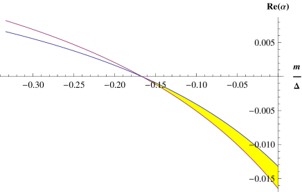
Figure 1: (color online). The range of $\textit{Re}(\alpha)$ onto $\frac{m}{\Delta}$ our parameter space, according to the experimental data of $R_{\nu}$. The yellow (dark) area displays the allowed region of $\textit{Re}(\alpha)$ within our model in the case I.

As regards the case I, $\Delta$ and $\textit{Re}(\alpha)$ must be negative; therefore, as it is shown in Figure 1 the allowed range of $\textit{Re}(\alpha)$ is restricted to the below of the horizontal axis, $(\frac{m}{\Delta})$ in the dark area between two curves. Therefore, the allowed range of $\textit{Re}(\alpha)$ is

$$\textit{Re}(\alpha)\approx\leavevmode\nobreak\ 0\rightarrow\leavevmode\nobreak\ -(0.0131-0.0161).$$ (20)

Likewise, as it is shown in Figure 1, we could to specify the allowed range of our parameter space, $\frac{m}{\Delta}$ according to the allowed range of $\textit{Re}(\alpha)$ as follows,

$$\frac{m}{\Delta}\approx\leavevmode\nobreak\ (-0.167-0).$$ (21)

In the second step , we obtain the allowed range of $\frac{\textit{Im}(\beta)}{\textit{Re}(\beta)}$. As it is shown in Figure 2, we do this by using the equation of $\tan\delta$ in Eq. (II.2) and mapping $\frac{\textit{Im}(\beta)}{\textit{Re}(\beta)}$ onto the allowed range of our parameter space  Eq. (21) according to the experimental data of $\tan\delta$  in Eq. (I).

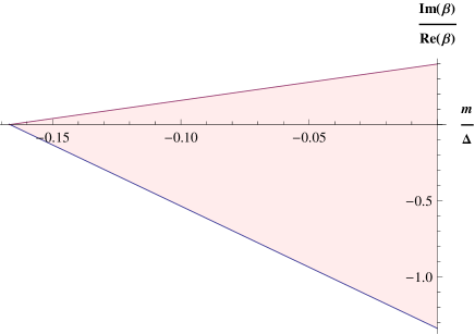
Figure 2: (color online). The dark area is the allowed range of $\frac{\textit{Im}(\beta)}{\textit{Re}(\beta)}$ onto $\frac{m}{\Delta}$ our parameter space, according to the experimental data of $\tan\delta$.

Therefore, we obtain the allowed region of $\frac{\textit{Im}(\beta)}{\textit{Re}(\beta)}$ onto our parameter space which is consistent with the experimental data as follows

$$\frac{\textit{Im}(\beta)}{\textit{Re}(\beta)}\approx((-1.31)-0.4),$$ (22)

accordingly, can write

$$\textit{Im}(\beta)\approx((-1.31)-0.4){\textit{Re}(\beta)},$$ (23)

therefore, in the second step, we obtain the ratio of $\frac{\textit{Im}(\beta)}{\textit{Re}(\beta)}$.

In the third step, we obtain the allowed range of $\textit{Re}(\beta)$, as it is shown in Figure 3, and subsequently the allowed range of ${\textit{Im}(\beta)}$ by using Eq. (23). We do this by using the equation of $\sin^{2}\theta_{13}$ in Eq. (II.2) and mapping $\textit{Re}(\beta)$ onto our parameter space Eq. (21), according to the experimental data of $\sin^{2}\theta_{13}$ in Eq. (I).

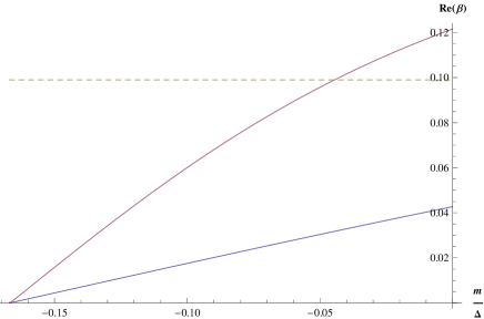
Figure 3: (color online). Range of $\textit{Re}(\beta)$ onto $\frac{m}{\Delta}$ our parameter space, according to the experimental data of $\sin^{2}\theta_{13}$. The area bellow the line $0.099$ displays the allowed region of $\textit{Re}(\beta)$ within our model.

According to perturbation theory, the perturbation elements i.e., $\alpha$, and $\beta$ in Eq. (12) should be small compared to the elements of unperturbed neutrino mass matrix $m$, and $\Delta$  in Eq. (10). Accordingly, we only accept those values of $\textit{Re}(\beta)$ that are less than $0.1$. Therefore, the area bellow the line $0.099$ in figure 3 displays the allowed region of $\textit{Re}(\beta)$ within our model, as

$$\textit{Re}(\beta)\approx\leavevmode\nobreak\ 0\rightarrow(0.043-0.099),$$ (24)

then based on Eq. (23), and Eq. (23) the allowed region of $\textit{Im}(\beta)$ is

$$\textit{Im}(\beta)\approx\leavevmode\nobreak\ 0\rightarrow((-0.056)-0.04),$$ (25)

Having taken these three steps, we obtain the allowed region of our parameter space,$\frac{m}{\Delta}$ in Eq. (21), and dimensionless perturbation elements $\textit{Re}(\alpha)$, $\textit{Re}(\beta)$, and $\textit{Im}(\beta)$ (25), respectively in Eq. (20), Eq. (24), and Eq. (25).

Now we must examine the accuracy of the results of the case I by determining the magnitude of $\tan\theta^{2}_{23}$ in Eq. (II.2) by values of our parameter obtained in the pervious three steps. We plot $\tan\theta^{2}_{23}$, based on the allowed region of perturbation elements, onto parameter space as it is shown in Figure 4. Interestingly, the values obtained for $\tan\theta^{2}_{23}$ corroborate those of with the experimental data  in Eq. (I). We find the allowed region of $\theta_{23}$ in the case I as

$$\theta_{23}\approx(41.81^{\circ}-43.96^{\circ})\rightarrow\leavevmode\nobreak\ 45^{\circ},$$ (26)

which indicate the accuracy of the case I in our work .

Figure 4: (color online). Range of $\tan\theta^{2}_{23}$ onto $\frac{m}{\Delta}$ parameter space, according to the allowed range of perturbation elements. The dark area displays the allowed region of $\tan\theta^{2}_{23}$ within our model which in complete agreement with the experimental data  in Eq. (I).

Also according to the sign of $\Delta$ and $\textit{Re}(\beta)$ in this case, the neutrino mass ordering is inverted.

Now we consider the case II when $\Delta$ and $\textit{Re}(\alpha)$ are both positive. In this case, similar to the case I, we first obtain the allowed range of $\textit{Re}(\alpha)$, as it is shown in Figure 5. We do this by substituting the experimental range of $R_{\nu}$  in Eq. (15) and mapping $\textit{Re}(\alpha)$ onto our parameter space of the case II, $\frac{m}{\Delta}\geq\frac{1}{3}$ /footnoteThe allowed range of our parameter space based on $m^{(0)}_{2}>0$, according to the experimental data in Eq. (I).

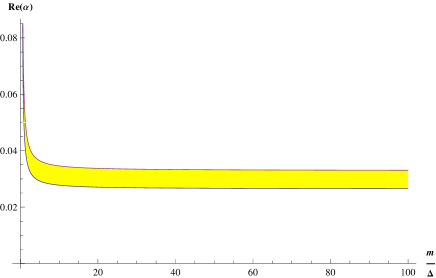
Figure 5: (color online). The range of $\textit{Re}(\alpha)$ onto $\frac{m}{\Delta}$, our parameter space of the case II, according to the experimental data of $R_{\nu}$. The allowed range of $\textit{Re}(\alpha)$ is restricted in the dark region between two parallel horizontal lines in the case II.

Therefore in Case II, according to Figure 5, the allowed range of $\textit{Re}(\alpha)$ which is restricted in the dark region is

$$\textit{Re}(\alpha)\approx\leavevmode\nobreak\ (0.0281-0.04)\rightarrow\infty.$$ (27)

In the next step, we find the allowed range of $\frac{\textit{Im}(\beta)}{\textit{Re}(\beta)}$ in the case II as shown in Figure 6. Same as the case I, we do this by using the equation of $\tan\delta$ in Eq. (II.2) and mapping $\frac{\textit{Im}(\beta)}{\textit{Re}(\beta)}$, but onto the allowed range of our parameter space in the case II, according to the experimental data of $\tan\delta$  in Eq. (I).

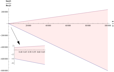
Figure 6: (color online). The dark area is the allowed range of $\frac{\textit{Im}(\beta)}{\textit{Re}(\beta)}$ in $\frac{m}{\Delta}$ parameter space in the case II, according to the experimental data of $\tan\delta$.

We find that the allowed region of $\frac{\textit{Im}(\beta)}{\textit{Re}(\beta)}$ onto our parameter space, in the case II, as

$$\frac{\textit{Im}(\beta)}{\textit{Re}(\beta)}\approx\leavevmode\nobreak\ -(4-\infty)\leavevmode\nobreak\ \text{and}\leavevmode\nobreak\ (1.2-\infty),$$ (28)

therefore, according Eq. (28)could write

$$\textit{Im}(\beta)\approx\leavevmode\nobreak\ -(4-\infty)\textit{Re}(\beta)\leavevmode\nobreak\ \text{and}\leavevmode\nobreak\ (1.2-\infty)\textit{Re}(\beta).$$ (29)

We obtain the allowed range of $\textit{Re}(\beta)$ in the two different regions which are specified in Eq. (28), as shown in the Figure 7, and the Figure8 respectively. As the pervious case, we do this by inserting the experimental data of $\sin^{2}\theta_{13}$ in the equation of $\sin^{2}\theta_{13}$ in Eq. (II.2) and mapping $\textit{Re}(\beta)$ onto our parameter space, in the case II.

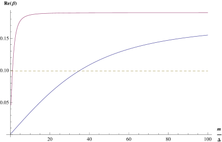
Figure 7: (color online). The range of $\textit{Re}(\beta)$ onto $\frac{m}{\Delta}$ our parameter space, according to the experimental data of $\sin^{2}\theta_{13}$ when $\textit{Im}(\beta)\approx\leavevmode\nobreak\ -(4-\infty)\textit{Re}(\beta)$. The area bellow the horizontal dashed line displays the allowed region of $\textit{Re}(\beta)$ in the case II within our model.

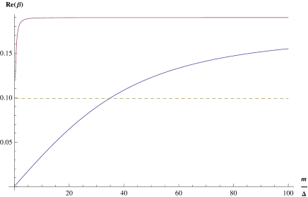
Figure 8: (color online). The range of $\textit{Re}(\beta)$ onto $\frac{m}{\Delta}$ our parameter space, according to the experimental data of $\sin^{2}\theta_{13}$ when $\textit{Im}(\beta)\approx\leavevmode\nobreak\ (1.2-\infty)\textit{Re}(\beta)$. The area bellow the horizontal dashed line displays the allowed region of $\textit{Re}(\beta)$ in the case II within our model.

As mentioned before, the allowed range of $\textit{Re}(\beta)$ must be bellow $0.099$; therefore, the area bellow the horizontal dashed line in the Figures 9 and, the Figure 10 displays the allowed range of $\textit{Re}(\beta)$ in the case II according to the two ranges of specified in  Eq. (29).

Afterwards, we map ${\textit{Im}(\beta)}$ based on Eq. (29) ,in the two different range of $\textit{Re}(\beta)$, as shown in the Figure 9 and, the Figure 10 respectively. We find that in the case II the obtained value of $\textit{Im}(\beta)$, is much greater than $|0.1|$, the red dashed line, which is not acceptable by the perturbation theory. Therefore, the obtained results in the case II, with $\Delta>0$ and $\textit{Re}(\alpha)>0$, are ruled out.

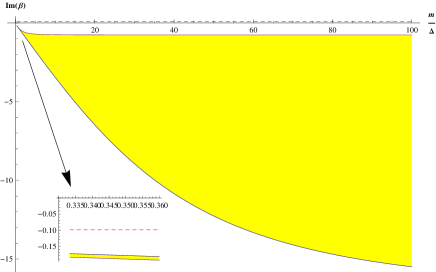
Figure 9: (color online). The range of $\textit{Im}(\beta)$ onto $\frac{m}{\Delta}$ our parameter space, according to the range of $\textit{Re}(\beta)$ when $\textit{Im}(\beta)\approx\leavevmode\nobreak\ -(4-\infty)\textit{Re}(\beta)$. The dark area displays the obtained region of $\textit{Im}(\beta)$ which is not allowed within our model because is greater than $|0.1|$ (the red dashed line).

Figure 10: (color online). The range of $\textit{Im}(\beta)$ onto $\frac{m}{\Delta}$ our parameter space, according to the range of $\textit{Re}(\beta)$ when $\textit{Im}(\beta)\approx\leavevmode\nobreak\ (1.2-\infty)\textit{Re}(\beta)$. The dark area displays the obtained region of $\textit{Im}(\beta)$ which is not allowed within our model because is greater than $|0.1|$ (the red dashed line).

IV Conclusion

We have studied the phenomenology of two-zero texture in the Majorana neutrino mass matrix with $A_{4}$ symmetry where the charged lepton mass matrix is diagonal. Therefore, there are seven viable two-zero textures. The seven viable textures are broadly categorized into two categories. To sum up, in general textures which are consistent with the experimental data as $M_{\nu}^{S_{1}}$, $M_{\nu}^{S_{2}}$, $M_{\nu}^{S_{7}}$ and textures which are not consistent with the experimental data as $M_{\nu}^{S_{3}}$, $M_{\nu}^{S_{5}}$, and their permutation symmetry ,as $M_{\nu}^{S_{4}}$, $M_{\nu}^{S_{6}}$ respectively .

We studied, the texture $M_{\nu}^{S_{7}}$, with $(\mu,\mu)$ and $(\tau,\tau)$ vanishing elements, which has both magic and $\mu-\tau$ symmetry. Therefore its mixing matrix is $U_{TBM}$, with $\theta_{13}\neq 0$, $\delta=0$, and $\theta_{23}=45^{\circ}$. Hence, we consider $M_{\nu}^{S_{7}}$ with the attendance of a small contribution as perturbation matrix by employing the perturbation method , which generates simultaneously a tiny $\delta m^{2}$ and small parameters in the neutrino mixing component, such as, $U_{13}$, ($\theta_{13}$ and $\delta$), and provides minor amendments to $\theta_{23}$. Therefore, CP violation is investigated.

We reproduce the texture $M_{\nu}^{S_{7}}$ as unperturbed mass matrix in the flavor basis which has a structure in which $\theta_{13}=0$, $\delta m^{2}=0$, $\theta_{23}=45^{\circ}$, and $\Delta m^{2}\neq 0$. We work on the diagonal mass matrix of the reproduced $M_{\nu}^{S_{7}}$ as unperturbed mass matrix in the mass basis which has degeneracy $m_{1}^{(0)}=m_{2}^{(0)}$.

Our perturbation mass matrix is symmetric and complex in the mass basis, and thereby, is non-Hermitian matrix. We obtain $\theta_{13}$, $\delta$ and, $\delta m^{2}$ that all could arise from a perturbation. The perturbation also affects the atmospheric mixing angle $\theta_{23}$. We have two different cases; in the case I, $\Delta$ and $\textit{Re}(\alpha)$ are negative while in the case II, both are positive.

We compare our results with the experimental data in each case; in the case I, we could obtain the allowed range of our parameter space, $\frac{m}{\Delta}$ and the complex elements of perturbation mass matrix $\alpha$, and $\beta$; then we check the accuracy of our work and our results by obtaining the magnitude of $\theta_{23}$ by the obtained allowed range of our parameters. We obtain $\theta_{23}\approx(41.81^{\circ}-43.96^{\circ})$ which is in complete agreement with the experimental data in Eq. (I) and shows the accuracy of our work. Moreover we predict the neutrino mass ordering is inverted in this case.

We fail to obtain an acceptable range for $\beta$ in the case II so this case is ruled out.

V Acknowledgments

We would like to thank the research office of the Qazvin Branch, Islamic Azad University.

References

- (1) J. Schechter and J. W. F. Valle, Neutrino masses in theories, Phys.Rev. D22 (1980) 2227.
- (2) H. Fritzsch and Z.Z. Xing, How to Describe Neutrino Mixing and CP Violation , Phys. Lett. B 517, 363 (2001) [hep-ph/0103242v2].
- (3) Particle Data Group, W.M. Yao et al., Review of Particle Physics , J. Phys. G 33, 1 (2006).
- (4) K. Abe et al. (T2K Collaboration), Precise Measurement of the Neutrino Mixing Parameter from Muon Neutrino Disappearance in an Off-Axis Beam, Phys. Rev. Lett. 112, 181801 (2014).
- (5) K. Abe et al. (T2K Collaboration), Observation of Electron Neutrino Appearance in a Muon Neutrino Beam, Phys. Rev. Lett. 112, 061802 (2014).
- (6) J. K. Ahn et al. (RENO Collaboration), Observation of Reactor Electron Antineutrino Disappearance in the RENO Experiment, Phys. Rev. Lett. 108, 191802 (2012).
- (7) Y. Abe et al. (Double Chooz Collaboration), Reactor electron antineutrino disappearance in the Double Chooz experiment, Phys. Rev. D 86, 052008 (2012).
- (8) F. P. An et al. (Daya Bay Collaboration), Spectral Measurement of Electron Antineutrino Oscillation Amplitude and Frequency at Daya Bay, Phys. Rev. Lett. 112, 061801 (2014).
- (9) B. Z. Hu (Daya Bay Collaboration), New results from the Daya Bay reactor neutrino experiment, arXiv:1402.6439.
- (10) F. Capozzi, G. L. Fogli, E. Lisi, A. Marrone, D. Montanino, and A. Palazzo, Status of three-neutrino oscillation parameters, circa 2013, Phys. Rev. D 89, 093018 (2014).
- (11) K. A. Olive, K. Nakamura, S. T. Petcov et al. (Particle Data Group Collaboration), Review of particle physics, Chin. Phys. C 38, 090001 (2014).
- (12) P. F. Harrison et al., Tri-Bimaximal Mixing and the Neutrino Oscillation Data, Phys. Lett. B530, 167 (2002) [hep-ph/0202074v1].
- (13) P. F. Harrison, D. H. Perkins, and W. G. Scott, Tri-bimaximal mixing and the neutrino oscillation data, Phys. Lett. B 530, 167 (2002).
- (14) P. H. Frampton , T. W. Kephart and S. Mat-suzaki, Simplified renormalizable T model for tribimaximal mixing and Cabibbo angle, Phys. Rev. D 78 , 073004 (2008) [hep-ph/0807.4713].
- (15) G. Altarelli and F. Feruglio, Tri-Bimaximal Neutrino Mixing, A4 and the Modular Symmetry, Nucl. Phys. B 741 , 215 (2006) [hep-ph/0512103].
- (16) B. Grinstein and M. Trott, [hep-ph/1203.4410]; S. F. King, Parametrizing the lepton mixing matrix in terms of deviations from tri-bimaximal mixing, Phys. Lett. B 659, 244 (2008) [hep-ph/0710.0530]; S. Pakvasa, W. Rodejohann, T. Weiler, Unitary Parametrization of Perturbations to Tribimaximal Neutrino Mixing, Phys. Rev. Lett. 100, 111801 (2008); C. H. Albright, A. Dueck, W. Rodejohann, Possible Alternatives to Tri-bimaximal Mixing, Eur. Phys. J. C 70, 1099-1110 (2010) [hep-ph/1004.2798v1]; S. Boudjemaa and S. F. King, Deviations from Tri-bimaximal Mixing: Charged Lepton Corrections and Renormalization Group Running, Phys. Rev. D 79, 033001 (2009) [hep-ph/0808.2782]; S. Goswami, S. T. Petcov, S. Ray and W. Rodejohann, Large Ue3 and Tri-bimaximal Mixing, Phys. Rev. D 80, 053013 (2009) [hep-ph/0907.2869]; D. Meloni, F. Plentinger and W. Winter, Perturbing exactly tri-bimaximal neutrino mixings with charged lepton mass matrices, Phys. Lett. B 699, 354 (2011) [hep-ph/1012.1618]; Sumit K. Garg, Consistency of perturbed Tribimaximal, Bimaximal and Democratic mixing with Neutrino mixing data , Nucl. Phys. B931C (2018) 469-505; D. Marzocca, S. T. Petcov, A. Romanino and M. Spinrath, Sizeable è13 from the Charged Lepton Sector in SU(5), (Tri-)Bimaximal Neutrino Mixing and Dirac CP Violation, JHEP 1111, 009 (2011) [hep-ph/1108.0614]; G. Altarelli and F. Feruglio, Tri-Bimaximal Neutrino Mixing, A4 and the Modular Symmetry, Nucl. Phys. B 741, 215 (2006) [hep-ph/0512103]; F. Bazzocchi, S. Morisi and M. Picariello, Embedding A4 into left-right flavor symmetry: Tribimaximal neutrino mixing and fermion hierarchy, Phys. Lett. B 659, 628 (2008) [hep-ph/0710.2928]; E. Ma and D. Wegman, Nonzero theta(13) for neutrino mixing in the context of A(4) symmetry, Phys. Rev. Lett. 107, 061803 (2011) [hep-ph/1106.4269]; S. Gupta, A. S. Joshipura and K. M. Patel, Minimal extension of tri-bimaximal mixing and generalized Z2 X Z2 symmetries, Phys. Rev. D 85, 031903 (2012) [hep-ph/1112.6113]; B. Adhikary, B. Brahmachari, A. Ghosal, E. Ma and M. K. Parida, A4 symmetry and prediction of Ue3 in a modified Altarelli-Feruglio model, Phys. Lett. B 638, 345 (2006) [hep-ph/0603059]; E. Ma, Near Tribimaximal Neutrino Mixing with Ä(27) Symmetry, Phys. Lett. B 660, 505 (2008) [hep-ph/0709.0507]; F. Plentinger, G. Seidl and W. Winter, Group space scan of flavor symmetries for nearly tribimaximal lepton mixing, JHEP 0804, 077 (2008) [hep-ph/0802.1718]; N. Haba, R. Takahashi, M. Tanimoto and K. Yoshioka, Tri-bimaximal Mixing from Cascades, Phys. Rev. D 78, 113002 (2008) [hep-ph/0804.4055]; S. -F. Ge, D. A. Dicus and W. W. Repko, Residual Symmetries for Neutrino Mixing with a Large theta13 and Nearly Maximal deltaD, Phys. Rev. Lett. 108, 041801 (2012) [hep-ph/1108.0964]; T. Araki and Y. F. Li, Q6 flavor symmetry model for the extension of the minimal standard model by three right-handed 15 sterile neutrinos, Phys. Rev. D 85, 065016 (2012) [hep-ph/1112.5819].
- (17) E. Ma and G. Rajasekaran, Phys. Rev. D64, 113012 (2001).
- (18) Ernest Ma, Aspects of the Tetrahedral Neutrino Mass Matrix, Phys.Rev.D72:037301,(2005).
- (19) G. Altarelli and F. Feruglio, Discrete flavor symmetries and models of neutrino mixing, Rev. Mod. Phys. 82, 2701 (2010).
- (20) M. Hirsch, A. S. Joshipura, S. Kaneko, and J.W. F. Valle, Predictive Flavour Symmetries of the Neutrino Mass Matrix, Phys. Rev. Lett. 99, 151802 (2007).
- (21) G. Altarelli and F. Feruglio, Tri-bimaximal neutrino mixing, A(4) and the modular symmetry, Nucl. Phys. B741, 215 (2006).
- (22) G. Altarelli and D. Meloni, A simplest A4 model for tribimaximal neutrino mixing, J. Phys. G 36, 085005 (2009).
- (23) K. M. Parattu and A. Wingerter, Tribimaximal mixing from small groups, Phys. Rev. D 84, 013011 (2011).
- (24) S. F. King and C. Luhn, A4 models of tri-bimaximal-reactor mixing, J. High Energy Phys. 03 (2012) 036.
- (25) G. Altarelli, F. Feruglio, L. Merlo, and E. Stamou, Discrete flavour groups, and lepton flavour violation, J. High Energy Phys. 08 (2012) 021.
- (26) G. Altarelli, F. Feruglio, and L. Merlo, Tri-bimaximal neutrino mixing and discrete flavour symmetries, Fortschr. Phys. 61, 507 (2013).
- (27) P. M. Ferreira, L. Lavoura, and P. O. Ludl, A new A4 model for lepton mixing, Phys. Lett. B 726, 767 (2013).
- (28) J. Barry and W. Rodejohann, Deviations from tribimaximal mixing due to the vacuum expectation value misalignment in models, Phys. Rev. D 81, 093002 (2010); 81, 119901(E) (2010).
- (29) Y. H. Ahn and S. K. Kang, Non-zero and CP violation in a model with flavor symmetry, Phys. Rev. D 86, 093003 (2012).
- (30) H. Ishimori and E. Ma, New simple A4 neutrino model for nonzero and large , Phys. Rev. D 86, 045030 (2012).
- (31) E. Ma, A. Natale, and A. Rashed, Scotogenic A4 neutrino model for nonzero and large , Int. J. Mod. Phys. A 27, 1250134 (2012).
- (32) D. N. Dinh, N. A. Ky, P. Q. V.n, and N. T. H. Van, in 2nd International Workshop on Theoretical and Computational Physics (IWTCP-2), Ban-Ma-Thuat, July, 2014 (2014); A prediction of for a normal neutrino mass ordering in an extended standard model with an flavour symmetry, J. Phys. Conf. Ser. 627, 012003 (2015).
- (33) D. N. Dinh, N. A. Ky, P. Q. Vãn, and N. T. H. Vân, A seesaw scenario of an flavor symmetric standard model, arXiv:1602.07437.
- (34) P. F. de Salas, D. V. Forero, S. Gariazzo, P. Martínez-Miravé, O. Mena, C. A. Ternes, M. Tórtola, J. W. F. Valle, 2020 Global reassessment of the neutrino oscillation picture, J. High Energ. Phys. 2021, 71 (2021).
- (35) Razzaghi, N.; Rasouli, S.M.M.; Parada, P.; Moniz, P. Two-Zero Textures Based on A4 Symmetry and Unimodular Mixing Matrix. Symmetry 2022, 14, 2410.
- (36) F. Vissani, J. High Energy Phys. 9811 (1998) 025; E.K.Akhmedov, Phys. Lett. B 467 (1999) 95; M. Lindner, W. Rodejohann, J. High Energy Phys. 0705 (2007) 089; D. Aristizabal Sierra, I. de Medeiros Varzielas, E. Houet, Phys. Rev. D 87 (2013) 093009; T. Araki, Prog. Theor. Exp. Phys. 2013 (2013) 103B02; M.-C. Chen, J. Huang, K.T. Mahanthappa, A.M. Wijangco, J. High Energy Phys. 1310 (2013) 112; L.J. Hall, G.G. Ross, J. High Energy Phys. 1311 (2013) 091; Jiajun Liao, D. Marfatia, K. Whisnant, Phys. Rev. D 92, 073004 (2015) ; Sumit K. Garg, Nucl. Phys. B931C (2018) 469-505.
- (37) C.S. Lam, Magic Neutrino Mass Matrix and the Bjorken-Harrison-Scott Parameterization, Phys.Lett. B640 (2006) 260-262[ arXiv:hep-ph/0606220v2].
- (38) Radha Raman Gautam, Sanjeev Kumar, Zeros in the magic neutrino mass matrix, PHYSICAL REVIEW D 94, 036004 (2016).
- (39) S.Weinberg, Trans. New York Acad. Sci. 38, 185 (1977); F.Wilczek and A. Zee, Phys. Lett. 70B, 418 (1977); H. Fritzsch, Phys. Lett. 70B, 436 (1977); Phys. Lett. 73B, 317 (1978); Nucl. Phys. B155, 18 (1979).
- (40) H. Fritzsch and Z.Z. Xing, Prog. Part. Nucl. Phys. 45, 1 (2000); Z.Z. Xing, Int. J. Mod. Phys. A 19, 1 (2004); arXiv:hep-ph/0406049.
- (41) Paul H. Frampton, Sheldon L. Glashow and Danny Marfatia, Phys. Lett. B 536, 79 (2002),hep-ph/0201008. 20
- (42) Zhi-zhong Xing, Phys. Lett. B 530, 159 (2002), hep-ph/0201151; H. Fritzsch, Z. Z. Xing, Phys. Lett. B 517 (2001) 363-368, arXiv: hep ph/0103242.
- (43) Bipin R. Desai, D. P. Roy and Alexander R. Vaucher, Mod. Phys. Lett. A 18, 1355 (2003), hep-ph/0209035; A. Merle, W. Rodejohann, Phys. Rev. D 73, 073012 (2006), hep ph/0603111; S. Dev, Sanjeev Kumar, S. Verma and S. Gupta, Nucl. Phys. B 784, 103-117 (2007), hep-ph/0611313; S. Dev, S. Kumar, S. Verma and S. Gupta, Phys. Rev. D 76, 013002 (2007), hep-ph/0612102; M. Randhawa, G. Ahuja, M. Gupta, Phys. Lett. B 643, 175-181 (2006), hep- ph/0607074; G. Ahuja, S.Kumar, M. Randhawa, M. Gupta, S. Dev, Phys. Rev. D 76, 013006 (2007), hep-ph/0703005; S. Kumar, Phys. Rev. D 84, 077301 (2011), arXiv: 1108.2137 [hep-ph]; P. O. Ludl, S. Morisi, E. Peinado, Nucl. Phys. B 857, 411 (2012), arXiv: 1109.3393 [hep-ph]; Manmohan Gupta, Gul- sheen Ahuja, Int. J. Mod. Phys. A, 27, 1230033 (2012), arXiv:1302.4823 [hep- ph]; D.Meloni, G. Blankenburg, Nucl. Phys. B 867, 749 (2013), arXiv:1204.2706 [hep-ph]; W. Grimus, P. O. Ludl, J. Phys. G40, 055003 (2013), arXiv:1208.4515 [hep-ph]; S. Sharma, P. Fakay, G. Ahuja and M. Gupta arXiv: 1402.1598 [hep- ph]; P. O. Ludl, W. Grimus, arXiv:1406.3546v1 [hep-ph]; H. Fritzsch, Zhi-zhong Xing, S. Zhou, JHEP 1109, 083 (2011), arXiv: 1108.4534 [hep-ph]; Madan Singh, Gulsheen Ahuja, Manmohan Gupta, Prog. Theor. Exp. Phys. (PTEP) 2016 (12): 123B 08, arXiv: 1603.08083 [hep-ph]; Madan Singh, Adv. High Energy Phys. 2018(2018) 2863184, arXiv: 1803.10735[hep-ph].
- (44) C. Hagedorn and W. Rodejohann, JHEP 0507, 034 (2005).
- (45) X. Liu, S. Zhou, Int. J. Mod. Phys. A 28 (2013) 1350040.
- (46) E. I. Lashin and N. Chamoun, Phys. Rev. D85, 113011 (2012), arXiv: 1108.4010 [hep-ph].
- (47) H. Fritzsch, Z.-z. Xing, and S. Zhou, J. High Energy Phys. 09 (2011) 083.
- (48) Razzaghi, N.; Rasouli, S.M.M.; Parada, P.; Moniz, P. Generating CP Violation from a Modified Fridberg-Lee Model. Universe 2022, 8, 448.
- (49) Aghanim, N.; Akrami, Y.; Ashdown, M.; Aumont, J.; Baccigalupi, C.; Ballardini, M.; Banday, A.J.; Barreiro, R.B.; Bartolo, N.; Basak, S.; et al. Planck 2018 results-VI. Cosmological parameters. Astron. Astrophys. 2020, 641, A6. …