Principled Multi-Aspect Evaluation Measures of Rankings

Abstract.

Information Retrieval evaluation has traditionally focused on defining principled ways of assessing the relevance of a ranked list of documents with respect to a query. Several methods extend this type of evaluation beyond relevance, making it possible to evaluate different aspects of a document ranking (e.g., relevance, usefulness, or credibility) using a single measure (multi-aspect evaluation). However, these methods either are (i) tailor-made for specific aspects and do not extend to other types or numbers of aspects, or (ii) have theoretical anomalies, e.g. assign maximum score to a ranking where all documents are labelled with the lowest grade with respect to all aspects (e.g., not relevant, not credible, etc.).

We present a theoretically principled multi-aspect evaluation method that can be used for any number, and any type, of aspects. A thorough empirical evaluation using up to $5$ aspects and a total of $425$ runs officially submitted to $10$ TREC tracks shows that our method is more discriminative than the state-of-the-art and overcomes theoretical limitations of the state-of-the-art.

1. Introduction

Multi-aspect evaluation is a task in Information Retrieval (IR) evaluation where the ranked list of documents returned by an IR system in response to a query is assessed in terms of not only relevance, but also other aspects (or dimensions) such as credibility or usefulness. Generally, there are two ways to conduct multi-aspect evaluation: (1) evaluate each aspect separately using any appropriate single-aspect evaluation measure (e.g., AP, NDCG, F1), and then aggregate the scores across all aspects into a single score; or (2) evaluate all aspects at the same time using any appropriate multi-aspect evaluation measure (Amigó et al., 2018b; Lioma et al., 2017; Tang and Yang, 2017). An advantage of the aggregating option (1) is that it is easy to implement using evaluation measures that are readily available and well-understood in the community. Its disadvantage is that it is not guaranteed that all aspects will have similar distributions of labels, and aggregating across wildly different distributions can give odd results (Lioma et al., 2019). The second way of doing multi-aspect evaluation is to use a single multi-aspect evaluation measure. The problem here is that few such evaluation measures exist, and most of them are defined for specific aspects and do not generalise to other types/numbers of aspects (see $\S$2).

Motivated by the above, we contribute a novel multi-aspect evaluation method that works with any type and number of aspects, and avoids the above problems. Given a ranked list, where documents are labelled with multiple aspects, our method, Total Order Multi-Aspect (TOMA) evaluation, first defines a preferential order (formally weak order relation) among documents with multiple aspect labels, and then aggregates the document labels across aspects to obtain a ranking of aggregated aspect labels, which can be evaluated by any single-aspect evaluation measure, such as Normalized Discounted Cumulated Gain (NDCG) or Average Precision (AP). Simply put, instead of evaluating each aspect separately and then aggregating their scores, we first aggregate the aspect labels and then evaluate the ranked list of documents. We do this in a way that provides several degrees of freedom: our method can be used with any number and type of aspects, can be instantiated with any binary or graded, set-based or rank-based evaluation measure, and can accommodate any granularity in the importance of each aspect or label, but still ensures, by definition, that the preference order among multi-aspect documents is not violated, and that the final measure score will meet some common requirements, i.e., the minimum (worst) score being $0$ and the maximum (perfect) score being $1$. We validate this empirically ($\S$4) and theoretically ($\S$4.2).

2. Related Work

Multi-aspect evaluation measures for IR have been studied for different tasks and aspects, starting from the INEX initiative with relevance and coverage (Kazai et al., 2004). Since then, measures have been proposed to evaluate relevance and novelty or diversity, such as $\alpha$-NDCG (Clarke et al., 2008), MAP-IA (Agrawal et al., 2009) and IA-ERR (Chapelle et al., 2009); relevance, novelty and the amount of user effort, such as nCT (Tang and Yang, 2017); relevance, redundancy and user effort, such as RBU (Amigó et al., 2018b); relevance and understandability, such as uRBP (Zuccon, 2016) and the Multidimensional Measure (MM) framework (Palotti et al., 2018); and relevance and credibility, such as NLRE, NGRE, nWCS, Convex Aggregating Measure (CAM) and WHAM (Lioma et al., 2017). All these measures have limitations; we describe these next.

Firstly, except for RBU, none of the above measures are based on a formal framework. They are defined as stand-alone tools to assess the effectiveness of a ranked list of documents. This means that, even if the measure can assess the effectiveness of an input ranking, the order induced by the measure over the space of input rankings is not well-defined. Hence, there is no canonical ideal ranking that is well-defined or easy to compute, e.g., for $\alpha$-NDCG, the computation of the ideal ranking is equivalent to a minimal vertex covering problem (Clarke et al., 2008), an NP-complete problem, while for CT and nCT, computing the ideal ranking is equivalent to the minimum edge dominating set problem (Tang and Yang, 2017), an NP-hard problem. Computationally better ways of comparing to an ideal ranking can be devised using graded similarity—so-called effectiveness levels to an ideal ranking using Rank-Biased Overlap (Clarke et al., 2020c, b, 2021), but this approach requires defining a (set of) ideal ranking(s), which has not appeared for multi-aspect ranking prior to the present paper.

Evaluation measures that do not compare against an ideal ranking may be harder to interpret or problematic. DCG is not upper bounded by $1$, thus different topics are not weighted equally and scores are not comparable. Failing to compare against the ideal ranking is problematic in multi-aspect evaluation: $\alpha$-NDCG allows systems to reach scores greater than $1$, which is supposed to be the score of the perfect system. With NLRE and NGRE, a system that retrieves no relevant or credible documents has error =$0$, i.e., achieves the best score, because the relative order of pairs of documents is always correct (Lioma et al., 2019). Similarly, nWCS can reach the perfect score of $1$, even if no relevant or credible documents are retrieved, since the normalization is computed with a re-ranking of the input ranking, instead of the ideal ranking.

Both uRBP and RBU have a different problem: to reach the perfect score of $1$, a system must retrieve an infinite number of relevant and understandable documents, even if those documents are not available in the collection. CAM and WHAM use the weighted arithmetic and weighted harmonic mean of any IR measure computed with respect to relevance and credibility independently. Therefore, depending on the distribution of labels across the aspects, it can be impossible for any system to reach the perfect score (see $\S$ 4.2).

Secondly, most of the above multi-aspect evaluation measures are defined for specific contexts and with a limited set of aspects, e.g., novelty, diversity, credibility and understandability, thus they cannot deal with a more general scenario and a variable number of aspects. For RBU, even though a formal framework is defined, its formulation specifies only diversity and redundancy constraints, which cannot be applied to a general set of aspects. This inability to generalise to more/other types of aspects means that, if a system must be evaluated with respect to a new aspect, the measure needs to be properly adapted. This can be easily done for some measures, e.g., CAM, WHAM, and nWCS, but the lack of a formal framework behind them may lead to odd results, e.g., extending NLRE to $3$ aspects returns a score distribution compressed towards $0$, preventing the rankings to be evaluated in a fair way (Lioma et al., 2019).

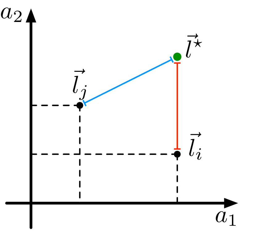
(a) Distance order.

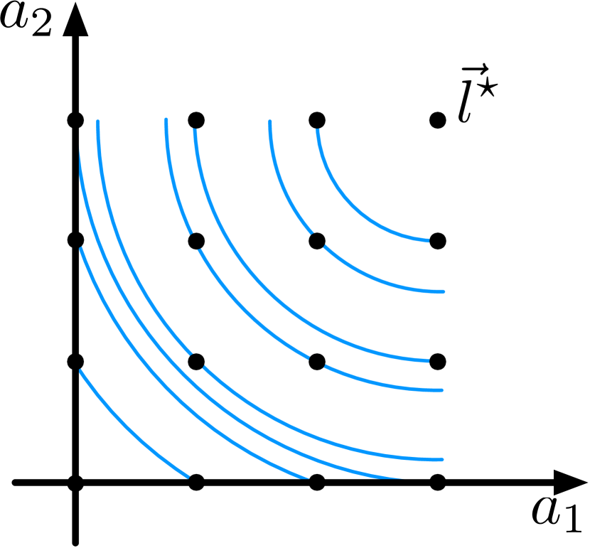
(b) Euclidean distance.

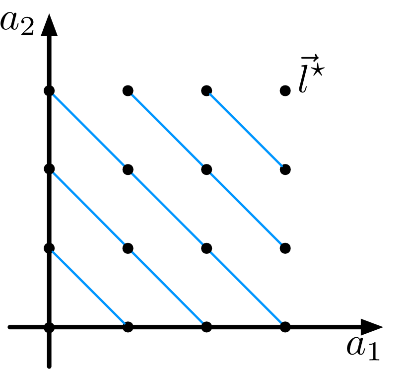
(c) Manhattan distance.

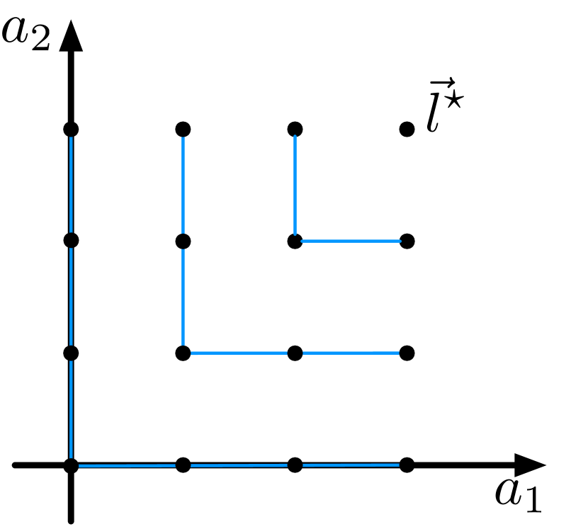
(d) Chebyshev distance.

Figure 1. Example with two aspects $a_{1}$ and $a_{2}$. Each point is a tuple of labels. The best label $\mathbf{l^{\star}}$ is in the top right. The distance between tuples of labels and $\mathbf{l^{\star}}$ defines a weak order relation. Blue lines connect tuples of labels at the same distance from $\mathbf{l^{\star}}$.

3. TOMA Framework

We formalize the problem and our proposed methodology: we explain why reasoning in terms of multiple aspects leads to a partial order relation among documents ($\S$ 3.1); how we complete the partial order relation with the distance order ($\S$ 3.2); and how to use the distance order with state-of-the-art IR evaluation measures ($\S$ 3.3).

3.1. Formalization of the Problem

Let $A=\{a_{1},\ldots,a_{n}\}$ be a set of aspects; each aspect $a\in A$ has a non-empty set of labels $L_{a}=\{l_{0}^{a},\ldots,l_{K_{a}}^{a}\}$ and an order relation $\prec_{a}$ such that: $l_{0}^{a}\prec_{a}l_{1}^{a}\prec_{a}\cdots\prec_{a}l_{K_{a}}^{a}$, e.g., we may have $2$ aspects $A=\{\text{relevance},\text{correctness}\}$, with the set $L_{r}=\{\texttt{nr},\texttt{mr},\texttt{fr},\texttt{hr}\}$ (non-relevant, marginally relevant, fairly relevant, highly relevant) ordered as: $\texttt{nr}\prec_{r}\texttt{mr}\prec_{r}\texttt{fr}\prec_{r}\texttt{hr}$; and the set $L_{c}=\{\texttt{nc},\texttt{pc},\texttt{c}\}$ (non-correct, partially correct, correct) ordered as: $\texttt{nc}\prec_{c}\texttt{pc}\prec_{c}\texttt{c}$. Let $D$ be the set of documents and $T$ the set of topics. Each document $d\in D$ is mapped to a ground truth vector $\textrm{GT}(d,t)=(l_{1},\ldots,l_{n})\in L_{a_{1}}\times\cdots\times L_{a_{n}}$ that contains the “true” label of $d$ for each aspect, e.g., a document may have $\textrm{GT}(d,t)=(\textrm{highly relevant},\textrm{non-correct})$.

In IR, given a topic $t$, the objective is to rank documents in $D$ such that for the documents $d^{\prime},d\in D$, if $d^{\prime}$ is ranked before $d$, then $\textrm{GT}(d,t)\preceq_{*}\textrm{GT}(d^{\prime},t)$ for a given order relation $\preceq_{*}$. When there is only one aspect $A=\{a\}$, one can use $\prec_{a}$, the order on the set of labels $L_{a}$, to induce a weak order on $D$ and decide if $d^{\prime}$ should be ranked before $d$. If only relevance is assessed, we consider the relation induced by relevance labels, i.e., documents labelled “highly relevant” should be ranked before “fairly/marginally relevant” and “non-relevant” documents. Applying this approach to multiple aspects requires reasoning about orderings of tuples of labels with different aspects, e.g., for documents $d^{\prime},d\in D$, such that $\textrm{GT}(d^{\prime},t)=(\text{highly relevant},\text{correct})$ and $\textrm{GT}(d,t)=($marginally relevant, correct$)$, it is reasonable to rank $d^{\prime}$ before $d$.

Indeed, there is one unequivocal way of deeming one document better than another, and this is if document $d^{\prime}$ has better labels than document $d$ for every aspect: if for $\textrm{GT}(d,t)=(l_{1},\ldots,l_{n})$ and $\textrm{GT}(d^{\prime},t)=(l_{1}^{\prime},\ldots,l_{n}^{\prime})$ we have $l_{i}\preceq_{a_{i}}l_{i}^{\prime}$ for all $i\in\{1,\ldots,n\}$, then any document labeled $(l_{1}^{\prime},\ldots,l_{n}^{\prime})$ is better or equal than any document labelled $(l_{1},\ldots,l_{n})$ and should occur before it in a “good” ranking. We denote this order relation by $\textrm{GT}(d,t)\sqsubseteq\textrm{GT}(d^{\prime},t)$.

The order relation $\sqsubseteq$ leads to a partial instead of a total order, i.e., there are documents that are not comparable, e.g., if $d^{\prime}$ is now highly relevant and partially correct, the final ranking is not clear: should one promote $d^{\prime}$ (more relevant) or $d$ (more correct)? This is an example of documents that are not comparable, so we have $\textrm{GT}(d,t)\not\sqsubseteq\textrm{GT}(d^{\prime},t)$ and $\textrm{GT}(d^{\prime},t)\not\sqsubseteq\textrm{GT}(d,t)$, and the choice of whether $d^{\prime}$ is preferred to $d$ may lie on the intended application.

A partial order relation and the presence of not comparable documents imply that it is not possible to univocally rank the documents in $D$. If we could “complete” the partial order with a total order, or at least a weak order, we could rank documents and define an ideal ranking, where for any $d^{\prime},d\in D$, the order relation determines the rank position of $d^{\prime}$ and $d$. So, before tackling the problem of evaluating a ranked list of documents in a multi-aspect way, we build such an order relation. This is detailed next.

3.2. The distance order

We now explain how to obtain a weak order relation from the partial order relation $\sqsubseteq$. Consider the Cartesian product of all sets of labels $L=L_{a_{1}}\times\cdots\times L_{a_{n}}$. An element $\mathbf{l}\in L$ is a tuple of labels $\mathbf{l}=(l_{1},\dots,l_{n})$. The total order relation will be denoted by $\preceq_{*}$ and it will be a weak order relation on $L$, i.e., a total binary relation that is reflexive and transitive, but not necessarily anti-symmetric (Ferrante et al., 2015, 2017, 2019b). This weak order allows all tuples of labels to be compared, i.e., for any two $\mathbf{l},\mathbf{l}^{\prime}\in L$ we will have $\mathbf{l}^{\prime}\preceq_{*}\mathbf{l}$ and/or $\mathbf{l}\preceq_{*}\mathbf{l}^{\prime}$. Consequently, all documents will be comparable through their tuple of labels.

We require that the weak order relation $\preceq_{*}$ respects the partial order relation $\sqsubseteq$:

(1) $$\forall\ \mathbf{l},\mathbf{l}^{\prime}\in L\textrm{ we have }\mathbf{l}\sqsubseteq\mathbf{l}^{\prime}\Rightarrow\mathbf{l}\preceq_{*}\mathbf{l}^{\prime}$$

This means that, for comparable documents, the partial order relation and the weak order relation rank documents in the same way. Moreover the weak order relation allows to rank even those documents that are not comparable with the partial order relation.

To define $\preceq_{*}$, we embed the tuples of labels in the Euclidean space and derive the weak order $\preceq_{*}$ using known distance functions. Let $g$ be an embedding function that maps tuples of labels in Euclidean space $\mathcal{L}=\mathbb{R}^{n}$: $g(\mathbf{l})=g(l_{1},\ldots,l_{n})=(g_{a_{1}}(l_{1}),\ldots,g_{a_{n}}(l_{n}))$. We assume that for each $a\in A$, $g_{a}$ is a non-decreasing map, i.e., for any $l,l^{\prime}\in L_{a}$ if $l\preceq_{a}l^{\prime}$ then $g_{a}(l)\leq g_{a}(l^{\prime})$. Intuitively, $g_{a}$ assigns a number to each label, which allows to represent tuples of labels in the Euclidean space. We illustrate in $\S$3.4 how the embedding function $g$ affects the final ranking of documents.

Through the embedding function $g$, each tuple of labels $\mathbf{l}$ is represented by a point in the Euclidean space $\mathcal{L}$ denoted by $\vec{l}=g(\mathbf{l})$. We define the best label tuple as the tuple of labels $\mathbf{l^{\star}}$ whose coordinates are the best label for each aspect, $\mathbf{l^{\star}}=(l_{K_{a_{1}}},\ldots,l_{K_{a_{n}}})$. The idea is to treat $\mathbf{l^{\star}}$ as the maximum element and use the distance from this maximum element to define the desired weak order relation; e.g., for two aspects $a_{1}$ and $a_{2}$, each tuple of labels is represented as a point in the Euclidean plane, and the best label $\mathbf{l^{\star}}$ is represented by the topmost and right-most point (see Fig. 1(a)). Then, given two documents $d$ and $d^{\prime}$, $d$ is ranked before $d^{\prime}$ if $\textrm{GT}(d,t)$ is closer to the best label than $\textrm{GT}(d^{\prime},t)$.

We formally define the distance order as the following relation:

(2) $$\mathbf{l}\preceq_{*}\mathbf{l^{\prime}}\ \iff\ \text{Dist}(\vec{l},\vec{l^{\star}})\geq\text{Dist}(\vec{l^{\prime}},\vec{l^{\star}})$$

where $\text{Dist}\colon\mathcal{L}\times\mathcal{L}\to[0,+\infty[$ is any function such that $\text{Dist}(\vec{l}^{\star},\vec{l}^{\star})=0$. The relation $\preceq_{*}$ is a weak order: all $\mathbf{l}$, $\mathbf{l^{\prime}}$ are comparable because $\text{Dist}(\vec{l},\vec{l^{\star}})$ is defined for all $\mathbf{l}$, and as $\geq$ is reflexive and transitive on $[0,+\infty[$, the relation $\preceq_{*}$ is reflexive and transitive (but not necessarily antisymmetric). Since the distance order is a weak order, it allows to deem items “equally good” when it is impossible or undesirable to impose a strict total order. Thus we write:

(3) $$\mathbf{l}=_{*}\mathbf{l^{\prime}}\ \iff\ \text{Dist}(\vec{l},\vec{l^{\star}})=\text{Dist}(\vec{l^{\prime}},\vec{l^{\star}})$$

which means that $\vec{l}$ and $\vec{l^{\prime}}$ are at the same distance from $\vec{l}^{\star}$.

Note that the distance order can be tailored: we may instantiate Dist with any valid distance function. We illustrate this in Fig. 1(b)-1(d) with Euclidean (order relation $\preceq_{2}$), Manhattan (order relation $\preceq_{1}$), and Chebyshev (order relation $\preceq_{\infty}$). With these choices of Dist, the distance order defined in Eq. (2)-(3) respects the partial order $\sqsubseteq$, which means that it satisfies the requirement in Eq. (1) because $g_{a}$ is a non decreasing map (a proof is provided in the online appendix).

3.3. Integration with IR measures

Next we integrate the distance order with known IR measures such as AP or NDCG. The binary relation $=_{*}$ in Eq. (3) is an equivalence relation. Given a tuple of labels $\mathbf{l}\in L$, its equivalence class $[\mathbf{l}]_{*}$ is the set of all tuples of labels with equal distance from the best label $[\mathbf{l}]_{*}=\{\mathbf{l^{\prime}}\in L\colon\text{Dist}(\vec{l^{\prime}},\vec{l^{\star}})=\text{Dist}(\vec{l},\vec{l^{\star}})\}$.

Inducing the relation defined in Eq. (2) on the set of documents $D$ allows to rank documents by their membership to each equivalence class, which corresponds to the distance of their tuple of labels to the best label. We place closest to the top of the ranking documents whose equivalence class is closest to the best label, and vice versa.

To combine the distance order with IR measures we map each equivalence class (set of tuple of labels), to a non negative integer. This is similar to what happens with single-aspect evaluation, where each label is mapped to a weight: e.g., with $4$ relevance labels, we can compute NDCG with equi-spaced relevance weights $\{0,1,2,3\}$ (Järvelin and Kekäläinen, 2002) or exponential weights $\{0,2,4,8\}$ (Burges et al., 2005). We define a weight function $W\colon L\to\mathbb{N}_{0}^{+}$ as a map such that the order relation $\preceq_{*}$ is preserved:

(4) $$\forall\ \mathbf{l},\mathbf{l^{\prime}}\in L\colon\mathbf{l}\preceq_{*}\mathbf{l^{\prime}}\implies W(\mathbf{l})\leq W(\mathbf{l^{\prime}})$$

where the constraint in Eq. (4) entails that $W$ is a non-decreasing function with respect to the weak order $\preceq_{*}$ on the set of tuples of labels. This means that $W$ can return different integers for each equivalence class, but also the same integer for different equivalence classes, i.e., $0$ and $1$, whenever we need to compute a binary single-aspect IR measure as AP.

To summarize, our TOMA method has $3$ steps:

1. We embed tuples of labels into elements of Euclidean space, and we derive the weak order $\preceq_{*}$ using a distance function;

2. We define an adjustable weight function $W$ that preserves $\preceq_{*}$ and maps each tuple of labels to a single integer weight (this allows to aggregate tuple of labels so that better documents can be given greater weight);

3. Having such a weak order and the weight function $W$, any existing single-aspect IR evaluation measure can be used to assess the quality. Thus, we choose a single-aspect evaluation measure $\mu$ and compute the final evaluation score as $M=\mu\circ W\colon M(r_{t})=\mu(W(\textrm{GT}(d_{1},t)),\ldots,W(\textrm{GT}(d_{N},t)))$, where $r_{t}$ is a ranked list of documents.

The above is compatible with any number and type of aspect.

3.4. Example

Table 1. Final ordering of tuples of labels embedded in the Euclidean space. Relevance labels are always embedded in the same mapping (under Relevance). We use different mappings for correctness labels (under Correctness). Tuples that are relevant and not correct (high-traffic fake news) are in red.

Relevance	Correctness	Distance	Order among Tuples of Labels
$\{0,1,2,3\}$	$\{0,3/2,3\}$	Euclidean	$(3,3)\preceq_{*}(2,3)\preceq_{*}(3,3/2)\preceq_{*}(2,3/2)\preceq_{*}(1,3)\preceq_{*}(1,3/2)\preceq_{*}\mathbin{{\color[rgb]{0.86328125,0.078125,0.234375}(3,0)}}\preceq_{*}\mathbin{{\color[rgb]{0.86328125,0.078125,0.234375}(2,0)}}\preceq_{*}\mathbin{{\color[rgb]{0.86328125,0.078125,0.234375}(1,0)}}\preceq_{*}(0,0)$
		Manhattan	$(3,3)\preceq_{*}(2,3)\preceq_{*}(3,3/2)\preceq_{*}(1,3)\preceq_{*}(2,3/2)\preceq_{*}\mathbin{{\color[rgb]{0.86328125,0.078125,0.234375}(3,0)}}\preceq_{*}(1,3/2)\preceq_{*}\mathbin{{\color[rgb]{0.86328125,0.078125,0.234375}(2,0)}}\preceq_{*}\mathbin{{\color[rgb]{0.86328125,0.078125,0.234375}(1,0)}}\preceq_{*}(0,0)$
		Chebyshev	$(3,3)\preceq_{*}(2,3)\preceq_{*}(3,3/2)=_{*}(2,3/2)\preceq_{*}(1,3)=_{*}(1,3/2)\preceq_{*}\mathbin{{\color[rgb]{0.86328125,0.078125,0.234375}(3,0)}}=_{*}\mathbin{{\color[rgb]{0.86328125,0.078125,0.234375}(2,0)}}=_{*}\mathbin{{\color[rgb]{0.86328125,0.078125,0.234375}(1,0)}}=_{*}(0,0)$
$\{0,1,2,3\}$	$\{0,1,2\}$	Euclidean	$(3,2)\preceq_{*}(3,1)=_{*}(2,2)\preceq_{*}(2,1)\preceq_{*}\mathbin{{\color[rgb]{0.86328125,0.078125,0.234375}(3,0)}}=_{*}(1,2)\preceq_{*}\mathbin{{\color[rgb]{0.86328125,0.078125,0.234375}(2,0)}}=_{*}(1,1)\preceq_{*}\mathbin{{\color[rgb]{0.86328125,0.078125,0.234375}(1,0)}}\preceq_{*}(0,0)$
		Manhattan	$(3,2)\preceq_{*}(3,1)=_{*}(2,2)\preceq_{*}\mathbin{{\color[rgb]{0.86328125,0.078125,0.234375}(3,0)}}=_{*}(2,1)=_{*}(1,2)\preceq_{*}\mathbin{{\color[rgb]{0.86328125,0.078125,0.234375}(2,0)}}=_{*}(1,1)\preceq_{*}\mathbin{{\color[rgb]{0.86328125,0.078125,0.234375}(1,0)}}\preceq_{*}(0,0)$
		Chebyshev	$(3,2)\preceq_{*}(3,1)=_{*}(2,1)=_{*}(2,2)\preceq_{*}\mathbin{{\color[rgb]{0.86328125,0.078125,0.234375}(3,0)}}=_{*}\mathbin{{\color[rgb]{0.86328125,0.078125,0.234375}(2,0)}}=_{*}\mathbin{{\color[rgb]{0.86328125,0.078125,0.234375}(1,0)}}=_{*}(1,1)=_{*}(1,2)\preceq_{*}(0,0)$
$\{0,1,2,3\}$	$\{0,2,6\}$	Euclidean	$(3,6)\preceq_{*}(2,6)\preceq_{*}(1,6)\preceq_{*}(3,2)\preceq_{*}(2,2)\preceq_{*}(1,2)\preceq_{*}\mathbin{{\color[rgb]{0.86328125,0.078125,0.234375}(3,0)}}\preceq_{*}\mathbin{{\color[rgb]{0.86328125,0.078125,0.234375}(2,0)}}\preceq_{*}\mathbin{{\color[rgb]{0.86328125,0.078125,0.234375}(1,0)}}\preceq_{*}(0,0)$
		Manhattan	$(3,6)\preceq_{*}(2,6)\preceq_{*}(1,6)\preceq_{*}(3,2)\preceq_{*}(2,2)\preceq_{*}(1,2)=_{*}\mathbin{{\color[rgb]{0.86328125,0.078125,0.234375}(3,0)}}\preceq_{*}\mathbin{{\color[rgb]{0.86328125,0.078125,0.234375}(2,0)}}\preceq_{*}\mathbin{{\color[rgb]{0.86328125,0.078125,0.234375}(1,0)}}\preceq_{*}(0,0)$
		Chebyshev	$(3,6)\preceq_{*}(2,6)\preceq_{*}(1,6)\preceq_{*}(3,2)=_{*}(2,2)=_{*}(1,2)\preceq_{*}\mathbin{{\color[rgb]{0.86328125,0.078125,0.234375}(3,0)}}=_{*}\mathbin{{\color[rgb]{0.86328125,0.078125,0.234375}(2,0)}}=_{*}\mathbin{{\color[rgb]{0.86328125,0.078125,0.234375}(1,0)}}=_{*}(0,0)$

We present an example on the role of different choices of embedding, distance, and weight functions in TOMA with $4$ relevance labels $\{\texttt{nr},\texttt{mr},\texttt{fr},\texttt{hr}\}$ and $3$ correctness labels $\{\texttt{nc},\texttt{pc},\texttt{c}\}$. As in real scenarios (Lioma et al., 2019), we assume that not relevant documents are not correct: as they do not include information about the topic, they cannot be correct with respect to that topic.

Tab. 1 shows $3$ different embeddings for correctness; the embedding for relevance is fixed. Note that the distance functions are invariant under translations and rotations, thus, rather than the actual values assigned from the embedding function $g$, it is important to consider the relation between different aspects. Independently of the choice of the embedding function and due to the definition of the selected distance functions, we see that: (i) Chebyshev generates the least number of equivalence classes and deems many tuples of labels as equal, since by taking the maximum it considers just the “furthest” or worst aspect to compute the distance; (ii) Manhatthan is somehow in-between Chebyshev and Euclidean and generates the equivalence classes by taking the sum across aspects; (iii) Euclidean generates the highest number of equivalence classes as it differentiates among tuples more than Manhatthan and is more sensitive to extreme cases, e.g., cases where one aspect has the best label and all other aspects have the lowest label.

In the 1^st scenario of Tab. 1 we map relevance and correctness to the same interval $[0,3]$ (i.e., a highly relevant document is as “important” as a correct document). All labels are equi-spaced in the given range (the difference between a fairly relevant and a marginally relevant document is the same as that between a highly relevant and a fairly relevant one). With the Euclidean distance all relevant and not correct documents will be deemed worse than all other documents, but will be placed before not relevant and not correct documents. On the other hand, Chebyshev places relevant and not correct documents in the same equivalence class as not relevant documents, so those documents do not provide any contribution and can be simply filtered out. Manhattan is a middle solution: highly relevant and not correct documents are deemed better than marginally relevant and partially correct documents, but worse than all other correct or partially correct documents.

In the 2^nd scenario of Tab. 1 relevance and correctness are mapped to different ranges, but all labels are equi-spaced with the same step of size $1$. Here, relevance is more important than correctness. This is reflected on the sorting of equivalence classes: for all distance functions, highly relevant and not correct documents do not belong to the worst equivalence classes, but they are somehow better than partially correct documents. Even Chebyshev, which can be seen as the “strictest” distance function, places all relevant and not correct documents in the same class, which is considered better than the class of not relevant and not correct documents.

In the 3^rd scenario of Tab. 1 correctness is mapped to a range twice the size as the relevance range and we do not use equi-spaced labels for correctness. We assign more importance to correctness than relevance, and among correctness labels we penalize not correct and partially correct documents. The result is that for all distance functions relevant and not correct documents are considered among the worst equivalence classes. This particular setting affects also the other equivalence classes: correctness is preferred over relevance, e.g., correct documents should be always ranked before partially correct documents, regardless of their relevance label.

Note that TOMA requires a weight function satisfying the requirement in Eq. (4). If we wish to reward a system for sorting documents exactly as presented by the equivalence classes in Tab. 1, then the weight function should assign a different integer to each equivalence class. This choice of weight is similar to the choice of weights for relevance labels and its impact on the evaluation outcome is strictly tight to the evaluation measure used, as for example when one considers NDCG with different weighting schemes (Järvelin and Kekäläinen, 2002).

Table 2. Experimental data. All aspects are labelled by TREC except popularity ($\dagger$ approximated by PageRank) and non-spamminess ($\ddagger$ approximated by Waterloo Spam Ranking). * means that the junk labels are merged with non relevant.

	TREC tracks
	Web 2009	Web 2010	Web 2011	Web 2012	Web 2013	Web 2014	Task 2015	Task 2016	Decision 2019	Misinfo2020
Collection	ClueWeb09				ClueWeb12				ClueWeb12-B13	CommonCrawl News
Topics	50	48	50	50	50	50	35	50	50	46
Submitted runs	71	56	61	48	61	30	6	9	32	51
	relevance (4)	relevance (5*)	relevance (4*)	relevance (5*)			relevance (3*)		relevance (3)	relevance (2)
Aspects	popularity$\dagger$ (3)	popularity$\dagger$ (3)	popularity$\dagger$ (3)	popularity$\dagger$ (3)			usefulness (3)		credibility (2)	credibility (2)
(label grades)	non-spam$\ddagger$ (3)	non-spam$\ddagger$ (3)	non-spam$\ddagger$ (3)	non-spam$\ddagger$ (3)			popularity$\dagger$ (3)		correctness (2)	correctness (2)
							non-spam$\ddagger$ (3)

4. Experimental Evaluation

We evaluate TOMA on $425$ rankings that were submitted as official runs to $10$ TREC tracks (Voorhees and Ellis, 2016; Yilmaz et al., 2016; Lioma et al., 2019; Clarke et al., 2009; Clarke and Cormack, 2011; Clarke et al., 2011; Clarke et al., 2012; Collins-Thompson et al., 2014, 2015; Clarke et al., 2020a) (see Tab. 2).

4.1. Experimental Setup

We use up to $5$ different aspects. All aspects are assessed by TREC assessors as part of the corresponding track, except popularity and non-spamminess. We approximate popularity by PageRank, and non-spamminess by the Waterloo Spam Ranking. We discretize the PageRank scores to generate $3$ grades of popularity (not popular, fairly popular, highly popular), while simulating a power law distribution of popular and not popular documents ($5\%$ highly popular, $10\%$ fairly popular, and $85\%$ not popular). For non-spamminess, we generate $3$ grades of labels (spam, fairly spam, not spam) from the Waterloo Spam Ranking. We treat any document with score $<80$ as spam ($77\%$), documents with score in $[80,89]$ ($14\%$) as fairly spam, and documents with score $\geq 90$ ($9\%$) as not spam (Petersen et al., 2015).

For the Web 2010-2014 and Task 2015-2016 tracks, we merge the labels junk and non relevant into non relevant, as was done by the TREC track organisers. For Task 2015-2016, Decision 2019 and Misinformation 2020, usefulness, credibility, and correctness were not assessed for not relevant documents, thus not relevant documents are assumed to be not useful, not credible, and not correct.

We evaluate $3$ versions of our method TOMA, with Euclidean, Manhattan, and Chebyshev, as per the distance metric used in Eq. (2) (abbreviated as EUCL, MANH, and CHEB henceforth). We compare these to two state-of-the-art baselines, CAM (Lioma et al., 2017) and MM (Palotti et al., 2018).

Given a set of aspects $A$, CAM aggregates their scores through a weighted average:

(5) $$\text{CAM}(r_{t})=\sum_{a\in A}{p_{a}\times\mu(\hat{r}_{t,a})}$$

where $\mu(\cdot)$ is the evaluation measure (e.g., NDCG), $\hat{r}_{t,a}$ is the ranking labelled with respect to aspect $a$, and $p_{a}$ is a parameter controlling the importance of each aspect: $p_{a}\in[0,1]$ and $\sum_{a\in A}p_{a}=1$.

MM (Palotti et al., 2018) aggregates the evaluation measure scores computed for each aspect individually with a weighted harmonic mean:

(6) $$\text{MM}(r_{t})=\frac{\sum_{a\in A}p_{a}}{\sum\limits_{a\in A}\frac{p_{a}}{\mu(\hat{r}_{t,a})}}$$

with the same notation as above.

Out of the other multi-aspect methods presented in $\S$2, we do not use WHAM (Lioma et al., 2017) as baseline because it also uses the weighted harmonic mean to aggregate the evaluation measure scores. However, WHAM is defined only for relevance and credibility, and can therefore be seen as an instantiation of MM restricted to two aspects. All other multi aspect measures in $\S$2 need a predefined set and number of aspects, thus are not applicable in our scenario.

We instantiate our method and the baselines using (1) NDCG (Kekäläinen and Järvelin, 2002) and graded labels (when available); and using (2) AP (Buckley and Voorhees, 2005) and binary labels (we convert all graded labels to binary by treating all grades above zero as one, and grades equal/below zero as zero). We consider all aspects equally important (all aspects are mapped to an integer scale with one unit separating each grade). All source code is publicly available.

4.2. Anomalies of CAM & MM

Next we discuss anomalies of CAM and MM that TOMA overcomes.

Table 3. CAM, MM and TOMA scores instantiated with AP & NDCG for all rankings in $D$. The highest scores are in bold.

AP
Length $3$	CAM	MM	EUCL	MANH	CHEB	Length $2$	CAM	MM	EUCL	MANH	CHEB	Length $1$	CAM	MM	EUCL	MANH	CHEB
$(d_{1},d_{2},d_{3})$	$\mathbf{0.7917}$	$\mathbf{0.3684}$	$\mathbf{1}$	$\mathbf{1}$	$0.5$	$(d_{1},d_{2})$	$0.6250$	$0.25$	$\mathbf{1}$	$\mathbf{1}$	$0.5$	$(d_{1})$	$0.5$	$0$	$0.5$	$0.5$	$0$
$(d_{1},d_{3},d_{2})$	$\mathbf{0.7917}$	$\mathbf{0.3684}$	$0.8333$	$0.8333$	$0.3333$	$(d_{1},d_{3})$	$0.6250$	$0.25$	$0.5$	$0.5$	$0$	$(d_{2})$	$0.25$	$0$	$0.5$	$0.5$	$\mathbf{1}$
$(d_{2},d_{1},d_{3})$	$0.6667$	$0.3125$	$\mathbf{1}$	$\mathbf{1}$	$\mathbf{1}$	$(d_{2},d_{1})$	$0.5$	$0.25$	$\mathbf{1}$	$\mathbf{1}$	$\mathbf{1}$	$(d_{3})$	$0.25$	$0$	$0$	$0$	$0$
$(d_{2},d_{3},d_{1})$	$0.6667$	$0.25$	$0.8333$	$0.8333$	$\mathbf{1}$	$(d_{2},d_{3})$	$0.5$	$0$	$0.5$	$0.5$	$\mathbf{1}$	-	-	-	-	-	-
$(d_{3},d_{1},d_{2})$	$0.6667$	$0.3125$	$0.5833$	$0.5833$	$0.3333$	$(d_{3},d_{1})$	$0.5$	$0.25$	$0.25$	$0.25$	$0$	-	-	-	-	-	-
$(d_{3},d_{2},d_{1})$	$0.6667$	$0.25$	$0.5833$	$0.5833$	$0.5$	$(d_{3},d_{2})$	$0.5$	$0$	$0.25$	$0.25$	$0.5$	-	-	-	-	-	-
NDCG
Length $3$	CAM	MM	EUCL	MANH	CHEB	Length $2$	CAM	MM	EUCL	MANH	CHEB	Length $1$	CAM	MM	EUCL	MANH	CHEB
$(d_{1},d_{2},d_{3})$	$\mathbf{0.9073}$	$0.4489$	$0.9367$	$0.9711$	$0.8597$	$(d_{1},d_{2})$	$0.7682$	$0.3491$	$0.8080$	$0.8147$	$0.8597$	$(d_{1})$	$0.4728$	$0.1491$	$0.4290$	$0.4693$	$0.3801$
$(d_{1},d_{3},d_{2})$	$0.8824$	$0.4386$	$0.8917$	$0.9404$	$0.7602$	$(d_{1},d_{3})$	$0.6483$	$0.3145$	$0.5914$	$0.6667$	$0.3801$	$(d_{2})$	$0.4682$	$0.2258$	$0.6006$	$0.5475$	$0.7602$
$(d_{2},d_{1},d_{3})$	$0.9056$	$\mathbf{0.4516}$	$\mathbf{1}$	$\mathbf{1}$	$\mathbf{1}$	$(d_{2},d_{1})$	$0.7665$	$0.3776$	$0.8713$	$0.8436$	$\mathbf{1}$	$(d_{3})$	$0.2781$	$0$	$0.2574$	$0.3129$	$0$
$(d_{2},d_{3},d_{1})$	$0.8801$	$0.4319$	$0.9775$	$0.9795$	$0.9502$	$(d_{2},d_{3})$	$0.6437$	$0.2679$	$0.7630$	$0.7449$	$0.7602$	-	-	-	-	-	-
$(d_{3},d_{1},d_{2})$	$0.8106$	$0.3930$	$0.8284$	$0.8827$	$0.6199$	$(d_{3},d_{1})$	$0.5765$	$0.2801$	$0.5281$	$0.6089$	$0.2398$	-	-	-	-	-	-
$(d_{3},d_{2},d_{1})$	$0.8100$	$0.3827$	$0.8509$	$0.8929$	$0.6697$	$(d_{3},d_{2})$	$0.5735$	$0.1897$	$0.6364$	$0.6583$	$0.4796$	-	-	-	-	-	-

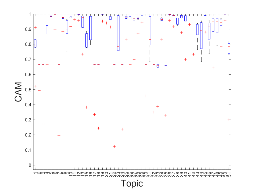
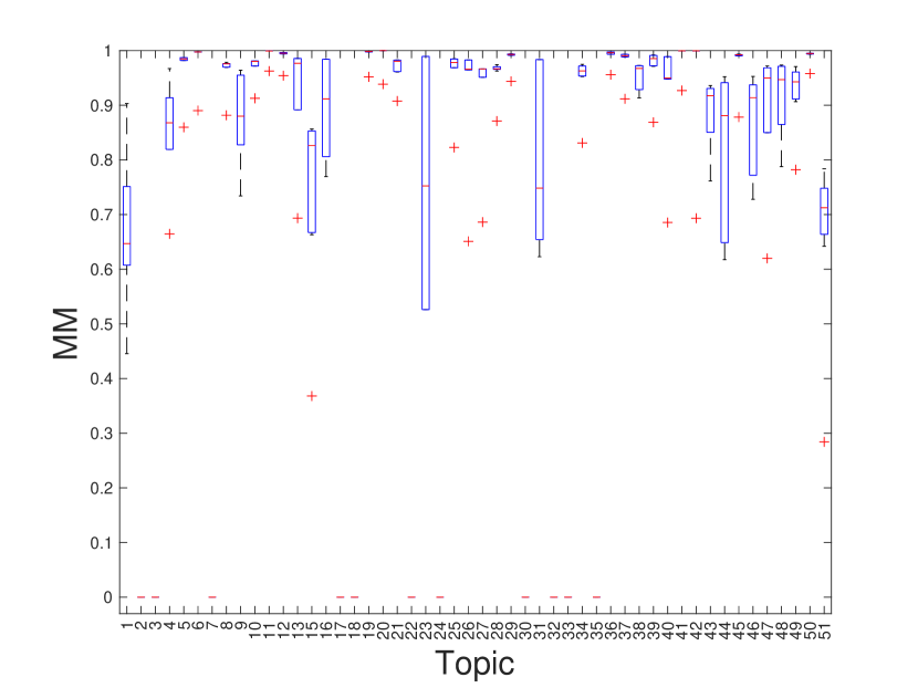
Figure 2. Box-plots for CAM and MM with NDCG on the Decision Track 2019. Topic numbers are on the $x$-axis and measures scores on the $y$-axis. The maximum value for CAM and MM is variable and depends on the topic and the aspects.

Problem 1: MM is ill-defined.

As the harmonic mean is not defined with zero values, MM is not defined if $\exists a\in A$ such that $\mu(\hat{r}_{t,a})=0$, e.g., a ranking does not retrieve any correct or relevant document. To compute MM even in these cases, as the denominator in Eq. (6) tends to $+\infty$ if any $\mu(\hat{r}_{t,a})$ tends to zero, we set $\text{MM}(r_{t})=0$. For classification measures, this problem is called the Strong Definiteness Axiom (Sebastiani, 2015). It represents a serious issue for collections where there are a few documents with a positive label for certain aspects. For example, for the Task Tracks, since useful documents are very sparse, many systems are not able to retrieve any useful document and they all have a $0$ score, independently of the number of relevant documents they retrieve. TOMA does not have this problem, because we first assign a weight to each tuple of labels and then compute a single-aspect evaluation measure $\mu$, thus there is no division by $0$ and TOMA is well defined.

Problem 2: CAM and MM can range in different intervals.

Given a set of documents $D$ and a set of aspects $A$, by definition CAM and MM are multi-aspect evaluation measures $M\colon D^{*}\to[0,X]$, where $D^{*}$ is the set of rankings and $X\leq 1$. Depending on $D$ and $A$, there exist cases with $X<1$.

To prove this claim, we need to show that when $M$ is CAM or MM, $\exists\ D,A$ such that:

(7) $$\max_{r\in D^{*}}M(\hat{r}_{t})<1$$

i.e., for each ranking of documents in $D^{*}$ the maximum measure score will be less than $1$. To build such an example, the set $D$ needs to contain documents with not comparable tuples of labels:

(8) $$\exists d_{1},d_{2}\in D\colon\textrm{GT}(d_{1})\not\sqsubseteq\textrm{GT}(d_{2})\textrm{ and }\textrm{GT}(d_{2})\not\sqsubseteq\textrm{GT}(d_{1})\iff\\ \exists d_{1},d_{2}\in D\textrm{ and }\exists a_{1},a_{2}\in A\colon\\ \textrm{GT}_{a_{1}}(d_{1})\prec_{a_{1}}\textrm{GT}_{a_{1}}(d_{2})\textrm{ and }\textrm{GT}_{a_{2}}(d_{2})\prec_{a_{2}}\textrm{GT}_{a_{2}}(d_{1})$$

In this case, CAM and MM cannot achieve a score equal to $1$ as illustrated by the following example.

Consider the example in $\S$3.4 with $A=\{$relevance, correctness$\}$. Let $D$ be a set with $3$ documents $D=\{d_{1},d_{2},d_{3}\}$ with labels $\textrm{GT}(d_{1})=(\texttt{mr},\texttt{c})$, $\textrm{GT}(d_{2})=(\texttt{hr},\texttt{pc})$ and $\textrm{GT}(d_{3})=(\texttt{hr},\texttt{nc})$. Documents $(d_{1},d_{2})$ and $(d_{1},d_{3})$ are not comparable and there is no unequivocal way of sorting them, e.g., it is not clear if $d_{1}$ should be ranked before $d_{2}$ or vice-versa.

Let us consider CAM and MM instantiated with AP and NDCG. For AP we use a harsh mapping for relevance and correctness, i.e., $\{\texttt{fr},\texttt{hr}\}\mapsto 1$ and $\{\texttt{mr},\texttt{nr}\}\mapsto 0$, and $\texttt{c}\mapsto 1$ and $\{\texttt{pc},\texttt{nc}\}\mapsto 0$. For NDCG we map each category to a different integer, for relevance we have: $\texttt{hr}\mapsto 15$, $\texttt{fr}\mapsto 10$, $\texttt{mr}\mapsto 5$, $\texttt{nr}\mapsto 0$, and for correctness we have: $\texttt{c}\mapsto 10$, $\texttt{pc}\mapsto 5$, $\texttt{nc}\mapsto 0$. The NDCG ideal ranking (Järvelin and Kekäläinen, 2002) for relevance is: $(\texttt{hr},\texttt{hr},\texttt{mr})$ and for correctness is $(\texttt{c},\texttt{pc},\texttt{nc})$. The NDCG $\log$ base is set to $2$.

For TOMA we use the embedding of the first row in Tab. 1 and as weight function we map each equivalence class to a different integer with step $1$. We instantiate TOMA with AP and NDCG with log base $2$ (Tab. 3). Since AP does not handle multi-graded weights, we map the top half of the equivalence classes to $1$ and the rest to $0$. Tab. 3 shows CAM, MM, and TOMA scores instantiated with AP NDCG for each possible ranking of documents in $D$.

In Tab. 3 none of the rankings in $D^{*}$ can achieve a score equal to $1$ for CAM and MM, while TOMA has at least one ranking with score $1$. In CAM and MM this happens because, any way we sort the documents, either we penalize correctness, e.g., $(d_{2},d_{3},d_{1})$ or we penalize relevance, e.g., $(d_{1},d_{2},d_{3})$. TOMA does not have this problem, since it first defines how to sort tuples of labels, then weights them accordingly and computes the measure score. Thus, if we sort documents in the order induced by $\preceq_{*}$, we obtain a score equal to $1$ (proof in the appendix). Experiments on real data confirm this, as detailed next.

Estimating CAM and MM Upper Bound

With the following experiment we show that with real data CAM and MM can be upper bounded by a value $X$ lower than $1$. To estimate the value $X$ with real data, we generate different ideal rankings of documents with different strategies. The intuition is that by ranking documents in the best possible way, we should achieve a score equal to $1$, as it happens for any single-aspect evaluation measure computed against the ideal ranking. Since CAM and MM do not define how to sort documents, i.e., a total order relation $\preceq_{*}$, we need to test different possible strategies to build these ideal rankings.

First, we define the ideal rankings obtained with a recursive strategy: these are the ideal rankings for each aspect when considered separately, e.g., for $3$ aspects, $a_{1}$, $a_{2}$ and $a_{3}$, with a preference order where $a_{1}$ is followed by $a_{2}$, followed by $a_{3}$: (1) we sort the documents with decreasing label for $a_{1}$; (2) among the documents with the same label for $a_{1}$, we sort the documents with decreasing label for $a_{2}$; (3) among the documents with the same label for $a_{1}$ and $a_{2}$, we sort the documents with decreasing label for $a_{3}$. We generate these ideal rankings for each possible preference order among the aspects.

We also generate $3$ additional ideal rankings: (1) we sum the weights across aspects and sort the documents by this sum; (2) we sum the squared weights across aspects and sort the documents by this sum; (3) we consider the highest weight across aspects and sort documents by their highest weight regardless of the aspect.

Fig. 2 reports the distributions of CAM with AP scores for the ideal rankings for the Decision Track 2019. These distributions depend on the aspect and the topic. We see that the upper bound $X$ is variable and depends on the topic: just for $2\%$ of topics it is equal to $1$ and for $26\%$ topics it is lower than $0.9$. We obtain similar or even more extreme distributions of scores for all the other tracks (except for Misinformation 2020, reported in the online appendix).

Interpretability of CAM and MM scores

Problem $2$ is especially important because it affects the interpretability of CAM and MM scores. When a measure is used to assess the quality of a single ranking in isolation, it should be intuitively interpretable (Kumar and Vassilvitskii, 2010), e.g., NDCG=$0.6$ has the intuitive interpretation that the ranking can be further improved by $0.4$. If TOMA is instantiated with NDCG, the intuitive interpretability of NDCG holds, but if CAM or MM are instantiated with NDCG, the intuitive interpretability of NDCG is lost: by the arguments above, CAM and MM may fail to obtain an optimal score of $1$, and the optimal score depends on $A$ and $D$, hence it cannot in general be known a priori.

This issue is important for MM, which is affected also by Problem $1$, and therefore may have $X<<1$. Thus MM scores can be compressed towards $0$, and this can lead to cases with many ties, where it is hard to distinguish between different rankings.

4.3. Experimental Findings

Table 4. Kendall’s $\tau$ correlation between rankings of systems and discriminative power (the higher, the better; best is in bold). Not all aspect combinations occur in all tracks (marked grey).

	WEB2009		WEB2010		WEB2011		WEB2012		WEB2013		WEB2014		TASK15		TASK16		DECISION19		MISINFO 2020
	NDCG	AP	NDCG	AP	NDCG	AP	NDCG	AP	NDCG	AP	NDCG	AP	NDCG	AP	NDCG	AP	NDCG	AP	NDCG	AP
	CORRELATION
EUCL - CAM	0.25	0.16	0.18	0.12	0.21	0.11	0.31	0.26	0.22	0.12	0.30	0.23	0.68	0.54	0.63	0.55	0.76	0.60	0.72	0.51
EUCL - MM	0.07	0.04	0.05	0.00	0.06	0.03	0.16	0.13	0.12	0.04	0.17	0.04	0.36	0.17	0.02	-0.10	0.46	0.31	0.45	0.27
MANH - CAM	0.22	0.16	0.21	0.12	0.16	0.11	0.34	0.26	0.31	0.12	0.41	0.23	0.62	0.54	0.60	0.55	0.69	0.60	0.72	0.51
MANH - MM	0.06	0.04	0.01	0.01	0.06	0.03	0.16	0.13	0.11	0.04	0.15	0.04	0.28	0.17	-0.06	-0.10	0.41	0.31	0.45	0.27
CHEB - CAM	0.01	0.02	0.06	0.05	0.02	0.02	0.19	0.15	0.11	0.00	0.19	0.07	0.26	0.16	-0.13	-0.18	0.27	0.27	0.29	0.24
CHEB - MM	0.06	0.09	0.00	0.03	0.09	0.01	0.19	0.16	0.12	0.08	0.14	0.05	0.88	0.86	0.52	0.53	0.58	0.60	0.54	0.52
EUCL - MANH	0.36	1.00	0.19	1.00	0.21	1.00	0.34	1.00	0.20	1.00	0.34	1.00	0.87	1.00	0.71	1.00	0.72	1.00	1.00	1.00
EUCL - CHEB	0.01	0.02	0.10	0.03	0.01	0.03	0.32	0.11	0.22	0.04	0.30	0.12	0.33	0.19	-0.21	-0.21	0.28	0.21	0.26	0.20
MANH - CHEB	0.01	0.02	0.03	0.03	0.02	0.03	0.21	0.11	0.10	0.04	0.18	0.12	0.32	0.19	-0.24	-0.21	0.25	0.21	0.26	0.20
CAM - MM	0.10	0.05	0.05	0.01	0.11	-0.01	0.23	0.13	0.16	0.03	0.26	0.04	0.30	0.18	0.09	0.00	0.51	0.41	0.51	0.42
	CORRELATION
Relevance - Popularity	0.03	0.05	0.01	0.0	0.01	0.02	0.09	0.09	0.06	0.01	0.07	0.02	0.04	0.04	-0.03	0.01
Relevance - Non-spam	0.05	0.03	0.02	0.0	0.03	0.01	0.07	0.05	-0.02	-0.01	0.07	-0.01	0.25	0.17	-0.07	-0.08
Popularity - Non-spam	0.04	0.03	0.02	-0.01	0.04	0.01	0.07	0.04	-0.03	-0.02	0.04	0.00	0.07	0.02	0.08	0.06
Relevance - Usefulness													0.75	0.75	0.75	0.74
Usefulness - Popularity													0.10	0.06	-0.04	0.00
Usefulness - Non-spam													0.40	0.33	-0.16	-0.19
Credibility - Correctness																	0.26	0.26	0.28	0.24
Relevance - Credibility																	0.33	0.33	0.29	0.25
Relevance - Correctness																	0.42	0.49	0.49	0.47
	DISCRIMINATIVE POWER OF MEASURES
CAM	75.98	64.43	66.32	61.23	75.14	61.64	68.71	56.74	76.89	57.05	85.06	78.85	53.33	33.33	72.22	55.56	72.58	70.56	71.53	70.90
MM	75.61	50.58	72.89	67.79	67.32	67.81	62.68	56.12	80.71	46.99	74.25	53.56	0.00	0.00	0.00	0.00	60.08	53.23	68.31	62.20
EUCL	75.29	72.64	62.96	66.75	75.14	70.33	66.13	64.10	75.14	59.45	80.92	78.85	66.67	66.67	69.44	75.00	73.59	73.99	72.86	75.14
MANH	76.66	72.68	63.59	67.14	77.32	70.38	66.05	64.18	76.67	59.34	86.44	79.08	66.67	53.33	75.00	75.00	73.79	73.79	73.02	74.98
CHEB	50.18	6.32	59.82	51.49	73.06	50.11	61.08	39.36	77.10	49.34	75.17	66.21	0.00	0.00	0.00	0.00	42.54	29.84	65.41	53.33

Empirically, evaluation measures are commonly assessed in terms of their correlation (Ferrante et al., 2019a), discriminative power (Sakai, 2007), informativeness (Aslam et al., 2005), intuitiveness (Sakai, 2012), and unanimity (Albahem et al., 2019). Out of these, we report only correlation and discriminative power because the rest does not apply: the informativeness test (Aslam et al., 2005) requires a precision recall-curve, which cannot be defined for multi-aspect evaluation; the intuitiveness test (Sakai, 2012) requires simple single-aspect measures (e.g. precision, recall), which do not apply to multi-aspect evaluation; the unanimity test (Albahem et al., 2019), which is defined for multi-aspect evaluation, requires that all the simple measures agree over all aspects, which happened extremely rarely in our data, especially as the number of aspects increased (see the low correlation among aspects in Tab. 4).

4.3.1. Correlation Analysis

We use Kendall’s $\tau$ (Kendall, 1945) to estimate TOMA’s correlation to MM and CAM. Generally, if a new evaluation measure strongly correlates to an existing one, it is likely to represent redundant information (Webber et al., 2008). We use Kendall’s $\tau$ because it has better gross-error sensitivity than the Pearson correlation coefficient (Croux and Dehon, 2010), and because the Spearman correlation coefficient cannot handle ties. As per (Ferrante et al., 2019a), we compute the correlation topic-by-topic. For each topic we consider the Rankings of Submitted runs (RoS) corresponding to two different measures (one ranking per measure) and then compute Kendall’s $\tau$ between the two RoS. We report Kendall’s $\tau$ averaged across all topics. As per (Voorhees, 1998, 2001), we consider two rankings equivalent if Kendall’s $\tau$ is greater than $0.9$.

Tab. 4 shows the findings, which are summarised as follows:

• The RoS corresponding to EUCL - MANH are equivalent ($\tau=1$) at all times for AP. This perfect correlation for AP happens because, by definition, when the sets of equivalence classes from these approaches are mapped to binary labels, they produce the exact same set of labels (see also Tab. 3). For NDCG, $\tau=0.19-1$, where higher correlations correspond to tracks where some aspects are not assessed for non relevant documents, thus there are less extreme cases and EUCL is more similar to MANH.

• The RoS corresponding to (EUCL, MANH) - CHEB are very weakly correlated ($\tau=0.01-0.32$), this is due to Chebyshev distance being very harsh, since many equivalence classes are considered equivalent to the class of non relevant documents.

• The RoS corresponding to EUCL - CAM and MANH - CAM are very weakly correlated ($\tau=0.11-0.41$) for the Web tracks, but moderately correlated ($\tau=0.54-0.76$) for the Task, Decision and Misinformation tracks. This happens because: (i) the runs submitted to the Web tracks were not designed to account for multiple aspects and (ii) for the Task, Decision and Misinformation tracks, usefulness, credibility and correctness are not assessed for non relevant documents. Therefore, since some of the values are missing, these methods generate a lower number of equivalence classes, which make them more similar to CAM. Whereas, for the Web tracks, popularity and non-spamminess are approximated for all documents, meaning that MANH and EUCL can possibly generate all the different equivalence classes, even for non relevant documents. This makes them less similar to CAM than on the Task or Decision tracks.

• For the Task, Decision and Misinformation tracks, the RoS corresponding to MM and CHEB are moderately correlated ($\tau=0.52-0.88$). The fact that, for these tracks, usefulness, credibility and correctness are not assessed for non relevant documents, means that all the documents that are mapped to a $0$ weight with CHEB, are also contributing as $0$ to MM.

To contextualise these findings, the middle part of Tab. 4 shows the $\tau$ values of the RoS corresponding to evaluating a single aspect only. Overall, the resulting correlations are low to non-existent, meaning that considering multiple aspects affects the final evaluation outcome. The two exceptions where the correlation between RoS is not very low are:

• For Task 2015-2016, for relevance - usefulness, $\tau=0.74-0.75$. This happens because: (1) usefulness is not assessed for non relevant documents, thus non relevant documents are assumed to be not useful, and (2) usefulness is a very sparse signal (1.75% of documents are useful).

• For the Decision and Misinformation Tracks, for all aspects, $\tau=0.24-0.49$. Again here credibility and correctness are not assessed for non relevant documents ($6.89\%$ of documents are credible and $9.75\%$ are correct for the Decision Track; $13.73\%$ of documents are correct and $27.62\%$ are credible for the Misinformation Track), so the correlation is not as high as for the Task tracks.

Overall, the most correlated RoS correspond to: EUCL - MANH ($\tau$ up to $1$), (EUCL, MANH)- CAM ($\tau$ up to $0.76$), and CHEB - MM ($\tau$ up to $0.88$). Intuitively, EUCL and MANH may be more similar to CAM (mean), while CHEB may be more similar to MM (harmonic mean). Thus TOMA proposes an alternative evaluation framework, which overcomes CAM and MM anomalies (see $\S$4.2). The fact that $\tau$ values between TOMA and the baselines are never above $0.9$ means that there are noticeable differences between the RoS generated by TOMA and by CAM or MM. Recall that all measures are instantiated with NDCG or AP, meaning that differences between them are due to how multi-aspect labels are treated.

4.3.2. Discriminative Power

We use Bootstrap Hypothesis Test (Sakai, 2007) to estimate the discriminative power of TOMA, CAM and MM. Given a set of topics and a set of runs, we first generate subsets of topics by sampling with replacement the complete set of topics. We set the number of bootstrap samples to $10\,000$. To assess whether the measure scores for pairs of runs can be considered different at a given confidence level, we use a Paired Bootstrap Hypothesis Test. The confidence level is $1-\alpha$, where $\alpha$ is the Type I Error, i.e., the probability to consider two systems different even if they are equivalent. We set $\alpha=0.01$, requiring strong evidence for two systems to be different.

Tab. 4 (bottom part) displays the results of the discriminative power analysis, where the higher the score, the more discriminative (i.e., the better) the approach. We see that $16/20$ times either MANH ($12/20$) or EUCL ($6/20$) is best. The remaining $4$ times, MM is best $3$ times, and CAM once. We also see that CHEB is never best, and for Task 2015-2016 it is actually zero. This is due to the very small amount of positive labels for usefulness in that track. For the same reason, MM is also zero for the same track. Overall, CHEB is the least discriminative measure, followed by MM; this is due to how these methods treat tuples of labels: the fact that if one aspect label is zero, then the whole score is zero, practically means that many runs are considered equal purely on that basis.

4.3.3. Zero-aspect documents

Table 5. Number of times (%) that the labels of all aspects sum to $0$ for a document that is ranked at position $1$-$5$ (column 1) in a run that has been assessed as best per $\{$topic, track, year$\}$ separately with $\{$CAM, MM, EUCL, MANH, CHEB$\}$ using a retrieval cutoff of 5. The lower, the better.

Rank	CAM	MM	EUCL	MANH	CHEB
1	51 (1.18%)	131 (3.02%)	39 (0.90%)	33 (0.76%)	154 (3.55%)
2	65 (1.50%)	159 (3.67%)	50 (1.15%)	48 (1.11%)	179 (4.13%)
3	103 (2.38%)	202 (4.66%)	88 (2.03%)	78 (1.80%)	185 (4.17%)
4	102 (2.35%)	173 (3.99%)	86 (1.99%)	74 (1.71%)	183 (4.23%)
5	107 (2.47%)	196 (4.53%)	95 (2.19%)	81 (1.87%)	205 (4.73%)
1-5	428 (9.88%)	861 (19.88%)	358 (8.27%)	314 (7.25%)	906 (20.92%)

Our next analysis is motivated by the empirical trash$@k$ measure often used in industry to mitigate the high cost of retrieving “trash” in high ranks. We count how often the labels of all aspects sum to zero for a document that has been ranked at position $1$-$5$ in a run that has been assessed as the best run per track year, on a per query basis, using a retrieval cutoff of $5$, separately with $\{$CAM, MM, EUCL, MANH, CHEB$\}$ when instantiated separately with NDCG and AP. When the labels of all aspects sum to zero, this means that the corresponding document is of the worst quality. Ideally, such documents should not be retrieved, but when they do, they should not be in the top 5.

In Tab. 5 we see that MANH is associated with the lowest amount of zero-aspect documents, closely followed by EUCL. This happens because MANH is designed so that the higher the sum of a document’s labels across aspects, the better that document will be deemed. CHEB is overall worst, closely followed by MM. This closeness between EUCL-MANH and CHEB-MM agrees with the previous correlation and discriminative power analysis. Overall, MANH (and less so EUCL) penalise low quality documents the best.

4.3.4. Document quality @1-100

Table 6. Average sum of aspect labels for a document that is ranked at position $1$-$100$ (column 1) in a run that has been assessed as best per $\{$topic, track, year$\}$ separately with $\{$CAM, MM, EUCL, MANH, CHEB$\}$ using a retrieval cutoff of 100. The higher, the better.

Ranks	CAM	MM	EUCL	MANH	CHEB
1-25	1.70	1.49	1.67	1.69	1.39
26-50	0.85	0.78	0.91	0.94	0.70
51-75	0.57	0.53	0.63	0.64	0.48
76-100	0.40	0.39	0.43	0.44	0.36

We look at the quality of documents that have been ranked at positions 1-100 in a run that has been assessed as best per $\{$topic, track, year$\}$ separately with $\{$CAM, MM, EUCL, MANH, CHEB$\}$, when instantiated separately with NDCG and AP, using a retrieval cutoff of $100$. We split the ranks $1$-$100$ into four sets ($1$-$25$, $26$-$50$, $51$-$75$, $76$-$100$). For each document in each set, we sum the labels of its aspects, and we report the average of these sums, which can be seen as an approximation of the average document quality (the higher, the better).

As expected, we see that the numbers in Tab. 6, and hence document quality, drop as we move down the ranking, at all times. Comparing across columns however, we see that, for the runs that were assessed as best by MANH, document quality is overall, albeit marginally, the best, at ranks 26-100. This illustrates that the design of MANH (the higher the sum of a document’s labels across aspects, the better that document will be considered) gives it the practical advantage of, not only reducing the amount of low quality documents in the top ranks (as seen in Tab. 5), but also of increasing the quality of documents further down the ranking, as we see now. Again, as previously, we observe that EUCL is a close second-best method, CHEB and MM are overall worst, and CAM is in between (although best, together with MANH, for the top ranks).

5. Conclusion and Limitations

Multi-aspect evaluation is a special case of IR evaluation where the ranked list of documents returned by an IR system in response to a query must be assessed in terms of not only relevance, but also other aspects (or dimensions) of the ranked documents, e.g., credibility or usefulness. We presented a principled multi-aspect evaluation approach, called TOMA, that is defined for any number and type of aspect, and that allows for (i) aspects having different gradings, (ii) any relative importance weighting for different aspects, and (iii) integration with any existing single-aspect evaluation measure, such as NDCG. We showed that TOMA has better discriminative power than prior approaches to multi-aspect evaluation, and that it is better at rewarding high quality documents across the ranking.

One limitation of TOMA is represented by the arbitrary choices of the embedding function, the distance function and the weight function. The embedding function maps labels from a nominal or ordinal scale to an interval or ratio scale. This calls for a in-depth investigation of the theoretical properties of TOMA using the existing axiomatic treatments of IR effectiveness measures (Amigó et al., 2018a; Maddalena and Mizzaro, 2014; Busin and Mizzaro, 2013; Amigó and Mizzaro, 2020; Ferrante et al., 2021). This also motivates a deep analysis of the interactions between different aspects and/or documents and how to handle them with TOMA, for example by defining a proper embedding and distance function which account for aspects as diversity, novelty, and redundancy. Moreover, the embedding function combined with the distance function can generate a large number of tuples of labels, which can be mapped to different integers through the weight function. This might be a problem for gain based measures, thus a possible solution is to use TOMA to define the ideal ranking and then use effectiveness measures based on similarity to ideal rankings  (Clarke et al., 2020c, b, 2021). Finally, the empirical impact of varying both distance and weight functions should also be investigated, as should the impact of employing further multi-graded measures as ERR (Chapelle et al., 2009), and the alignment of our current approach with real user preferences.

Acknowledgments. This paper is partially supported by the EU Horizon 2020 research and innovation programme under the MSCA grant No. 893667.

References

- (1)
- Agrawal et al. (2009) R. Agrawal, S. Gollapudi, A. Halverson, and S. Ieong. 2009. Diversifying Search Results. In Proc. 2nd ACM International Conference on Web Searching and Data Mining (WSDM 2009), R. Baeza-Yates, P. Boldi, B. Ribeiro-Neto, and B. B. Cambazoglu (Eds.). ACM Press, New York, USA, 5–14.
- Albahem et al. (2019) A. Albahem, , D. Spina, F. Scholer, and L. Cavedon. 2019. Meta-evaluation of Dynamic Search: How Do Metrics Capture Topical Relevance, Diversity and User Effort?. In Advances in Information Retrieval. Proc. 41st European Conference on IR Research (ECIR 2019), L. Azzopardi, B. Stein, N. Fuhr, P. Mayr, C. Hauff, and D. Hiemstra (Eds.). Lecture Notes in Computer Science (LNCS) 10772, Springer, Heidelberg, Germany, 607–620.
- Amigó et al. (2018a) E. Amigó, F. Giner, S. Mizzaro, and D. Spina. 2018a. A Formal Account of Effectiveness Evaluation and Ranking Fusion. In Proc. 4th ACM SIGIR International Conference on the Theory of Information Retrieval (ICTIR 2018), D. Song, T.-Y. Liu, L. Sun, P. Bruza, M. Melucci, F. Sebastiani, and G. Hui Yang (Eds.). ACM Press, New York, USA, 123–130.
- Amigó and Mizzaro (2020) E. Amigó and S. Mizzaro. 2020. On the Nature of Information Access Evaluation Metrics: a Unifying Framework. Information Retrieval Journal 23, 3 (2020), 318–386. https://doi.org/10.1007/s10791-020-09374-0
- Amigó et al. (2018b) E. Amigó, D. Spina, and J. Carrillo-de Albornoz. 2018b. An Axiomatic Analysis of Diversity Evaluation Metrics: Introducing the Rank-Biased Utility Metric. In Proc. 41th Annual International ACM SIGIR Conference on Research and Development in Information Retrieval (SIGIR 2018), K. Collins-Thompson, Q. Mei, B. Davison, Y. Liu, and E. Yilmaz (Eds.). ACM Press, New York, USA, 625–634.
- Aslam et al. (2005) J. A. Aslam, E. Yilmaz, and V. Pavlu. 2005. The maximum entropy method for analyzing retrieval measures. In SIGIR 2005: Proceedings of the 28th Annual International ACM SIGIR Conference on Research and Development in Information Retrieval, Salvador, Brazil, August 15-19, 2005, Ricardo A. Baeza-Yates, Nivio Ziviani, Gary Marchionini, Alistair Moffat, and John Tait (Eds.). ACM, 27–34. https://doi.org/10.1145/1076034.1076042
- Buckley and Voorhees (2005) C. Buckley and E. M. Voorhees. 2005. Retrieval System Evaluation. In TREC. Experiment and Evaluation in Information Retrieval, D. K. Harman and E. M. Voorhees (Eds.). MIT Press, Cambridge (MA), USA, 53–78.
- Burges et al. (2005) C. Burges, T. Shaked, E. Renshaw, A. Lazier, M. Deeds, N. Hamilton, and G. Hullender. 2005. Learning to Rank using Gradient Descent. In Proc. 22nd International Conference on Machine Learning (ICML 2005), S. Dzeroski, L. De Raedt, and S. Wrobel (Eds.). ACM Press, New York, USA, 89–96.
- Busin and Mizzaro (2013) L. Busin and S. Mizzaro. 2013. Axiometrics: An Axiomatic Approach to Information Retrieval Effectiveness Metrics. In Proc. 4th International Conference on the Theory of Information Retrieval (ICTIR 2013), O. Kurland, D. Metzler, C. Lioma, B. Larsen, and P. Ingwersen (Eds.). ACM Press, New York, USA, 22–29.
- Chapelle et al. (2009) O. Chapelle, D. Metzler, Y. Zhang, and P. Grinspan. 2009. Expected Reciprocal Rank for Graded Relevance. In Proc. 18th International Conference on Information and Knowledge Management (CIKM 2009), D. W.-L. Cheung, I.-Y. Song, W. W. Chu, X. Hu, and J. J. Lin (Eds.). ACM Press, New York, USA, 621–630.
- Clarke et al. (2009) C. Clarke, N. Craswell, and I. Soboroff. 2009. Overview of the TREC 2009 Web Track. In TREC. National Institute of Standards and Technology (NIST).
- Clarke et al. (2020a) Charles Clarke, Maria Maistro, Mark Smucker, and Guido Zuccon. 2020a. Overview of the TREC 2020 Health Misinformation Track (to appear). In Proceedings of the Twenty-Nine Text REtrieval Conference, TREC 2020, Gaithersburg, Maryland, USA, November 16-19, 2020 (NIST Special Publication), Ellen M. Voorhees and Angela Ellis (Eds.), Vol. -. National Institute of Standards and Technology (NIST).
- Clarke and Cormack (2011) C. L. A. Clarke and G. V. Cormack. 2011. Overview of the TREC 2010 Web Track. In TREC. National Institute of Standards and Technology (NIST).
- Clarke et al. (2011) C. L. A. Clarke, N. Craswell, I. Soboroff, and E. M. Voorhees. 2011. Overview of the TREC 2011 Web Track. In TREC. National Institute of Standards and Technology (NIST).
- Clarke et al. (2012) C. L. A. Clarke, N. Craswell, and E. M. Voorhees. 2012. Overview of the TREC 2012 Web Track. In TREC. National Institute of Standards and Technology (NIST).
- Clarke et al. (2008) C. L. A. Clarke, M. Kolla, G. V. Cormack, O. Vechtomova, A. Ashkan, S. Büttcher, and I. MacKinnon. 2008. Novelty and Diversity in Information Retrieval Evaluation. In Proc. 31st Annual International ACM SIGIR Conference on Research and Development in Information Retrieval (SIGIR 2008), T.-S. Chua, M.-K. Leong, D. W. Oard, and F. Sebastiani (Eds.). ACM Press, New York, USA, 659–666.
- Clarke et al. (2020b) Charles L. A. Clarke, Mark D. Smucker, and Alexandra Vtyurina. 2020b. Offline Evaluation by Maximum Similarity to an Ideal Ranking. In CIKM ’20: The 29th ACM International Conference on Information and Knowledge Management, Virtual Event, Ireland, October 19-23, 2020, Mathieu d’Aquin, Stefan Dietze, Claudia Hauff, Edward Curry, and Philippe Cudré-Mauroux (Eds.). ACM, 225–234.
- Clarke et al. (2020c) Charles L. A. Clarke, Alexandra Vtyurina, and Mark D. Smucker. 2020c. Offline Evaluation without Gain. In ICTIR ’20: The 2020 ACM SIGIR International Conference on the Theory of Information Retrieval, Virtual Event, Norway, September 14-17, 2020, Krisztian Balog, Vinay Setty, Christina Lioma, Yiqun Liu, Min Zhang, and Klaus Berberich (Eds.). ACM, 185–192.
- Clarke et al. (2021) C. L. A. Clarke, A. Vtyurina, and M. D. Smucker. 2021. Assessing Top- Preferences. arXiv:cs.IR/2007.11682
- Collins-Thompson et al. (2014) K. Collins-Thompson, P. Bennett, F. Diaz, C. L. A. Clarke, and E. M. Voorhees. 2014. TREC 2014 Web Track Overview. In The Twenty-Second Text REtrieval Conference Proceedings (TREC 2013), E. M. Voorhees (Ed.). National Institute of Standards and Technology (NIST), Special Publication 500-302, Washington, USA.
- Collins-Thompson et al. (2015) K. Collins-Thompson, P. Bennett, F. Diaz, C. L. A. Clarke, and E. M. Voorhees. 2015. TREC 2014 Web Track Overview. In The Twenty-Third Text REtrieval Conference Proceedings (TREC 2014), E. M. Voorhees and A. Ellis (Eds.). National Institute of Standards and Technology (NIST), Special Publication 500-308, Washington, USA.
- Croux and Dehon (2010) C. Croux and C. Dehon. 2010. Influence Functions of the Spearman and Kendall Correlation Measures. Statistical Methods & Applications 19 (2010), 497–515. https://doi.org/10.1007/s10260-010-0142-z
- Ferrante et al. (2021) M. Ferrante, N. Ferro, and N Fuhr. 2021. Towards Meaningful Statements in IR Evaluation. Mapping Evaluation Measures to Interval Scales. CoRR abs/2101.02668 (2021). arXiv:2101.02668 https://arxiv.org/abs/2101.02668
- Ferrante et al. (2019a) M. Ferrante, N. Ferro, and E. Losiouk. 2019a. How do Interval Scales Help us with Better Understanding IR Evaluation Measures? Information Retrieval Journal (2019). https://doi.org/10.1007/s10791-019-09362-z
- Ferrante et al. (2015) M. Ferrante, N. Ferro, and M. Maistro. 2015. Towards a Formal Framework for Utility-Oriented Measurements of Retrieval Effectiveness. In Proceedings of the 2015 International Conference on The Theory of Information Retrieval (ICTIR ’15). Association for Computing Machinery, New York, NY, USA, 21–30. https://doi.org/10.1145/2808194.2809452
- Ferrante et al. (2017) M. Ferrante, N. Ferro, and Silvia P. 2017. Are IR Evaluation Measures on an Interval Scale?. In Proceedings of the ACM SIGIR International Conference on Theory of Information Retrieval (ICTIR ’17). Association for Computing Machinery, New York, NY, USA, 67–74. https://doi.org/10.1145/3121050.3121058
- Ferrante et al. (2019b) M. Ferrante, N. Ferro, and S. Pontarollo. 2019b. A General Theory of IR Evaluation Measures. IEEE Transactions on Knowledge and Data Engineering (TKDE) 31, 3 (2019), 409–422.
- Halmos (1974) P. R. Halmos. 1974. Naive Set Theory. Springer-Verlag, New York, USA.
- Järvelin and Kekäläinen (2002) K. Järvelin and J. Kekäläinen. 2002. Cumulated Gain-Based Evaluation of IR Techniques. ACM Trans. Inf. Syst. 20, 4 (Oct. 2002), 422–446. https://doi.org/10.1145/582415.582418
- Kazai et al. (2004) G. Kazai, S. Masood, and M. Lalmas. 2004. A Study of the Assessment of Relevance for the INEX’02 Test Collection. In Advances in Information Retrieval. Proc. 26th European Conference on IR Research (ECIR 2004), S. McDonald and J. Tait (Eds.). Lecture Notes in Computer Science (LNCS) 2997, Springer, Heidelberg, Germany, 296–310.
- Kekäläinen and Järvelin (2002) J. Kekäläinen and K. Järvelin. 2002. Using Graded Relevance Assessments in IR Evaluation. Journal of the American Society for Information Science and Technology (JASIST) 53, 13 (November 2002), 1120—1129.
- Kendall (1945) M. G. Kendall. 1945. The Treatment of Ties in Ranking Problems. Biometrika 33, 3 (November 1945), 239–251.
- Kumar and Vassilvitskii (2010) Ravi Kumar and Sergei Vassilvitskii. 2010. Generalized distances between rankings. In Proceedings of the 19th International Conference on World Wide Web, WWW 2010, Raleigh, North Carolina, USA, April 26-30, 2010, Michael Rappa, Paul Jones, Juliana Freire, and Soumen Chakrabarti (Eds.). ACM, 571–580. https://doi.org/10.1145/1772690.1772749
- Lioma et al. (2019) C. Lioma, M. Maistro, M. D. Smucker, , and D. Zuccon. 2019. Overview of the TREC 2019 Decision Track. In The Twenty-Eighth Text REtrieval Conference Proceedings (TREC 2019), E. M. Voorhees and A. Ellis (Eds.). National Institute of Standards and Technology (NIST), Special Publication 500-331, Washington, USA.
- Lioma et al. (2017) C. Lioma, J. G. Simonsen, and B. Larsen. 2017. Evaluation Measures for Relevance and Credibility in Ranked Lists. In Proc. 3rd ACM SIGIR International Conference on the Theory of Information Retrieval (ICTIR 2017), J. Kamps, E. Kanoulas, M. de Rijke, H. Fang, and E. Yilmaz (Eds.). ACM Press, New York, USA, 91–98.
- Maddalena and Mizzaro (2014) E. Maddalena and S. Mizzaro. 2014. Axiometrics: Axioms of Information Retrieval Effectiveness Metrics. In Proc. 6th International Workshop on Evaluating Information Access (EVIA 2014), S. Mizzaro and R. Song (Eds.). National Institute of Informatics, Tokyo, Japan, 17–24.
- Palotti et al. (2018) J. Palotti, G. Zuccon, and A. Hanbury. 2018. MM: A New Framework for Multidimensional Evaluation of Search Engines. In Proc. 27th International Conference on Information and Knowledge Management (CIKM 2018), A. Cuzzocrea, J. Allan, N. W. Paton, D. Srivastava, R. Agrawal, A. Broder, M. J. Zaki, S. Candan, A. Labrinidis, A. Schuster, and H. Wang (Eds.). ACM Press, New York, USA, 1699–1702.
- Petersen et al. (2015) C. Petersen, C. Lioma, J. G. Simonsen, and B. Larsen. 2015. Entropy and Graph Based Modelling of Document Coherence Using Discourse Entities: An Application to IR. In Proceedings of the 2015 International Conference on The Theory of Information Retrieval (ICTIR ’15). ACM, New York, NY, USA, 191–200. https://doi.org/10.1145/2808194.2809458
- Sakai (2007) T. Sakai. 2007. Evaluating Information Retrieval Metrics Based on Bootstrap Hypothesis Tests. IPSJ Digital Courier 3 (2007), 625–642. https://doi.org/10.2197/ipsjdc.3.625
- Sakai (2012) T. Sakai. 2012. Evaluation with Informational and Navigational Intents. In Proc. 21st International Conference on World Wide Web (WWW 2012), A. Mille, F. L. Gandon, J. Misselis, M. Rabinovich, and S. Staab (Eds.). ACM Press, New York, USA, 499–508.
- Sebastiani (2015) F. Sebastiani. 2015. An Axiomatically Derived Measure for the Evaluation of Classification Algorithms. In Proc. 1st ACM SIGIR International Conference on the Theory of Information Retrieval (ICTIR 2015), J. Allan, W. B. Croft, A. P. de Vries, C. Zhai, N. Fuhr, and Y. Zhang (Eds.). ACM Press, New York, USA, 11–20.
- Tang and Yang (2017) Z. Tang and G. H. Yang. 2017. Investigating per Topic Upper Bound for Session Search Evaluation. In Proceedings of the ACM SIGIR International Conference on Theory of Information Retrieval (ICTIR ’17). Association for Computing Machinery, New York, NY, USA, 185–192. https://doi.org/10.1145/3121050.3121069
- Voorhees (1998) E. M. Voorhees. 1998. Variations in relevance judgments and the measurement of retrieval effectiveness. In Proc. 21st Annual International ACM SIGIR Conference on Research and Development in Information Retrieval (SIGIR 1998), W. B. Croft, A. Moffat, C. J. van Rijsbergen, R. Wilkinson, and J. Zobel (Eds.). ACM Press, New York, USA, 315–323.
- Voorhees (2001) E. M. Voorhees. 2001. Evaluation by Highly Relevant Documents. In Proc. 24th Annual International ACM SIGIR Conference on Research and Development in Information Retrieval (SIGIR 2001), D. H. Kraft, W. B. Croft, D. J. Harper, and J. Zobel (Eds.). ACM Press, New York, USA, 74–82.
- Voorhees and Ellis (2016) E. M. Voorhees and A. Ellis (Eds.). 2016. Proceedings of The Twenty-Fifth Text REtrieval Conference, TREC 2016, Gaithersburg, Maryland, USA, November 15-18, 2016. Vol. Special Publication 500-321. National Institute of Standards and Technology (NIST). http://trec.nist.gov/pubs/trec25/trec2016.html
- Webber et al. (2008) W. Webber, A. Moffat, J. Zobel, and T. Sakai. 2008. Precision-at-ten Considered Redundant. In Proceedings of the 31st Annual International ACM SIGIR Conference on Research and Development in Information Retrieval (SIGIR ’08). ACM, New York, NY, USA, 695–696. https://doi.org/10.1145/1390334.1390456
- Yao (1995) Y. Y. Yao. 1995. Measuring Retrieval Effectiveness Based on User Preference of Documents. Journal of the American Society for Information Science (JASIS) 46, 2 (1995), 133–145. https://doi.org/10.1002/(SICI)1097-4571(199503)46:2<133::AID-ASI6>3.0.CO;2-Z
- Yilmaz et al. (2016) E. Yilmaz, M. Verma, R. Mehrotra, E. Kanoulas, B. Carterette, and N. Craswell. 2016. Overview of the TREC 2015 Tasks Track. In The Twenty-Fourth Text REtrieval Conference Proceedings (TREC 2015), E. M. Voorhees and A. Ellis (Eds.). National Institute of Standards and Technology (NIST), Special Publication 500-319, Washington, USA.
- Zuccon (2016) G. Zuccon. 2016. Understandability Biased Evaluation for Information Retrieval. In Advances in Information Retrieval. Proc. 38th European Conference on IR Research (ECIR 2016), N. Ferro, F. Crestani, M.-F. Moens, J. Mothe, F. Silvestri, G. M. Di Nunzio, C. Hauff, and G. Silvello (Eds.). Lecture Notes in Computer Science (LNCS) 9626, Springer, Heidelberg, Germany, 280–292.