Zero-Shot Image Restoration Using
Denoising Diffusion Null-Space Model

Abstract

Most existing Image Restoration (IR) models are task-specific, which can not be generalized to different degradation operators. In this work, we propose the Denoising Diffusion Null-Space Model (DDNM), a novel zero-shot framework for arbitrary linear IR problems, including but not limited to image super-resolution, colorization, inpainting, compressed sensing, and deblurring. DDNM only needs a pre-trained off-the-shelf diffusion model as the generative prior, without any extra training or network modifications. By refining only the null-space contents during the reverse diffusion process, we can yield diverse results satisfying both data consistency and realness. We further propose an enhanced and robust version, dubbed DDNM⁺, to support noisy restoration and improve restoration quality for hard tasks. Our experiments on several IR tasks reveal that DDNM outperforms other state-of-the-art zero-shot IR methods. We also demonstrate that DDNM⁺ can solve complex real-world applications, e.g., old photo restoration.

1 Introduction

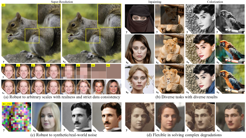
Figure 1: We use DDNM⁺ to solve various image restoration tasks in a zero-shot way. Here we show some of the results that best characterize our method, where $\mathbf{y}$ is the input degraded image and $\mathbf{x}_{0}$ represents the restoration result. Part (a) shows the results of DDNM⁺ on image super-resolution (SR) from scale 2$\times$ to extreme scale 256$\times$. Note that DDNM⁺ assures strict data consistency. Part (b) shows multiple results of DDNM⁺ on inpainting and colorization. Part (c) shows the results of DDNM⁺ on SR with synthetic noise and colorization with real-world noise. Part (d) shows the results of DDNM⁺ on old photo restoration. All the results here are yielded in a zero-shot way.

Image Restoration (IR) is a long-standing problem due to its extensive application value and its ill-posed nature (Richardson, 1972; Andrews & Hunt, 1977). IR aims at yielding a high-quality image $\hat{\mathbf{x}}$ from a degraded observation $\mathbf{y}=\mathbf{A}\mathbf{x}+\mathbf{n}$, where $\mathbf{x}$ stands for the original image and $\mathbf{n}$ represents a non-linear noise. $\mathbf{A}$ is a known linear operator, which may be a bicubic downsampler in image super-resolution, a sampling matrix in compressed sensing, or even a composite type. Traditional IR methods are typically model-based, whose solution can be usually formulated as:

$$\hat{\mathbf{x}}=\underset{\mathbf{x}}{\operatorname{arg\,min}} \frac{1}{2\sigma^{2}}||\mathbf{A}\mathbf{x}-\mathbf{y}||_{2}^{2}+\lambda\mathcal{R}(\mathbf{x}).$$ (1)

The first data-fidelity term $\frac{1}{2\sigma^{2}}||\mathbf{A}\mathbf{x}-\mathbf{y}||_{2}^{2}$ optimizes the result toward data consistency while the second image-prior term $\lambda\mathcal{R}(\mathbf{x})$ regularizes the result with formulaic prior knowledge on natural image distribution, e.g., sparsity and Tikhonov regularization. Though the hand-designed prior knowledge may prevent some artifacts, they often fail to bring realistic details.

The prevailing of deep neural networks (DNN) brings new patterns of solving IR tasks (Dong et al., 2015), which typically train an end-to-end DNN $\mathcal{D}_{\mathbf{\bm{\theta}}}$ by optimizing network parameters $\bm{\theta}$ following

$$\underset{\bm{\theta}}{\operatorname{arg\,min}} \sum_{i=1}^{N}||\mathcal{D}_{\bm{\theta}}(\mathbf{y}_{i})-\mathbf{x}_{i}||_{2}^{2},$$ (2)

where $N$ pairs of degraded image $\mathbf{y}_{i}$ and ground truth image $\mathbf{x}_{i}$ are needed to learn the mapping from $\mathbf{y}$ to $\mathbf{x}$ directly. Although end-to-end learning-based IR methods avoid explicitly modeling the degradation $\mathbf{A}$ and the prior term in Eq. 1 and are fast during inference, they usually lack interpretation. Some efforts have been made in exploring interpretable DNN structures (Zhang & Ghanem, 2018; Zhang et al., 2020), however, they still yield poor performance when facing domain shift since Eq. 2 essentially encourage learning the mapping from $\mathbf{y}_{i}$ to $\mathbf{x}_{i}$. For the same reason, the end-to-end learning-based IR methods usually need to train a dedicated DNN for each specific task, lacking generalizability and flexibility in solving diverse IR tasks. The evolution of generative models (Goodfellow et al., 2014; Bahat & Michaeli, 2014; Van Den Oord et al., 2017; Karras et al., 2019; 2020; 2021) further pushes the end-to-end learning-based IR methods toward unprecedented performance in yielding realistic results (Yang et al., 2021; Wang et al., 2021; Chan et al., 2021; Wang et al., 2022b). At the same time, some methods (Menon et al., 2020; Pan et al., 2021) start to leverage the latent space of pretrained generative models to solve IR problems in a zero-shot way. Typically, they optimize the following objective:

$$\underset{\mathbf{w}}{\operatorname{arg\,min}} \frac{1}{2\sigma^{2}}||\mathbf{A}\mathcal{G}(\mathbf{w})-\mathbf{y}||_{2}^{2}+\lambda\mathcal{R}(\mathbf{w}),$$ (3)

where $\mathcal{G}$ is the pretrained generative model, $\mathbf{w}$ is the latent code, $\mathcal{G}(\mathbf{w})$ is the corresponding generative result and $\mathcal{R}(\mathbf{w})$ constrains $\mathbf{w}$ to its original distribution space, e.g., a Gaussian distribution. However, this type of method often struggles to balance realness and data consistency.

The Range-Null space decomposition (Schwab et al., 2019; Wang et al., 2022a) offers a new perspective on the relationship between realness and data consistency: the data consistency is only related to the range-space contents, which can be analytically calculated. Hence the data term can be strictly guaranteed, and the key problem is to find proper null-space contents that make the result satisfying realness. We notice that the emerging diffusion models (Ho et al., 2020; Dhariwal & Nichol, 2021) are ideal tools to yield ideal null-space contents because they support explicit control over the generation process.

In this paper, we propose a novel zero-shot solution for various IR tasks, which we call the Denoising Diffusion Null-Space Model (DDNM). By refining only the null-space contents during the reverse diffusion sampling, our solution only requires an off-the-shelf diffusion model to yield realistic and data-consistent results, without any extra training or optimization nor needing any modifications to network structures. Extensive experiments show that DDNM outperforms state-of-the-art zero-shot IR methods in diverse IR tasks, including super-resolution, colorization, compressed sensing, inpainting, and deblurring. We further propose an enhanced version, DDNM⁺, which significantly elevates the generative quality and supports solving noisy IR tasks. Our methods are free from domain shifts in degradation modes and thus can flexibly solve complex IR tasks with real-world degradation, such as old photo restoration. Our approaches reveal a promising new path toward solving IR tasks in zero-shots, as the data consistency is analytically guaranteed, and the realness is determined by the pretrained diffusion models used, which are rapidly evolving. Fig. 1 provides some typical applications that fully show the superiority and generality of the proposed methods.

Contributions. (1) In theory, we reveal that a pretrained diffusion model can be a zero-shot solver for linear IR problems by refining only the null-space during the reverse diffusion process. Correspondingly, we propose a unified theoretical framework for arbitrary linear IR problems. We further extend our method to support solving noisy IR tasks and propose a time-travel trick to improve the restoration quality significantly; (2) In practice, our solution is the first that can decently solve diverse linear IR tasks with arbitrary noise levels, in a zero-shot manner. Furthermore, our solution can handle composite degradation and is robust to noise types, whereby we can tackle challenging real-world applications. Our proposed DDNMs achieve state-of-the-art zero-shot IR results.

2 Background

2.1 Review the Diffusion Models

We follow the diffusion model defined in denoising diffusion probabilistic models (DDPM) (Ho et al., 2020). DDPM defines a $T$-step forward process and a $T$-step reverse process. The forward process slowly adds random noise to data, while the reverse process constructs desired data samples from the noise. The forward process yields the present state $\mathbf{x}_{t}$ from the previous state $\mathbf{x}_{t-1}$:

$$q(\mathbf{x}_{t}|\mathbf{x}_{t-1})=\mathcal{N}(\mathbf{x}_{t};\sqrt{1-\beta_{t}}\mathbf{x}_{t-1},\beta_{t}\mathbf{I})\quad i.e.,\quad\mathbf{x}_{t}=\sqrt{1-\beta_{t}}\mathbf{x}_{t-1}+\sqrt{\beta_{t}}\bm{\epsilon},\quad\bm{\epsilon}\sim\mathcal{N}(0,\mathbf{I}),$$ (4)

where $\mathbf{x}_{t}$ is the noised image at time-step $t$, $\beta_{t}$ is the predefined scale factor, and $\mathcal{N}$ represents the Gaussian distribution. Using reparameterization trick, it becomes

$$q(\mathbf{x}_{t}|\mathbf{x}_{0})=\mathcal{N}(\mathbf{x}_{t};\sqrt{\bar{\alpha}_{t}}\mathbf{x}_{0},(1-\bar{\alpha}_{t})\mathbf{I})\quad\text{with}\quad\alpha_{t}=1-\beta_{t},\quad\bar{\alpha}_{t}=\prod_{i=0}^{t}\alpha_{i}.$$ (5)

The reverse process aims at yielding the previous state $\mathbf{x}_{t-1}$ from $\mathbf{x}_{t}$ using the posterior distribution $p(\mathbf{x}_{t-1}|\mathbf{x}_{t},\mathbf{x}_{0})$, which can be derived from the Bayes theorem using Eq. 4 and Eq. 5:

$$p(\mathbf{x}_{t-1}|\mathbf{x}_{t},\mathbf{x}_{0})=q(\mathbf{x}_{t}|\mathbf{x}_{t-1})\frac{q(\mathbf{x}_{t-1}|\mathbf{x}_{0})}{q(\mathbf{x}_{t}|\mathbf{x}_{0})}\\ =\mathcal{N}(\mathbf{x}_{t-1};\bm{\mu}_{t}(\mathbf{x}_{t},\mathbf{x}_{0}),\sigma_{t}^{2}\mathbf{I}),$$ (6)

with the closed forms of mean $\bm{\mu}_{t}(\mathbf{x}_{t},\mathbf{x}_{0})$$=$$\frac{1}{\sqrt{\alpha_{t}}}\left(\mathbf{x}_{t}-\bm{\epsilon}\frac{1-\alpha_{t}}{\sqrt{1-\bar{\alpha}_{t}}}\right)$ and variance $\mathbf{\sigma}_{t}^{2}$$=$$\frac{1-\bar{\alpha}_{t-1}}{1-\bar{\alpha}_{t}}\beta_{t}$. $\bm{\epsilon}$ represents the noise in $\mathbf{x}_{t}$ and is the only uncertain variable during the reverse process. DDPM uses a neural network $\mathcal{Z}_{\bm{\theta}}$ to predict the noise $\bm{\epsilon}$ for each time-step $t$, i.e., $\bm{\epsilon}_{t}=\mathcal{Z}_{\bm{\theta}}(\mathbf{x}_{t},t)$, where $\bm{\epsilon}_{t}$ denotes the estimation of $\bm{\epsilon}$ at time-step $t$. To train $\mathcal{Z}_{\bm{\theta}}$, DDPM randomly picks a clean image $\mathbf{x}_{0}$ from the dataset and samples a noise $\bm{\epsilon}\sim\mathcal{N}(0,\mathbf{I})$, then picks a random time-step $t$ and updates the network parameters $\bm{\theta}$ in $\mathcal{Z}_{\bm{\theta}}$ with the following gradient descent step (Ho et al., 2020):

$$\nabla_{\bm{\theta}}||\bm{\epsilon}-\mathcal{Z}_{\bm{\theta}}(\sqrt{\bar{\alpha}_{t}}\mathbf{x}_{0}+\bm{\epsilon}\sqrt{1-\bar{\alpha}_{t}},t)||^{2}_{2}.$$ (7)

By iteratively sampling $\mathbf{x}_{t-1}$ from $p(\mathbf{x}_{t-1}|\mathbf{x}_{t},\mathbf{x}_{0})$, DDPM can yield clean images $\mathbf{x}_{0}$$\sim$$q(\mathbf{x})$ from random noises $\mathbf{x}_{T}$$\sim$$\mathcal{N}(\mathbf{0},\mathbf{I})$, where $q(\mathbf{x})$ represents the image distribution in the training dataset.

2.2 Range-Null Space Decomposition

For ease of derivation, we represent linear operators in matrix form and images in vector form. Note that our derivations hold for all linear operators. Given a linear operator $\mathbf{A}\in\mathbb{R}^{d\times D}$, its pseudo-inverse $\mathbf{A^{\dagger}}\in\mathbb{R}^{D\times d}$ satisfies $\mathbf{A}\mathbf{A^{\dagger}\mathbf{A}}\equiv\mathbf{A}$. There are many ways to solve the pseudo-inverse $\mathbf{A}^{\dagger}$, e.g., the Singular Value Decomposition (SVD) is often used to solve $\mathbf{A}^{\dagger}$ in matrix form, and the Fourier transform is often used to solve the convolutional form of $\mathbf{A}^{\dagger}$.

$\mathbf{A}$ and $\mathbf{A^{\dagger}}$ have some interesting properties. $\mathbf{A^{\dagger}}\mathbf{A}$ can be seen as the operator that projects samples $\mathbf{x}\in\mathbb{R}^{D\times 1}$ to the range-space of $\mathbf{A}$ because $\mathbf{A}\mathbf{A^{\dagger}\mathbf{A}}\mathbf{x}\equiv\mathbf{A}\mathbf{x}$. In contrast, $(\mathbf{I}-\mathbf{A^{\dagger}}\mathbf{A})$ can be seen as the operator that projects samples $\mathbf{x}$ to the null-space of $\mathbf{A}$ because $\mathbf{A}(\mathbf{I}-\mathbf{A^{\dagger}}\mathbf{A})\mathbf{x}\equiv\mathbf{0}$.

Interestingly, any sample $\mathbf{x}$ can be decomposed into two parts: one part is in the range-space of $\mathbf{A}$ and the other is in the null-space of $\mathbf{A}$, i.e.,

$$\mathbf{x}\equiv\mathbf{A^{\dagger}}\mathbf{A}\mathbf{x}+(\mathbf{I}-\mathbf{A^{\dagger}}\mathbf{A})\mathbf{x}.$$ (8)

This decomposition has profound significance for linear IR problems, which we will get to later.

3 Method

3.1 Denoising Diffusion Null-Space Model

Null-Space Is All We Need.

We start with noise-free Image Restoration (IR) as below:

$$\mathbf{y}=\mathbf{A}\mathbf{x},$$ (9)

where $\mathbf{x}\in\mathbb{R}^{D\times 1}$, $\mathbf{A}\in\mathbb{R}^{d\times D}$, and $\mathbf{y}\in\mathbb{R}^{d\times 1}$ denote the ground-truth (GT) image, the linear degradation operator, and the degraded image, respectively. Given an input $\mathbf{y}$, IR problems essentially aim to yield an image $\hat{\mathbf{x}}\in\mathbb{R}^{D\times 1}$ that conforms to the following two constraints:

$$\textit{Consistency}:\quad\mathbf{A}\hat{\mathbf{x}}\equiv\mathbf{y},\quad\quad\textit{Realness}:\quad\hat{\mathbf{x}}\sim q(\mathbf{x}),$$ (10)

where $q(\mathbf{x})$ denotes the distribution of the GT images.

For the Consistency constraint, we can resort to range-null space decomposition. As discussed in Sec. 2.2, the GT image $\mathbf{x}$ can be decomposed as a range-space part $\mathbf{A^{\dagger}}\mathbf{A}\mathbf{x}$ and a null-space part $(\mathbf{I}-\mathbf{A^{\dagger}}\mathbf{A})\mathbf{x}$. Interestingly, we can find that the range-space part $\mathbf{A^{\dagger}}\mathbf{A}\mathbf{x}$ becomes exactly $\mathbf{y}$ after being operated by $\mathbf{A}$, while the null-space part $(\mathbf{I}-\mathbf{A^{\dagger}}\mathbf{A})\mathbf{x}$ becomes exactly $\mathbf{0}$ after being operated by $\mathbf{A}$, i.e., $\mathbf{A}\mathbf{x}\equiv\mathbf{A}\mathbf{A^{\dagger}}\mathbf{A}\mathbf{x}+\mathbf{A}(\mathbf{I}-\mathbf{A^{\dagger}}\mathbf{A})\mathbf{x}\equiv\mathbf{A}\mathbf{x}+\mathbf{0}\equiv\mathbf{y}$.

More interestingly, for a degraded image $\mathbf{y}$, we can directly construct a general solution $\hat{\mathbf{x}}$ that satisfies the Consistency constraint $\mathbf{A}\hat{\mathbf{x}}\equiv\mathbf{y}$, that is $\hat{\mathbf{x}}=\mathbf{A^{\dagger}}\mathbf{y}+(\mathbf{I}-\mathbf{A^{\dagger}}\mathbf{A})\bar{\mathbf{x}}$. Whatever $\bar{\mathbf{x}}$ is, it does not affect the Consistency at all. But $\bar{\mathbf{x}}$ determines whether $\hat{\mathbf{x}}\sim q(\mathbf{x})$. Then our goal is to find a proper $\bar{\mathbf{x}}$ that makes $\hat{\mathbf{x}}\sim q(\mathbf{x})$. We resort to diffusion models to generate the null-space $(\mathbf{I}-\mathbf{A^{\dagger}}\mathbf{A})\bar{\mathbf{x}}$ which is in harmony with the range-space $\mathbf{A^{\dagger}}\mathbf{y}$.

Refine Null-Space Iteratively.

We know the reverse diffusion process iteratively samples $\mathbf{x}_{t-1}$ from $p(\mathbf{x}_{t-1}|\mathbf{x}_{t},\mathbf{x}_{0})$ to yield clean images $\mathbf{x}_{0}\sim q(\mathbf{x})$ from random noises $\mathbf{x}_{T}\sim\mathcal{N}(\mathbf{0},\mathbf{I})$. However, this process is completely random, and the intermediate state $\mathbf{x}_{t}$ is noisy. To yield clean intermediate states for range-null space decomposition, we reparameterize the mean $\bm{\mu}_{t}(\mathbf{x}_{t},\mathbf{x}_{0})$ and variance $\sigma_{t}^{2}$ of distribution $p(\mathbf{x}_{t-1}|\mathbf{x}_{t},\mathbf{x}_{0})$ as:

$$\bm{\mu}_{t}(\mathbf{x}_{t},\mathbf{x}_{0})=\frac{\sqrt{\bar{\alpha}_{t-1}}\beta_{t}}{1-\bar{\alpha}_{t}}\mathbf{x}_{0}+\frac{\sqrt{\alpha_{t}}(1-\bar{\alpha}_{t-1})}{1-\bar{\alpha}_{t}}\mathbf{x}_{t},\quad\mathbf{\sigma}_{t}^{2}=\frac{1-\bar{\alpha}_{t-1}}{1-\bar{\alpha}_{t}}\beta_{t},$$ (11)

where $\mathbf{x}_{0}$ is unknown, but we can reverse Eq. 5 to estimate a $\mathbf{x}_{0}$ from $\mathbf{x}_{t}$ and the predicted noise $\bm{\epsilon}_{t}=\mathcal{Z}_{\bm{\theta}}(\mathbf{x}_{t},t)$. We denote the estimated $\mathbf{x}_{0}$ at time-step $t$ as $\mathbf{x}_{0|t}$, which can be formulated as:

$$\mathbf{x}_{0|t}=\frac{1}{\sqrt{\bar{\alpha}_{t}}}\left(\mathbf{x}_{t}-\mathcal{Z}_{\bm{\theta}}(\mathbf{x}_{t},t)\sqrt{1-\bar{\alpha}_{t}}\right).$$ (12)

Note that this formulation is equivalent to the original DDPM. We do this because it provides a “clean” image $\mathbf{x}_{0|t}$ (rather than noisy image $\mathbf{x}_{t}$). To finally yield a $\mathbf{x}_{0}$ satisfying $\mathbf{A}\mathbf{x}_{0}\equiv\mathbf{y}$, we fix the range-space as $\mathbf{A}^{\dagger}\mathbf{y}$ and leave the null-space unchanged, yielding a rectified estimation $\hat{\mathbf{x}}_{0|t}$ as:

$$\hat{\mathbf{x}}_{0|t}=\mathbf{A^{\dagger}}\mathbf{y}+(\mathbf{I}-\mathbf{A^{\dagger}}\mathbf{A})\mathbf{x}_{0|t}.$$ (13)

Hence we use $\hat{\mathbf{x}}_{0|t}$ as the estimation of $\mathbf{x}_{0}$ in Eq. 11, thereby allowing only the null space to participate in the reverse diffusion process. Then we yield $\mathbf{x}_{t-1}$ by sampling from $p(\mathbf{x}_{t-1}|\mathbf{x}_{t},\hat{\mathbf{x}}_{0|t})$:

$$\mathbf{x}_{t-1}=\frac{\sqrt{\bar{\alpha}_{t-1}}\beta_{t}}{1-\bar{\alpha}_{t}}\hat{\mathbf{x}}_{0|t}+\frac{\sqrt{\alpha_{t}}(1-\bar{\alpha}_{t-1})}{1-\bar{\alpha}_{t}}\mathbf{x}_{t}+\sigma_{t}\bm{\epsilon},\quad\bm{\epsilon}\sim\mathcal{N}(0,\mathbf{I}).$$ (14)

Roughly speaking, $\mathbf{x}_{t-1}$ is a noised version of $\hat{\mathbf{x}}_{0|t}$ and the added noise erases the disharmony between the range-space contents $\mathbf{A}^{\dagger}\mathbf{y}$ and the null-space contents $(\mathbf{I}-\mathbf{A^{\dagger}}\mathbf{A})\mathbf{x}_{0|t}$. Therefore, iteratively applying Eq. 12, Eq. 13, and Eq. 14 yields a final result $\mathbf{x}_{0}$$\sim$$q(\mathbf{x})$. Note that all the rectified estimation $\hat{\mathbf{x}}_{0|t}$ conforms to Consistency due to the fact that

$$\mathbf{A}\hat{\mathbf{x}}_{0|t}\equiv\mathbf{A}\mathbf{A^{\dagger}}\mathbf{y}+\mathbf{A}(\mathbf{I}-\mathbf{A^{\dagger}}\mathbf{A})\mathbf{x}_{0|t}\equiv\mathbf{A}\mathbf{A}^{\dagger}\mathbf{A}\mathbf{x}+\mathbf{0}\equiv\mathbf{A}\mathbf{x}\equiv\mathbf{y}.$$ (15)

Considering $\mathbf{x}_{0}$ is equal to $\hat{\mathbf{x}}_{0|1}$, so the final result $\mathbf{x}_{0}$ also satisfies Consistency. We call the proposed method the Denoising Diffusion Null-Space Model (DDNM) because it utilizes the denoising diffusion model to fill up the null-space information.

Algo. 1 and Fig. 2(a) show the whole reverse diffusion process of DDNM. For ease of understanding, we visualize the intermediate results of DDNM in Appendix G. By using a denoising network $\mathcal{Z}_{\bm{\theta}}$ pre-trained for general generative purposes, DDNM can solve IR tasks with arbitrary forms of linear degradation operator $\mathbf{A}$. It does not need task-specific training or optimization and forms a zero-shot solution for diverse IR tasks.

It is worth noting that our method is compatible with most of the recent advances in diffusion models, e.g., DDNM can be deployed to score-based models (Song & Ermon, 2019; Song et al., 2020) or combined with DDIM (Song et al., 2021a) to accelerate the sampling speed.

Algorithm 1 Sampling of DDNM

1:$\mathbf{x}_{T}\sim\mathcal{N}(\mathbf{0},\mathbf{I})$

2:for $t=T,...,1$ do

3:

4:

5:

6:     $\mathbf{x}_{0|t}=\frac{1}{\sqrt{\bar{\alpha}}_{t}}\left(\mathbf{x}_{t}-\mathcal{Z}_{\bm{\theta}}(\mathbf{x}_{t},t)\sqrt{1-\bar{\alpha}_{t}}\right)$

7:     $\hat{\mathbf{x}}_{0|t}=\mathbf{A}^{\dagger}\mathbf{y}+(\mathbf{I}-\mathbf{A}^{\dagger}\mathbf{A})\mathbf{x}_{0|t}$

8:     $\mathbf{x}_{t-1}\sim p(\mathbf{x}_{t-1}|\mathbf{x}_{t},\hat{\mathbf{x}}_{0|t})$

9:return $\mathbf{x}_{0}$

Algorithm 2 Sampling of DDNM⁺

1:$\mathbf{x}_{T}\sim\mathcal{N}(\mathbf{0},\mathbf{I})$

2:for $t=T,...,1$ do

3:     ${\color[rgb]{0,0,1}L}=\min\{T-t,{\color[rgb]{0,0,1}l}\}$

4:     $\mathbf{x}_{t+{\color[rgb]{0,0,1}L}}\sim q(\mathbf{x}_{t+{\color[rgb]{0,0,1}L}}|\mathbf{x}_{t})$

5:     for $j={\color[rgb]{0,0,1}L},...,0$ do

6:         $\mathbf{x}_{0|t+{\color[rgb]{0,0,1}j}}=\frac{1}{\sqrt{\bar{\alpha}}_{t+{\color[rgb]{0,0,1}j}}}\left(\mathbf{x}_{t+{\color[rgb]{0,0,1}j}}-\mathcal{Z}_{\bm{\theta}}(\mathbf{x}_{t+{\color[rgb]{0,0,1}j}},t+{\color[rgb]{0,0,1}j})\sqrt{1-\bar{\alpha}_{t+{\color[rgb]{0,0,1}j}}}\right)$

7:         $\mathbf{\hat{x}}_{0|t+{\color[rgb]{0,0,1}j}}=\mathbf{x}_{0|t+{\color[rgb]{0,0,1}j}}-{\color[rgb]{0,0,1}\mathbf{\Sigma}_{t+{\color[rgb]{0,0,1}j}}}\mathbf{A}^{\dagger}(\mathbf{A}\mathbf{x}_{0|t+{\color[rgb]{0,0,1}j}}-\mathbf{y})$

8:         $\mathbf{x}_{t+{\color[rgb]{0,0,1}j}-1}\sim{\color[rgb]{0,0,1}\hat{p}}(\mathbf{x}_{t+{\color[rgb]{0,0,1}j}-1}|\mathbf{x}_{t+{\color[rgb]{0,0,1}j}},\mathbf{\hat{x}}_{0|t+{\color[rgb]{0,0,1}j}})$      

9:return $\mathbf{x}_{0}$

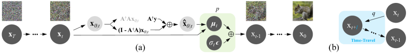
Figure 2: Illustration of (a) DDNM and (b) the time-travel trick.

3.2 Examples of Constructing $\mathbf{A}$ and $\mathbf{A}^{\dagger}$

Typical IR tasks usually have simple forms of $\mathbf{A}$ and $\mathbf{A}^{\dagger}$, some of which are easy to construct by hand without resorting to complex Fourier transform or SVD. Here we introduce three practical examples. Inpainting is the simplest case, where $\mathbf{A}$ is the mask operator. Due to the unique property that $\mathbf{A}\mathbf{A}\mathbf{A}\equiv\mathbf{A}$, we can use $\mathbf{A}$ itself as $\mathbf{A}^{\dagger}$. For colorization, $\mathbf{A}$ can be a pixel-wise operator $\begin{bmatrix}\frac{1}{3}&\frac{1}{3}&\frac{1}{3}\end{bmatrix}$ that converts each RGB channel pixel $\begin{bmatrix}r&g&b\end{bmatrix}^{\top}$ into a grayscale value $\begin{bmatrix}\frac{r}{3}+\frac{g}{3}+\frac{b}{3}\end{bmatrix}$. It is easy to construct a pseudo-inverse $\mathbf{A}^{\dagger}=\begin{bmatrix}1&1&1\end{bmatrix}^{\top}$ that satisfies $\mathbf{A}\mathbf{A}^{\dagger}\equiv\mathbf{I}$. The same idea can be used for SR with scale $n$, where we can set $\mathbf{A}\in\mathbb{R}^{1\times n^{2}}$ as the average-pooling operator $\begin{bmatrix}\frac{1}{n^{2}}&...&\frac{1}{n^{2}}\end{bmatrix}$ that averages each patch into a single value. Similarly, we can construct its pseudo-inverse as $\mathbf{A}^{\dagger}\in\mathbb{R}^{n^{2}\times 1}=\begin{bmatrix}1&...&1\end{bmatrix}^{\top}$. We provide pytorch-like codes in Appendix E.

Considering $\mathbf{A}$ as a compound operation that consists of many sub-operations, i.e., $\mathbf{A}=\mathbf{A}_{1}...\mathbf{A}_{n}$, we may still yield its pseudo-inverse $\mathbf{A}^{\dagger}=\mathbf{A}_{n}^{\dagger}...\mathbf{A}_{1}^{\dagger}$. This provides a flexible solution for solving complex IR tasks, such as old photo restoration. Specifically, we can decompose the degradation of old photos as three parts, i.e., $\mathbf{A}=\mathbf{A}_{1}\mathbf{A}_{2}\mathbf{A}_{3}$, where $\mathbf{A}_{3}$ is the grayscale operator, $\mathbf{A}_{2}$ is the average-pooling operator with scale 4, and $\mathbf{A}_{1}$ is the mask operator defined by the damaged areas on the photo. Hence the pseudo-inverse is $\mathbf{A}^{\dagger}=\mathbf{A}_{3}^{\dagger}\mathbf{A}_{2}^{\dagger}\mathbf{A}_{1}^{\dagger}$. Our experiments show that these hand-designed operators work very well (Fig. 1(a,b,d)).

3.3 Enhanced Version: DDNM⁺

DDNM can solve noise-free IR tasks well but fails to handle noisy IR tasks and yields poor Realness in the face of some particular forms of $\mathbf{A}^{\dagger}$. To overcome these two limits, as described by Algo. 2, we propose an enhanced version, dubbed DDNM⁺, by making the following two major extensions to DDNM to enable it to handle noisy situations and improve its restoration quality.

Scaling Range-Space Correction to Support Noisy Image Restoration

We consider noisy IR problems in the form of $\mathbf{y}$$=$$\mathbf{A}\mathbf{x}+{\color[rgb]{0,0,1}\mathbf{n}}$, where $\mathbf{n}$$\in$$\mathbb{R}^{d\times 1}$$\sim$$\mathcal{N}(\mathbf{0},\sigma_{\mathbf{y}}^{2}\mathbf{I})$ represents the additive Gaussian noise and $\mathbf{A}\mathbf{x}$ represents the clean measurement. Applying DDNM directly yields

$$\mathbf{\hat{x}}_{0|t}=\mathbf{A^{\dagger}}\mathbf{y}+(\mathbf{I}-\mathbf{A^{\dagger}}\mathbf{A})\mathbf{x}_{0|t}=\mathbf{x}_{0|t}-\mathbf{A}^{\dagger}(\mathbf{A}\mathbf{x}_{0|t}-\mathbf{A}\mathbf{x})+{\color[rgb]{0,0,1}\mathbf{A}^{\dagger}\mathbf{n}},$$ (16)

where ${\color[rgb]{0,0,1}\mathbf{A}^{\dagger}\mathbf{n}}\in\mathbb{R}^{D\times 1}$ is the extra noise introduced into $\mathbf{\hat{x}}_{0|t}$ and will be further introduced into $\mathbf{x}_{t-1}$. $\mathbf{A}^{\dagger}(\mathbf{A}\mathbf{x}_{0|t}-\mathbf{A}\mathbf{x})$ is the correction for the range-space contents, which is the key to Consistency. To solve noisy image restoration, we propose to modify DDNM (on Eq. 13 and Eq. 14) as:

$$\mathbf{\hat{x}}_{0|t}=\mathbf{x}_{0|t}-{\color[rgb]{0,0,1}\mathbf{\Sigma}_{t}}\mathbf{A}^{\dagger}(\mathbf{A}\mathbf{x}_{0|t}-\mathbf{y}),$$ (17)

$${\color[rgb]{0,0,1}\hat{p}}(\mathbf{x}_{t-1}|\mathbf{x}_{t},\mathbf{\hat{x}}_{0|t})=\mathcal{N}(\mathbf{x}_{t-1};\bm{\mu}_{t}(\mathbf{x}_{t},\mathbf{\hat{x}}_{0|t}),{\color[rgb]{0,0,1}\mathbf{\Phi}_{t}}\mathbf{I}).$$ (18)

${\color[rgb]{0,0,1}\mathbf{\Sigma}_{t}}\in\mathbb{R}^{D\times D}$ is utilized to scale the range-space correction $\mathbf{A}^{\dagger}(\mathbf{A}\mathbf{x}_{0|t}-\mathbf{y})$ and ${\color[rgb]{0,0,1}\mathbf{\Phi}_{t}}\in\mathbb{R}^{D\times D}$ is used to scale the added noise $\sigma_{t}\bm{\epsilon}$ in $p(\mathbf{x}_{t-1}|\mathbf{x}_{t},\mathbf{\hat{x}}_{0|t})$. The choice of ${\color[rgb]{0,0,1}\mathbf{\Sigma}_{t}}$ and ${\color[rgb]{0,0,1}\mathbf{\Phi}_{t}}$ follows two principles: (i) ${\color[rgb]{0,0,1}\mathbf{\Sigma}_{t}}$ and ${\color[rgb]{0,0,1}\mathbf{\Phi}_{t}}$ need to assure the total noise variance in $\mathbf{x}_{t-1}$ conforms to the definition in $q(\mathbf{x}_{t-1}|\mathbf{x}_{0})$ (Eq. 5) so the total noise can be predicted by $\mathcal{Z}_{\bm{\theta}}$ and gets removed; (ii) ${\color[rgb]{0,0,1}\mathbf{\Sigma}_{t}}$ should be as close as possible to $\mathbf{I}$ to maximize the preservation of the range-space correction $\mathbf{A}^{\dagger}(\mathbf{A}\mathbf{x}_{0|t}-\mathbf{y})$ so as to maximize the Consistency. For SR and colorization defined in Sec.3.2, $\mathbf{A}^{\dagger}$ is copy operation. Thus $\mathbf{A}^{\dagger}\mathbf{n}$ can be approximated as a Gaussian noise $\mathcal{N}(\mathbf{0},\sigma_{\mathbf{y}}^{2}\mathbf{I})$, then $\mathbf{\Sigma}_{t}$ and $\mathbf{\Phi}_{t}$ can be simplified as $\mathbf{\Sigma}_{t}={\color[rgb]{0,0,1}\lambda_{t}}\mathbf{I}$ and $\mathbf{\Phi}_{t}={\color[rgb]{0,0,1}\gamma_{t}}\mathbf{I}$. Since $\mathbf{x}_{t-1}=\frac{\sqrt{\bar{\alpha}_{t-1}}\beta_{t}}{1-\bar{\alpha}_{t}}\hat{\mathbf{x}}_{0|t}+\frac{\sqrt{\alpha_{t}}(1-\bar{\alpha}_{t-1})}{1-\bar{\alpha}_{t}}\mathbf{x}_{t}+\sigma_{t}\bm{\epsilon}$, principle (i) is equivalent to: $(a_{t}{\color[rgb]{0,0,1}\lambda_{t}}\sigma_{\mathbf{y}})^{2}+{\color[rgb]{0,0,1}\gamma_{t}}\equiv\sigma_{t}^{2}$ with $a_{t}$ denotes $\frac{\sqrt{\bar{\alpha}_{t-1}}\beta_{t}}{1-\bar{\alpha}_{t}}$. Considering principle (ii), we set:

$${\color[rgb]{0,0,1}\gamma_{t}}=\sigma_{t}^{2}-(a_{t}{\color[rgb]{0,0,1}\lambda_{t}}\sigma_{\mathbf{y}})^{2},\quad{\color[rgb]{0,0,1}\lambda_{t}}=\begin{cases}1,&\sigma_{t}\geq a_{t}\sigma_{\mathbf{y}}\\ \sigma_{t}/a_{t}\sigma_{\mathbf{y}},&\sigma_{t}<a_{t}\sigma_{\mathbf{y}}\end{cases}.$$ (19)

In addition to the simplified version above, we also provide a more accurate version for general forms of $\mathbf{A}^{\dagger}$, where we set ${\color[rgb]{0,0,1}\mathbf{\Sigma}_{t}}=\mathbf{V}diag\{\lambda_{t1},\dots,\lambda_{tD}\}\mathbf{V}^{\top}$, ${\color[rgb]{0,0,1}\mathbf{\Phi}_{t}}=\mathbf{V}diag\{\gamma_{t1},\dots,\gamma_{tD}\}\mathbf{V}^{\top}$. $\mathbf{V}$ is derived from the SVD of the operator $\mathbf{A}(=\mathbf{U}\mathbf{\Sigma}\mathbf{V}^{\top})$. The calculation of $\lambda_{ti}$ and $\gamma_{ti}$ are presented in Appendix  I. Note that the only hyperparameter that need manual setting is $\sigma_{\mathbf{y}}$.

We can also approximate non-Gaussian noise like Poisson, speckle, and real-world noise as Gaussian noise, thereby estimating a noise level $\sigma_{\mathbf{y}}$ and resorting to the same solution mentioned above.

Time-Travel For Better Restoration Quality

We find that DDNM yields inferior Realness when facing particular cases like SR with large-scale average-pooling downsampler, low sampling ratio compressed sensing(CS), and inpainting with a large mask. In these cases, the range-space contents $\mathbf{A}^{\dagger}\mathbf{y}$ is too local to guide the reverse diffusion process toward yielding a global harmony result.

Let us review Eq. 11. We can see that the mean value $\bm{\mu}_{t}(\mathbf{x}_{t},\mathbf{x}_{0})$ of the posterior distribution $p(\mathbf{x}_{t-1}|\mathbf{x}_{t},\mathbf{x}_{0})$ relies on accurate estimation of $\mathbf{x}_{0}$. DDNM uses $\hat{\mathbf{x}}_{0|t}$ as the estimation of $\mathbf{x}_{0}$ at time-step $t$, but if the range-space contents $\mathbf{A}^{\dagger}\mathbf{y}$ is too local or uneven, $\hat{\mathbf{x}}_{0|t}$ may have disharmonious null-space contents. How can we salvage the disharmony? Well, we can time travel back to change the past. Say we travel back to time-step $t+{\color[rgb]{0,0,1}l}$, we can yield the next state $\mathbf{x}_{t+{\color[rgb]{0,0,1}l}-1}$ using the “future” estimation $\hat{\mathbf{x}}_{0|t}$, which should be more accurate than $\hat{\mathbf{x}}_{0|t+{\color[rgb]{0,0,1}l}}$. By reparameterization, this operation is equivalent to sampling $\mathbf{x}_{t+{\color[rgb]{0,0,1}l}-1}$ from $q(\mathbf{x}_{t+{\color[rgb]{0,0,1}l}-1}|\mathbf{x}_{t-1})$. Similar to Lugmayr et al. (2022) that use a “back and forward” strategy for inpainting tasks, we propose a time-travel trick to improve global harmony for general IR tasks: For a chosen time-step $t$, we sample $\mathbf{x}_{t+{\color[rgb]{0,0,1}l}}$ from $q(\mathbf{x}_{t+{\color[rgb]{0,0,1}l}}|\mathbf{x}_{t})$. Then we travel back to time-step $t+{\color[rgb]{0,0,1}l}$ and repeat normal DDNM sampling (Eq. 12, Eq. 13, and Eq. 14) until yielding $\mathbf{x}_{t-1}$. ${\color[rgb]{0,0,1}l}$ is actually the travel length. Fig. 2(b) illustrates the basic time-travel trick.

Intuitively, the time-travel trick produces a better “past”, which in turn produces a better “future”. For ease of use, we assign two extra hyperparameters: $s$ controls the interval of using the time-travel trick; $r$ determines the repeat times. The time-travel trick in Algo. 2 is with $s=1$, $r=1$. Fig. 4(b) and the right part in Tab. 4 demonstrate the improvements that the time-travel trick brings.

It is worth emphasizing that although Algo. 1 and Algo. 2 are derived based on DDPM, they can also be easily extended to other diffusion frameworks, such as DDIM (Song et al., 2021a). Obviously, DDNM⁺ becomes exactly DDNM when setting $\mathbf{\Sigma}_{t}=\mathbf{I}$, $\mathbf{\Phi}_{t}=\sigma_{t}^{2}\mathbf{I}$, and $l=0$.

ImageNet	4$\times$ SR	Deblurring	Colorization	CS 25%	Inpainting
Method	PSNR↑/SSIM↑/FID↓	PSNR↑/SSIM↑/FID↓	Cons↓/FID↓	PSNR↑/SSIM↑/FID↓	PSNR↑/SSIM↑/FID↓
$\mathbf{A}^{\dagger}\mathbf{y}$	24.26 / 0.684 / 134.4	18.56 / 0.6616 / 55.42	0.0 / 43.37	15.65 / 0.510 / 277.4	14.52 / 0.799 / 72.71
DGP	23.18 / 0.798 / 64.34	N/A	- / 69.54	N/A	N/A
ILVR	27.40 / 0.870 / 43.66	N/A	N/A	N/A	N/A
RePaint	N/A	N/A	N/A	N/A	31.87 / 0.968 / 12.31
DDRM	27.38 / 0.869 / 43.15	43.01 / 0.992 / 1.48	260.4 / 36.56	19.95 / 0.704 / 97.99	31.73 / 0.966 / 4.82
DDNM(ours)	27.46 / 0.870/ 39.26	44.93 / 0.994 / 1.15	42.32 / 36.32	21.66 / 0.749 / 64.68	32.06 / 0.968 / 3.89

CelebA	4$\times$ SR	Deblurring	Colorization	CS 25%	Inpainting
Method	PSNR↑/SSIM↑/FID↓	PSNR↑/SSIM↑/FID↓	Cons↓/FID↓	PSNR↑/SSIM↑/FID↓	PSNR↑/SSIM↑/FID↓
$\mathbf{A}^{\dagger}\mathbf{y}$	27.27 / 0.782 / 103.3	18.85 / 0.741 / 54.31	0.0 / 68.81	15.09 / 0.583 / 377.7	15.57 / 0.809 / 181.56
PULSE	22.74 / 0.623 / 40.33	N/A	N/A	N/A	N/A
ILVR	31.59 / 0.945 / 29.82	N/A	N/A	N/A	N/A
RePaint	N/A	N/A	N/A	N/A	35.20 / 0.981 /14.19
DDRM	31.63 / 0.945 / 31.04	43.07 / 0.993 / 6.24	455.9 / 31.26	24.86 / 0.876 / 46.77	34.79 / 0.978 /12.53
DDNM(ours)	31.63 / 0.945 / 22.27	46.72 / 0.996 / 1.41	26.25 / 26.44	27.56 / 0.909 / 28.80	35.64 / 0.982 /4.54

Table 1: Quantitative results of zero-shot IR methods on ImageNet(top) and CelebA(bottom), including five typical IR tasks. We mark N/A for those not applicable and bold the best scores.

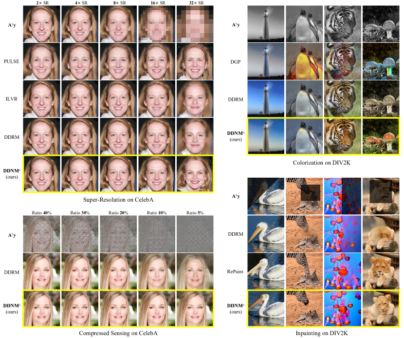
Figure 3: Qualitative results of zero-shot IR methods.

4 Experiments

Our experiments consist of three parts. Firstly, we evaluate the performance of DDNM on five typical IR tasks and compare it with state-of-the-art zero-shot IR methods. Secondly, we experiment DDNM⁺ on three typical IR tasks to verify its improvements against DDNM. Thirdly, we show that DDNM and DDNM⁺ perform well on challenging real-world applications.

4.1 Evaluation on DDNM

To evaluate the performance of DDNM, we compare DDNM with recent state-of-the-art zero-shot IR methods: DGP(Chen & Davies, 2020), Pulse(Menon et al., 2020), ILVR(Choi et al., 2021), RePaint(Lugmayr et al., 2022) and DDRM(Kawar et al., 2022). We experiment on five typical noise-free IR tasks, including 4$\times$ SR with bicubic downsampler, deblurring with Gaussian blur kernel, colorization with average grayscale operator, compressed sensing (CS) using Walsh-Hadamard sampling matrix with a 0.25 compression ratio, and inpainting with text masks. For each task, we use the same degradation operator for all methods. We choose ImageNet 1K and CelebA 1K datasets with image size 256$\times$256 for validation. For ImageNet 1K, we use the 256$\times$256 denoising network as $\mathcal{Z}_{\bm{\theta}}$, which is pretrained on ImageNet by Dhariwal & Nichol (2021). For CelebA 1K, we use the 256$\times$256 denoising network pretrained on CelebA by Lugmayr et al. (2022). For fair comparisons, we use the same pretrained denoising networks for ILVR, RePaint, DDRM, and DDNM. We use DDIM as the base sampling strategy with $\eta=0.85$, 100 steps, without classifier guidance, for all diffusion-based methods. We choose PSNR, SSIM, and FID (Heusel et al., 2017) as the main metrics. Since PSNR and SSIM can not reflect the colorization performance, we use FID and the Consistency metric (calculated by $||\mathbf{A}\mathbf{x}_{0}-\mathbf{y}||_{1}$ and denoted as Cons) for colorization.

Tab. 1 shows the quantitative results. For those tasks that are not supported, we mark them as “NA”. We can see that DDNM far exceeds previous GAN prior based zero-shot IR methods (DGP, PULSE). Though with the same pretrained denoising models and sampling steps, DDNM achieves significantly better performance in both Consistency and Realness than ILVR, RePaint, and DDRM. Appendix  J shows more quantitative comparisons and qualitative results.

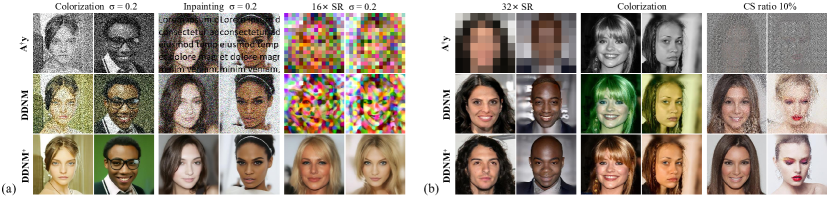
Figure 4: DDNM⁺ improves (a) denoising performance and (b) restoration quality.

CelebA	16$\times$ SR $\sigma$=0.2	C $\sigma$=0.2	CS ratio=25% $\sigma$=0.2	32$\times$ SR	C	CS ratio=10%
Method	PSNR↑/SSIM↑/FID↓	FID↓	PSNR↑/SSIM↑/FID↓	PSNR↑/SSIM↑/FID↓	FID↓	PSNR↑/SSIM↑/FID↓
DDNM	13.10 / 0.2387 / 281.45	216.74	17.89 / 0.4531 / 82.81	17.55 / 0.437 / 39.37	22.79	15.74/ 0.275 / 110.7
DDNM+	19.44 / 0.712 / 58.31	46.11	25.02 / 0.868 / 51.35	18.44 / 0.501 / 37.50	18.23	26.33 / 0.741 / 47.93

Table 2: Ablation study on denoising improvements (left) and the time-travel trick (right). C represents the colorization task. $\sigma$ denotes the noise variance on $\mathbf{y}$.

4.2 Evaluation on DDNM⁺

We evaluate the performance of DDNM⁺ from two aspects: the denoising performance and the robustness in restoration quality.

Denoising Performance. We experiment DDNM⁺ on three noisy IR tasks with $l=0$, i.e., we disable the time-travel trick to only evaluate the denoising performance. Fig. 4(a) and the left part in Tab. 2 show the denoising improvements of DDNM⁺ against DDNM. We can see that DDNM fully inherits the noise contained in $\mathbf{y}$, while DDNM⁺ decently removes the noise.

Robustness in Restoration Quality. We experiment DDNM⁺ on three tasks that DDNM may yield inferior results, they are 32$\times$ SR, colorization, and compressed sensing (CS) using orthogonalized sampling matrix with a 10% compression ratio. For fair comparison, we set $T=250$, $l=s=20$, $r=3$ for DDNM⁺ while set $T=1000$ for DDNM so that the total sampling steps and computational consumptions are roughly equal. Fig. 4(b) and the right part in Tab. 2 show the improvements of the time-travel trick. We can see that the time-travel trick significantly improves the overall performance, especially the Realness (measured by FID).

To the best of our knowledge, DDNM⁺ is the first IR method that can robustly handle arbitrary scales of linear IR tasks. As is shown in Fig. 3, We compare DDNM⁺ ($l=s=10$, $r=5$) with state-of-the-art zero-shot IR methods on diverse IR tasks. We also crop images from DIV2K dataset (Agustsson & Timofte, 2017) as the testset. The results show that DDNM⁺ owns excellent robustness in dealing with diverse IR tasks, which is remarkable considering DDNM⁺ as a zero-shot method. More experiments of DDNM/DDNM⁺ can be found in Appendix A and B.

4.3 Real-World Applications

Theoretically, we can use DDNM⁺ to solve real-world IR task as long as we can construct an approximate linear degradation $\mathbf{A}$ and its pseudo-inverse $\mathbf{A}^{\dagger}$. Here we demonstrate two typical real-world applications using DDNM⁺ with $l=s=20$, $r=3$: (1) Real-World Noise. We experiment DDNM⁺ on real-world colorization with $\mathbf{A}$ and $\mathbf{A}^{\dagger}$ defined in Sec. 3.2. We set $\sigma_{\mathbf{y}}$ by observing the noise level of $\mathbf{y}$. The results are shown in Fig. 7, Fig. 8, and Fig. 1(c). (2) Old Photo Restoration. For old photos, we construct $\mathbf{A}$ and $\mathbf{A}^{\dagger}$ as described in Sec  3.2, where we manually draw a mask for damaged areas on the photo. The results are shown in Fig. 1(d), and Fig. 16.

5 Related Work

5.1 Diffusion Models for Image Restoration

Recent methods using diffusion models to solve image restoration can be roughly divided into two categories: supervised methods and zero-shot methods.

Supervised Methods. SR3 (Saharia et al., 2021) trains a conditional diffusion model for image super-resolution with synthetic image pairs as the training data. This pattern is further promoted to other IR tasks (Saharia et al., 2022). To solve image deblurring, Whang et al. (2022) uses a deterministic predictor to estimate the initial result and trains a diffusion model to predict the residual. However, these methods all need task-specific training and can not generalize to different degradation operators or different IR tasks.

Zero-Shot Methods. Song & Ermon (2019) first propose a zero-shot image inpainting solution by guiding the reverse diffusion process with the unmasked region. They further propose using gradient guidance to solve general inverse problems in a zero-shot fashion and apply this idea to medical imaging problems (Song et al., 2020; 2021b). ILVR (Choi et al., 2021) applies low-frequency guidance from a reference image to achieve reference-based image generation tasks. RePaint (Lugmayr et al., 2022) solves the inpainting problem by guiding the diffusion process with the unmasked region. DDRM (Kawar et al., 2022) uses SVD to decompose the degradation operators. However, SVD encounters a computational bottleneck when dealing with high-dimensional matrices. Actually, the core guidance function in ILVR (Choi et al., 2021), RePaint (Lugmayr et al., 2022) and DDRM (Kawar et al., 2022) can be seen as special cases of the range-null space decomposition used in DDNM, detailed analysis is in Appendix  H.

5.2 Range-Null Space Decomposition in Image Inverse Problems

Schwab et al. (2019) first proposes using a DNN to learn the missing null-space contents in image inverse problems and provide detailed theory analysis. Chen & Davies (2020) proposes learning the range and null space respectively. Bahat & Michaeli (2020) achieves editable super-resolution via exploring the null-space contents. Wang et al. (2022a) apply range-null space decomposition to existing GAN prior based SR methods to improve their performance and convergence speed.

6 Conclusion & Discussion

This paper presents a unified framework for solving linear IR tasks in a zero-shot manner. We believe that our work demonstrates a promising new path for solving general IR tasks, which may also be instructive for general inverse problems. Theoretically, our framework can be easily extended to solve inverse problems of diverse data types, e.g., video, audio, and point cloud, as long as one can collect enough data to train a corresponding diffusion model. More discussion is in Appendix C.

Figure 5: 4$\times$SR using Mask-Shift trick, DDNM. Input size: 64$\times$256; output size: 256$\times$1024.

7 Mask-Shift Trick

In this section, we propose a Mask-Shift trick that enables DDNM to solve IR tasks with arbitrary desired output sizes, e.g., 4K images.

Diffusion models usually have a strict constraint on output image size. Assume the default DDNM yields results of size 256$\times$256. We have a low-resolution image $\mathbf{y}$ with size 64$\times$256 and want to SR it into size 256$\times$1024. The simplest way is to divide $\mathbf{y}$ into 4 images with resolution 64$\times$64, then use DDNM to yield 4 SR results and concatenate them as the final result. However, this will bring significant block artifacts between each division.

Here we propose a simple but effective trick to perfectly solve this problem. Let’s take the above example. First, we divide $\mathbf{y}$ into 8 parts [$\mathbf{y}^{(0)},...,\mathbf{y}^{(7)}$], each part is a 64$\times$32 image. In the first turn, we take [$\mathbf{y}^{(0)}$,$\mathbf{y}^{(1)}$] as the input and use DDNM to get the SR result $\mathbf{x}$, we further divide it as [$\mathbf{x}^{(0)}$,$\mathbf{x}^{(1)}$]. Next, we need to run 6 turns of DDNM. For the $i$th turn, we use [$\mathbf{y}^{(i)}$,$\mathbf{y}^{(i+1)}$] as the input and divide the intermediate result $\hat{\mathbf{x}}_{0|t}$ as [$\hat{\mathbf{x}}_{0|t}^{(left)},\hat{\mathbf{x}}_{0|t}^{(right)}$] and replace its left by

$$\hat{\mathbf{x}}_{0|t}=[\mathbf{x}^{(i)},\hat{\mathbf{x}}_{0|t}^{(right)}],$$ (20)

The final result is $\mathbf{x}_{0}=$[$\mathbf{x}^{(0)}$, …, $\mathbf{x}^{(7)}$], as shown in Fig. 5. This method assures the reconstruction is always coherent between shifts. We call it the Mask-Shift trick. For input image $\mathbf{y}$ with an arbitrary size, we can first zero-pad it into regular size, then divide it vertically and horizontally. Then use a similar Mask-Shift trick to ensure the vertical and horizontal coherence of the final output result.

Appendix A Time & Memory Consumption

Our method has obvious advantages in time & memory consumption among recent zero-shot diffusion-based restoration methods (Kawar et al., 2022; Ho et al., 2022; Chung et al., 2022b; a). These methods are all based on basic diffusion models, the differences are how to bring the constraint $\mathbf{y}=\mathbf{Ax}+\mathbf{n}$ into the reverse diffusion process. We conclude our advantages as below:

• DDNM yields almost the same consumption as the original diffusion models.

• DDNM does not need any optimization toward minimizing $||\mathbf{y}-\mathbf{A}\mathbf{x}_{0|t}||$ since we directly yield the optimal solution by range-null space decomposition (Section 3.1) and precise range-space denoising (Section 3.3). We notice some recent works (Ho et al., 2022; Chung et al., 2022b; a) resort to such optimization, e.g., DPS (Chung et al., 2022a) uses $\mathbf{x}_{t-1}=\mathbf{x}_{t-1}-\zeta_{t}\nabla_{\mathbf{x}_{t}}||\mathbf{y}-\mathbf{A}\mathbf{x}_{0|t}||^{2}_{2}$ to update $\mathbf{x}_{t-1}$; however, this involves costly gradient computation.

• Unlike DDRM (Kawar et al., 2022), our DDNM does not necessarily need SVD. As is presented in Section 3.2, we construct $\mathbf{A}$ and $\mathbf{A}^{\dagger}$ for colorization, inpainting, and super-resolution problems by hand, which bring negligible computation and memory consumption. In contrast, SVD-based methods suffer heavy cost on memory and computation if $\mathbf{A}$ has a high dimension (e.g., 128xSR, as shown below).

Experiments in Tab. 3 well support these claims.

ImageNet	4$\times$ SR				64$\times$ SR		128$\times$ SR
Method	PSNR↑	FID↓	Time(s/image)	Memory(MB)	Time	Memory	Time	Memory
DDPM*	N/A	N/A	11.9	5758	11.9	5758	11.9	5758
DPS	25.51	55.92	36.5	8112	-	-	-	-
DDRM	27.05	38.05	12.4	5788	36.4	5788	83.3	6792
DDNM	27.04	33.81	11.9	5728	11.9	5728	11.9	5728

Table 3: Comparisons on Time & Memory Consumption. We use the average-pooling downsampler, 4$\times$ SR, 100 DDIM steps with $\eta$=0.85 and without classifier guidance, on a single 2080Ti GPU with batch size 1. For DPS, we set $\zeta_{t}$=100$\sqrt{\bar{\alpha}_{t-1}}$. *The DDPM here is tested on unconditional generation.

Appendix B Comparing DDNM with Supervised Methods

Our method is superior to existing supervised IR methods (Zhang et al., 2021; Liang et al., 2021) in these ways:

• DDNM is zero-shot for diverse tasks, but supervised methods need to train separate models for each task.

• DDNM is robust to degradation modes, but supervised methods own poor generalized performance.

• DDNM yields significantly better performance on certain datasets and resolutions (e.g., ImageNet at 256x256).

These claims are well supported by experiments in Tab. 4.

ImageNet	Bicubic, $\sigma_{\mathbf{y}}$=0			Average-pooling, $\sigma_{\mathbf{y}}$=0			Average-pooling, $\sigma_{\mathbf{y}}$=0.2			Inference time
Method	PSNR↑	SSIM↑	FID↓	PSNR↑	SSIM↑	FID↓	PSNR↑	SSIM↑	FID↓	s/image
SwinIR-L	21.21	0.7410	56.77	23.88	0.8010	54.93	18.39	0.5387	134.18	6.1
BSRGAN	21.46	0.7384	68.15	24.14	0.7948	67.70	14.06	0.3663	195.41	0.036
DDNM	27.46	0.8707	39.26	27.04	0.8651	33.81	22.67	0.7400	80.69	11.9

Table 4: Comparisons between DDNM and supervised SR methods. DDNM uses 100 DDIM steps with $\eta$=0.85 and without classifier guidance. We use the official SwinIR-L (Liang et al., 2021) and BSRGAN (Zhang et al., 2021) pretrained for SR tasks.

Appendix C Limitations

There remain many limitations that deserve further study.

• Though DDNM brings negligible extra cost on computations, it is still limited by the slow inference speed of existing diffusion models.

• DDNM needs explicit forms of the degradation operator, which may be challenging to acquire for some tasks. Approximations may work well, but not optimal.

• In theory, DDNM only supports linear operators. Though nonlinear operators may also have “pseudo-inverse”, they may not conform to the distributive property, e.g., $\sin(a+b)\neq\sin(a)+\sin(b)$, so they may not have linearly separable null-space and range-space.

• DDNM inherits the randomness of diffusion models. This property benefits diversity but may yield undesirable results sometimes.

• The restoration capabilities of DDNM are limited by the performance of the pretrained denoiser, which is related to the network capacity and the training dataset. For example, existing diffusion models do not outperform StyleGANs (Karras et al., 2019; 2020; 2021) in synthesizing FFHQ/AFHQ images at 1024$\times$1024 resolution.

Appendix D Solving Real-World Degradation Using DDNM⁺

DDNM+ can well handle real-world degradation, where the degradation operator A is unknown and non-linear and even contains non-Gaussian noise. We follow these observations:

• In theory, DDNM⁺ is designed to solve IR tasks of diverse noise levels. As is shown in Fig. 6, DDNM⁺ can well handle 4$\times$ SR even with a strong noise $\sigma_{\mathbf{y}}$=0.9.

• For real-world degraded images, the non-linear artifacts can generally be divided into global (e.g., the real-world noise in Fig. 1(c)) and local (e.g., the scratches in Fig. 1(d)).

• For global non-linear artifacts, we can set a proper $\mathbf{\sigma_{\mathbf{y}}}$ to cover them. As is shown in Fig. 7, the input images $\mathbf{y}$ suffer JPEG-like unknown artifacts, but DDNM⁺ can still remove them decently by setting a proper $\mathbf{\sigma_{\mathbf{y}}}$.

• For local non-linear artifacts, we can directly draw a mask to cover them. Hence all we need is to construct $\mathbf{A}=\mathbf{A}_{color}\mathbf{A}_{mask}$ and set a proper $\sigma_{\mathbf{y}}$. We have proved $\mathbf{A}_{color}$ and $\mathbf{A}_{mask}$ and their pseudo-inverse can be easily constructed by hand. (maybe a $\mathbf{A}_{SR}$ is needed for resize when $\mathbf{y}$ is too blur)

Figure 6: DDNM⁺ can well handle 4$\times$ SR even with a strong noise $\sigma_{\mathbf{y}}$=0.9.

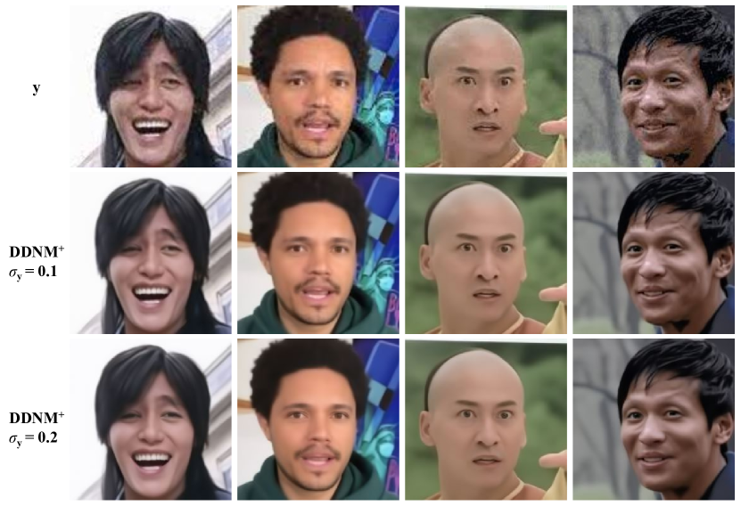
Figure 7: Solving JPEG-like artifacts using DDNM⁺. Here we set $\mathbf{A}=\mathbf{I}$ to exert a pure denoising. $\mathbf{y}$ denotes the input degraded image. When we set $\mathbf{\sigma_{\mathbf{y}}}=0.1$, the artifacts are decently removed. When we set $\mathbf{\sigma_{\mathbf{y}}}=0.2$, the results become smoother but yield relatively poor identity consistency.

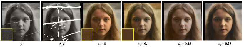
Figure 8: Old photo restoration. Zoom in for the best view. By setting $\mathbf{\sigma_{\mathbf{y}}}=0.1$, the noise is removed, and the identity is well preserved. When we set higher $\mathbf{\sigma_{\mathbf{y}}}=0.25$, the results becomes much smoother but yield relatively poor identity consistency.

In Fig. 8 we demonstrate an example. The input image $\mathbf{y}$ is a black-and-white photo with unknown noise and scratches. We first manually draw a mask $\mathbf{A_{mask}}$ to cover these scratches. Then we use a grayscale operator $\mathbf{A_{color}}$ to convert the image into grayscale. Definition of $\mathbf{A_{mask}}$ and $\mathbf{A_{color}}$ and their pseudo-inverse can be find in Sec. 3.2. Then we take $\mathbf{A}=\mathbf{A_{color}}\mathbf{A_{mask}}$ and $\mathbf{A}^{\dagger}=\mathbf{A_{mask}}^{\dagger}\mathbf{A_{color}}^{\dagger}$ for DDNM⁺, and set a proper $\mathbf{\sigma_{\mathbf{y}}}$. From the results in Fig. 8, we can see that when setting $\mathbf{\sigma_{\mathbf{y}}}=0$, the noise is fully inherited by the results. By setting $\mathbf{\sigma_{\mathbf{y}}}=0.1$, the noise is removed, and the identity is well preserved. When we set higher $\mathbf{\sigma_{\mathbf{y}}}=0.25$, the results becomes much smoother but yield relatively poor identity consistency.

The choice of $\mathbf{\sigma_{\mathbf{y}}}$ is critical to achieve the best balance between realness and consistency. But for now we can only rely on manual estimates.

Appendix E PyTorch-Like Code Implementation

Here we provide a basic PyTorch-Like implementation of DDNM⁺. Readers can quickly implement a basic DDNM⁺ on their own projects by referencing Algo. 2 and Sec. 3.3 and the code below.

⬇

1

def color2gray(x):

3 coef=1/3

x = x[:,0,:,:] * coef + x[:,1,:,:]*coef + x[:,2,:,:]*coef

5 return x.repeat(1,3,1,1)

7def gray2color(x):

x = x[:,0,:,:]

9 coef=1/3

base = coef**2 + coef**2 + coef**2

11 return th.stack((x*coef/base, x*coef/base, x*coef/base), 1)

13def PatchUpsample(x, scale):

n, c, h, w = x.shape

15 x = torch.zeros(n,c,h,scale,w,scale) + x.view(n,c,h,1,w,1)

return x.view(n,c,scale*h,scale*w)

17

# Implementation of A and its pseudo-inverse Ap

19

if IR_mode==”colorization”:

21 A = color2gray

Ap = gray2color

23

elif IR_mode==”inpainting”:

25 A = lambda z: z*mask

Ap = A

27

elif IR_mode==”super resolution”:

29 A = torch.nn.AdaptiveAvgPool2d((256//scale,256//scale))

Ap = lambda z: PatchUpsample(z, scale)

31

elif IR_mode==”old photo restoration”:

33 A1 = lambda z: z*mask

A1p = A1

35

A2 = color2gray

37 A2p = gray2color

39 A3 = torch.nn.AdaptiveAvgPool2d((256//scale,256//scale))

A3p = lambda z: PatchUpsample(z, scale)

41

A = lambda z: A3(A2(A1(z)))

43 Ap = lambda z: A1p(A2p(A3p(z)))

45

# Core Implementation of DDNM+, simplified denoising solution

47# For more accurate denoising, please refer to Appendix I and the full source code.

49def ddnmp_core(x0t, y, sigma_y, sigma_t, a_t):

51 #Eq 19

if sigma_t >= a_t*sigma_y:

53 lambda_t = 1

gamma_t = sigma_t**2 - (a_t*lambda_t*sigma_y)**2

55 else:

lambda_t = sigma_t/(a_t*sigma_y)

57 gamma_t = 0

59 #Eq 17

x0t= x0t + lambda_t*Ap(y - A(x0t))

61

return x0t, gamma_t

Appendix F Details of The Degradation Operators

Super Resolution (SR).

For SR experiments in Tab. 1, we use the bicubic downsampler as the degradation operator to ensure fair comparisons. For other cases in this paper, we use the average-pooling downsampler as the degradation operator, which is easy to get the pseudo-inverse as described in Sec. 3.2. Fig. 9(a) and Fig. 9(b) show examples of the bicubic operation and the average-pooling operation.

Inpainting.

We use text masks, random pixel-wise masks, and hand-drawn masks for inpainting experiments. Fig.9(d) demonstrates examples of different masks.

Deblurring.

For deblurring experiments, We use three typical kernels to implement blurring operations, including Gaussian blur kernel, uniform blur kernel, and anisotropic blur kernel. For Gaussian blur, the kernel size is 5 and kernel width is 10; For uniform blur kernel, the kernel size is 9; For anisotropic blur kernel, the kernel size is 9 and the kernel widths of each axis are 20 and 1. Fig.9(c) demonstrates the effect of these kernels.

Compressed Sensing (CS).

For CS experiments, we choose two types of sampling matrices: one is based on the Walsh-Hadamard transformation, and the other is an orthogonalized random matrix applied to the original image block-wisely. For the Walsh-Hadamard sampling matrix, we choose 50% and 25% as the sampling ratio. For the orthogonalized sampling matrix, we choose ratios from 40% to 5%. Fig.9(e) and (f) demonstrate the effects of the Walsh-Hadamard sampling matrix and orthogonalized sampling matrix with different CS ratios.

Colorization.

For colorization, we choose the degradation matrix $\mathbf{A}=\begin{bmatrix}\frac{1}{3}&\frac{1}{3}&\frac{1}{3}\end{bmatrix}$ for each pixel as we described in Sec. 3.2. Fig.9(g) demonstrates the example of colorization degradation.

Solve the Pseudo-Inverse Using SVD

Considering we have a linear operator $\mathbf{A}$, we need to compute its pseudo-inverse $\mathbf{A}^{\dagger}$ to implement the algorithm of the proposed DDNM. For some simple degradation like inpainting, colorization, and SR based on average pooling, the pseudo-inverse $\mathbf{A}^{\dagger}$ can be constructed manually, which has been discussed in Sec. 3.2. For general cases, we can use the singular value decomposition (SVD) of $\mathbf{A}(=\mathbf{U}\mathbf{\Sigma}\mathbf{V}^{\top})$ to compute the pseudo-inverse $\mathbf{A}^{\dagger}(=\mathbf{V}\mathbf{\Sigma}^{\dagger}\mathbf{U}^{\top})$ where $\mathbf{\Sigma}$ and $\mathbf{\Sigma}^{\dagger}$ have the following relationship:

$$\mathbf{\Sigma}=diag\{s_{1},s_{2},\cdots\} ,\mathbf{\Sigma}^{\dagger}=diag\{d_{1},d_{2},\cdots\},$$ (21)

$$d_{i}= \begin{cases}\frac{1}{s_{i}}&s_{i}\neq 0\\ 0&s_{i}=0\end{cases},$$ (22)

where $s_{i}$ means the $i$-th singular value of $\mathbf{A}$ and $d_{i}$ means the $i$-th diagonal element of $\mathbf{\Sigma}^{\dagger}$.

Appendix G Visualization of The Intermediate Results

In Fig. 10, we visualize the intermediate results of DDNM on 4$\times$ SR, 16$\times$ SR, and deblurring. Specifically, we show the noisy result $\mathbf{x}_{t}$, the clean estimation $\mathbf{x}_{0|t}$, and the rectified clean estimation $\hat{\mathbf{x}}_{0|t}$. The total diffusion step is 1000. From Fig. 10(a), we can see that due to the fixed range-space contents $\mathbf{A}^{\dagger}\mathbf{y}$, $\hat{\mathbf{x}}_{0|t}$ already owns meaningful contents in early stages while $\mathbf{x}_{t}$ and $\mathbf{x}_{0|t}$ contains limited information. But when $t=0$, we can observe that $\mathbf{x}_{0|0}$ contains much more details than $\mathbf{A}^{\dagger}\mathbf{y}$. These details are precisely the null-space contents. We may notice a potential speed-up trick here. For example, we can replace $\mathbf{x}_{0|t=100}$ with $\mathbf{A}^{\dagger}\mathbf{y}$ and start DDNM directly from $t=100$, which yields a 10 times faster sampling. We leave it to future work. From Fig. 10(b), we can see that the reverse diffusion process gradually restores images from low-frequency contours to high-frequency details.

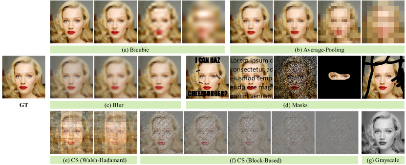
Figure 9: Visualization of different degradation operators. (a) Bicubic downsampler. The scale factors from left to right are $\times$4, $\times$8, $\times$16, $\times$32; (b) Average-pooling downsampler. The scale factors from left to right are $\times$4, $\times$8, $\times$16, $\times$32; (c) Blur operators. The type of kernels from left to right are Gaussian, uniform, and anisotropic; (d) Masks; (e) Walsh-Hadamard sampling matrix. The sampling ratios from left to right are 0.5 and 0.25; (f) Block-based sampling matrix. The sampling ratios from left to right are 0.4, 0.3, 0.2, 0.1, 0.05; (g) Grayscale operator.

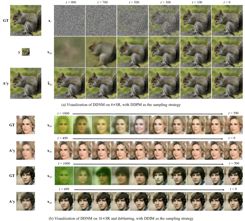
Figure 10: Visualization of the intermediate results in DDNM. Zoom-in for the best view.

Appendix H Comparing DDNM With Recent Diffusion-Based IR methods

Here we provide detailed comparison between DDNM and recent diffusion-based IR methods, including RePaint (Lugmayr et al., 2022), ILVR (Choi et al., 2021), DDRM (Kawar et al., 2022), SR3 (Saharia et al., 2021) and SDE (Song et al., 2020). For easier comparison, we rewrite their algorithms based on DDPM (Ho et al., 2020) and follow the characters used in DDNM. Algo. 3, Algo. 4 show the reverse diffusion process of DDPM and DDNM. We mark in blue those that are most distinct from DDNM. All the IR problems discussed here can be formulated as

$$\mathbf{y}=\mathbf{A}\mathbf{x}+\mathbf{n},$$ (23)

where $\mathbf{y}$, $\mathbf{A}$, $\mathbf{x}$, $\mathbf{n}$ represents the degraded image, the degradation operator, the original image, and the additive noise, respectively.

H.1 RePaint and ILVR.

RePaint (Lugmayr et al., 2022) solves noise-free image inpainting problems, where $\mathbf{n}=0$ and $\mathbf{A}$ represents the mask operation. RePaint first create a noised version of the masked image $\mathbf{y}$

$$\mathbf{y}_{t-1}=\mathbf{A}(\sqrt{\bar{\alpha}_{t-1}}\mathbf{y}+\sqrt{1-\bar{\alpha}_{t-1}}\bm{\epsilon}),\quad\bm{\epsilon}\sim\mathcal{N}(0,\mathbf{I}).$$ (24)

Then uses $\mathbf{y}_{t-1}$ to fill in the unmasked regions in $\mathbf{x}_{t-1}$:

$$\mathbf{x}_{t-1}=\mathbf{y}_{t-1}+(\mathbf{I}-\mathbf{A})\mathbf{x}_{t-1},$$ (25)

Besides, RePaint applies an “back and forward” strategy to refine the results. Algo. 5 shows the algorithm of RePaint.

ILVR (Choi et al., 2021) focuses on reference-based image generation tasks, where $\mathbf{n}=0$ and $\mathbf{A}$ represents a low-pass filter defined by $\mathbf{A}=\mathbf{A}_{1}\mathbf{A}_{2}$ ($\mathbf{A}_{1}$ is a bicubic upsampler and $\mathbf{A}_{2}$ is a bicubic downsampler). ILVR creates a noised version of the reference image $\mathbf{x}$ and uses the low-pass filter $\mathbf{A}$ to extract its low-frequency contents:

$$\mathbf{y}_{t-1}=\mathbf{A}(\sqrt{\bar{\alpha}_{t-1}}\mathbf{x}+\sqrt{1-\bar{\alpha}_{t-1}}\bm{\epsilon}),\quad\bm{\epsilon}\sim\mathcal{N}(0,\mathbf{I}).$$ (26)

Then combines the high-frequency part of $\mathbf{x}_{t-1}$ with the low-frequency contents in $\mathbf{y}_{t-1}$:

$$\mathbf{x}_{t-1}=\mathbf{y}_{t-1}+(\mathbf{I}-\mathbf{A})\mathbf{x}_{t-1},$$ (27)

Algo. 6 shows the algorithm of ILVR.

Essentially, RePaint and ILVR share the same formulations, with different definitions of the degradation operator $\mathbf{A}$. DDNM differs from RePaint and ILVR mainly in two parts:

(i) Operating on Different Domains. RePaint and ILVR all operate on the noisy $\mathbf{x}_{t}$ domain of diffusion models, which is inaccurate in range-space preservation during the reverse diffusion process. Instead, we directly operate on the noise-free $\mathbf{x}_{0|t}$ domain, which does not need extra process on $\mathbf{y}$ and is strictly derived from the theory and owns strict data consistency.

(ii) As Special Cases. Aside from the difference in operation domain, Eq. 25 of RePaint is essentially a special case of the range-null space decomposition. Considering $\mathbf{A}$ as a mask operator, it satisfies $\mathbf{A}\mathbf{A}\mathbf{A}=\mathbf{A}$, so we can use $\mathbf{A}$ itself as the pseudo-inverse $\mathbf{A}^{\dagger}$. Hence the range-null space decomposition becomes $\hat{\mathbf{x}}=\mathbf{A^{\dagger}}\mathbf{y}+(\mathbf{I}-\mathbf{A^{\dagger}}\mathbf{A})\bar{\mathbf{x}}=\mathbf{A}\mathbf{y}+(\mathbf{I}-\mathbf{A}\mathbf{A})\bar{\mathbf{x}}=\mathbf{y}+(\mathbf{I}-\mathbf{A})\bar{\mathbf{x}}$, which is exactly the same as Eq. 25. Similarly, Eq. 27 of ILVR can be seen as a special case of range-null space decomposition, which uses $\mathbf{I}$ as the approximation of $\mathbf{A}^{\dagger}$. Note that the final result $\mathbf{x}_{0}$ of RePaint satisfies Consistency, i.e., $\mathbf{A}\mathbf{x}_{0}\equiv\mathbf{y}$, while ILVR does not because the pseudo-inverse $\mathbf{A}^{\dagger}$ they used is inaccurate.

Algorithm 3 Reverse Diffusion Process of DDPM

Require: None

1:$\mathbf{x}_{T}\sim\mathcal{N}(\mathbf{0},\mathbf{I})$.

2:for $t=T,...,1$ do

3:     $\bm{\epsilon}\sim\mathcal{N}(\mathbf{0},\mathbf{I})$ if $t>1$, else $\bm{\epsilon}=\mathbf{0}$.

4:     $\mathbf{x}_{t-1}=\frac{1}{\sqrt{\alpha}_{t}}\left(\mathbf{x}_{t}-\mathcal{Z}_{\bm{\theta}}(\mathbf{x}_{t},t)\frac{\beta_{t}}{\sqrt{1-\bar{\alpha}_{t}}}\right)+\sigma_{t}\bm{\epsilon}$

5:return $\mathbf{x}_{0}$

Algorithm 4 Reverse Diffusion Process of DDNM Based On DDPM

Require: The degraded image $\mathbf{y}$, the degradation operator $\mathbf{A}$ and its pseudo-inverse $\mathbf{A}^{\dagger}$

1:$\mathbf{x}_{T}\sim\mathcal{N}(\mathbf{0},\mathbf{I})$.

2:for $t=T,...,1$ do

3:     $\bm{\epsilon}\sim\mathcal{N}(\mathbf{0},\mathbf{I})$ if $t>1$, else $\bm{\epsilon}=\mathbf{0}$.

4:     $\mathbf{x}_{0|t}=\frac{1}{\sqrt{\bar{\alpha}}_{t}}\left(\mathbf{x}_{t}-\mathcal{Z}_{\bm{\theta}}(\mathbf{x}_{t},t)\sqrt{1-\bar{\alpha}_{t}}\right)$

5:     $\mathbf{\hat{x}}_{0|t}=\mathbf{x}_{0|t}-\mathbf{A}^{\dagger}(\mathbf{A}\mathbf{x}_{0|t}-\mathbf{y})$

6:     $\mathbf{x}_{t-1}=\frac{\sqrt{\bar{\alpha}_{t-1}}\beta_{t}}{1-\bar{\alpha}_{t}}\hat{\mathbf{x}}_{0|t}+\frac{\sqrt{\alpha_{t}}(1-\bar{\alpha}_{t-1})}{1-\bar{\alpha}_{t}}\mathbf{x}_{t}+\sigma_{t}\bm{\epsilon}$

7:return $\mathbf{x}_{0}$

Algorithm 5 Reverse Diffusion Process of RePaint

Require: The masked image $\mathbf{y}$, the mask $\mathbf{A}$

1:$\mathbf{x}_{T}\sim\mathcal{N}(\mathbf{0},\mathbf{I})$.

2:for $t=T,...,1$ do

3:     for $s=1,...,S_{t}$ do

4:         $\bm{\epsilon}_{1},\bm{\epsilon}_{2}\sim\mathcal{N}(\mathbf{0},\mathbf{I})$ if $t>1$, else $\bm{\epsilon}_{1},\bm{\epsilon}_{2}=\mathbf{0}$.

5:         $\mathbf{y}_{t-1}=\sqrt{\bar{\alpha}_{t-1}}\mathbf{y}+\sqrt{1-\bar{\alpha}_{t-1}}\bm{\epsilon}_{1}$

6:         $\mathbf{x}_{t-1}=\frac{1}{\sqrt{\alpha}_{t}}\left(\mathbf{x}_{t}-\mathcal{Z}_{\bm{\theta}}(\mathbf{x}_{t},t)\frac{\beta_{t}}{\sqrt{1-\bar{\alpha}_{t}}}\right)+\sigma_{t}\bm{\epsilon}_{2}$

7:         $\mathbf{x}_{t-1}={\color[rgb]{0,0,1}\mathbf{y}_{t-1}}+(\mathbf{I}-\mathbf{A})\mathbf{x}_{t-1}$

8:         if $t\neq 0$ and $s\neq S_{t}$ then

9:              ${\color[rgb]{0,0,1}\mathbf{x}_{t}=\sqrt{1-\beta_{t}}\mathbf{x}_{t-1}+\sqrt{\beta_{t}}\bm{\epsilon}_{2}}$               

10:return $\mathbf{x}_{0}$

Algorithm 6 Reverse Diffusion Process of ILVR

Require: The reference image $\mathbf{x}$, the low-pass filter $\mathbf{A}$

1:$\mathbf{x}_{T}\sim\mathcal{N}(\mathbf{0},\mathbf{I})$.

2:for $t=T,...,1$ do

3:     $\bm{\epsilon}_{1},\bm{\epsilon}_{2}\sim\mathcal{N}(\mathbf{0},\mathbf{I})$ if $t>1$, else $\bm{\epsilon}_{1},\bm{\epsilon}_{2}=\mathbf{0}$.

4:     ${\color[rgb]{0,0,1}\mathbf{y}_{t-1}=\mathbf{A}(\sqrt{\bar{\alpha}_{t-1}}\mathbf{x}+\sqrt{1-\bar{\alpha}_{t-1}}\bm{\epsilon}_{1})}$

5:     $\mathbf{x}_{t-1}=\frac{1}{\sqrt{\alpha}_{t}}\left(\mathbf{x}_{t}-\mathcal{Z}_{\bm{\theta}}(\mathbf{x}_{t},t)\frac{\beta_{t}}{\sqrt{1-\bar{\alpha}_{t}}}\right)+\sigma_{t}\bm{\epsilon}_{2}$

6:     $\mathbf{x}_{t-1}={\color[rgb]{0,0,1}\mathbf{y}_{t-1}}+(\mathbf{I}-\mathbf{A})\mathbf{x}_{t-1}$

7:return $\mathbf{x}_{0}$

Algorithm 7 Reverse Diffusion Process of DDRM

Require: The degraded image $\mathbf{y}$ with noise level $\sigma_{\mathbf{y}}$, the operator $\mathbf{A}=\mathbf{U}\mathbf{\Sigma}\mathbf{V}^{\top}$, $\mathbf{A}\in\mathbb{R}^{d\times D}$

1:$\mathbf{x}_{T}\sim\mathcal{N}(\mathbf{0},\mathbf{I})$.

2:$\bar{\mathbf{y}}=\mathbf{\Sigma}^{\dagger}\mathbf{U}^{\top}\mathbf{y}$

3:for $t=T,...,1$ do

4:     $\bm{\epsilon}\sim\mathcal{N}(0,\mathbf{I})$ if $t>1$, else $\bm{\epsilon}=\mathbf{0}$.

5:     ${\color[rgb]{0,0,1}\bar{\mathbf{x}}_{0|t}=\mathbf{V}^{\top}}\frac{1}{\sqrt{\bar{\alpha}}_{t}}\left(\mathbf{x}_{t}-\mathcal{Z}_{\bm{\theta}}(\mathbf{x}_{t},t)\sqrt{1-\bar{\alpha}_{t}}\right)$

6:     for $i=1,...,D$ do

7:         if $s_{i}=0$ then

8:              $\bar{\mathbf{x}}_{t-1}^{(i)}=\bar{\mathbf{x}}_{0|t}^{(i)}+\sqrt{1-\eta^{2}}\sigma_{t-1}\frac{\bar{\mathbf{x}}^{(i)}_{t}-\bar{\mathbf{x}}_{0|t}^{(i)}}{\sigma_{t}}+\eta\sigma_{t-1}\bm{\epsilon}^{(i)}$

9:         else if $\sigma_{t-1}<\frac{\sigma_{\mathbf{y}}}{s_{i}}$ then

10:              $\bar{\mathbf{x}}_{t-1}^{(i)}=\bar{\mathbf{x}}_{0|t}^{(i)}+\sqrt{1-\eta^{2}}\sigma_{t-1}\frac{\bar{\mathbf{y}}^{(i)}-\bar{\mathbf{x}}_{0|t}^{(i)}}{\sigma_{\mathbf{y}}/s_{i}}+\eta\sigma_{t-1}\bm{\epsilon}^{(i)}$

11:         else if $\sigma_{t-1}\geq\frac{\sigma_{\mathbf{y}}}{s_{i}}$ then

12:              $\bar{\mathbf{x}}_{t-1}^{(i)}=\bar{\mathbf{y}}^{(i)}+\sqrt{\sigma_{t-1}^{2}-\frac{\sigma_{\mathbf{y}}^{2}}{s_{i}^{2}}}\bm{\epsilon}^{(i)}$               

13:     $\mathbf{x}_{t-1}={\color[rgb]{0,0,1}\mathbf{V}\bar{\mathbf{x}}_{t-1}}$

14:return $\mathbf{x}_{0}$

H.2 DDRM

The forward diffusion process defined by DDRM is

$$\mathbf{x}_{t}=\mathbf{x}_{0}+\sigma_{t}\bm{\epsilon},\quad\bm{\epsilon}\sim\mathcal{N}(\mathbf{0},\mathbf{I})$$ (28)

The original reverse diffusion process of DDRM is based on DDIM, which is

$$\mathbf{x}_{t-1}=\mathbf{x}_{0}+\sqrt{1-\eta^{2}}\sigma_{t-1}\frac{\mathbf{x}_{t}-\mathbf{x}_{0}}{\sigma_{t}}+\eta\sigma_{t-1}\bm{\epsilon}$$ (29)

For noisy linear inverse problem $\mathbf{y}=\mathbf{A}\mathbf{x}+\mathbf{n}$ where $\mathbf{n}\sim\mathcal{N}(0,\sigma_{\mathbf{y}}^{2})$, DDRM first uses SVD to decompose $\mathbf{A}$ as $\mathbf{U}\mathbf{\Sigma}\mathbf{V}^{\top}$, then use $\bar{\mathbf{y}}=\mathbf{\Sigma}^{\dagger}\mathbf{U}^{\top}\mathbf{y}$ and $\bar{\mathbf{x}}_{0|t}=\mathbf{V}^{\top}\mathbf{x}_{0|t}$ for derivation. Each element in $\bar{\mathbf{y}}$ and $\bar{\mathbf{x}}_{0|t}$ corresponds to a singular value in $\mathbf{\Sigma}$(the nonexistent singular value is defined as 0), hence it is possible to modify $\mathbf{x}_{0|t}$ element-wisely according to each singular value. Then one can yield the final result $\mathbf{x}_{0}$ by $\mathbf{x}_{0}=\mathbf{V}\bar{\mathbf{x}}_{0}$. Algo. 7 describes the whole reverse diffusion process of DDRM.

For noise-free($\sigma_{\mathbf{y}}=0$) situation, the final result $\mathbf{x}_{0}$ of DDRM is essentially yielded through a special range-null space decomposition. Specifically, when $t=0$ and $\sigma_{\mathbf{y}}=0$, we can rewrite the formula of the $i$-th element of $\bar{\mathbf{x}}_{0}$ as:

$$\bar{\mathbf{x}}_{0}^{(i)}=\begin{cases}\bar{\mathbf{x}}_{0|1}^{(i)},&s_{i}=0\\ \bar{\mathbf{y}}^{(i)},&s_{i}\neq 0\end{cases}$$ (30)

To simplify the representation, we define a diagonal matrix $\mathbf{\Sigma}_{1}$:

$$\mathbf{\Sigma}_{1}^{(i)}=\begin{cases}0,&s_{i}=0\\ 1,&s_{i}\neq 0\end{cases}$$ (31)

Then we can rewrite $\bar{\mathbf{x}}_{0}$ as

$$\bar{\mathbf{x}}_{0}=\mathbf{\Sigma}_{1}\bar{\mathbf{y}}+(\mathbf{I}-\mathbf{\Sigma}_{1})\bar{\mathbf{x}}_{0|1}$$ (32)

and yield the result $\mathbf{x}_{0}$ by left multiplying $\mathbf{V}$:

$$\mathbf{x}_{0}=\mathbf{V}\bar{\mathbf{x}}_{0}=\mathbf{V}\mathbf{\Sigma}_{1}\bar{\mathbf{y}}+\mathbf{V}(\mathbf{I}-\mathbf{\Sigma}_{1})\bar{\mathbf{x}}_{0|1}$$ (33)

This result is essentially a special range-null space decomposition:

$$\mathbf{x}_{0} =\mathbf{V}\mathbf{\Sigma}_{1}\bar{\mathbf{y}}+\mathbf{V}(\mathbf{I}-\mathbf{\Sigma}_{1})\bar{\mathbf{x}}_{0|1}$$ (34)

$$=\mathbf{V}\mathbf{\Sigma}_{1}\mathbf{\Sigma}^{\dagger}\mathbf{U}^{\top}\mathbf{y}+\mathbf{V}(\mathbf{I}-\mathbf{\Sigma}_{1})\mathbf{V}^{\top}\mathbf{x}_{0|1}$$

$$=\mathbf{V}\mathbf{\Sigma}^{\dagger}\mathbf{U}^{\top}\mathbf{y}+(\mathbf{I}-\mathbf{V}\mathbf{\Sigma}_{1}\mathbf{V}^{\top})\mathbf{x}_{0|1}$$

$$=\mathbf{A}^{\dagger}\mathbf{y}+(\mathbf{I}-\mathbf{A}^{\dagger}\mathbf{A})\mathbf{x}_{0|1}$$

Now we can clearly see that $\mathbf{V}\mathbf{\Sigma}_{1}\bar{\mathbf{y}}=\mathbf{A}^{\dagger}\mathbf{y}$ is the range-space part while $\mathbf{V}(\mathbf{I}-\mathbf{\Sigma}_{1})\bar{\mathbf{x}}_{0|1}=(\mathbf{I}-\mathbf{A}^{\dagger}\mathbf{A})\mathbf{x}_{0|1}$ is the null-space part. However for our DDNM, $\mathbf{A}^{\dagger}$ can be any linear operator as long as it satisfies $\mathbf{A}\mathbf{A}^{\dagger}\mathbf{A}\equiv\mathbf{A}$, where $\mathbf{A}^{\dagger}=\mathbf{V}\mathbf{\Sigma}^{\dagger}\mathbf{U}^{\top}$ is a special case.

Due to the calculation needs of SVD, DDRM needs to convert the operator $\mathbf{A}$ into matrix form. However, common operations in computer vision are in the form of convolution, let alone $\mathbf{A}$ as a compound or high-dimension one. For example, DDRM is difficult to handle old photo restoration. Rather, our DDNM supports any linear forms of operator $\mathbf{A}$ and $\mathbf{A}^{\dagger}$, as long as $\mathbf{A}\mathbf{A}^{\dagger}\mathbf{A}=\mathbf{A}$ is satisfied. It is worth mentioning that there exist diverse ways of yielding the pseudo-inverse $\mathbf{A}^{\dagger}$, and SVD is just one of them. Besides, DDNM is more concise than DDRM in the formulation and performs better in noise-free IR tasks.

H.3 Other Diffusion-Based IR Methods

SR3 (Saharia et al., 2021) is a task-specific super-resolution method which trains a denoiser with $\mathbf{y}$ as an additional input, i.e., $\mathcal{Z}_{\bm{\theta}}(\mathbf{x}_{t},t,{\color[rgb]{0,0,1}\mathbf{y}})$. Then follow the similar reverse diffusion process in DDPM (Ho et al., 2020) to implement image super-resolution, as is shown in Algo. 8. SR3 needs to modify the network structures to support extra input $\mathbf{y}$ and needs paired data to train the conditional denoiser $\mathcal{Z}_{\bm{\theta}}(\mathbf{x}_{t},t,{\color[rgb]{0,0,1}\mathbf{y}})$, while our DDNM is free from those burdens and is fully zero-shot for diverse IR tasks. Besides, DDNM can be also applied to SR3 to improve its performance. Specifically, we insert the core process of DDNM, the range-null space decomposition process, into SR3, yielding Algo.9. Results are demonstrated in Fig.11. We can see that the range-null space decomposition can improve the restoration quality by ensuring data consistency.

Algorithm 8 Reverse Diffusion Process of SR3

Require: The degraded image $\mathbf{y}$

1:$\mathbf{x}_{T}\sim\mathcal{N}(\mathbf{0},\mathbf{I})$.

2:for $t=T,...,1$ do

3:     $\bm{\epsilon}\sim\mathcal{N}(\mathbf{0},\mathbf{I})$ if $t>1$, else $\bm{\epsilon}=\mathbf{0}$.

4:     $\mathbf{x}_{t-1}=\frac{1}{\sqrt{\alpha}_{t}}\left(\mathbf{x}_{t}-\mathcal{Z}_{\bm{\theta}}(\mathbf{x}_{t},t,{\color[rgb]{0,0,1}\mathbf{y}})\frac{\beta_{t}}{\sqrt{1-\bar{\alpha}_{t}}}\right)+\sigma_{t}\bm{\epsilon}$

5:return $\mathbf{x}_{0}$

Algorithm 9 Reverse Diffusion Process of SR3+DDNM

Require: The degraded image $\mathbf{y}$

1:$\mathbf{x}_{T}\sim\mathcal{N}(\mathbf{0},\mathbf{I})$.

2:for $t=T,...,1$ do

3:     $\bm{\epsilon}\sim\mathcal{N}(\mathbf{0},\mathbf{I})$ if $t>1$, else $\bm{\epsilon}=\mathbf{0}$.

4:     $\mathbf{x}_{0|t}=\frac{1}{\sqrt{\bar{\alpha}_{t}}}\left(\mathbf{x}_{t}-\mathcal{Z}_{\bm{\theta}}(\mathbf{x}_{t},t,{\color[rgb]{0,0,1}\mathbf{y}})\sqrt{1-\bar{\alpha}_{t}}\right)$

5:     ${\color[rgb]{0,0,1}\hat{\mathbf{x}}_{0|t}=\mathbf{x}_{0|t}-\mathbf{A}^{\dagger}(\mathbf{Ax}_{0|t}-\mathbf{y})}$

6:     $\mathbf{x}_{t-1}=\frac{\sqrt{\bar{\alpha}_{t-1}}\beta_{t}}{1-\bar{\alpha}_{t}}\hat{\mathbf{x}}_{0|t}+\frac{\sqrt{\alpha_{t}}(1-\bar{\alpha}_{t-1})}{1-\bar{\alpha}_{t}}\mathbf{x}_{t}+\sigma_{t}\bm{\epsilon}$

7:return $\mathbf{x}_{0}$

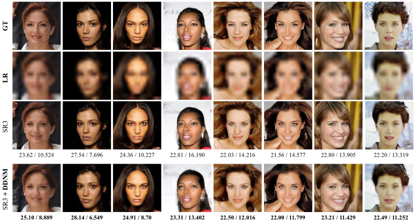
Figure 11: DDNM can be applied to SR3 to improve the restoration performance. Here we experiment on 8$\times$ SR (from image size 16$\times$16 to 128$\times$128), the metrics are PSNR/Consistency.

Algorithm 10 Reverse Diffusion Process of SDE (conditional)

Require: The condition $\mathbf{y}$, the operator $\mathbf{A}$ and the rate $\lambda$

1:$\mathbf{x}_{T}\sim\mathcal{N}(\mathbf{0},\mathbf{I})$.

2:for $t=T,...,1$ do

3:     $\bm{\epsilon}_{1},\bm{\epsilon}_{2}\sim\mathcal{N}(\mathbf{0},\mathbf{I})$ if $t>1$, else $\bm{\epsilon}_{1},\bm{\epsilon}_{2}=\mathbf{0}$.

4:     $\hat{\mathbf{x}}_{t}=\mathbf{x}_{t}+\lambda\nabla_{\mathbf{x}_{t}}f(\mathbf{A}\mathbf{x}_{t},\mathbf{y})$

5:     $\mathbf{x}_{t-1}=\frac{1}{\sqrt{\alpha}_{t}}\left({\color[rgb]{0,0,1}\hat{\mathbf{x}}_{t}}-\mathcal{Z}_{\bm{\theta}}({\color[rgb]{0,0,1}\hat{\mathbf{x}}_{t}},t)\frac{\beta_{t}}{\sqrt{1-\bar{\alpha}_{t}}}\right)+\sigma_{t}\bm{\epsilon}_{2}$

6:return $\mathbf{x}_{0}$

Song et al. (2020) propose a conditional sampling strategy in diffusion models, which we abbreviate as SDE in this paper. Specifically, SDE optimize each latent variable $\mathbf{x}_{t}$ toward a specific condition $f(\mathbf{A}\mathbf{x}_{t},\mathbf{y})$ and put the optimized $\mathbf{x}_{t}$ back to the original reverse diffusion process, as is shown in Algo. 10. $\mathbf{y}$ is the condition and $\mathbf{A}$ is an operator with $f(\cdot,\cdot)$ measures the distance between $\mathbf{A}\mathbf{x}_{t}$ and $\mathbf{y}$.

It is worth noting that DDNM is compatible with extra sources of constraints in the form of operation 5 in Algo. 10. For example, our results in Fig. 1 and Fig. 3 are generated using the diffusion model pretrained on ImageNet with classifier guidance.

Appendix I Solving noisy Image Restoration Precisely

For noisy tasks $\mathbf{y}=\mathbf{Ax+n},\mathbf{n}\sim\mathcal{N}(\mathbf{0},\sigma_{\mathbf{y}}^{2}\mathbf{I})$, Sec. 3.3 provide a simple solution where $\mathbf{A}^{\dagger}\mathbf{n}$ is approximated as $\mathcal{N}(\mathbf{0},\sigma_{\mathbf{y}}^{2}\mathbf{I})$. However, the precise distribution of $\mathbf{A}^{\dagger}\mathbf{n}$ is $\mathcal{N}(\mathbf{0},\sigma_{\mathbf{y}}^{2}\mathbf{A}^{\dagger}(\mathbf{A}^{\dagger})^{T})$ where the covariance matrix is usually non-diagonal. To use similar principles in Eq. 19, we need to orthodiagonalize this matrix. Next, we conduct detailed derivations.

This solution involves the Singular Value Decomposition(SVD), which can decompose the degradation operator $\mathbf{A}$ and yield its pseudo-inverse $\mathbf{A}^{\dagger}$:

$$\mathbf{A}=\mathbf{U\Sigma V}^{\top} ,\quad\mathbf{A}^{\dagger}=\mathbf{V\Sigma^{\dagger}U}^{\top},$$ (35)

$$\mathbf{A}\in\mathbb{R}^{d\times D},\mathbf{A}^{\dagger}\in\mathbb{R}^{D\times d},\mathbf{U}\in\mathbb{R}^{d\times d} ,\mathbf{V}\in\mathbb{R}^{D\times D},\mathbf{\Sigma}\in\mathbb{R}^{d\times D},\mathbf{\Sigma}^{\dagger}\in\mathbb{R}^{D\times d},$$ (36)

$$\mathbf{\Sigma}=diag\{s_{1},s_{2},\cdots,s_{d}\},\quad\mathbf{\Sigma}^{(i)} =s_{i},\quad\mathbf{\Sigma}^{\dagger(i)}=\begin{cases}\frac{1}{s_{i}},&s_{i}\neq 0,\\ 0,&s_{i}=0\end{cases},$$ (37)

To find out how much noise has been introduced into $\mathbf{\hat{x}}_{0|t}$, we first rewrite Eq. 17 as:

$$\mathbf{\hat{x}}_{0|t}=\mathbf{x}_{0|t}-\mathbf{\Sigma_{t}}\mathbf{A}^{\dagger}(\mathbf{A}\mathbf{x}_{0|t}-\mathbf{A}\mathbf{x}-\mathbf{n}),$$ (38)

where $\mathbf{A}\mathbf{x}$ represents the clean measurements before adding noise. $\mathbf{\Sigma_{t}}=\mathbf{V}\Lambda_{t}\mathbf{V}^{\top}$ is the scaling matrix with $\Lambda_{t}=diag\{\lambda_{t1},\lambda_{t2},\cdots,\lambda_{tD}\}$. Then we can rewrite the additive noise $\mathbf{n}$ as $\sigma_{\mathbf{y}}\bm{\epsilon}_{\mathbf{n}}$ where $\bm{\epsilon}_{\mathbf{n}}\sim\mathcal{N}(\mathbf{0},\mathbf{I})$. Now Eq. 38 becomes

$$\mathbf{\hat{x}}_{0|t}=\mathbf{x}_{0|t}-\mathbf{\Sigma}_{t}\mathbf{A}^{\dagger}(\mathbf{A}\mathbf{x}_{0|t}-\mathbf{A}\mathbf{x})+\sigma_{\mathbf{y}}\mathbf{V}\Lambda_{t}\mathbf{V}^{\top}\mathbf{A}^{\dagger}\bm{\epsilon}_{\mathbf{n}},$$ (39)

where $\mathbf{x}_{0|t}-\mathbf{\Sigma}_{t}\mathbf{A}^{\dagger}(\mathbf{A}\mathbf{x}_{0|t}-\mathbf{A}\mathbf{x})$ denotes the clean part of $\mathbf{\hat{x}}_{0|t}$ (written as $\mathbf{\hat{x}}_{0|t}^{c}$). It is clear that the noise introduced into $\mathbf{\hat{x}}_{0|t}$ is $\sigma_{\mathbf{y}}\mathbf{V}\Lambda_{t}\mathbf{V}^{\top}\mathbf{A}^{\dagger}\bm{\epsilon}_{\mathbf{n}}$. The handling of the introduced noise depends on the sampling strategy we used. We will discuss the solution for DDPM and DDIM, respectively.

The Situation in DDPM.

When using DDPM as the sampling strategy, we yield $\mathbf{x}_{t-1}$ by sampling from $p(\mathbf{x}_{t-1}|\mathbf{x}_{t},\mathbf{x}_{0})=\mathcal{N}(\mathbf{x}_{t-1};\mathbf{\mu}_{t}(\mathbf{x}_{t},\mathbf{x}_{0}),\sigma_{t}^{2}\mathbf{I})$, i.e.,

$$\mathbf{x}_{t-1}=\frac{\sqrt{\bar{\alpha}_{t-1}}\beta_{t}}{1-\bar{\alpha}_{t}}\hat{\mathbf{x}}_{0|t}+\frac{\sqrt{\alpha_{t}}(1-\bar{\alpha}_{t-1})}{1-\bar{\alpha}_{t}}\mathbf{x}_{t}+\sigma_{t}\bm{\epsilon},\quad\bm{\epsilon}\sim\mathcal{N}(\mathbf{0},\mathbf{I}),$$ (40)

Considering the introduced noise, we change $\sigma_{t}\bm{\epsilon}$ to ensure the entire noise level not exceed $\mathcal{N}(\mathbf{0},\sigma_{t}^{2}\mathbf{I})$. Hence we construct a new noise $\bm{\epsilon}_{new}\sim\mathcal{N}(\mathbf{0},\mathbf{\Phi}_{t}\mathbf{I})$. Then the Eq. 40 becomes

$$\mathbf{x}_{t-1}=\frac{\sqrt{\bar{\alpha}_{t-1}}\beta_{t}}{1-\bar{\alpha}_{t}}\hat{\mathbf{x}}^{c}_{0|t} +\frac{\sqrt{\alpha_{t}}(1-\bar{\alpha}_{t-1})}{1-\bar{\alpha}_{t}}\mathbf{x}_{t}+\bm{\epsilon}_{intro}+\bm{\epsilon}_{new},$$ (41)

$$\bm{\epsilon}_{intro} =\frac{\sqrt{\bar{\alpha}_{t-1}}\beta_{t}}{1-\bar{\alpha}_{t}}\sigma_{\mathbf{y}}\mathbf{V}\Lambda_{t}\mathbf{V}^{\top}\mathbf{A}^{\dagger}\bm{\epsilon}_{\mathbf{n}},$$ (42)

$$\bm{\epsilon}_{intro} +\bm{\epsilon}_{new}\sim\mathcal{N}(\mathbf{0},\sigma_{t}^{2}\mathbf{I}).$$ (43)

$\bm{\epsilon}_{intro}$ denotes the introduced noise, which can be further written as

$$\bm{\epsilon}_{intro} =\frac{\sqrt{\bar{\alpha}_{t-1}}\beta_{t}}{1-\bar{\alpha}_{t}}\sigma_{\mathbf{y}}\mathbf{V}\Lambda_{t}\mathbf{V}^{\top}\mathbf{A}^{\dagger}\bm{\epsilon}_{\mathbf{n}}$$ (44)

$$\sim\mathcal{N}(\mathbf{0},(\frac{\sqrt{\bar{\alpha}_{t-1}}\beta_{t}}{1-\bar{\alpha}_{t}})^{2}\sigma_{\mathbf{y}}^{2}(\mathbf{V}\Lambda_{t}\mathbf{V}^{\top}\mathbf{A}^{\dagger})\mathbf{I}(\mathbf{V}\Lambda_{t}\mathbf{V}^{\top}\mathbf{A}^{\dagger})^{\top})$$ (45)

$$\sim\mathcal{N}(\mathbf{0},(\frac{\sqrt{\bar{\alpha}_{t-1}}\beta_{t}}{1-\bar{\alpha}_{t}})^{2}\sigma_{\mathbf{y}}^{2}\mathbf{V}\Lambda_{t}\mathbf{V}^{\top}\mathbf{A}^{\dagger}(\mathbf{A}^{\dagger})^{\top}\mathbf{V}\Lambda_{t}\mathbf{V}^{\top})$$ (46)

$$\sim\mathcal{N}(\mathbf{0},(\frac{\sqrt{\bar{\alpha}_{t-1}}\beta_{t}}{1-\bar{\alpha}_{t}})^{2}\sigma_{\mathbf{y}}^{2}\mathbf{V}\Lambda_{t}\mathbf{V}^{\top}\mathbf{V}\mathbf{\Sigma}^{\dagger}\mathbf{U}^{\top}\mathbf{U}(\mathbf{\Sigma}^{\dagger})^{\top}\mathbf{V}^{\top}\mathbf{V}\Lambda_{t}\mathbf{V}^{\top})$$ (47)

$$\sim\mathcal{N}(\mathbf{0},(\frac{\sqrt{\bar{\alpha}_{t-1}}\beta_{t}}{1-\bar{\alpha}_{t}})^{2}\sigma_{\mathbf{y}}^{2}\mathbf{V}\Lambda_{t}\mathbf{\Sigma}^{\dagger}(\mathbf{\Sigma}^{\dagger})^{\top}\Lambda_{t}\mathbf{V}^{\top})$$ (48)

The variance matrix of $\bm{\epsilon}_{intro}$ can be simplified as $\mathbf{V}\mathbf{D}_{t}\mathbf{V}^{\top}$, with $\mathbf{D}_{t}=diag\{d_{t1},d_{t2},\cdots,d_{tD}\}$:

$$\bm{\epsilon}_{intro}\sim\mathcal{N}(\mathbf{0},\mathbf{V}\mathbf{D}_{t}\mathbf{V}^{\top}),\quad d_{ti}=\begin{cases}\frac{({\frac{\sqrt{\bar{\alpha}_{t-1}}\beta_{t}}{1-\bar{\alpha}_{t}}})^{2}\sigma_{\mathbf{y}}^{2}\lambda_{ti}^{2}}{s_{i}^{2}},&s_{i}\neq 0,\\ 0,&s_{i}=0\end{cases},$$ (49)

To construct $\bm{\epsilon}_{new}$, we define a new diagonal matrix $\mathbf{\Gamma}_{t}(=diag\{\gamma_{t1},\gamma_{t2},\cdots,\gamma_{tD}\})$:

$$\mathbf{\Gamma}_{t}=\sigma_{t}^{2}\mathbf{I}-\mathbf{D}_{t},\quad\gamma_{ti}=\begin{cases}\sigma_{t}^{2}-\frac{({\frac{\sqrt{\bar{\alpha}_{t-1}}\beta_{t}}{1-\bar{\alpha}_{t}}})^{2}\sigma_{\mathbf{y}}^{2}\lambda_{ti}^{2}}{s_{i}^{2}},&s_{i}\neq 0,\\ \sigma_{t}^{2},&s_{i}=0\end{cases},$$ (50)

Now we can yield $\bm{\epsilon}_{new}$ by sampling from $\mathcal{N}(\mathbf{0},\mathbf{V}\mathbf{\Gamma}_{t}\mathbf{V}^{\top})$ to ensure that $\bm{\epsilon}_{intro}+\bm{\epsilon}_{new}\sim\mathcal{N}(\mathbf{0},\mathbf{V}(\mathbf{D}_{t}+\mathbf{\Gamma}_{t})\mathbf{V}^{\top})=\mathcal{N}(\mathbf{0},\sigma_{t}^{2}\mathbf{I})$. An easier implementation method is firstly sampling $\bm{\epsilon}_{temp}$ from $\mathcal{N}(\mathbf{0},\mathbf{\Gamma}_{t})$ and finally get $\bm{\epsilon}_{new}=\mathbf{V}\bm{\epsilon}_{temp}.$ From Eq. 50, we also observe that $\lambda_{ti}$ guarantees the noise level of the introduced noise do not exceed the pre-defined noise level $\sigma_{t}$ so that we can get the formula of $\lambda_{ti}$ in $\mathbf{\Sigma}_{t}(=\mathbf{V}\Lambda_{t}\mathbf{V}^{\top},\Lambda_{t}=diag\{\lambda_{t1},\lambda_{t2},\cdots,\lambda_{tD}\}\})$:

$$\lambda_{ti} =\begin{cases}1,&\sigma_{t}\geq\frac{({\frac{\sqrt{\bar{\alpha}_{t-1}}\beta_{t}}{1-\bar{\alpha}_{t}}})\sigma_{\mathbf{y}}}{s_{i}}\\ \frac{\sigma_{t}s_{i}}{({\frac{\sqrt{\bar{\alpha}_{t-1}}\beta_{t}}{1-\bar{\alpha}_{t}}})\sigma_{\mathbf{y}}},&\sigma_{t}<\frac{({\frac{\sqrt{\bar{\alpha}_{t-1}}\beta_{t}}{1-\bar{\alpha}_{t}}})\sigma_{\mathbf{y}}}{s_{i}}\\ 1,&s_{i}=0\end{cases},$$ (51)

The Situation in DDIM.

When using DDIM as the sampling strategy, the process of getting $\mathbf{x}_{t-1}$ from $\mathbf{x}_{t}$ becomes:

$$\mathbf{x}_{t-1}=\sqrt{\bar{\alpha}_{t-1}}\mathbf{\hat{x}}_{0|t}+\sigma_{t}\sqrt{1-\eta^{2}}\mathcal{Z}_{\bm{\theta}}(\mathbf{x}_{t},t)+\sigma_{t}\eta\bm{\epsilon},\quad\bm{\epsilon}\sim\mathcal{N}(\mathbf{0},\mathbf{I}),$$ (52)

where $\sigma_{t}=\sqrt{1-\bar{\alpha}_{t-1}}$ is the noise level of the $t$-th time-step, $\mathcal{Z}_{\bm{\theta}}$ is the denoiser which estimates the additive noise from $\mathbf{x}_{t}$ and $\eta$ control the randomness of this sampling process. Considering the noise part is subject to a normal distribution, that is, $\sigma_{t}\sqrt{1-\eta^{2}}\mathcal{Z}_{\bm{\theta}}(\mathbf{x}_{t},t)+\sigma_{t}\eta\bm{\epsilon}\sim\mathcal{N}(\mathbf{0},\sigma_{t}^{2}\mathbf{I})$, so that the equation can be rewritten as

$$\mathbf{x}_{t-1}=\sqrt{\bar{\alpha}_{t-1}}\mathbf{\hat{x}}_{0|t}+\bm{\epsilon}_{orig},\quad\bm{\epsilon}_{orig}\sim\mathcal{N}(\mathbf{0},\sigma_{t}^{2}\mathbf{I})$$ (53)

Considering the introduced noise, we change $\bm{\epsilon}_{orig}$ to ensure the entire noise level not exceed $\mathcal{N}(\mathbf{0},\sigma_{t}^{2}\mathbf{I})$. Hence we construct a new noise term $\bm{\epsilon}_{new}\sim\mathcal{N}(\mathbf{0},\mathbf{\Phi}_{t}\mathbf{I})$:

$$\mathbf{x}_{t-1}=\sqrt{\bar{\alpha}_{t-1}}\mathbf{\hat{x}}_{0|t}^{c}+\bm{\epsilon}_{intro}+\bm{\epsilon}_{new},$$ (54)

$$\bm{\epsilon}_{intro}=\sqrt{\bar{\alpha}_{t-1}}\sigma_{\mathbf{y}}\mathbf{V}\Lambda_{t}\mathbf{V}^{\top}\mathbf{A}^{\dagger}\bm{\epsilon}_{\mathbf{n}},$$ (55)

$$\bm{\epsilon}_{intro}+\bm{\epsilon}_{new}\sim\mathcal{N}(\mathbf{0},\sigma_{t}^{2}\mathbf{I}).$$ (56)

$\bm{\epsilon}_{intro}$ denotes the introduced noise, which can be further written as

$$\bm{\epsilon}_{intro} =\sqrt{\bar{\alpha}_{t-1}}\sigma_{\mathbf{y}}\mathbf{V}\Lambda_{t}\mathbf{V}^{\top}\mathbf{A}^{\dagger}\bm{\epsilon}_{\mathbf{n}}$$ (57)

$$\sim\mathcal{N}(\mathbf{0},\bar{\alpha}_{t-1}\sigma_{\mathbf{y}}^{2}(\mathbf{V}\Lambda_{t}\mathbf{V}^{\top}\mathbf{A}^{\dagger})\mathbf{I}(\mathbf{V}\Lambda_{t}\mathbf{V}^{\top}\mathbf{A}^{\dagger})^{\top})$$ (58)

$$\sim\mathcal{N}(\mathbf{0},\bar{\alpha}_{t-1}\sigma_{\mathbf{y}}^{2}\mathbf{V}\Lambda_{t}\mathbf{V}^{\top}\mathbf{A}^{\dagger}(\mathbf{A}^{\dagger})^{\top}\mathbf{V}\Lambda_{t}\mathbf{V}^{\top})$$ (59)

$$\sim\mathcal{N}(\mathbf{0},\bar{\alpha}_{t-1}\sigma_{\mathbf{y}}^{2}\mathbf{V}\Lambda_{t}\mathbf{V}^{\top}\mathbf{V}\mathbf{\Sigma}^{\dagger}\mathbf{U}^{\top}\mathbf{U}(\mathbf{\Sigma}^{\dagger})^{\top}\mathbf{V}^{\top}\mathbf{V}\Lambda_{t}\mathbf{V}^{\top})$$ (60)

$$\sim\mathcal{N}(\mathbf{0},\bar{\alpha}_{t-1}\sigma_{\mathbf{y}}^{2}\mathbf{V}\Lambda_{t}\mathbf{\Sigma}^{\dagger}(\mathbf{\Sigma}^{\dagger})^{\top}\Lambda_{t}\mathbf{V}^{\top})$$ (61)

The variance matrix of $\bm{\epsilon}_{intro}$ can be simplified as $\mathbf{V}\mathbf{D}_{t}\mathbf{V}^{\top}$, with $\mathbf{D}_{t}=diag\{d_{t1},d_{t2},\cdots,d_{tD}\}$:

$$\bm{\epsilon}_{intro}\sim\mathcal{N}(\mathbf{0},\mathbf{V}\mathbf{D}_{t}\mathbf{V}^{\top}),\quad d_{ti}=\begin{cases}\frac{\bar{\alpha}_{t-1}\sigma_{\mathbf{y}}^{2}\lambda_{ti}^{2}}{s_{i}^{2}},&s_{i}\neq 0,\\ 0,&s_{i}=0\end{cases},$$ (62)

To construct $\bm{\epsilon}_{new}$, we define a new diagonal matrix $\mathbf{\Gamma}_{t}(=diag\{\gamma_{t1},\gamma_{t2},\cdots,\gamma_{tD}\})$:

$$\mathbf{\Gamma}_{t}=\sigma_{t}^{2}\mathbf{I}-\mathbf{D}_{t},\quad\gamma_{ti}=\begin{cases}\sigma_{t}^{2}-\frac{\bar{\alpha}_{t-1}\sigma_{\mathbf{y}}^{2}\lambda_{ti}^{2}}{s_{i}^{2}},&s_{i}\neq 0,\\ \sigma_{t}^{2},&s_{i}=0\end{cases},$$ (63)

Now we can construct $\bm{\epsilon}_{new}$ by sampling from $\mathcal{N}(\mathbf{0},\mathbf{V}\mathbf{\Gamma}_{t}\mathbf{V}^{\top})$ to ensure that $\bm{\epsilon}_{intro}+\bm{\epsilon}_{new}\sim\mathcal{N}(\mathbf{0},\mathbf{V}(\mathbf{D}_{t}+\mathbf{\Gamma}_{t})\mathbf{V}^{\top})=\mathcal{N}(\mathbf{0},\sigma_{t}^{2}\mathbf{I})$. An easier implementation is firstly sampling $\bm{\epsilon}_{temp}$ from $\mathcal{N}(\mathbf{0},\mathbf{\Gamma}_{t})$ and finally get $\bm{\epsilon}_{new}=\mathbf{V}\bm{\epsilon}_{temp}.$ From Eq. 63, we also observe that $\lambda_{ti}$ guarantees the noise level of the introduced noise do not exceed the pre-defined noise level $\sigma_{t}$ so that we can get the formula of $\lambda_{ti}$ in $\mathbf{\Sigma}_{t}(=\mathbf{V}\Lambda_{t}\mathbf{V}^{\top},\Lambda_{t}=diag\{\lambda_{t1},\lambda_{t2},\cdots,\lambda_{tD}\}\})$:

$$\lambda_{ti}=\begin{cases}1,&\sigma_{t}\geq\frac{\sqrt{\bar{\alpha}_{t-1}}\sigma_{\mathbf{y}}}{s_{i}},\\ \frac{s_{i}\sigma_{t}{\color[rgb]{0,0,1}\sqrt{1-\eta^{2}}}}{\sqrt{\bar{\alpha}_{t-1}}\sigma_{\mathbf{y}}},&\sigma_{t}<\frac{\sqrt{\bar{\alpha}_{t-1}}\sigma_{\mathbf{y}}}{s_{i}},\\ 1,&s_{i}=0,\end{cases},$$ (64)

In the actual implementation, we have adopted the following formula for $\bm{\epsilon}_{temp}$ and it can be proved that its distribution is $\mathcal{N}(\mathbf{0},\mathbf{\Gamma}_{t})$:

$$\bm{\epsilon}_{temp}^{(i)}=\begin{cases}\sqrt{\sigma_{t}^{2}-\frac{\bar{\alpha}_{t-1}\sigma_{\mathbf{y}}^{2}}{s_{i}^{2}}}\bm{\epsilon}^{(i)},&\sigma_{t}\geq\frac{\sqrt{\bar{\alpha}_{t-1}}\sigma_{\mathbf{y}}}{s_{i}},\\ \sigma_{t}{\color[rgb]{0,0,1}\eta}\bm{\epsilon}^{(i)},&\sigma_{t}<\frac{\sqrt{\bar{\alpha}_{t-1}}\sigma_{\mathbf{y}}}{s_{i}},\\ \sigma_{t}\sqrt{1-\eta^{2}}\mathcal{Z}_{\bm{\theta}}^{(i)}+\sigma_{t}\eta\bm{\epsilon}^{(i)},&s_{i}=0,\end{cases},$$ (65)

where $\bm{\epsilon}_{temp}^{(i)}$ denotes the $i$-th element of the vector $\bm{\epsilon}_{temp}$ and $\bm{\epsilon}\sim\mathcal{N}(\mathbf{0},\mathbf{I})$.

Note that the blue ${\color[rgb]{0,0,1}\eta}$ is not necessarily needed. By our theory in Sec. 3.3, ${\color[rgb]{0,0,1}\eta}$ should be 0 to maximize the preservation of range-space correction. But inspired by DDRM(Kawar et al., 2022), we find that involving ${\color[rgb]{0,0,1}\eta}$ help improves the robustness, though sacrificing some range-space information.

Appendix J Additional Results

We present additional quantitative results in Tab. 5, with corresponding visual results of DDNM in Fig. 12 and Fig. 13. Additional visual results of DDNM⁺ are shown in Fig. 14 and Fig. 15. Additional results for real-world photo restoration are presented in Fig. 16. Note that all the additional results presented here do not use the time-travel trick.

CelebA-HQ	4$\times$ bicubic SR				8$\times$ bicubic SR				16$\times$ bicubic SR
Method	PSNR↑	SSIM↑	Cons↓	FID↓	PSNR↑	SSIM↑	Cons↓	FID↓	PSNR↑	SSIM↑	Cons↓	FID↓
DDRM	31.63	0.9452	33.88	31.04	28.11	0.9039	3.23	38.84	24.80	0.8612	0.36	46.67
DDNM	31.63	0.9450	4.80	22.27	28.18	0.9043	0.68	37.50	24.96	0.8634	0.10	45.5
ImageNet	4$\times$ bicubic SR				8$\times$ bicubic SR				16$\times$ bicubic SR
Method	PSNR↑	SSIM↑	Cons↓	FID↓	PSNR↑	SSIM↑	Cons↓	FID↓	PSNR↑	SSIM↑	Cons↓	FID↓
DDRM	27.38	0.8698	19.79	43.15	23.75	0.7668	2.70	83.67	20.85	0.6842	0.38	130.81
DDNM	27.46	0.8707	4.92	39.26	23.79	0.7684	0.72	80.15	20.90	0.6853	0.11	128.13
CelebA-HQ	inpainting (Mask 1)				inpainting (Mask 2)				inpainting (Mask 3)
Method	PSNR↑	SSIM↑	Cons↓	FID↓	PSNR↑	SSIM↑	Cons↓	FID↓	PSNR↑	SSIM↑	Cons↓	FID↓
DDRM	34.79	0.9783	1325.46	12.53	38.27	0.9879	1357.09	10.34	35.77	0.9767	-	21.49
DDNM	35.64	0.9823	0.0	4.54	39.38	0.9915	0.0	2.82	36.32	0.9797	-	12.46
ImageNet	inpainting (Mask 1)				inpainting (Mask 2)				inpainting (Mask 3)
Method	PSNR↑	SSIM↑	Cons↓	FID↓	PSNR↑	SSIM↑	Cons↓	FID↓	PSNR↑	SSIM↑	Cons↓	FID↓
DDRM	31.73	0.9663	876.86	4.82	34.60	0.9785	1036.85	3.77	31.34	0.9439	-	12.84
DDNM	32.06	0.9682	0.0	3.89	34.92	0.9801	0.0	3.19	31.62	0.9461	-	9.73
CelebA-HQ	deblur (Gaussian)				deblur (anisotropic)				deblur (uniform)
Method	PSNR↑	SSIM↑	Cons↓	FID↓	PSNR↑	SSIM↑	Cons↓	FID↓	PSNR↑	SSIM↑	Cons↓	FID↓
DDRM	43.07	0.9937	297.15	6.24	41.29	0.9909	312.14	7.02	40.95	0.9900	182.27	7.74
DDNM	46.72	0.9966	60.00	1.41	43.19	0.9931	66.14	2.80	42.85	0.9923	41.86	3.79
ImageNet	deblur (Gaussian)				deblur (anisotropic)				deblur (uniform)
Method	PSNR↑	SSIM↑	Cons↓	FID↓	PSNR↑	SSIM↑	Cons↓	FID↓	PSNR↑	SSIM↑	Cons↓	FID↓
DDRM	43.01	0.9921	207.90	1.48	40.01	0.9855	221.23	2.55	39.72	0.9829	134.60	3.73
DDNM	44.93	0.9937	59.09	1.15	40.81	0.9864	63.89	2.14	40.70	0.9844	41.86	3.22

CelebA-HQ	CS (ratio=0.5)				CS (ratio=0.25)
Method	PSNR↑	SSIM↑	Cons↓	FID↓	PSNR↑	SSIM↑	Cons↓	FID↓
DDRM	31.52	0.9520	2171.76	25.71	24.86	0.8765	1869.03	46.77
DDNM	33.44	0.9604	1640.67	15.81	27.56	0.9090	1511.51	28.80
ImageNet	CS (ratio=0.5)				CS (ratio=0.25)
Method	PSNR↑	SSIM↑	Cons↓	FID↓	PSNR↑	SSIM↑	Cons↓	FID↓
DDRM	26.94	0.8902	6293.69	25.01	19.95	0.7048	3444.50	97.99
DDNM	29.22	0.9106	5564.00	18.55	21.66	0.7493	3162.30	64.68

CelebA-HQ	Colorization
Method	PSNR↑	SSIM↑	Cons↓	FID↓
DDRM	26.38	0.7974	455.90	31.26
DDNM	26.25	0.7947	48.87	26.44
ImageNet	Colorization
Method	PSNR↑	SSIM↑	Cons↓	FID↓
DDRM	23.34	0.6429	260.43	36.56
DDNM	23.47	0.6550	42.32	36.32

Table 5: Comprehensive quantitative comparisons between DDNM and DDRM.

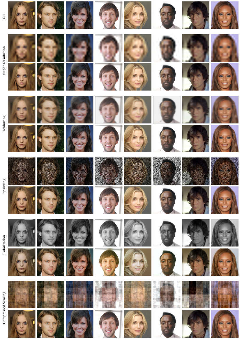
Figure 12: Image restoration results of DDNM on CelebA.

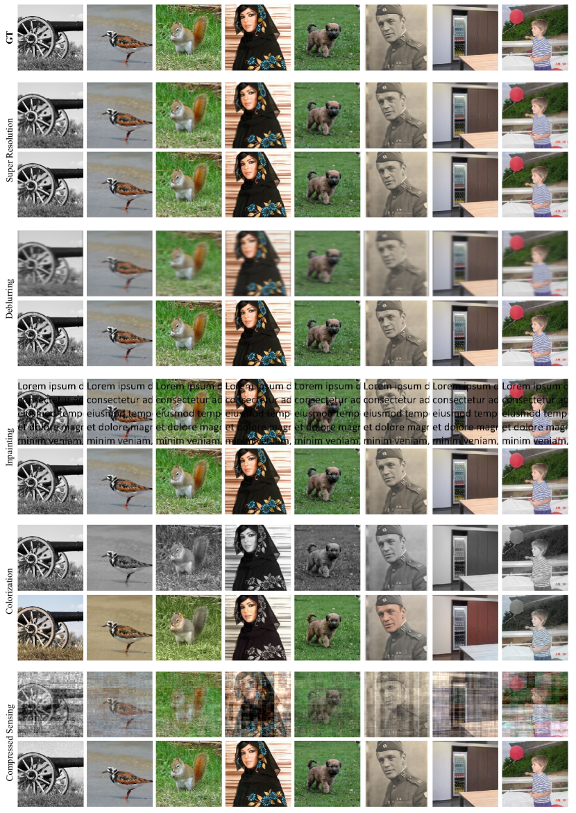
Figure 13: Image restoration results of DDNM on ImageNet.

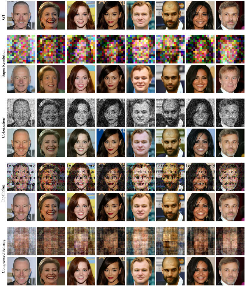
Figure 14: Noisy image restoration results of DDNM⁺ on CelebA. The results here do not use the time-travel trick.

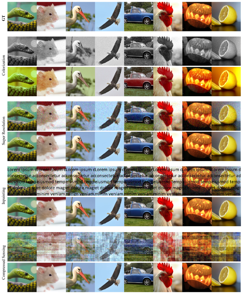
Figure 15: Noisy image restoration results of DDNM⁺ on ImageNet. The results here do not use the time-travel trick.

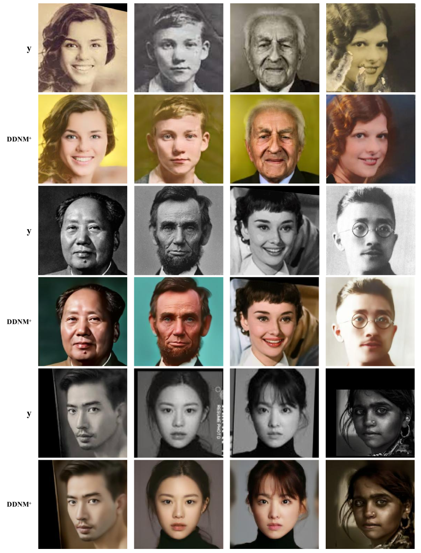
Figure 16: Restoring real-world photos using DDNM. $\mathbf{y}$ represents the degraded images collected from the internet. The results here do not use the time-travel trick.

References

- Agustsson & Timofte (2017) Eirikur Agustsson and Radu Timofte. Ntire 2017 challenge on single image super-resolution: Dataset and study. In 2017 IEEE Conference on Computer Vision and Pattern Recognition Workshops (CVPRW), 2017.
- Andrews & Hunt (1977) Harry C Andrews and Boby Ray Hunt. Digital image restoration. 1977.
- Bahat & Michaeli (2014) Yuval Bahat and Tomer Michaeli. Auto-encoding variational bayes. In In The International Conference on Learning Representations (ICLR), 2014.
- Bahat & Michaeli (2020) Yuval Bahat and Tomer Michaeli. Explorable super resolution. In Proceedings of the IEEE/CVF Conference on Computer Vision and Pattern Recognition (CVPR), 2020.
- Chan et al. (2021) Kelvin CK Chan, Xintao Wang, Xiangyu Xu, Jinwei Gu, and Chen Change Loy. Glean: Generative latent bank for large-factor image super-resolution. In Proceedings of the IEEE/CVF Conference on Computer Vision and Pattern Recognition (CVPR), 2021.
- Chen & Davies (2020) Dongdong Chen and Mike E Davies. Deep decomposition learning for inverse imaging problems. In European Conference on Computer Vision (ECCV). Springer, 2020.
- Choi et al. (2021) Jooyoung Choi, Sungwon Kim, Yonghyun Jeong, Youngjune Gwon, and Sungroh Yoon. Ilvr: Conditioning method for denoising diffusion probabilistic models. In Proceedings of the IEEE/CVF International Conference on Computer Vision (ICCV), 2021.
- Chung et al. (2022a) Hyungjin Chung, Jeongsol Kim, Michael T Mccann, Marc L Klasky, and Jong Chul Ye. Diffusion posterior sampling for general noisy inverse problems. arXiv preprint arXiv:2209.14687, 2022a.
- Chung et al. (2022b) Hyungjin Chung, Byeongsu Sim, and Jong Chul Ye. Improving diffusion models for inverse problems using manifold constraints. In Advances in Neural Information Processing Systems (NeurIPS), 2022b.
- Dhariwal & Nichol (2021) Prafulla Dhariwal and Alexander Nichol. Diffusion models beat gans on image synthesis. Advances in Neural Information Processing Systems (NeurIPS), 34, 2021.
- Dong et al. (2015) Chao Dong, Chen Change Loy, Kaiming He, and Xiaoou Tang. Image super-resolution using deep convolutional networks. IEEE Transactions on Pattern Analysis and Machine Intelligence, 38, 2015.
- Goodfellow et al. (2014) Ian Goodfellow, Jean Pouget-Abadie, Mehdi Mirza, Bing Xu, David Warde-Farley, Sherjil Ozair, Aaron Courville, and Yoshua Bengio. Generative adversarial nets. Advances in Neural Information Processing Systems (NeurIPS), 2014.
- Heusel et al. (2017) Martin Heusel, Hubert Ramsauer, Thomas Unterthiner, Bernhard Nessler, and Sepp Hochreiter. Gans trained by a two time-scale update rule converge to a local nash equilibrium. Advances in Neural Information Processing Systems (NeurIPS), 30, 2017.
- Ho et al. (2020) Jonathan Ho, Ajay Jain, and Pieter Abbeel. Denoising diffusion probabilistic models. Advances in Neural Information Processing Systems (NeurIPS), 33, 2020.
- Ho et al. (2022) Jonathan Ho, Tim Salimans, Alexey A Gritsenko, William Chan, Mohammad Norouzi, and David J Fleet. Video diffusion models. In ICLR Workshop on Deep Generative Models for Highly Structured Data, 2022.
- Karras et al. (2019) Tero Karras, Samuli Laine, and Timo Aila. A style-based generator architecture for generative adversarial networks. In Proceedings of the IEEE/CVF Conference on Computer Vision and Pattern Recognition (CVPR), 2019.
- Karras et al. (2020) Tero Karras, Samuli Laine, Miika Aittala, Janne Hellsten, Jaakko Lehtinen, and Timo Aila. Analyzing and improving the image quality of stylegan. In Proceedings of the IEEE/CVF Conference on Computer Vision and Pattern Recognition (CVPR), 2020.
- Karras et al. (2021) Tero Karras, Miika Aittala, Samuli Laine, Erik Härkönen, Janne Hellsten, Jaakko Lehtinen, and Timo Aila. Alias-free generative adversarial networks. Advances in Neural Information Processing Systems (NeurIPS), 34, 2021.
- Kawar et al. (2022) Bahjat Kawar, Michael Elad, Stefano Ermon, and Jiaming Song. Denoising diffusion restoration models. In ICLR Workshop on Deep Generative Models for Highly Structured Data (ICLRW), 2022.
- Liang et al. (2021) Jingyun Liang, Jiezhang Cao, Guolei Sun, Kai Zhang, Luc Van Gool, and Radu Timofte. Swinir: Image restoration using swin transformer. In Proceedings of the IEEE/CVF International Conference on Computer Vision Workshops (ICCVW), 2021.
- Lugmayr et al. (2022) Andreas Lugmayr, Martin Danelljan, Andres Romero, Fisher Yu, Radu Timofte, and Luc Van Gool. Repaint: Inpainting using denoising diffusion probabilistic models. In Proceedings of the IEEE/CVF Conference on Computer Vision and Pattern Recognition (CVPR), 2022.
- Menon et al. (2020) Sachit Menon, Alexandru Damian, Shijia Hu, Nikhil Ravi, and Cynthia Rudin. Pulse: Self-supervised photo upsampling via latent space exploration of generative models. In Proceedings of the IEEE/CVF Conference on Computer Vision and Pattern Recognition (CVPR), 2020.
- Pan et al. (2021) Xingang Pan, Xiaohang Zhan, Bo Dai, Dahua Lin, Chen Change Loy, and Ping Luo. Exploiting deep generative prior for versatile image restoration and manipulation. IEEE Transactions on Pattern Analysis and Machine Intelligence, 2021.
- Richardson (1972) William Hadley Richardson. Bayesian-based iterative method of image restoration. JoSA, 62(1), 1972.
- Saharia et al. (2021) Chitwan Saharia, Jonathan Ho, William Chan, Tim Salimans, David J Fleet, and Mohammad Norouzi. Image super-resolution via iterative refinement. arXiv preprint arXiv:2104.07636, 2021.
- Saharia et al. (2022) Chitwan Saharia, William Chan, Huiwen Chang, Chris Lee, Jonathan Ho, Tim Salimans, David Fleet, and Mohammad Norouzi. Palette: Image-to-image diffusion models. In ACM SIGGRAPH 2022 Conference Proceedings, 2022.
- Schwab et al. (2019) Johannes Schwab, Stephan Antholzer, and Markus Haltmeier. Deep null space learning for inverse problems: convergence analysis and rates. Inverse Problems, 35(2), 2019.
- Song et al. (2021a) Jiaming Song, Chenlin Meng, and Stefano Ermon. Denoising diffusion implicit models. In International Conference on Learning Representations (ICLR), 2021a.
- Song & Ermon (2019) Yang Song and Stefano Ermon. Generative modeling by estimating gradients of the data distribution. Advances in Neural Information Processing Systems (NeurIPS), 32, 2019.
- Song et al. (2020) Yang Song, Jascha Sohl-Dickstein, Diederik P Kingma, Abhishek Kumar, Stefano Ermon, and Ben Poole. Score-based generative modeling through stochastic differential equations. In International Conference on Learning Representations (ICLR), 2020.
- Song et al. (2021b) Yang Song, Liyue Shen, Lei Xing, and Stefano Ermon. Solving inverse problems in medical imaging with score-based generative models. In International Conference on Learning Representations (ICLR), 2021b.
- Van Den Oord et al. (2017) Aaron Van Den Oord, Oriol Vinyals, et al. Neural discrete representation learning. Advances in Neural Information Processing Systems (NeurIPS), 30, 2017.
- Wang et al. (2021) Xintao Wang, Yu Li, Honglun Zhang, and Ying Shan. Towards real-world blind face restoration with generative facial prior. In Proceedings of the IEEE/CVF Conference on Computer Vision and Pattern Recognition (CVPR), 2021.
- Wang et al. (2022a) Yinhuai Wang, Yujie Hu, Jiwen Yu, and Jian Zhang. Gan prior based null-space learning for consistent super-resolution. arXiv preprint arXiv:2211.13524, 2022a.
- Wang et al. (2022b) Yinhuai Wang, Yujie Hu, and Jian Zhang. Panini-net: Gan prior based degradation-aware feature interpolation for face restoration. In Proceedings of the AAAI Conference on Artificial Intelligence (AAAI), 2022b.
- Whang et al. (2022) Jay Whang, Mauricio Delbracio, Hossein Talebi, Chitwan Saharia, Alexandros G Dimakis, and Peyman Milanfar. Deblurring via stochastic refinement. In Proceedings of the IEEE/CVF Conference on Computer Vision and Pattern Recognition (CVPR), 2022.
- Yang et al. (2021) Tao Yang, Peiran Ren, Xuansong Xie, and Lei Zhang. Gan prior embedded network for blind face restoration in the wild. In Proceedings of the IEEE/CVF Conference on Computer Vision and Pattern Recognition (CVPR), 2021.
- Zhang & Ghanem (2018) Jian Zhang and Bernard Ghanem. Ista-net: Interpretable optimization-inspired deep network for image compressive sensing. In Proceedings of the IEEE conference on computer vision and pattern recognition (CVPR), 2018.
- Zhang et al. (2020) Kai Zhang, Gool Luc-Van, and Timofte Radu. Deep unfolding network for image super-resolution. In Proceedings of the IEEE/CVF Conference on Computer Vision and Pattern Recognition (CVPR), 2020.
- Zhang et al. (2021) Kai Zhang, Jingyun Liang, Luc Van Gool, and Radu Timofte. Designing a practical degradation model for deep blind image super-resolution. In Proceedings of the IEEE/CVF International Conference on Computer Vision (ICCV), 2021.