Real-Time High-Quality Stereo Matching System on a GPU

Abstract

In this paper, we propose a low error rate and real-time stereo vision system on GPU. Many stereo vision systems on GPU have been proposed to date. In those systems, the error rates and the processing speed are in trade-off relationship. We propose a real-time stereo vision system on GPU for the high resolution images. This system also maintains a low error rate compared to other fast systems. In our approach, we have implemented the cost aggregation (CA), cross-checking and median filter on GPU in order to realize the real-time processing. Its processing speed is 40 fps for $1436\times{992}$ pixels images when the maximum disparity is 145, and its error rate is the lowest among the GPU systems which are faster than 30 fps.

I Introduction

The aim of stereo vision systems is to reconstruct the 3-D geometry of a scene from images taken by two separate cameras. The computational complexity of the stereo vision is very high, and many acceleration systems with GPUs, FPGAs and dedicated hardware have been developed [1][4]. All of them succeeded in real-time processing of high resolution images, but their accuracy is not good enough because they simplify the algorithms to fit the hardware architecture. In this paper, we aim to construct a real-time GPU stereo vision system for the high resolution image set ($1436\times{992}\times{145}$ disparities) in the Middlebury Benchmark.

GPUs have more than hundred cores which run faster than 1GHz, and drastic performance gain can be expected in many applications. However, the processing speed of the stereo vision by GPUs is much slower than FPGAs such as [2][3]. This is caused by the fact that data for several lines are intensively accessed at a time in the stereo vision, but the shared memory is too small to cache those lines. Therefore, many memory accesses to the global memory are required, and they limit the processing speed by GPUs. On the other hand, more sophisticated algorithms can be implemented on GPUs than FPGAs, and lower error rates have been achieved by many GPU systems[5][6]. The algorithms for the stereo vision can be categorized into two groups: local and global. In the local algorithms, only the local information around the target pixel is used to decide the disparity of the pixel, while the disparities of all pixels are decided considering the mutual effect of all pixels in the global algorithms. Thus, in general, the global algorithms achieve lower error rates, but require longer computation time. On many GPUs, algorithms which require only local information in each step, but propagate the mutual effect gradually by repeating the step many times are implemented. Their error rates are low enough, but their processing speed is far behind of the real-time requirement.

We have implemented a local search algorithm, which is an improved version of the algorithm that we have implemented on FPGA[9]. In our algorithm, AD (absolute difference) and mini-Census transform [14] are used to calculate the matching costs of the pixels in the two images, and they are aggregated along the $x$- and $y$-axes by using the Cross-based method [15][16], in order to compare the pixels as a block of the similar color. The matching costs are calculated twice using left and right image as the base, and two disparity maps are generated. Then, the disparity map is improved using the disparities which are common in both disparity maps. These operations are chosen to realize low error rates without repetitive computation. However, when we consider processing a high resolution image, its computational complexity is too high to achieve real-time processing. In order to achieve high performance, in this paper, we scale down the images to reduce the computational complexity. As shown in Fig.1, to reduce the computational complexity, we scale down the input images into a small size, and then scale up the disparity map to the original size. The images are scaled down to 1/4 by reducing the width and height by half, and the disparities are calculated on the scaled down images. The maximum disparity is also reduced to half, which means that the total computational complexity can be reduced to 1/8. This approach typically worsens the matching accuracy, but in our approach, an bilateral interpolation method is performed during the scaling up step, and a high matching accuracy can be maintained. This approach becomes possible because of the high quality of the high resolution images.

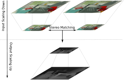
Figure 1: Image Scaling

II STEREO VISION

In the stereo vision systems, the matching of pixels in the two images (left and right) taken by two separate cameras is searched to reconstruct the 3-D geometry of the scene. When the two cameras are calibrated properly, epipolar restriction can be used. Under this restriction, we can obtain a disparity map $D_{map}$ by finding the matching of pixels on the epipolar lines of the two images as shown in Fig.2. Fig.2 shows how to calculate a disparity map using the left image as the base. A pixel in the left image $L(x,y)$ (or a window centered by $L(x,y)$) is compared with $D$ pixels $R(x-d,y)d=[0,D-1]$ in the right image (or $D$ windows centered by those pixels), and the most similar pixel to $L(x,y)$ is searched. $D$ is the maximum disparity value. Suppose that $R(x-d,y)$ is the most similar to $L(x,y)$. Then, this means that $L(x,y)$ and $R(x-d,y)$ are the same point of an object, and the distance $Z$ to the object can be calculated from d and two parameters of the two cameras using the following equation:

$$Z=f{\frac{B}{d}}.$$ (1)

Here, $f$ is the focus length of both cameras, and $B$ is the distance between the two cameras. Smaller d means that the object is farther away from the cameras, and $d=0$ means that the object is at infinity. The main problem in the stereo vision is to find the matching pixels in the two images correctly.

Another important problem in the stereo vision is the occlusion. When an object is taken by two cameras, some parts of the object appear in one image but do not appear in another image, depending on the positions and angles between the cameras and the object. These occlusions are the major source of errors in the stereo vision systems. In order to avoid those errors, $D_{map}$ is calculated twice: once using $L$, the left image, as the base ($D^{L}_{map}$), and another using $R$, the right image, as the base ($D^{R}_{map}$). Then, by using the same matching found in both $D^{L}_{map}$ and $D^{R}_{map}$ as the reliable disparities (called the ground control points, or GCPs), higher quality disparity maps can be obtained.

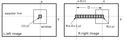
Figure 2: Local matching under the epipolar restriction

III OUR ALGORITHM

In this section, we introduce the details of our algorithm. Our algorithm consists of the following steps.

1. the two input images are gray-scaled

2. scaling down the two images

3. calculating matching cost of each pixel

4. cost aggregation along the $x$- and $y$-axes

5. generating two disparity maps

6. detecting GCPs (ground control pixels) by cross-checking the two disparity maps

7. refinement by a median filter and filling the non-GCPs by using a bilateral estimation method

8. scaling up the disparity map

III-A Scaling Down

In order to reduce the computational complexity, the two images are scaled down linearly in both horizontal and vertical directions using the mean-pooling method. Here, take the left image as an example:

$$L(x,y)=$$

$$\frac{1}{(2m+1)^{2}}\times{\sum_{j=-m}^{m}\sum_{i=-m}^{m}L_{org}(K\cdot{x}+i,K\cdot{y}+j)}$$ (2)

where $L_{org}(K\cdot{x}+i,K\cdot{y}+j)$ is the pixel in the original image, and $K$ is the factor for the scaling down (in our implementation, $K=2$). $L(x,y)$ is the pixel of the left scaled down image, and is smoothed by a mean-filter the size of which is $(2m+1)^{2}$. By choosing the block size carefully, we can avoid the loss of the matching accuracy, and can improve the processing speed.

III-B Matching cost between two pixels

The matching cost of each pixel is calculated using the absolute difference of the brightness and the mini-census transform. When the left image $L(x,y)$ is used as the base, the matching cost of the disparity $=d$ is given by

$$C^{L}(x,y,d)=C^{L}_{AD}(x,y,d)+C^{L}_{MC}(x,y,d).$$ (3)

$C^{L}_{AD}(x,y,d)$ is the cost by the absolute difference of the brightness of the two pixels, and given by

$$C^{L}_{AD}(x,y,d)=1-\exp(-\frac{|L(x,y)-R(x-d,y)|}{\lambda_{AD}})$$ (4)

where $\lambda_{AD}$ is a constant, In the same way, $C^{L}_{MC}(x,y,d)$, the cost by mini-census transform, is given by

$$C^{L}_{MC}(x,y,d)=1-\exp(-\frac{MC(L(x,y),R(x-d,y))}{\lambda_{MC}})$$ (5)

where $\lambda_{MC}$ is a constant, and MC($\alpha$, $\beta$) is the Hamming distance between the mini-census transform of $\alpha$ and $\beta$. Mini-census transform used in our approach is shown in Fig.3. The center pixel $L(x,y)$ is compared with its six neighbors, and a six bit sequence is generated as shown in Fig.3. This approach is based on the hypothesis that the relative values of the brightness are kept in both images.

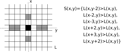
Figure 3: Mini-census Transform

When the right image $R(x,y)$ is used as the base, the matching cost is given as follows.

$$\begin{split}C^{R}(x,y,d)&=C^{R}_{AD}(x,y,d)+C^{R}_{MC}(x,y,d)\\ &=1-\exp(-\frac{|R(x,y)-L(x+d,y)|}{\lambda_{AD}})\hskip 5.0pt+\\ &\hskip 13.00005pt1-\exp(-\frac{MC(R(x,y),L(x+d,y))}{\lambda_{MC}})\\ &=C^{L}(x+d,y,d).\end{split}$$ (6)

This equation means that all $C^{R}(x,y,d)$ are already calculated when $C^{L}(x,y,d)$ are calculated, and $C^{L}(x,y,d)$ can be reused as $C^{R}(x-d,y,d)$.

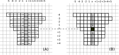
Figure 4: A cost aggregation method

III-C Cost Aggregation

The matching costs are aggregated as much as possible considering the similarity of the brightness of the pixels to compare the pixels as a block of the similar brightness. Fig.4 shows how the matching costs are aggregated. First, the matching costs are aggregated along the $x$-axis.

$$CA^{L}_{x}(x,y,d)=\sum^{+n}_{dx=-m}C^{L}(x+dx,y,d)$$ (7)

Here, m and n are the number of the continuous pixels with the similar brightness to $L(x,y)$ $(|L(x,y)-L(x+dx,y)|<\delta)$ on the left and right-side of $L(x,y)$. For example, in Fig.4, $m=3$ and $n=3$, because all pixels from $L(x-3,y)$ to $L(x+3,y)$ are similar to $L(x,y)$. Then, $CA^{L}_{x}(x,y,d)$ are aggregated along the $y$-axis as

$$CA^{L}(x,y,d)=\sum^{+N}_{dy=-M}CA^{L}_{x}(x,y+dy,d).$$ (8)

Here, $M$ and $N$ are the number of the continuous pixels with similar brightness to $L(x,y)$ on the upper and lower side of $L(x,y)$. In Fig.4, $M$ is 4 and $N$ is 4, because the pixels from $L(x,y-4)$ to $L(x,y+4)$ are similar to $L(x,y)$.

Then, $d$ which minimizes $CA^{L}(x,y,d)$ is chosen as the disparity at $L(x,y)$, and disparity map $D^{L}_{map}(x,y)$ is obtained.

$$D^{L}_{map}(x,y)=\min_{d}{CA^{L}(x,y,d)}.$$ (9)

By enlarging the range for summing up along the $x$- and $y$- axes, we can obtain more accurate disparities, though it requires more computation time.

III-D GCPs

In our approach, $D^{R}_{map}(x,y)$ is also calculated in the same way as $D^{L}_{map}(x,y)$. Then, ground control points, or GCPs, are obtained by comparing them [7]. Suppose that $D^{L}_{map}(x,y)=k$. This means that $L(x,y)$ and $R(x-k,y)$ showed the best matching when the left image is used as the base, and they are the same point of the object in the images. Therefore, $D^{R}_{map}(x-k,y)$ should also be $k$. If this requirement

$$D^{L}_{map}(x,y)=D^{R}_{map}(x-k,y)=k$$ (10)

is satisfied, the point is called a GCP, and it is considered that GCPs have higher reliability.

III-E Bilateral Estimation

Ideally, all pixels except for those in the occluded regions should be GCPs, however, in actuality more pixels become non-GCPs because of the slight change of the brightness between the input images. To achieve more reliable disparities of non-GCPs, two approaches are often used [10]. In both approaches, for each non-GCP, the closest GCPs on the left and right hand-side along the $x$-axis are searched first. Then, in the first approach, as shown in Fig.5(a), the closer GCP in the distance is chosen as the disparity of the non-GCP because the non-GCP and the closer GCP can be considered to belong to the same object with a higher probability. In the second approach, as shown in Fig.5(b), the smaller disparity is chosen as the disparity of the non-GCP assuming that the non-GCP is caused by the occlusion. The disparity of the occluded region is smaller than that of the foreground object because the disparity of the closer object is larger, and the non-GCP should have a smaller disparity. Both of these two methods can be easily implemented on GPU because of their high parallelism. However, due to their single function, the overall accuracy is not good enough.

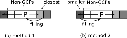
Figure 5: Non-GCPs Filling

In our system, we proposed a bilateral estimation methods to fill the non-GCPs as following steps:

1. Define the disparities of the GCP of $L(x-i,y)$ and $L(x+j,y)$ as $D(x-i,y)$ and $D(x+j,y)$.

2. If $|D(x-i,y)-D(x+j,y)|\leq{T}$, where $T$ is the threshold for the difference of disparity, it can be considered that the disparity is changing continuously in this range, and $D(x,y)$ is filled as:

   $$D(x-i,y)+i\cdot((D(x-i,y)-D(x+j,y))/(i+j)).$$ (11)

3. If $|D(x-i,y)-D(x+j,y)|>T$, which means that the disparity changes rapidly in this range, it can be considered that an edge exists in this range. Thus $D(x,y)$ is chosen as the $D(x-i,y)$ if $L(x-i,y)$ is closer to $L(x,y)$ than $L(x+j,y)$ in color, and otherwise, $D(x,y)$ is chosen as $D(x+j,y)$.

With this approach, we can fill the different areas in the different methods. Then, an accurate disparity map can be expected.

IV IMPLEMENTATION ON GPU

We have implemented the algorithm on Nvidia GTX780Ti. GTX780Ti has 15 streaming multi-processors (SMs). Each SM runs in parallel using 192 cores in it (2880 cores in total). GTX780Ti has two-layered memory system. Each SM has a 48KB shared memory, and one large global memory is shared among the SMs. The access delay to the shared memory is very short, but that to the global memory is very long. Therefore, the most important technique to achieve high performance on GPU is how to cache a part of the data on the shared memory, and to hide the memory access delay to the global memory. The shared and the global memory have the restriction of the access to them. In the CUDA, which is an abstracted architecture of Nvidia’s GPUs, 16 threads are managed as a set. When accessing to the global memory, 16 words can be accessed in parallel if the 16 threads access to continuous 16 words which start from 16 word-boundary. Otherwise, the bank conflict happens, and several accesses to the global memory happens. The shared memory consists of 16 banks, and in this case, the 16 words can be accessed in parallel if they are stored in the different memory banks (the addresses of the 16 words do not need to be continuous). For reducing the memory accesses to the global memory, the order of the calculation on GPU is different from the one described in the previous section.

• Step1 transfer the input images onto the GPU and scale down them

• Step2 compare the brightness of the pixels along the $x$-axis

• Step3 calculate the matching costs and aggregate them along the $x$-axis

• Step4 compare the brightness of the pixels along the $y$-axis

• Step5 aggregate the cost along the $y$-axis, and generate two disparity maps

• Step6 find GCPs by cross-checking

• Step7 apply median filter to remove noises and estimate the disparity map using bilateral method

• Step8 scale up the disparity map and transfer back to the CPU.

In the following discussion, $X_{org}\times{Y_{org}}$ is the image size ($X_{org}$ is the width, and $Y_{org}$ is the height), and $L_{org}[y][x]$ and $R_{org}[y][x]$ are the pixels in the left and right images. $L[y][x]$ and $R[y][x]$ are the pixels in the scaled-down images, and $X\times{Y}$ is the image size of them ($X=X_{org}/2$, $Y=Y_{org}/2$). Fig.6 shows the task assignment and input/output of each step. The details are discussed in the following subsections.

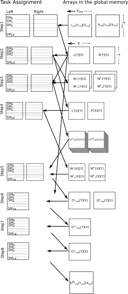
Figure 6: Task assignment of each step

IV-A Step1

The inputs to this step are $L_{org}[y][x]$ and $R_{org}[y][x]$, and they are transferred onto the global memory of the GPU, and are processed in parallel using 15 SMs.

1. $Y_{org}/15$ lines of both images are assigned to each SM as shown in Fig.7.

2. $X_{org}$ columns in the $Y_{org}/15$ lines are processed using $X^{\prime}$ ($X_{org}\leq{X^{\prime}}$) threads in the SM ($X^{\prime}$ must be a multiple of 64 because of the reason described below). When $X^{\prime}>X_{org}$, $X^{\prime}-X_{org}$ threads work in the same way as the $X_{org}$ threads, but generate no outputs.

3. When $X_{org}$ is larger than the maximum number of the threads in one SM (1024), each thread processes more than one columns. In our implementation, because the resolution of the input images are greater than 1024, each thread processes 2 columns during the scaling-down step.

For each pixel $L_{org}(x_{even},y_{even})$, both of the vertical and horizontal coordinates of which are even, all of the surrounding pixels $L_{org}(x_{even}+dx,y_{even}+dy)$ ($dx\in[-1,1]$, $dy\in[-1,1]$) are added together. Then, as the pixel value of the scaled-image, the average of the summation is stored in the global memory.

Figure 7: Mapping pixels to the threads

IV-B Step2

For $Y/15$ pixels in one column (let the pixels be $L[y_{b}+k][x_{b}]$($k=0,14$)), each thread compares its pixel’s value with its neighbors along the $x$-axis ($L[y_{b}+k][x_{b}+dx]$ ($dx=1,W_{x}$) and $L[y_{b}+k][x_{b}-dx]$ ($dx=1,W_{x}$)). The data type of $L[y][x]$ is $8b$ (unsigned char). Therefore, four continuous pixels are packed in one $32b$ word, and stored in the same memory bank of the shared memory. This means that these four continuous pixels can not be accessed in parallel owing to the memory access restriction of the shared memory. In order to avoid the bank conflict, Thread_i processes column ($i/(X/4)+(i\times{4})\%X$) as shown in Fig.7. In Fig.7, the first four pixels of each line ($L[y][0]$, $L[y][1]$, $L[y][2]$, $L[y][3]$) are stored in the first bank, and next four pixels ($L[y][4]$, $L[y][5]$, $L[y][6]$, $L[y][7]$) in the second bank. Thread₀ processes $Y/15$ pixels on $x=0$ ($L[y_{b}+dy][0]$ ($dy=0,14$)) sequentially, and Thread₁ processes $Y/15$ pixels on $x=4$ ($L[y_{b}+dy][4]$ ($dy=0,14$)) sequentially. By changing the order of the computation like this, bank conflict can be avoided. In our algorithm, all pixels can be processed independently, and the same results can be obtained regardless of the computation order.

In this method, four continuous pixels are stored in the same bank, and 16 threads are executed at the same time in CUDA. Therefore, $X$ must be a multiple of 64 ($4\times{16}$). When, $X$ is not the multiple of 64, larger $X$ which is the multiple of 64 is chosen, and the computation results for the extended part are discarded.

The outputs of this step are two integer values for each pixel, which show how many pixels are similar to the center pixel to the plus/minus direction of the $x$-axis. These values for $L[y][x]$ are stored in $W^{L}_{-}[y][x]$ and $W^{L}_{+}[y][x]$, and those for $R[y][x]$ are stored in $W^{R}_{-}[y][x]$ and $W^{R}_{+}[y][x]$. The data width of these arrays is $32b$, and the direct access to these values causes no bank conflict. $L[y][x]$ and $R[y][x]$ are transposed here, and stored in $L^{*}[x][y]$ and $R^{*}[x][y]$ respectively.

IV-C Step3

In this step, first, two matching costs ($C^{L}(x,y,d)$ and $C^{R}(x,y,d)$) are calculated, and then, they are aggregated along the $x$-axis using the range information in $W^{L}_{-}[y][x]$, $W^{L}_{+}L[y][x]$, $W^{R}_{-}[y][x]$ and $W^{R}_{+}[y][x]$ to calculate $CA^{L}_{x}(x,y,d)$ and $CA^{R}_{x}(x,y,d)$. Here, actually, we do not need to calculate $C^{R}(x,y,d)$ as described in Section 3.C because $C^{L}(x+d,y,d)$ can be used as $C^{R}(x,y,d)$. Therefore, all SMs are used to calculate $C^{L}(x,y,d)$ as shown in Fig.6-$step3$, and each SM processes $Y/15$ lines as follows.

1. For each of the Y/15 lines, repeat the following steps.

2. Set $d=0$.

3. Calculate $C^{L}(x,y,d)$ for all $x$ in the current line. $C^{L}(x,y,d)$ is stored in $C[x]$ (an array in the shared memory). For this calculation, 3 lines of $L[y][x]$ and $R[y][x]$ are cached in the shared memory for calculating the mini-census transform, and they are gradually replaced by the next line as the calculation progresses.

4. Calculate $CA^{L}_{x}(x,y,d)$ as follows.

   1. Set $CA_{x}[x]=C[x]$.

   2. Add $C[x+dx]$ to $CA_{x}[x]$ starting from $dx=1$ to the position given by $W^{L}_{+}[y][x]$.

   3. Add $C[x-dx]$ to $CA_{x}[x]$ starting from $dx=1$ to the position given by $W^{L}_{-}[y][x]$.

   4. Store $CA_{x}[x]$ into $CA^{*L}_{x}[d][x][y]$ in the global memory (note that this array is transposed).

5. Calculate $CA^{R}_{x}(x,y,d)$ as follows.

   1. Set $CA_{x}[x]=C[x+d]$.

   2. Add $C[x+d+dx]$ to $CA_{x}[x]$ starting from $dx=1$ to the position given by $W^{R}_{+}[y][x]$.

   3. Add $C[x+d-dx]$ to $CA_{x}[x]$ starting from $dx=1$ to the position given by $W^{R}_{-}[y][x]$.

   4. Store $CA_{x}[x]$ into $CA^{*R}_{x}[d][x][y]$ in the global memory (note that this array is transposed).

6. Increment $d$ if $d<D$, and go to step 3.

In this step, $D$ arrays are stored in the global memory.

IV-D Step4

$L[y][x]$ and $R[y][x]$ have been transposed and stored as $L^{*}[x][y]$ and $R^{*}[x][y]$ in step2. By using these arrays, the brightness of the pixels are compared efficiently along the $y$-axis. In this case, the pixel data (for example $L^{*}[x][y]$) are compared horizontally (parallel memory accesses are allowed only in this direction), and this means that $L^{*}[x][y]$ are compared with $L^{*}[x][y+dy]$ ($dy=-W_{y},W_{y}$). The range of the similar pixels are stored in $W^{*L}_{-}[x][y]$ and $W^{*L}_{+}[x][y]$ for $L^{*}[x][y]$, and in $W^{*R}_{-}[x][y]$ and $W^{*R}_{+}[x][y]$ for $R^{*}[x][y]$. $L^{*}[x][y]$ and $R^{*}[x][y]$ are processed in parallel as shown in Fig.6-$step4$, and each SM processes $X/15$ columns. The $Y$ lines in each column are assigned to $Y$ threads in the same way shown in Fig.7 though $x$ and $y$ are transposed.

IV-E Step5

In this step (Fig.6-$step5$), $CA^{*L}_{x}[d][x][y]$ and $CA^{*R}_{x}[d][x][y]$ are aggregated along the $y$-axis in parallel using $W^{*L}_{-}[x][y]$, $W^{*L}_{+}[x][y]$, $W^{*R}_{-}[x][y]$ and $W^{*R}_{+}[x][y]$, and then $D^{L}_{map}[y][x]$ and $D^{R}_{map}[y][x]$ (disparity maps when $L[y][x]$ and $R[y][x]$ are used as the base) are also generated as follows.

1. Each SM processes $X/15$ columns.

2. $Y$ threads in each SM processes $Y$ pixels in each of the $X/15$ columns.

3. Each thread repeats the following steps (in the following, only the steps for the left image are shown).

   1. Read $W^{*L}_{-}[x][y]$ and $W^{*L}_{+}[x][y]$ from the global memory.

   2. Set $d=0$.

   3. $Min[y]=$MAX_VALUE and $D_{map}[y]=0$.

   4. Calculate $CA^{L}(x,y,d)$ as follow.

      1. Set $CA[y]=CA^{*L}[d][x][y]$.

      2. Add $CA^{*L}_{x}[d][x][y+dy]$ to $CA[y]$ starting from $dy=1$ to the position given by $W^{*L}_{+}[x][y]$.

      3. Add $CA^{*L}_{x}[d][x][y-dy]$ to $CA[y]$ starting from $dy=1$ to the position given by $W^{*L}_{-}[x][y]$.

   5. If $CA[y]<Min[y]$ then $Min[y]=CA[y]$ and $D_{map}[y]=d$.

   6. Increment $d$ if $d<D$, and go to step 3(c).

   7. Store $D_{map}[y]$ in $D^{L}_{map}[y][x]$ in the global memory (note that his array is re-transposed).

IV-F Step6

In this step (Fig.6-$step6$), $D^{L}_{map}[y][x]$ and $D^{R}_{map}[y][x]$ are read from the global memory line by line, and the condition for the GCP (described in Section 3.D) is checked. In this step, each SM processes $Y/15$ lines. Thread_x first accesses $D^{L}_{map}[y][x]$, and then $D^{R}_{map}[y][+k]$ if $D^{L}_{map}[y][x]=k$. $k$ is different for each thread, and bank conflict happens in this step.

IV-G Step7

The median filter is applied using 15 SMs for the left image at first. Then, the bilateral estimation is used to fill the non-GCPs. If $D^{L}_{map}[y][x]$ is not a GCP, $thread_{x}$ scans $D^{L}_{map}[y][x]$ to the $+/-$ direction of the $x$-axis in order, and finds two GCPs (the GCPs closest on the left- and right-hand side). Then, the difference of the disparities of the two GCPs is calculated. If the difference is smaller than the threshold, the $D^{L}_{map}[y][x]$ is filled linearly according to the disparities of the two GCPs. If the different is larger than the threshold, the brightness of the two GCP are compared with the target pixel, and the disparity of the target pixel is replaced by the one which has similar brightness. Then, the improved disparity map $D^{+L}_{map}[y][x]$ is stored in the global memory.

IV-H Step8

Finally, the disparity map $D^{+L}_{map}[y][x]$ is scaled up by using the 15 SMs. In order to maintain a high accuracy, during the scaling-up along the $x$-axis, the bilateral estimation method described above is used again. On the other hand, the estimation along the $y$-axis is applied linearly. Then, the final disparity map $D^{fL_{org}}[y][x]$ is transferred back to the CPU.

TABLE I: Error rate when the cost aggregation range is changed (average error rate (%))

$W_{L}$$\backslash$$W_{R}$	$W_{y}=9$	$W_{y}=11$	$W_{y}=15$	$W_{y}=21$	$W_{y}=27$	$W_{y}=31$
$W_{x}=5$	25.10	24.98	24.83	24.68	24.62	24.61
$W_{x}=9$	24.67	24.55	24.4	24.3	24.26	24.26
$W_{x}=21$	24.39	24.34	24.21	24.13	24.1	24.09
$W_{x}=41$	24.53	24.38	24.29	24.21	24.19	24.17
$W_{x}=61$	24.53	24.5	24.41	24.32	24.31	24.28
$W_{x}=141$	24.6	24.55	24.48	24.42	24.38	24.28

TABLE II: Execution Time For The Middlebury Benchmark Set (ms)

Image	Size	Dmax	SD	$W^{LR}_{\pm}$	$W^{*LR}_{\pm}$	$C+CA_{x}$	CA	CC	Post	SU	Overall(GPU)	FPS
Adirondack(H)	$1436\times{992}$	145	0.035	0.149	0.317	10.443	13.943	0.437	0.181	0.09	25.595	40
Pipes(H)	$1482\times{994}$	128	0.038	0.135	0.289	19.8	11.44	0.506	0.238	0.09	32.536	31
Vintage(H)	$1444\times{960}$	380	0.038	0.143	0.315	26.142	36.394	0.092	0.221	0.087	63.432	16

Size: $W^{LR}_{\pm}=21$, $W^{*LR}_{\pm}=31$, $TC=13$ Dmax: Maximum Disparity SD: Scaling-Down. $W^{LR}_{\pm}$: Edge detection along the $x$-axis. $W^{*LR}_{\pm}$: Edge detection along the $y$-axis $C+CA_{x}$: cost calculation & Aggregation along the $x$-axis. CA: Aggregation along the $y$-axis. CC: Cross_check. Post: MedianFilter&Bilateral estimation. SU: Scaling-up. Overall: The overall time taken on GPU.

TABLE III: COMPARISON WITH HIGH-SPEED STEREO VISION SYSTEMS

System	Size	Dmax	Hardware	Benchmark	FPS	MDE/s
RT-FPGA[1]	$1920\times{1680}$	60	Kintex 7	Middlebury v2	30	5806
FUZZY[2]	$1280\times{1024}$	15	Cyclone II	Middlebury v2	76	1494
Low-Power[13]	$1024\times{768}$	64	Virtex-7	Middlebury v2	30	1510
ETE[3]	$1242\times{375}$	256	GTX TITAN X	KITTI 2015	29	3458
EmbeddedRT[8]	$640\times{480}$	128	Tegra X1	KITTI 2012	81	3185
MassP[4]	$1440\times{720}$	128	GPU	Middlebury v3	128	3981
Our system	$1436\times{992}$	145	GTX 780 Ti	Middlebury v3	40	7849

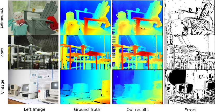
Figure 8: Processing results

V experimental results

We have implemented the algorithm on Nvidia GTX780Ti. The error rate and the processing speed are evaluated using Middlebury benchmark set [11].

In this evaluation, all parameters mentioned above affect the performance of the accuracy. According to our tuning results, we first set $\lambda_{AD}=0.3$, $\lambda_{MC}=2.3$ and $T=3$ to ensure a good accuracy. In the cost aggregation step, lower error rates can be expected by adding more cost along the $x$- and $y$- axes, though it requires more computation time, and makes the system slower. The maximum range of the cost aggregation $(W_{x},W_{y})$ can be changed when calculating $D^{L}_{map}$ and $D^{R}_{map}$. By changing them, the different criteria are used for the left and right image, and the GCPs can be more reliable. Table I shows the error rate (%) when the cost aggregation range is changed. In Table I, $W_{x}$ are the maximum aggregation range along the $x$-axis for the left and right images, and $W_{y}$ is the maximum aggregation range along the $y$-axis ($W_{y}$ is common to the left and right images). As shown in Table I, by enlarging $W_{y}$, the error rates can be improved when $W_{x}$ is small. We have fixed $W_{x}=21$ and $W_{y}=31$. To our best knowledge, the accuracy of our system is higher than other real-time systems (like [12]) which are listed in Middlebury Benchmark [11]. Additionally, we also compared our error rates with that obtained using the original size image set, which are processed using larger window ranges $W_{x}=41$ and $W_{y}=61$. According to our evaluation, the error rate (Bad 2.0) of our system (24.09%) is higher than that by the original size images (32.82%). One of the reasons is that we didn’t tuned the parameters $\lambda_{AD}$ and $\lambda_{MC}$ for the original image set. The other one is that in the scaling down images, some information that makes the matching difficult in the original size images, such as repetition of patterns and a serious of similar pixels, are discarded, and better matching becomes possible.

The processing speed of our system is almost proportional to the window size and the maximum disparity. Therefore, the computation time for ’Vintage’ becomes the slowest. Table II shows the processing speed of our system and its details. We ignore the time for CPU-GPU data transfers (less than 3% of the total elapsed time) since it can be overlapped with the computation. As shown in Table II, most of the computation time is used for the cost calculation and its aggregation ($C+CA_{x}$ and $CA$). $W^{LR}_{\pm}$, $W^{*LR}_{\pm}$, $CC$, $Post$, $SD$, $SU$ show the computation time for finding the cost aggregation range along the $x$- and $y$- axes, cross checking, post-processing and the image scaling. Unfortunately, for the ’Vintage’ set, its processing speed is 16fps due to the large disparity, and we cannot achieve the real-time processing.

Table III compares the processing speed of our system with other hardware systems. In Table III, all of the systems achieved a real-time processing as shown in FPS field, but their target image size (Size) and disparity range (Dmax) are different. According to the mega disparity evaluation per second (MDE/S), it can be noted that our system is much faster than other systems.

Fig.7 shows the results of our system for the two benchmark sets: Adirondack, Pipes and Vintage.

VI Conclusion

In this paper, we have proposed a real-time stereo vision system for high resolution images on GPU. Its processing speed is much faster than previous one. At the same time, it also maintained a high accuracy. In our current implementation, the processing speed is still limited by the access delay to the global memory. To improve the processing speed so that the real-time processing can be achieved slower GPUs is our main future work.

References

- [1] Daolu Zha, Xi Jin, Tian Xiang: A real-time global stereo-matching on FPGA. Microprocessors and Microsystems - Embedded Hardware Design 47: 419-428 (2016)
- [2] Madaín Pérez Patricio and Abiel Aguilar-González and Miguel O. Arias-Estrada and Héctor-Ricardo Hernandez-de Leon and Jorge-Luis Camas-Anzueto and J. A. de Jesús Osuna-Coutiño: An FPGA stereo matching unit based on fuzzy logic. Microprocessors and Microsystems - Embedded Hardware Design 42: 87-99 (2016)
- [3] Alex Kendall, Hayk Martirosyan, Saumitro Dasgupta, Peter Henry, Ryan Kennedy, Abraham Bachrach, Adam Bry: End-to-End Learning of Geometry and Context for Deep Stereo Regression. CoRR abs/1703.04309 (2017)
- [4] Wenbao Qiao and Jean-Charles Créput: Stereo Matching by Using Self-distributed Segmentation and Massively Parallel GPU Computing. ICAISC (2) 2016: 723-733
- [5] Jure Zbontar, Yann LeCun: Stereo Matching by Training a Convolutional Neural Network to Compare Image Patches. Journal of Machine Learning Research 17: 65:1-65:32 (2016)
- [6] Xiaoqing Ye, Jiamao Li, Han Wang, Hexiao Huang, Xiaolin Zhang: Efficient Stereo Matching Leveraging Deep Local and Context Information. IEEE Access 5: 18745-18755 (2017)
- [7] Aaron F. Bobick, Stephen S: Intille: Large Occlusion Stereo. International Journal of Computer Vision 33(3): 181-200 (1999)
- [8] Daniel Hernández Juárez and Alejandro Chacón and Antonio Espinosa and David Vázquez and Juan Carlos Moure and Antonio M. López: Embedded Real-time Stereo Estimation via Semi-Global Matching on the GPU. ICCS 2016: 143-153
- [9] Minxi Jin, Tsutomu Maruyama: Fast and Accurate Stereo Vision System on FPGA. TRETS 7(1): 3:1-3:24 (2014)
- [10] Qingxiong Yang and Liang Wang and Ruigang Yang and Henrik Stewénius and David Nistér: Stereo Matching with Color-Weighted Correlation, Hierarchical Belief Propagation, and Occlusion Handling. IEEE Trans. Pattern Anal. Mach. Intell. 31(3): 492-504 (2009)
- [11] D.Scharstein and R.Szeliski: http://vision.middlebury.edu/stereo/eval3/.
- [12] Leonid Keselman, John Iselin Woodfill, Anders Grunnet-Jepsen, Achintya Bhowmik: Intel RealSense Stereoscopic Depth Cameras. CoRR abs/1705.05548 (2017)
- [13] Luca Puglia, Mario Vigliar, Giancarlo Raiconi: Real-Time Low-Power FPGA Architecture for Stereo Vision. IEEE Trans. on Circuits and Systems 64-II(11): 1307-1311 (2017)
- [14] Lu Zhang, Ke Zhang, Tian Sheuan Chang, Gauthier Lafruit, Georgi Krasimirov Kuzmanov, Diederik Verkest: Real-time high-definition stereo matching on FPGA. FPGA 2011: 55-64
- [15] Ke Zhang, Jiangbo Lu, Gauthier Lafruit: Cross-Based Local Stereo Matching Using Orthogonal Integral Images. IEEE Trans. Circuits Syst. Video Techn. 19(7): 1073-1079 (2009)
- [16] Edoardo Paone, Gianluca Palermo, Vittorio Zaccaria, Cristina Silvano, Diego Melpignano, Germain Haugou, Thierry Lepley: An exploration methodology for a customizable OpenCL stereo-matching application targeted to an industrial multi-cluster architecture. CODES+ISSS 2012: 503-512