Efficient Stereo Matching on Embedded GPUs with Zero-Means Cross Correlation

Abstract

Mobile stereo-matching systems have become an important part of many applications, such as automated-driving vehicles and autonomous robots. Accurate stereo-matching methods usually lead to high computational complexity; however, mobile platforms have only limited hardware resources to keep their power consumption low; this makes it difficult to maintain both an acceptable processing speed and accuracy on mobile platforms. To resolve this trade-off, we herein propose a novel acceleration approach for the well-known zero-means normalized cross correlation (ZNCC) matching cost calculation algorithm on a Jetson Tx2 embedded GPU. In our method for accelerating ZNCC, target images are scanned in a zigzag fashion to efficiently reuse one pixel’s computation for its neighboring pixels; this reduces the amount of data transmission and increases the utilization of on-chip registers, thus increasing the processing speed. As a result, our method is 2X faster than the traditional image scanning method, and 26% faster than the latest NCC method. By combining this technique with the domain transformation (DT) algorithm, our system show real-time processing speed of 32 fps, on a Jetson Tx2 GPU for 1,280x384 pixel images with a maximum disparity of 128. Additionally, the evaluation results on the KITTI 2015 benchmark show that our combined system is more accurate than the same algorithm combined with census by 7.26%, while maintaining almost the same processing speed.

I INTRODUCTION

Stereo matching is a key algorithm for depth detection in computer vision, but its usability is still limited because attaining high accuracy requires a very high computational complexity. By achieving both high accuracy and processing speed on mobile platforms, it can be used in many applications, including auto-driving, autonomous robots, and so on.

Thus far, many researchers have focused upon accelerating stereo matching on mobile platforms. Most of them focus on accelerating the two most computationally intensive stages: cost calculation and cost aggregation. During cost calculation, each pixel in the reference image is first matched with several pixels in the target image one by one. Next, the similarity between any two pixels is quantified by a numerical value (cost) calculated by a matching method, such as the sum of absolute differences (SAD), census, or convolution neural network (CNN). Then, to further improve the accuracy of the matching system, the cost of each pixel within a certain region is expected to be aggregated together to represent the similarity between any two regions; this is called matching-cost aggregation. Many methods can be used to determine the range of the matching regions, such as semi-global matching (SGM) or domain transformation (DT). Various combinations of the above two stages not only result in different matching accuracies, but also different computational complexities; this leads to differing processing speeds.

Many researches implement their stereo-matching systems on FPGAs, respectively. Wang [1] first combines a simplified SGM with the simple absolute differences and census matching algorithms, processing 1,024x768 pixel images with 96 disparities at 67 fps. Mohammad [2], Zhang [3] and Kuo [4] use the census algorithm to calculate their matching costs. Mohammad [2] combines census with a cross-aggregation method to achieve a good error rate of less than 9.22% and a high processing speed of faster than 200 fps on the KITTI 2015 benchmark [5]. Zhang [3] uses a box filter to aggregate matching costs and achieves a high processing speed of 60 fps for 1080p images. Kuo [4] uses a two-pass aggregation method and achieves the same processing speed as  [3]. Oscar [6] uses SAD to calculate the matching cost and combines it with SGM. Due to SGM’s high accuracy for even the simple SAD matching algorithm, it can still achieve a lower error rate of 8.7%, except that its speed is reduced to 50 fps. Additionally, Zhang [7] develops a special ASIC to accelerate the implementation of SGM and achieves a processing speed of 30fps for 1080p images. Here, due to the limitations of floating-point decimal calculation, both the FPGA-based and the dedicated ASIC-based systems usually use methods such as SAD and census to obtain integer cost values. Although this is conducive to implementation on them, it also limits improvement in the matching accuracy. Furthermore, hardware-based systems typically need long development cycles and are also difficult to maintain. The recent advent of embedded GPUs has allowed the development of many systems [8] [9]. Compared to FPGAs, embedded GPU-based systems have short development cycles [10]. In addition, they are easy to maintain and port on other platforms. Wang [11], Smolyanskiy [12] and Tonioni [13] implement their systems on a Jetson Tx2 embedded GPU using the CNN; according to the evaluation results of KITTI 2015 [5] benchmark, their accuracies are high, with error rates between 3.2% and 6.2%. However, due to the significant calculations of CNN-based methods, their processing speeds are only a few fps, far below the requirements for practical applications. Daniel [14] constructs a fast stereo-matching system on a Jetson Tx2 GPU. It also combines census algorithm with SGM to achieve an error rate of 8.66% and a processing speed of 29 fps on KITTI 2015 benchmark. It is currently the best system for balancing the accuracy and processing speed on mobile GPUs; however, due to the census-matching method, this system is still not accurate enough, even if implemented on GPUs that are good at floating-point decimal calculations.

According to [15], the matching accuracy by normalized cross correlation (NCC) is better than that by census because it has a higher ability to withstand changes in gain and bias. Furthermore, zero-means NCC (ZNCC)–an improved version of NCC–provides strong robustness because it also tolerates uniform brightness variations [16][17]. However, ZNCC has not been widely used on the mobile systems with limited hardware resources because of its higher computational complexity.

In this paper, we accelerate ZNCC on a Jetson Tx2 embedded GPU and make it possible to achieve a comparable processing speed to that of census with a higher matching accuracy. The main contributions of this paper are as follows:

• We introduce a new calculation method, zigzag scanning based zero-means normalized cross correlation (Z²-ZNCC) to reuse the computational results of a pixel for the calculations of its neighbors. This makes it possible to reduce data transfer between the global memory of the GPU and increase the processing speed.

• We propose a strategy to make efficient use of registers during zigzag scanning to achieve higher parallelism of GPU threads driven by GPU cores.

• We design GPU-implementation algorithms for two parallel summation methods used in our Z²-ZNCC and comprehensively compare their performance.

• We create FastDT, an upgraded version of the GPU-based domain transformation method presented in [18] by removing the cost-value shifting step and increasing the flag code. Then, we combine it with Z²-ZNCC to construct a real-time stereo-matching system on an embedded GPU.

The experimental results demonstrate that our method is 2X faster than the traditional image-scanning method and 26% faster than the latest NCC method [19]. Furthermore, our system achieves a processing speed of 32 fps and an error rate of 9.26% for 1,242x375 pixel images when the maximum disparity is 128 on a KITTI 2015 dataset. It is one of the few embedded GPU-based real-time systems, with an accuracy much higher than others.

This paper extends our previous work (short paper) [20] from the following aspects.

• We design two parallel summation methods which maximize the processing speed of Z²-ZNCC depending on the template size.

• We introduce an efficient two-step implementation technique for domain transformation, which not only maintains a high processing speed, but also a high accuracy of Z²-ZNCC.

• We conduct comprehensive experiments to examine the impact of various conditions on the processing speed of Z²-ZNCC.

The rest of the paper is organized as follows. Section II introduces the related works. Section III reviews ZNCC and DT calculation methods. Section IV discusses the GPU implementation of Z²-ZNCC and FastDT. Section V shows the evaluation results. Finally, Section VI presents the conclusions and our future work.

II Related works

Recently, many researchers have focused upon accelerating the performance of NCC-based methods and applying them into stereo-matching systems.

Lin [21] proposes an optimization method for ZNCC calculation on a general platform. This method divides the standard equation into four independent parts and calculates the correlation coefficient efficiently using sliding windows. Hence, the computational complexity of ZNCC could be reduced from the original order. The computation time becomes constant for the window size; however, a large memory is required to store the calculation results for reuse. Although this method works nearly 10X faster than traditional ones, it is not applicable to embedded GPUs because of their limited memory space.

Rui [22] implements a fast ZNCC-based stereo-matching system on GTX 970M GPU. This work focuses on the use of integral images to calculate the mean and standard deviation efficiently. Rui’s system runs approximately 9X faster than a single-threading CPU implementation and about 2X faster than eight-threading; however, according to our evaluation, this approach is inefficient for a small-size window (less than 9x9) because obtaining an integral image itself also requires calculation costs. These costs are mainly caused by data transfer of the integration results, which cannot be ignored for an embedded GPU with a high memory latency.

Han [19] implements an NCC-based stereo-matching system on a Jetson Tx2 GPU. This method divides the equation into three parts, each with an identical control flow but different data locations. All intermediate results are stored on shared memory evenly so as to accelerate the calculation through reuse. However, as mentioned in Section I, the heavy use of shared memory reduces the parallelism of GPU blocks.

III Algorithms and Optimizations

III-A Zero-means Normalized Cross Correlation (ZNCC)

ZNCC is used to calculate matching costs between a reference pixel $I_{R}(x,y)$ in the reference image and a series of target pixels $I_{T}(x-d,y)$ in the target image. $d$ is called disparity, and its range is $[0,D)$, where $D$ is a constant called maximum disparity. The function of ZNCC is given as follows:

$$C(x,y,d)=\frac{\displaystyle\sum_{(x,y)\in{W}}{\Delta{I_{R}}(x,y)\cdot{\Delta{I_{T}}(x-d,y)}}}{\sigma_{R}(x,y)\cdot{\sigma_{T}(x-d,y)}},$$ (1)

where

$$\begin{split}\sigma_{R}(x,y)&=\sqrt{\displaystyle\sum_{(x,y)\in{W}}{\Delta{I_{R}(x,y)^{2}}}},\\ \sigma_{T}(x-d,y)&=\sqrt{\displaystyle\sum_{(x,y)\in{W}}{\Delta{I_{T}(x-d,y)^{2}}}},\\ \end{split}$$

and

$$\begin{split}\Delta{I_{R}(x,y)}&=I_{R}(x,y)-\overline{I_{R}(x,y)},\\ \Delta{I_{T}(x-d,y)}&=I_{T}(x-d,y)-\overline{I_{T}(x-d,y)}.\\ \end{split}$$

Here, $\overline{I_{R}(x,y)}$ and $\overline{I_{T}(x-d,y)}$ are the averages of the pixel values in the matching windows $W$ surrounding $I_{R}(x,y)$ and $I_{T}(x-d,y)$, respectively. $C(x,y,d)$ in (1) is the correlation coefficient (i.e., the matching cost) between $I_{R}(x,y)$ and $I_{T}(x-d,y)$; its range is $[0,1]$ (the closer to one, the more similar the two windows). $\sigma_{R}(x,y)$ and $\sigma_{T}(x-d,y)$ are the standard deviations of the pixel values in the two windows and are used to normalize the correlation coefficient between them. Each reference pixel $I_{R}(x,y)$ needs to be matched with $D$ target pixels $I_{T}(x-d,y)$; here, $\Delta{I_{R}(x,y)}$ and $\Delta{I_{T}(x-d,y)}$ can be calculated in advance because the calculations of these terms are closed in each image. As such, the total number of calculations can be reduced. However, when the size of the matching window $W$ is $l^{2}$ (where $l=2r+1$ represents the side length of window $W$) $l^{2}$-times the memory space is needed for each image because each window has $l^{2}$ differences.

To further reduce the ZNCC’s computation complexity, (1) can be rewritten as follows:

$$\begin{split}C(x,y,d)=\frac{\displaystyle\sum_{(x,y)\in{W}}{\Pi_{RT}(x,y,d)}-l^{2}\cdot{\overline{\Pi_{RT}(x,y,d)}}}{\sigma_{R}(x,y)\cdot{\sigma_{T}(x-d,y)}},\end{split}$$ (2)

where

$$\begin{split}\Pi_{RT}(x,y,d)&=I_{R}(x,y)\cdot{I_{T}(x-d,y)},\\ \overline{\Pi_{RT}(x,y,d)}&=\overline{I_{R}(x,y)}\cdot{\overline{I_{T}(x-d,y)}},\\ \end{split}$$

and

$$\begin{split}\sigma_{R}(x,y)&=\sqrt{\displaystyle\sum_{(x,y)\in{W}}{I_{R}(x,y)^{2}}-l^{2}\cdot{\overline{I_{R}(x,y)}^{2}}},\\ \sigma_{T}(x-d,y)&=\sqrt{\displaystyle\sum_{(x,y)\in{W}}{I_{T}(x-d,y)^{2}}-l^{2}\cdot{\overline{I_{T}(x-d,y)}^{2}}}.\\ \end{split}$$

In this calculation, $C(x,y,d)$, $\sigma_{R}(x,y)$, and $\sigma_{T}(x-d,y)$ are calculated from four values; $\overline{I_{R}(x,y)}^{2}$, $\sum{I_{R}(x,y)^{2}}$, $\overline{I_{T}(x-d,y)}^{2}$, and $\sum{I_{T}(x-d,y)^{2}}$, rather than from $\Delta{I_{R}(x,y)}$, and $\Delta{I_{T}(x-d,y)}$ as shown in (1). These four values are only related to their respective images and can all be calculated in advance. Thus, both $\sigma_{R}(x,y)$ and $\sigma_{T}(x-d,y)$ can be calculated efficiently without calculating $\Delta{I_{R}(x,y)}$ and $\Delta{I_{T}(x-d,y)}$ for each pixel $l^{2}$ times. This transformation not only helps to reduce the total calculation amount, but also reduce the required memory space.

Of course, ZNCC-based matching is performed in a fixed size window, which is not accurate for irregular patterns in reality; therefore, the matching cost $C(x,y,d)$ is usually combined with various aggregation methods to improve the matching accuracy.

III-B Domain Transformation (DT)

In cost aggregation step, the matching costs of all similar pixels in the same area (e.g., the area within the pink-dashed line in Fig.1 (a)) are added together. Domain Transformation (DT) [23] is an effective algorithms for use at this stage. Unlike other algorithms, DT avoids over-fitting of cost propagation by using the gradients of adjacent pixels to weight their costs in different directions, rather than judging the boundary of each area in advance. The advantage of DT is that there is no need to segment each area for cost aggregation separately, and it is suitable for parallel processing to increase the aggregation speed. In DT, the matching cost of each pixel is aggregated from four different directions, while propagating its cost to four neighboring pixels is done according to the following equations:

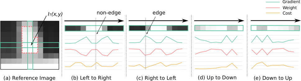
Figure 1: Domain transformation

$$C_{L}(x,y,d) =C(x,y,d)\small{+}C_{L}(x\small{-}1,y,d)\cdot{W_{L}(x,y)},$$ (3)

$$C_{R}(x,y,d) =C_{L}(x,y,d)\small{+}C_{R}(x\small{+}1,y,d)\cdot{W_{R}(x,y)},$$ (4)

$$C_{U}(x,y,d) =C_{R}(x,y,d)\small{+}C_{U}(x,y\small{-}1,d)\cdot{W_{U}(x,y)},$$ (5)

$$C_{D}(x,y,d) =C_{U}(x,y,d)\small{+}C_{D}(x,y\small{+}1,d)\cdot{W_{D}(x,y)}.$$ (6)

Here, $C_{L}$, $C_{R}$, $C_{U}$, and $C_{D}$ represent the aggregated costs for each pixel from four different directions (left, right, up, and down). In this aggregation, for example, the boundary condition for (3) is given by $C_{L}(0,y,d)=C(0,y,d)$. $W_{L}$, $W_{R}$, $W_{U}$ and $W_{D}$ represent the corresponding weights calculated by the gradient between adjacent pixel values according to the following equations:

$$W_{L}(x,y)=a^{1+\frac{\sigma_{s}}{\sigma_{r}}\cdot{|I_{T}(x,y)-I_{T}(x-1,y)|}},$$ (7)

$$W_{R}(x,y)=a^{1+\frac{\sigma_{s}}{\sigma_{r}}\cdot{|I_{T}(x,y)-I_{T}(x+1,y)|}},$$ (8)

$$W_{U}(x,y)=a^{1+\frac{\sigma_{s}}{\sigma_{r}}\cdot{|I_{T}(x,y)-I_{T}(x,y-1)|}},$$ (9)

and

$$W_{D}(x,y)=a^{1+\frac{\sigma_{s}}{\sigma_{r}}\cdot{|I_{T}(x,y)-I_{T}(x,y+1)|}},$$ (10)

where

$$a=\exp{(-\frac{1}{\sigma_{s}})}.$$ (11)

In (7) to (11), $\sigma_{s}$ is a spatial parameter and $\sigma_{r}$ is an intensity range parameter. Both are used to adjust the weight caused by gradient changes in space and intensity.

To simplify the calculation, the weight equations can be further simplified below (here, we only take (7) as an example):

$$\ln{W_{L}} =\ln{(a^{1+\frac{\sigma_{s}}{\sigma_{r}}\cdot{|I_{T}(x,y)-I_{T}(x-1,y)|}})}$$

$$=(1+\frac{\sigma_{s}}{\sigma_{r}}\cdot{|I_{T}(x,y)-I_{T}(x-1,y)|})\cdot{\ln{a}}$$

$$=(1+\frac{\sigma_{s}}{\sigma_{r}}\cdot{|I_{T}(x,y)-I_{T}(x-1,y)|})\cdot{(-\frac{1}{\sigma_{s}})}$$

$$=-\frac{1}{\sigma_{s}}-\frac{|I_{T}(x,y)-I_{T}(x-1,y)|}{\sigma_{r}},$$

then

$$W_{L} =\exp(-\frac{1}{\sigma_{s}}-\frac{|I_{T}(x,y)-I_{T}(x-1,y)|}{\sigma_{r}})$$

$$=K\cdot{\exp(-\frac{|I_{T}(x,y)-I_{T}(x-1,y)|}{\sigma_{r}})},$$

where

$$K=\exp(-\frac{1}{\sigma_{s}}).$$ (14)

$K$ is a constant coefficient used to ease the calculation of $W_{L}$.

Figure.1 shows an example of cost aggregation for pixel $I_{T}(x,y)$. Figure.1 (a) shows part of the reference image centered on $I_{T}(x,y)$. Figures.1 (b) to 1 (e) show the cost propagation process from different directions. Three curves with different colors represent the changes in the gradient, weights, and propagated costs, respectively. According to (III-B), the weight is calculated by the gradient and then used to weight the propagated cost value. As shown in Figs.1 (b) to 1 (e), the weight changes in the opposite direction to the change in gradient value, thereby ensuring that cost propagation can be performed normally among non-edge pixels (Fig.1 (b)) and can also be interrupted at edge pixels (Fig.1 (c)). When the propagation from down to up is completed (i.e., when the final aggregation result $C_{D}(x,y,d)$ is obtained), $C(x,y,d)$ is replaced by $C_{D}(x,y,d)$, and used in the following stages.

III-C Winner-Take-ALL (WTA)

After calculating matching cost for maximum disparity $D$ times, the target pixel $I_{T}(x-d,y)$ that is most similar to reference pixel $I_{R}(x,y)$ is determined as:

$$D_{map}(x,y)=\mathop{\rm arg~{}min}\limits_{d}{(1-C(x,y,d))}.$$ (15)

As shown in this equation, the value of $d$ that minimizes $(1-C(x,y,d))$ is chosen as the disparity of the reference pixel $I_{R}(x,y)$.

IV Implementation

Implementing ZNCC and DT on an embedded GPU is a key challenge for realizing a fast and accurate mobile stereo-vision system. In this section, we first introduce the architecture of Jetson Tx2 GPU; then, we describe the acceleration approaches of ZNCC and DT, respectively.

IV-A GPU Architecture and CUDA Programming Model

The Jetson Tx2 has 2 streaming multi-processors (SMs); each SM runs in parallel using 128 cores (256 cores in total) and has two types of on-chip memory: register memory and shared memory. Their sizes are limited, but their access latencies are very low. This GPU also has a global memory (off-chip), which is usually used to hold all data for processing. Due to the high latency of access to the off-chip memory, the most important point for achieving high performance on the GPU is to minimize the amount of data transfer between on-chip and off-chip memory.

In our implementation, we use the GPGPU programming model CUDA [24]. CUDA abstractly defines the GPU core, SM, and GPU itself as thread, block, and grid, respectively. A grid is composed of blocks and a block is composed of threads. Every 32 threads execute the same instruction, which is called a warp. The warps are scheduled serially by the SMs. Users can define the number of the abstract resources according to their requirements, which may exceed the physical GPU resources; then, the CUDA driver schedules abstract resources to work upon physical resources. Since the total number of registers and shared-memory space are fixed, the amount of these resources allocated to each thread and block determines how many of them can be active. The more allocated, the fewer threads and blocks can be activated, which resulting in reduced performance. By storing intermediate calculation results and reusing them afterwards, the total amount of calculation can be reduced; however, more hardware resources are needed to store these results, which limits the number of active threads. On the other hand, by recalculating them each time, the required amount of hardware resources can be reduced, and more threads can be active. Balancing the hardware-resource usage and total amount of calculation is a key point for achieving high performance, especially on embedded GPUs with limited hardware resources.

IV-B Implementation of ZNCC

Our ZNCC-acceleration approach includes two steps: (1) calculation of the means and the sums of squares in matching windows, and (2) calculation of the correlation coefficients of each pixel by zigzag scanning.

IV-B1 Summation

For the ZNCC-acceleration approach, the means and sums of squares in each matching window are calculated in advance (Section III-A). Taking the example of the pixel values in the reference image, we describe the two methods as follows (for simplicity, we only describe the sum in the reference image):

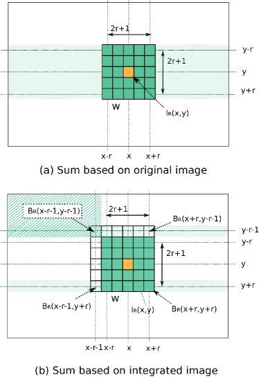
Figure 2: Summation methods

Method 1: As shown in Fig.2 (a), $S_{R}(x,y)$, the sum of the pixel values in each matching window $W$ is calculated as follows:

$$\begin{split}S_{R}(x,y)&=\displaystyle\sum_{(x,y)\in W}I_{R}(x,y).\\ \end{split}$$ (16)

Here, $(2r+1)^{2}$ pixel values are simply added around the center pixel $I_{R}(x,y)$.

The summation of each window is performed independently by different CUDA threads. Since the two adjacent windows for two adjacent pixels share $2r\times{(2r+1)}$ pixels, the data from $(2r+1)$ rows or columns are excepted to be cached in the same shared memory. The allocated memory space grows as the window size increases. The number of columns and rows processed by each CUDA block at the same time depends upon the size of the shared memory allocated; for smaller-sized windows, less hardware resources are required for each thread, and higher parallelism can be expected; however, as the window size increases, more hardware resources are required, and fewer threads can be active. Therefore, this method is not suitable for the summation of large windows.

Method 2: This method performs the summation using the integral image $B_{R}(x,y)$:

$$B_{R}(x,y)=\sum_{u=0}^{x}\sum_{v=0}^{y}I_{R}(u,v).$$ (17)

As shown in Fig.2 (b), $S_{R}(x,y)$ is calculated using four points in the integral image, regardless of the window size:

$$\begin{split}S_{R}(x,y)&{\small=}B_{R}(x+r,y+r)+B_{R}(x{\small-}r{\small-}1,y{\small-}r{\small-}1)\\ &{\small-}B_{R}(x+r,y{\small-}r{\small-}1){\small-}B_{R}(x{\small-}r{\small-}1,y+r).\end{split}$$ (18)

In this calculation method, To calculate the sum for the pixels on row $y$, only two rows ($y-r-1$ and $y+r$) of the integral image are needed. Thus, this method is suitable for the summation of large windows.

Obtaining an integral image in parallel requires two steps:

1. integrate each row of $I_{R}$, defined as $B_{H}$,

2. integrate each column of $B_{H}$, defined as $B_{R}$.

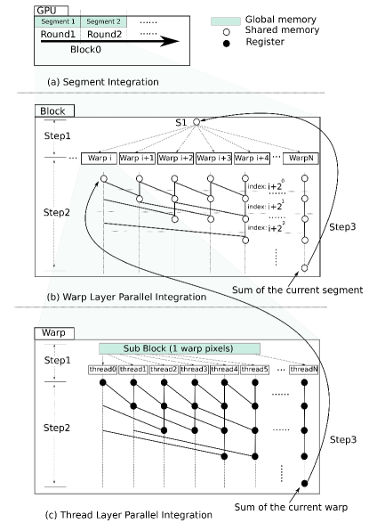
Figure 3: Integration along the $x$-axis

To generate the integral image, all image data need to be loaded from global memory to the shared memory. However, due to the limitation of the shared memory, the pixels in one row are divided into several segments and integrated partly as shown in Fig.3 (a). Considering the limitations of data sharing between different GPU blocks, we only use one block (Block0 in Fig.3 (a)) for the integration of one row, which means that each segment is integrated by the same block one by one (Round1, Round2,…) rather than processing multiple blocks in parallel. In each block, a two-layer parallel-integration strategy based on the Kogge-Stone Adder algorithm is used as shown in Fig.3 (b) and (c), since the threads work in the units of warp. The Kogge-Stone Adder method is used because of its high computational efficiency and suitability for thread-level parallel operations on GPUs. It is not necessary to check the parity of the operand index for each stage.

Figure.3 (b) shows the parallel integration on the Warp layer. In Fig.3 (b), “$\circ$” denotes the shared memory used in the current segment. Before integration, all threads in each warp are initialized with a variable $S1$, which represents the sum of the previous segment (step 1). For the first segment in one row, $S1$ is initialized to 0. Then, each warp performs the integration independently and propagates its intermediate results by shared memory according to the Kogge-Stone Adder method (step 2). In this step, the result of each Warp $i$ is added to Warp $i+2^{t-1}\ (i+2^{t-1}<N)$ through the shared memory, with $t$ representing the number of repetitions increasing from 1 to $\lfloor{\log_{2}{N}\rfloor}$ and $N$ representing the number of threads in each warp. Then, the sum of the current segment is updated by the last thread (step 3); at the same time, the integrated result of each thread is transferred to the global memory for the integration along the $y$-axis.

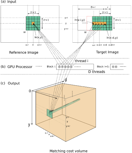
Figure 4: Stereo matching on the GPU

Figure.3 (c) shows the parallel integration on the Thread layer. After the initialization shown in Fig.3 (b) step1, each thread loads the corresponding pixel value from the global memory to the registers represented by “$\bullet$”, and adds it to the initial value $S1$. Then, integration is performed through the register shift among the threads in the same warp using the method shown in Fig.3 (b) step 2, and the last result is stored in the shared memory.

By repeating the above steps until the integration of the last segment ends, the integral image of each row can be calculated and used to obtain the entire integral image along the $y$-axis. Here, by transposing the matrix [25], integration can be transformed from vertical to horizontal. However, this may be less effective than a direct calculation when the vertical range is small, because the memory overhead required by matrix transposition itself reduces the parallelism of the GPU blocks. In this paper, we perform a sequential column-wise integration rather than using a parallel-computing method, because the height of the image set is less than 400 pixels.

IV-B2 Z²-ZNCC on Stereo Matching

After the summations above, the terms in (2) can be easily calculated with the exception of $\sum_{(x,y)\in W}{\Pi_{RT}(x,y,d)}$ is omitted in the following discussion to simplify the description. Here, we show that $\sum{\Pi_{RT}(x,y,d)}$ can be calculated efficiently by scanning the image in a zigzag fashion. Unlike the other summations, $\Pi_{RT}(x,y,d)$ represents a 3D-matching result between reference pixels and multiple target pixels under different disparities. Efficient calculation of $\sum{\Pi_{RT}(x,y,d)}$ is the most critical part of our implementation.

Task Assignment

As shown in Fig.4 (a), $I_{R}(x,y)$ is matched with $D$ pixels $I_{T}(x-d,y)$. To calculate $\sum{\Pi_{RT}(x,y,d)}$ for each $I_{R}(x,y)$, $(2r+1)^{2}$ pixels around $I_{R}(x,y)$ and $(2r+1)\times{(D+2r)}$ pixels around $I_{T}(x-d,y)\ (d\in[0,D))$ are required. For this matching, one block is assigned because the pixel data loaded into the shared memory can be reused to match adjacent pixels. In each block, $D$ threads are assigned to perform the matching in parallel for each corresponding $d$, as shown in Fig.4 (b). Each thread $i$ calculates $\sum{\Pi_{RT}(x,y,i)}$ using the pixels in the windows $W$ (centered at $I_{R}(x,y)$) and windows $W^{\prime}$ (centered at $I_{T}(x-i,y)$). Here, $\Pi_{RT}(x,y,i)$ is calculated element by element, and their sum is calculated efficiently via our approach described below. After calculating $\sum{\Pi_{RT}(x,y,d)}$ (as shown in Fig.4 (c)), the matching cost $C(x,y,d)$ can be calculated according to (2) and then stored in the global memory for use in the cost-aggregation stage. With this task assignment, the data once loaded to the shared memory from the global memory can be efficiently reused for the calculation of adjacent pixels when $D$ is sufficiently large.

Zigzag Scanning

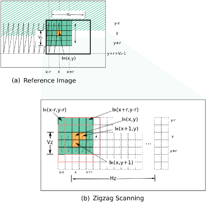
Figure 5: Zigzag scanning

In our approach, the image is scanned in a zigzag fashion, as shown in Fig.5 (a) along the $x$ and $y$ axis, while $\sum{\Pi_{RT}(x,y,d)}$ is calculated for each pixel in parallel along the $d$-axis. $V_{Z}$ pixels in a column are processed first from top to bottom; then, the same processing is repeated on the next column. This scanning method is repeated from left to right. In this zigzag scanning, the rows are segmented in the same way as in summation Method 2, and $(2r+V_{Z})\times{(2r+H_{Z})}$ pixels in the reference image and $(2r+V_{Z})\times{(2r+H_{Z}+D)}$ pixels in the target image are loaded into the shared memory respectively as shown in Fig.5 (b) (where $H_{z}$ is a constant decided by the shared-memory size). With this zigzag scanning, after $\sum{\Pi_{RT}(x,y,d)}$ was calculated, $\sum{\Pi_{RT}(x,y+1,d)}$ and $\sum{\Pi_{RT}(x+1,y,d)}$ can be easily calculated as follows:

$$\begin{split}\sum_{(x,y)\in W}{\Pi_{RT}(x,y{\small+}1,d)}&{\small=}\displaystyle\sum_{\Delta{x}{\mbox{\scriptsize=}}-r}^{r}{\sum_{\Delta{y}{\mbox{\scriptsize=}}-r}^{r}{\Pi_{RT}(x{\small+}\Delta{x},y{\small+}\Delta{y},d)}}\\ &{\small+}\displaystyle\sum_{\Delta{x}=-r}^{r}{\Pi_{RT}(x{\small+}\Delta{x},y{\small+}r{\small+}1,d)}\\ &{\small-}\displaystyle\sum_{\Delta{x}=-r}^{r}{\Pi_{RT}(x{\small+}\Delta{x},y{\small-}r,d)},\\ \end{split}$$ (19)

$$\begin{split}\sum_{(x,y)\in W}{\Pi_{RT}(x{\small+}1,y,d)}&{\small=}\displaystyle\sum_{\Delta{x}{\mbox{\scriptsize=}}-r}^{r}{\sum_{\Delta{y}{\mbox{\scriptsize=}}-r}^{r}{\Pi_{RT}(x{\small+}\Delta{x},y{\small+}\Delta{y},d)}}\\ &{\small+}\displaystyle\sum_{\Delta{y}=-r}^{r}{\Pi_{RT}(x{\small+}r{\small+}1,y{\small+}\Delta{y},d)}\\ &{\small-}\displaystyle\sum_{\Delta{y}=-r}^{r}{\Pi_{RT}(x{\small-}r,y{\small+}\Delta{y},d)}.\\ \end{split}$$ (20)

As shown in these two equations, the advantage of using the zigzag scanning method is that as long as the sums of different rows and columns such as $\sum_{\Delta{x}\in[-r,r]}$ ${\Pi_{RT}(x{\small+}\Delta{x}}$,${y{\small-}r,d)}$ and $\sum_{\Delta{y}\in[-r,r]}{\Pi_{RT}(x{\small-}r,y{\small+}\Delta{y},d)}$ can be stored in the memory, they can be reused to efficiently calculate other sums along both directions. However, storing these intermediate results along the two directions requires a huge number of registers, which may reduce the total efficiency.

Z²-ZNCC

To solve this problem, we propose a strategy for efficiently using registers. Figure.6 shows the processing flow of the summation of $(2r+1)^{2}$ pixel window. In this example, $V_{Z}=2$, meaning that two rows, $y$ and $y+1$, are processed during one zigzag scanning. The calculation process is as follows:

• Step 1: $\sum{\Pi_{RT}(x,y,d)}$ is first calculated in order and stored in the register $RS$; then, it can be used to calculate the matching cost $C(x,y,d)$. During this step, in order to calculate $\sum{\Pi_{RT}(x,y+1,d)}$ efficiently, the sum of $2r+1$ pixels on row $y-r$ is stored in the register $R0$.

• Step 2: The difference between $RS$ and $R0$ is calculated and stored in $RS$ to calculate $\sum{\Pi_{RT}(x,y+1,d)}$.

• Step 3: $\sum{\Pi_{RT}(x,y,d)}$ is still necessary for calculating $\sum{\Pi_{RT}(x+1,y,d)}$, but its value of $RS$ was discarded in Step2. On the other hand, the sum on row $y-r$ in $R0$ is no longer necessary. Thus, the difference stored in $RS$ is added back to $R0$ to recalculate $\sum{\Pi_{RT}(x,y,d)}$. This irregular procedure minimizes the number of registers used for this calculation and makes more threads active.

• Step 4: The sum of row $y+r+1$ is calculated and added to $RS$. Then, $\sum{\Pi_{RT}(x,y+1,d)}$ is obtained and used to calculate the matching cost $C(x,y+1,d)$.

• Step 5: $\sum{\Pi_{RT}(x,y+1,d)}$ is stored in register $R1$ to calculate $\sum{\Pi_{RT}(x+1,y+1,d)}$ in the same way.

At this point, $\sum{\Pi_{RT}(x,y,d)}$ and $\sum{\Pi_{RT}(x,y+1,d)}$ are stored in $R0$ and $R1$ respectively, and these values are used to calculate $\sum{\Pi_{RT}(x+1,y,d)}$ and $\sum{\Pi_{RT}(x+1,y+1,d)}$.

• Step 6,7: To calculate $\sum{\Pi_{RT}(x+1,y,d)}$ from $\sum{\Pi_{RT}(x,y,d)}$ in the same way, the sums of $2r+1$ pixels in columns $x-r$ and $x+r+1$ are required. In our implementation, to make more threads active by reducing the memory usage as much as possible, these sums are not stored in the memory during the above calculations. Then, the difference between the pixels in columns $x-r$ and $x+r+1$ is calculated and summed. In Step6, the difference of the uppermost pixels is calculated and stored in $RS$, and in Step 7, the differences of the other pixels are added to $RS$. Finally, $RS$ becomes the difference between $\sum{\Pi_{RT}(x,y,d)}$ and $\sum{\Pi_{RT}(x+1,y,d)}$.

• Step 8: The accumulated difference is added to $R0$ and then $\sum{\Pi_{RT}(x+1,y,d)}$ can be obtained, and $C(x+1,y,d)$ is calculated.

• Step 9: The difference stored in $RS$ is updated to calculate $\sum{\Pi_{RT}(x+1,y+1,d)}$ by adding and subtracting $\Pi_{RT}$ on the four corners.

• Step 10: The accumulated difference $RS$ is added to $R1$ and then $\sum{\Pi_{RT}(x+1,y+1,d)}$ is obtained.

Using this method, we only need $V_{Z}+1$ registers for each thread to perform the summation. In our implementation, only the intermediate results along the $x$ axis are held on registers, while those along the $y$ axis are recalculated. This strategy is chosen because $V_{Z}$ is smaller than $H_{Z}$. By repeating the above calculation continuously, the overall processing speed can be greatly improved by limiting the number of registers for each thread, and by making more threads active.

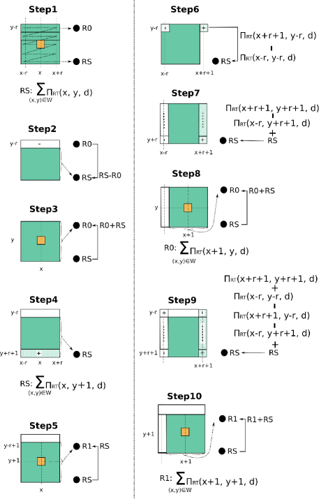
Figure 6: Efficient zigzag scanning

IV-C Implementation of DT

Since DT is performed based on the ZNCC computation results, the task assignment is the same as that of ZNCC shown in Fig.4. In DT, because the cost values must be aggregated in four directions (left to right, right to left, up to down, and down to up), a large memory space is required. The size of on-chip shared memory is too small for this purpose, and we need to use the off-chip global memory. Here, because both the ZNCC ((1)) and weighting operations ($\eqref{equ:k1}$ to ${\eqref{equ:k4}}$) usually generate floating-point cost values (32 bits), there is not only causes a great burden on data transmission, but also a greater requirement for requires more shared-memory space, which reduces the parallelism of multi-thread processing. To solve these problems, it is usually good to use shorter integers (16 bits or even 8 bits) to represent the cost values instead of the floating-point data type. However, a serious problem needs to be addressed here. The magnitude of the aggregated cost values around the boundary of each area decreases due to the use of weight. Hence, the magnitude is sufficiently small for 16-bit integers but not for textureless regions. Figure.7 (a) shows an example of cost aggregation in a large white wall with less texture. Let $P(x^{\prime},y^{\prime})$ be a pixel that belongs to the wall in the image; its cost values $C(x^{\prime},y^{\prime},d)$ are accumulated from all pixels in this area according to (3) to (6). Due to the size of the wall (around 250x300 pixels) and the range of the ZNCC result ([0,1] as mentioned in Section III-A), the accumulated floating-point cost values $C(x^{\prime},y^{\prime},d)$ will largely exceed the upper limit on a 16-bit integer, causing overflow. As such, these cost values cannot be simply converted to integers by multiplying by a coefficient. In [18], we propose a solution to this problem by shifting the matching cost of census to quickly reduce the value range and compressing the 16-bit data into an 8-bit data with a 1-bit flag code. However, the shifting method is not suitable for ZNCC because of its decimal cost value; furthermore, a 1-bit flag code can only specify two positions on a 16-bit integer, which may reduce accuracy.

Therefore, we upgrade the original solution by using a two-step strategy to reduce the aggregated costs’ data width and burden of transmission:

• Use a cost-value normalization with a nearly zero-mean to represent the original floating-point cost values with 16-bit short integers.

• Apply a data encoding & decoding method to further replace the normalized 16-bit short integers with 8-bit by using a 2-bit flag code.

The details of this strategy are as follows:

Cost-value Normalization with Nearly Zero-Mean

Figure.7 (b) shows the change in the cost values of $P(x^{\prime},y^{\prime})$ along the disparity (from 0 to $D-1$). Curve1 represents the change of $C(x^{\prime},y^{\prime},d)$ obtained by (6) (where $C_{D}(x^{\prime},y^{\prime},d)$ is used as final $C(x^{\prime},y^{\prime},d)$ as described above), and $C(x^{\prime},y^{\prime},d_{min})$ shows the minimum value along the curve. The corresponding disparity $d_{min}$ is the result obtained based on the magnitude relationship of $C(x^{\prime},y^{\prime},d)$ according to (15). Therefore, as long as the magnitude relationship remains unchanged, changing the values of $C(x^{\prime},y^{\prime},d)$ will not affect obtaining the correct $d_{min}$. Additionally, since the range of $C(x^{\prime},y^{\prime},d)$ is narrow (as shown in Fig.7, Cost_gap, the difference between the max and min of $C(x^{\prime},y^{\prime},d)$ is much smaller than the values of $C(x^{\prime},y^{\prime},d)$ themselves. Since the range of Cost_gap is narrow, each cost value can be nearly zero-mean normalized by subtracting $C(x^{\prime},y^{\prime},d_{arb})$, where $d_{arb}$ is an arbitrary disparity ($d_{arb}\neq{d_{min}}$). By subtracting the median value, the range of $C(x^{\prime},y^{\prime},d)$ can be minimized; in our implementation, however, an arbitrary value $C(x^{\prime},y^{\prime},d_{arb})$ is used to simplify the calculation. Then (6) can be changed to:

$$C^{\prime}_{D}(x,y,d) =C^{\prime}_{U}(x,y,d)+C^{\prime}_{D}(x,y+1,d)\cdot{W_{D}(x,y)}$$

$$-C^{\prime}_{U}(x,y,d_{arb}),$$ (21)

where $C^{\prime}$ represents the normalized cost value such that the mean approaches zero. This effectively suppresses the increase in the aggregated cost values. To further ensure that these values will not cause an overflow, the cost-value normalization is extended in all directions. At the same time, each accumulated floating-point cost value is scaled up to a 16-bit signed integer via an integer coefficient $T$. The value of $T$ needs to be carefully determined according to the actual situation. The larger the value, the higher the accuracy but also the greater the risk of overflow. This approach not only effectively reduces the burden of data transmission, but facilitates the further reduction of data width using the following method.

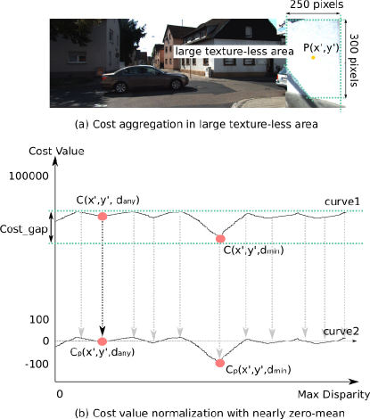
Figure 7: Cost-value normalization with nearly zero-mean

Data Encoding & Decoding

After cost normalization, the value of $C^{\prime}(x^{\prime},y^{\prime},d_{arb})$ is reduced to 0 and some values, including $C^{\prime}(x^{\prime},y^{\prime},d_{min})$, become negative (when $d_{arb}\neq{d_{min}}$). Therefore, it is possible to further reduce the data width by focusing only upon the negative values while ignoring the positive ones. Our method includes two stages: encoding and decoding. Figure.8 shows the process of our method. In the encoding stage, the 16-bit cost value is first compressed into an 8-bit code containing a 6-bit value and a 2-bit flag. This 6-bit value represents the 6 significant bits of the 16-bit integer, and the 2-bit flag shows its position. In the decoding stage, each 8-bit code is decompressed into a 16-bit approximation by putting the 6-bit value in the 16-bit integer on the position specified by the 2-bit flag code. Between the stages, four adjacent 8-bit codes are packed into a 32-bit integer for more efficient transmission on a GPU.

The details of the process in Fig.8 can be described as follows:

• Encoding

  1. As mentioned above, only negative values are used. Therefore, all positive values are set to 0 by checking the sign bit.

  2. Since two’s complement is used to represent the negative values, we first test the 4-bit $Data_{16}[14:11]$ to find whether it is ${}^{\prime}1111^{\prime}$. If not, ($Data_{16}[14:9]$) is chosen as the 6-bit code and ${}^{\prime}01^{\prime}$ is attached to it as the 2-bit flag to show the position of the 6-bit code in the original 16-bit integer. Then, an 8-bit dataset, $Data_{8}$, is constructed from the 16-bit integer.

  3. If $Data_{16}$[14:11] is ${}^{\prime}1111^{\prime}$, the next 4-bit code ($Data_{16}[10:7]$) is checked in the same way. If it is not ${}^{\prime}1111^{\prime}$, $Data_{16}[10:5]$ is chosen as the 6-bit code and the flag code ${}^{\prime}10^{\prime}$ is attached to show its position.

  4. Finally, if $Data_{16}[14:11]$ and $Data_{16}[10:7]$ are both ${}^{\prime}1111^{\prime}$, $Data_{16}[6:1]$ is chosen as the 6-bit code (no checking is necessary) and the 2-bit flag code ${}^{\prime}11^{\prime}$ is attached.

• Decoding

  1. We first check whether $Data_{8}$ is ${}^{\prime}0^{\prime}$ or not. If it is, $Data_{16}$ is also set to ${}^{\prime}0^{\prime}$; if not, its flag code $Data_{8}[1:0]$ is checked.

  2. If the 2-bit flag code is ${}^{\prime}11^{\prime}$, the 6-bit code at $Data_{8}[7:2]$ is copied to $Data_{16}[6:1]$; if the flag code is ${}^{\prime}10^{\prime}$, the 6-bit code is copied to $Data_{16}[10:5]$; if the flag code is ${}^{\prime}01^{\prime}$, the 6-bit code is copied to $Data_{16}[14:9]$.

  3. Then, the bits on the left-hand side of the copied 6-bit code in $Data_{16}$ are set to ${}^{\prime}1^{\prime}$ and the bits on the right side are set to ${}^{\prime}0^{\prime}$.

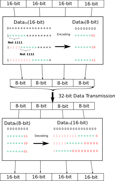
Figure 8: Data encoding & decoding

This method uses the 2-bit flag code, which specifies four position; and the position of the 6-bit code is not continuous on a 16-bit integer. While this is more accurate than the 1-bit flag code which specifies two positions, our approach still loses more information than general 16-bit to 6-bit data-width reduction. However, according to our experiments, high speed processing is possible without losing too much accuracy.

V Evaluation

(a) Regcount = 32

(b) Regcount = 48

(c) Regcount = 60

Figure 9: Processing speed comparison for summation

(a) Regcount=32, $H_{Z}$=32

(b) Regcount=32, $H_{Z}$=64

(c) Regcount=32, $H_{Z}$=128

(d) Regcount=48, $H_{Z}$=32

(e) Regcount=48, $H_{Z}$=64

(f) Regcount=48, $H_{Z}$=128

(g) Regcount=60, $H_{Z}$=32

(h) Regcount=60, $H_{Z}$=64

(i) Regcount=60, $H_{Z}$=128

Figure 10: Processing speed evaluation for Z²-ZNCC

Figure 11: Processing speed comparison for Z²-ZNCC

We implemented our acceleration approach on an embedded GPU Jetson Tx2 and evaluated

1. summation,

2. Z²-ZNCC,

3. FastDT, and

4. the processing speed and matching accuracy of the stereo-matching system based on the Z²-ZNCC, census, semi-global matching (SGM), and FastDT,

algorithms using the KITTI 2015 [5] benchmark.

V-A Evaluation of Summation

The processing speeds of the two summation methods described in Section IV are compared using 1,280x384 pixel images. In our evaluation, the maximum number of registers (Regcount) for each thread is limited to 32, 48, and 60; then comparisons are performed for different window sizes and GPU blocks.

Figure.9 compares the results of the two summation methods. In each graph, M1 and M2 represent the two methods and BS represent the GPU block size. The $x$-axis represents matching windows’ side length from 3 to 15 and the $y$-axis represents their corresponding processing times. In Method 1, each block processes 64 columns and three sets of rows: 16, 8, and 4. As the side length increases, the processing time increases accordingly. This is occurs not only due to the increase in the amount of the calculation, but also to the increase in memory occupancy, which reduces the number of active threads. On the other hand, in Method 2, each block processes three sets of columns: 64, 128, and 256. Because the sum is calculated based on the integral image, the processing time does not change with side length. Here, we note that in all cases, the processing time does not change significantly with the GPU-block size because the parallelism of threads is not affected. For all three different block sizes in Method 2, the processing times for the first two steps of obtaining an integral image is about 355 $\mu{s}$ and 496 $\mu{s}$, respectively, and the total time including the averaging calculation is close to 1.4 ms. Due to the integration, the processing speed of Method 2 is not as fast as that of Method 1 when the window size is smaller than 9x9. Therefore, the methods can be chosen according to actual requirements. However, when BS = 64x16 and Regcount = 48 (or Regcount = 60), Method 1 becomes invalid when the side length is larger than 9 (or 7); this is because the large number of threads causes the number of allocated registers to exceed the allowable upper limit. Therefore, for Method 1, a small GPU block should be chosen so as to ensure that the summation can be performed correctly.

V-B Evaluation of Z²-ZNCC

Figure.10 shows the evaluation results for Z²-ZNCC using the same 1,280x384 size images with a maximum disparity of 128. To show the performance of Z²-ZNCC more clearly, Method 2 is used for the summation because of its consistent processing speed. In addition to Regcount, the evaluation is performed under various $V_{Z}$ and $H_{Z}$ conditions, as described in Section.IV. $V_{Z}$ is changed from 2 to 6 and $H_{Z}$ is set to 32, 64, and 128. A large $V_{Z}$ means that the rate of data reuse is high; however, it also requires a larger Regcount, which will affect the parallelism of threads. Similarly, a large $H_{Z}$ suggests that a large number of $\Pi_{RT}(x,y,d)$ need to be calculated at the same time, which also requires many registers. According to this figure, we note that in most cases, when $V_{Z}$ = 2, Z²-ZNCC performs the worst because of its low data-reuse rate. Furthermore, the larger the side length, the worse the performance, because step 7 in Fig.6 does not work effectively. For $V_{Z}$ = 5 or 6, the performance is still poor when Regcount = 32 (because of the limited number of registers) or when $H_{Z}$ = 128 (because of too much use of registers). Additionally, for the case shown in Fig.10 (c), the larger the $V_{Z}$ value, the worse the performance of Z²-ZNCC, with the exception of $V_{Z}$ = 2. Comparing Figs.10 (f) and (i) with (c), we can see that, by increasing the Regcount to 48 and 60 respectively, the performance can be improved accordingly. However, the difference between (f) and (i) is not large, meaning that increasing Regcount does not improve performance proportionally. For other cases, the processing time increases with the side length without any obvious outliers. The results show that increasing Regcount improves performance more than changing the $H_{Z}$, as shown in Fig.10 (a), (d), and (g). Finally, when $V_{Z}$ = 4, Z²-ZNCC always performs consistently. This means that it achieves a good balance between hardware resources and calculations according to our evaluations.

In addition, we also compared Z²-ZNCC to other methods under various maximum disparity values. Figure.11 shows the results of five methods: two Z²-ZNCC methods, two original progressive-scan methods, and RTNCC [19]. $D$ represents the maximum disparity value and is set to 90, 96 and 128. Based on the summation-speed comparison, we use Method 1 when the window sizes are smaller than 9x9 and Method 2 when the window sizes are larger than 7x7. In the Z²-ZNCC methods, $V_{Z}$ = 4, $H_{Z}$ = 32 and Regcount = 60. The proposed Z²-ZNCC methods work faster than other methods where the disparity is 96 and 128. When the side length is 3 and $D$ = 128, the processing time is 18.05 ms for Original and 11.31 ms for Z²-ZNCC: a 38% increase in speed. When the side length is changed to 15, the processing time is 72.09 ms for Original and 34.35 ms for Z²-ZNCC, meaning that the processing time is reduced by more than half. This is mainly because the Z²-ZNCC methods can reuse data in the vertical direction but the original methods cannot. Furthermore, compared with the latest RTNCC (its $D$ is only 90), our method for $D$ = 96 requires only 16.04 ms, which is 26% faster despite its computational complexity.

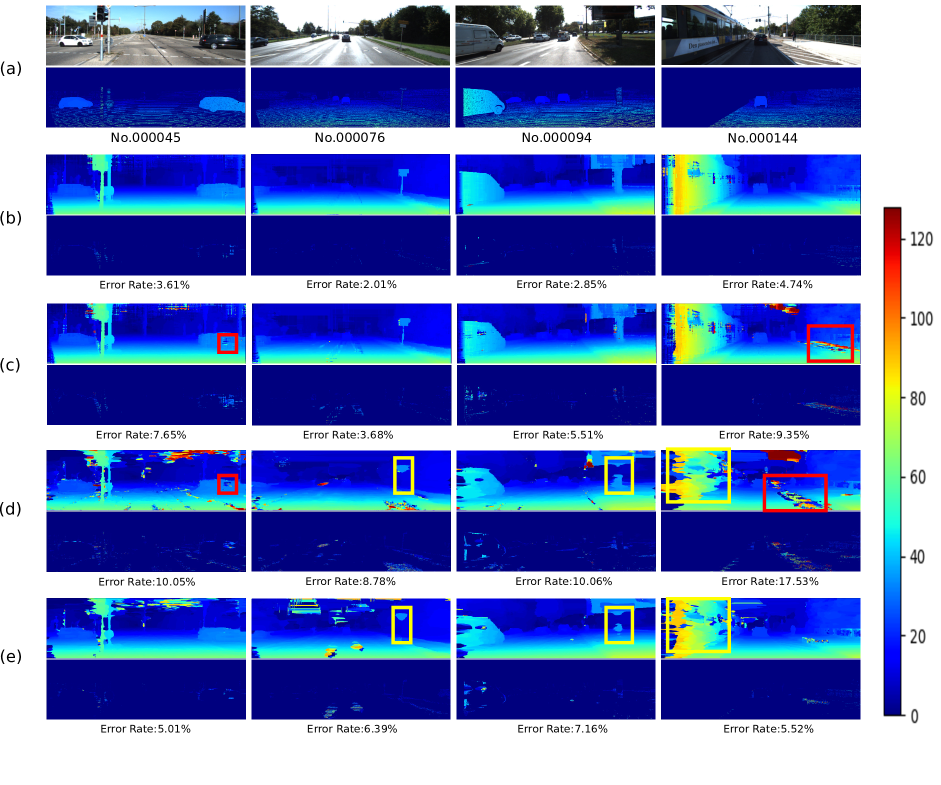
Figure 12: Matching Result(KITTI 2015): (a) Left image & ground truth; (b) S1: Z²-ZNCC+SGM; (c) S2: Census+SGM; (d) S3: Census+FastDT; (e) S4: Z²-ZNCC+FastDT

Figure 13: Comparison with other systems

TABLE I: Comparison of Kernel Performance In Z²ZNCC.

Method	GT(G/s)	GE(%)	IPW	IPC
Original ZNCC	0.92	67.09	1.06e+05	3.05
Z2ZNCC	1.16	76.95	3.06e+05	3.15

• GT: gld_throughput GE: gld_efficiency IPW: inst_per_warp IPC:inst_per_cycle

Table.I shows the comparison between Z²ZNCC and the original ZNCC in terms of kernel performance. We use gld_throughput and gld_efficiency to evaluate the performance of our kernel in memory access, and use inst_per_warp and inst_per_cycle for the computational efficiency. In particular, the number of our IPW is roughly three times the original, which shows that our method can effectively save on-chip resources to maintain a high degree of thread parallelism.

V-C Evaluation of FastDT

We evaluated FastDT in combination with Z²-ZNCC using the training set of the KITTI 2015 [5] benchmark because the accuracy must be evaluated precisely. 200 pairs of images are included in the training set, and their sizes are close to 1,250x375 with a maximum disparity value of 128. In our evaluation, Regcount = 48, T = 21 and the side length of ZNCC is set to 3. The two parameters in (III-B) are $\sigma_{s}$ = 5 and $\sigma_{r}$ = 52. $d_{arb}$ is set to 0 to effectively reduce the range of cost values because $d_{min}$ is rarely equal to zero in stereo matching.

TABLE II: Comparison of DT in KITTI 2015.

Direction	Float	Int32	Int16	Int8 (Ours)	Int16-NP
L2R∗(ms)	13.10	13.76	13.63	13.68	13.59
R2L(ms)	15.41	15.32	8.72	5.52	8.56
U2D(ms)	15.12	15.05	8.74	7.22	8.65
D2U∗(ms)	7.06	7.03	6.29	6.27	6.34
Frame Rate(fps)	20	20	26	32	27
Error Rate(%)	7.36	7.49	7.57	7.63	8.14

• L2R^∗:Z²-ZNCC & left to right. R2L: right to left. U2D: up to down. D2U^∗: down to up & WTA. NP: non-normalization.

Table II shows the processing time for each step of DT under four different methods, together with their accuracy. The four methods–Float, Int32, Int16, and Int8–use floating-point, integer, short integer, and character respectively during cost propagation. Because Z²-ZNCC calculates the cost value for each pixel serially, it is combined with the cost propagation from left to right (L2R). WTA is also combined with the cost propagation from down to up (D2U) to calculate the disparity map directly without transferring cost values back to the global memory. According to our observation, the cost values aggregated during the L2R step are not usually large. Therefore, in our implementation, cost-value normalization is performed only in the U2D steps of Float, Int32, and Int16, and in the R2L step of Int8. The encoding is performed at the end of the R2L step and the decoding is performed at the beginning of the U2D step. Additionally, to verify the necessity of cost-value normalization, we added the evaluation of Int16-NP, in which such normalization is not performed. In the L2R step, the processing time is roughly the same regardless of the data type because the transmission latency is hidden by the calculation time of Z²-ZNCC. On the other hand, the processing time of Int16 is only 8.72 ms in the R2L step and 8.74 ms in the U2D step, which are roughly half of the values for Float and Int32. For Int16-NP, since it is roughly the same as Int16 in terms of calculation and data transmission, there is no obvious difference in processing time. Our Int8 shows the fastest processing speed of all methods, even though data encoding & decoding is performed. This is because our method transfers data in 8-bit, which greatly reduces the latency of data transfer. Table.III shows the comparison between FastDT and the original DT in terms of global memory accessing. As the results of gld_throughput and gld_efficiency shown, our kernel significantly improves the efficiency of global memory access in both R2L and U2D directions. This is mainly benefits from our encoder compression method, which can improve transmission efficiency by bundling data. In our implementation, Int8 achieved the requirement for real-time processing with 32 fps, which is 60% faster than the 20 fps attained by Float.

TABLE III: Comparison of Global Memory Efficiency In DT.

Method		L2R	R2L	U2D	D2U
Original DT	GT(G/s)	0.42	0.56	5.18	38.7
	GE(%)	50.3	20.29	59.39	94.16
FastDT	GT(G/s)	0.41	11	17.08	22.6
	GE(%)	50.13	99.2	88.9	88.9

• GT: gld_throughput GE: gld_efficiency.

TABLE IV: Comparison of matching accuracies in KITTI 2015

Error Rate (%)			D1-bg				D1-fg				D1-all
	S1	S2	S3	S4	S1	S2	S3	S4	S1	S2	S3	S4
All / All	6.60	6.98	15.12	7.77	13.58	17.04	23.56	16.71	7.76	8.66	16.52	9.26
All / Est	6.54	6.82	12.56	7.61	13.54	16.92	22.78	16.52	7.71	8.51	14.24	9.10
Noc / All	5.22	5.48	14.33	6.92	11.38	14.83	21.88	15.01	6.24	7.03	14.48	8.26
Noc / Est	5.20	5.44	11.73	6.87	11.38	14.82	21.38	14.99	6.22	6.99	13.38	8.21

• S1: Z²-ZNCC+SGM. S2: Census+SGM. S3: Census+FastDT. S4: Z²-ZNCC+FastDT.

In the accuracy evaluation, Float has the lowest error rate of 8.16%. As the data width decreases, the error rate gradually increases. Compared with the error rate of 8.37% for Int16, that for Int16-NP is higher (8.81%) because of the overflow of the cost values. This shows that our cost normalization with nearly zero-mean works very effectively. Int8 has an error rate of 8.41%, only a 0.25% loss compared to Float. This means that our method can effectively increase the processing speed even as it maintains a high accuracy in stereo matching.

V-D Evaluation of Stereo Matching

Finally, to further clarify the effectiveness of our Z²-ZNCC and FastDT for stereo matching, we also combined them with the state-of-the-art algorithms SGM and census, respectively. Then, we compared their accuracies and processing speeds on a Jetson Tx2 GPU using the KITTI 2015 benchmark. SGM and census were chosen because the GPU system in [14] uses them and has a good performance (8.66% error rate, 29 fps) under the same conditions. Our implementation of the SGM is almost the same as [14]. The difference is that to clarify the role of Z²-ZNCC, we do not use the stream function. The two parameters in SGM–$P1$ and $P2$–are set to 18 and 185, respectively, because the results of Z²-ZNCC are multiplied by the coefficient $T$.

Figure.12 shows the comparisons of three systems based on use our proposed methods, and one other system [14]. The four systems are Z²-ZNCC+SGM, Census+SGM [14], Census+FastDT and Z²-ZNCC+FastDT; they are expressed as S1, S2, S3, and S4, respectively. Four pairs of images are selected from the training set to clearly show the difference in the results of these systems. Figure.12 (a) shows the reference images and their ground truths. Figures.12 (b) to 12 (e) show the results of S1 to S4, respectively. The top half of each figure shows disparity map and the bottom half the corresponding error image compared with the ground truths. The color bar denotes the disparity range of [0,128), with blue representing the farthest objects and red the closest. As for the four sets of results No.000045, No.000076, No.000094, and No.000144, S1 in Fig.12 (b) shows a clear advantage in terms of accuracy. Its error rates of 3.61%, 2.01%, 2.85%, and 4.75% are obviously lower than those of other systems. Compared with S2 in Fig.12 (c), S1 works better in photometric distortions and weak-pattern areas, as shown by the red boxes in Figs.12 (c) and (d). This means that ZNCC has stronger robustness than census. S3 shows a disadvantage in accuracy. Its error rates are the highest among the four systems. This is because, in addition to the less accurate matching by census, DT also easily causes a fattening effect, making some details disappear, as shown in the yellow boxes in Figs.12 (d) and (e). By replacing census with ZNCC, the accuracy of S4 has been greatly improved, as shown in Fig.12 (e). This means that as long as a high precision is achieved in the cost matching stage, DT will not induce an excessive loss in accuracy. Table IV compares the matching accuracies of the four systems using the testing set of KITTI 2015 benchmark. The result is consistent with the above, and the order of accuracy is S1$>$S2$>$S4$>$S3. The use of ZNCC improves the accuracies of the census-based systems by 0.9% (S1 vs. S2) and 7.26% (S4 vs. S3).

Figure.13 shows a comparison with other systems in terms of processing speed and accuracy. The $x$-axis represents the error rate and the $y$-axis represents the time required for processing in ms; thus, the closer the evaluation results are to the origin, the higher the accuracy and the faster the processing speed. All of the CNN-based systems (AnyNet [11], StereoDNN [12], MADNet [13], and RTS²Net [26]) achieved high accuracy, but had no speeds exceeding 10 fps. RTNCC [19] and our S3 (Census+FastDT) algorithm achieved real-time processing speeds of 46 fps and 35 fps, respectively. However, their error rates are larger than 16%, which also limits their usability. S2 (Census+SGM) [14] and our S1 (Z²-ZNCC+SGM) have almost the same processing speed, but our accuracy is 0.5% lower. This shows that our method plays a significant role in stereo matching. As mentioned above, our S4 (Z²-ZNCC+FastDT) improves the accuracy of S3 from 16.52% to 9.26%. Compared with the systems based on SGM (S1 and S2), S4 still has a 1% lower accuracy, but its processing speed is 17% faster, allowing it to truly achieve real-time processing.

VI Conclusion

In this paper, we proposed an acceleration method for the zero-means normalized cross correlation (ZNCC) template-matching algorithm for stereo vision on an embedded GPU. This method helps us reuse intermediate calculation results efficiently without frequently transferring them among the hierarchy of memories, leading to a higher processing speed. It also helps to improve the matching accuracy because of its stronger robustness. We evaluated our systems based on this method by using the KITTI 2015 benchmark and showed their efficiency. Since the proposed method does not rely upon the GPU experimental architecture, it can be used on different GPUs; furthermore, it is not limited to GPUs and can be used on other hardware platforms like FPGAs.

To further improve out systems’ performance, we are planning to combine it with other cost-aggregation algorithms. This will be done in future work.

References

- [1] Wenqiang Wang, et al: ”Real-Time High-Quality Stereo Vision System in FPGA”. IEEE Transactions on Circuits and Systems for Video Technology. 25(10): 1696-1708 (2015)
- [2] Mohammad Dehnavi, Mohammad Eshghi: ”FPGA based real-time on-road stereo vision system,” Journal of Systems Architecture: Embedded Software Design, 81: 32-43 (2017)
- [3] Xuchong Zhang, Hongbin Sun, Shiqiang Chen, Lin Song, Nanning Zheng: NIPM-sWMF: ”Toward Efficient FPGA Design for High-Definition Large-Disparity Stereo Matching”. IEEE Transactions on Circuits and Systems for Video Technology. 29(5): 1530-1543 (2019)
- [4] Pin-Chen Kuo, et al: ”Stereoview to Multiview Conversion Architecture for Auto-Stereoscopic 3D Displays”. IEEE Transactions on Circuits and Systems for Video Technology. 28(11): 3274-3287 (2018)
- [5] Moritz Menze, Andreas Geiger: ”Object scene flow for autonomous vehiclesm” IEEE Conference on Computer Vision and Pattern Recognition(CVPR), 2015: 3061-3070
- [6] Oscar Rahnama, et al: ”Real-Time Highly Accurate Dense Depth on a Power Budget Using an FPGA-CPU Hybrid SoC,” IEEE Transactions on Circuits and Systems II: Express Briefs, 66-II(5): 773-777 (2019)
- [7] Xuchong Zhang, He Dai, Hongbin Sun, Nan-Ning Zheng: ”Algorithm and VLSI Architecture Co-Design on Efficient Semi-Global Stereo Matching”. IEEE Transactions on Circuits and Systems for Video Technology. 30(11): 4390-4403 (2020)
- [8] Christoph Hartmann, Ulrich Margull: GPUart - An application-based limited preemptive GPU real-time scheduler for embedded systems. Journal of Systems Architecture: Embedded Software Design. 97: 304-319 (2019)
- [9] Sparsh Mittal: A Survey on optimized implementation of deep learning models on the NVIDIA Jetson platform. Journal of Systems Architecture: Embedded Software Design. 97: 428-442 (2019)
- [10] Mustafa U. Torun, Onur Yilmaz, Ali N. Akansu: ”FPGA, GPU, and CPU implementations of Jacobi algorithm for eigenanalysis”. Journal of Parallel and Distributed Computing. 96: 172-180 (2016)
- [11] Yan Wang, et al: ”Anytime Stereo Image Depth Estimation on Mobile Devices,” IEEE International Conference on Robotics and Automation (ICRA), 2019: 5893-5900
- [12] Nikolai Smolyanskiy, Alexey Kamenev, Stan Birchfield: ”On the Importance of Stereo for Accurate Depth Estimation: An Efficient Semi-Supervised Deep Neural Network Approach,” IEEE Conference on Computer Vision and Pattern Recognition Workshops (CVPR), 2018: 1007-1015
- [13] Alessio Tonioni, Fabio Tosi, Matteo Poggi, Stefano Mattoccia, Luigi di Stefano: ”Real-Time Self-Adaptive Deep Stereo,” IEEE Conference on Computer Vision and Pattern Recognition (CVPR), 2019: 195-204
- [14] Daniel Hernández Juárez, et al: ”Embedded Real-time Stereo Estimation via Semi-Global Matching on the GPU,” International Conference on Computational Science (ICCS), 2016: 143-153
- [15] Zhuoyuan Chen, et al: ”A Deep Visual Correspondence Embedding Model for Stereo Matching Costs,” IEEE International Conference on Computer Vision (ICCV), 2015: 972-980
- [16] Qiong Chang, Tsutomu Maruyama: ”Real-Time Stereo Vision System: A Multi-Block Matching on GPU,” IEEE Access 6: 42030-42046 (2018)
- [17] Martin Werner, Benno Stabernack, Christian Riechert: ”Hardware implementation of a full HD real-time disparity estimation algorithm,” IEEE Transactions on Consumer Electronics, 60(1): 66-73 (2014)
- [18] Qiong Chang, Aolong Zha, Masaki Onishi, Tsutomu Maruyama: ”A GPU Accelerator for Domain Transformation-Based stereo Matching,” International Conference on Algorithms, Computing and Artificial Intelligence (ACAI), 2019 (pp. 370-376).
- [19] Cui, Han, and Naim Dahnoun. ”Real-Time Stereo Vision Implementation on Nvidia Jetson TX2,” Mediterranean Conference on Embedded Computing (MECO), 2019. p. 1-5.
- [20] Qiong Chang, et al: Z2-ZNCC: ZigZag Scanning based Zero-means Normalized Cross Correlation for Fast and Accurate Stereo Matching on Embedded GPU. IEEE International Conference on Computer Design (ICCD), 2020: 597-600
- [21] Chuan Lin, Ya Li, Guili Xu, Yijun Cao: ”Optimizing ZNCC calculation in binocular stereo matching. Signal Processing: Image Communication, 52: 64-73 (2017)
- [22] Fan Rui, and Naim Dahnoun. ”Real-time implementation of stereo vision based on optimised normalised cross-correlation and propagated search range on a gpu,” IEEE International Workshop on Imaging Systems and Techniques (IST), 2017:pp.1-6.
- [23] Cuong Cao Pham and JaeWook Jeon. ”Domain Transformation-Based Efficient Cost Aggregation for Local Stereo Matching,” IEEE Transactions on Circuits and Systems for Video Technology, 2013: pp.1119-1130.
- [24] NVIDIA Corporation: ”NVIDIA CUDA C programming guide,” 2019.Version 10.1.243.
- [25] Qiong Chang, Tsutomu Maruyama: ”Real-Time High-Quality Stereo Matching System on a GPU,” IEEE International Conference on Application-specific Systems, Architectures and Processors (ASAP), 2018: 1-8
- [26] Pier Luigi Dovesi, et al: ”Real-Time Semantic Stereo Matching,” IEEE International Conference on Robotics and Automation (ICRA), 2020: 10780-10787.