Constant-Roll Inflation in modified $f(R,\phi)$ gravity model using Palatini Formalism

In this work, we study a constant-roll inflationary model in the Palatini formalism using modified gravity. Here our action consists a non-minimal coupling of a scalar field $\phi$ with Ricci scalar $R$ in a general form of $f(R,\phi)$. Using Palatini approach, we write its equivalent scalar-tensor form in the Einstein frame and then apply the constant-roll condition in the equation of motion for the inflaton field. Later the tensor-to-scalar ratio and the spectral index are calculated using the slow-roll parameters and the results obtained are matched with the Planck 2018 data. We found that the results agree nicely with the observations within the parameter regime under consideration.

I.    Introduction

Inflation [1, 2, 3, 4, 5, 6, 7] is the period of exponential expansion of the universe in the first few instants when it was born. It was first introduced in the 1980s to resolve the problems of the standard Big Bang cosmology like the horizon problem and the flatness or the fine-tuning problem. Not only did it help in resolving these problems, it also provided a mechanism for generating the primordial fluctuations which might have resulted into the large scale structure of the universe that we see today [8, 9, 10, 11, 12, 13]. One other prediction was the scale-invariance of the primordial power spectrum of cosmological fluctuations which has been confirmed in the observation of the Cosmic Microwave Background (CMB) anisotropies [14, 15, 16]. Though inflation provides an excellent description of the early universe, different alternative models have been proposed based on bouncing cosmology [17, 18] which attempt to provide a viable non-singular description of the universe [19]. One such model is of matter-dominated collapsing universe [20, 21] which is succeeded by the non-singular bounce and can act as an alternative to inflation while also explaining the scale-invariance of the primordial power spectrum [22, 22, 23, 24, 25]. Though no one can exclude the possibility of a cyclic evolution of the universe, it is much easier to work and to understand the theory of inflation starting from Big Bang imagining a point-sized universe with an infinite density and temperature with all the fundamental interactions unified by a yet unknown framework.

One of the popular models of the inflation is the Starobinsky model [26] which has an additional $R^{2}$ term in the Einstein-Hilbert action in a pure gravity scenario and is in agreement with the observations in regards to its inflationary spectrum. For other modified gravity models, one can look into [27, 28, 29, 30, 31]. In such models, the scalar degree of freedom (inflaton) arises as the effective scalar degree of freedom induced from the gravity and one can recast the action $\int\mathrm{d}^{4}x\sqrt{-g}f(R)$ as a scalar-tensor theory with a non-minimal coupling of the aforementioned effective scalar degree of freedom with the Ricci Scalar. But this entire analysis works best in the metric formulation of General Relativity (GR). There is another formulation in GR which is widely popular and is known as Palatini formalism which treats the space-time connections as an independent variable [32, 33, 34, 35] while this not the case for the metric approach. Even though both approaches lead to the same equations for the Einstein-Hilbert action, for modified gravity models and the models where the fields are non-minimally coupled to gravity, this statement is not valid. Here, both these formalisms present different physical scenarios. The Starobinsky model, falling under the general category of the $f(R)$ gravity theories, when studied in the Palatini formalism, leads to no inflationary solutions due to the absence of an additional propagating degrees of freedom which is there if we study the system via the metric approach. Hence to study the inflation in Palatini formalism, a scalar field needs to be added to the action and the first such case was studied in [36] where the non-minimal coupling of the scalar field was considered. Since then, many studies have been done considering different inflationary potentials, reheating, post-inflationary phases, preheating and dark matter using $R^{2}$ term in the action [37, 48, 59, 66, 67, 68, 69, 70, 71, 38, 39, 40, 41, 42, 43, 44, 45, 46, 47, 49, 50, 51, 52, 53, 54, 55, 56, 57, 58, 60, 61, 62, 63, 64, 65]. For more detailed review on Palatini formalism, one can look at [72].

Usually, a scalar field, called as ‘inflaton’ drives the exponential expansion of the universe during the inflationary period with the help of an approximately flat potential. This inflaton field slowly rolls down the potential till the minimum is reached thus ending the inflation. This scenario is called slow-roll inflation and one can look at [3, 73, 7, 44, 6] for more details. There are other inflationary solutions as well where this slow-roll condition can be ignored. The ‘ultra slow roll inflation’ [74, 75, 76] is one such scenario in which the curvature perturbation are not frozen at the super Hubble scales thus leading to non-Gaussianities and a more generalized version of that is known as ‘constant-roll inflation’ [77, 78, 79, 80] which consider the rate of acceleration and velocity of the inflaton field as constant. Even though the constant roll models seem to be close to the slow roll ones but these models help us in calculating the slow roll parameters more precisely. Also, another important prediction of the constant roll inflation is the presence of larger non-Gaussianities [81] in the bispectrum than the ones predicted by the ultra-slow roll case.

In this paper, we are exploring the constant roll inflation via Palatini formalism when the Einstein-Hilbert action has an additional $R^{2}$ term non-minimally coupled with a scalar field where $R$ is Ricci scalar. We begin by first finding the scalar field equation for action given in [82] in Sec.II.. Then we proceed to find slow roll parameters in Sec.III. using the constant-roll condition. In Sec.III.A., we plot our results obtained for the spectral index $(n_{s})$ and tensor-to-scalar ratio $(r)$ and do a comparison with the Planck data [16]. Finally, we conclude with Sec.IV. and summarize our findings with the future direction.

II.    $R^{2}$ coupled gravity in the Palatini formalism

We start with the following action[82],

$$S = \int\mathrm{d}^{4}x\sqrt{-g}\left[\frac{1}{2}f(R,\phi)-\frac{1}{2}g^{\mu\nu}\partial_{\mu}\phi\partial_{\nu}\phi-V(\phi)\right],$$ (2.1)

where $g_{ab}$ and $g$ are the metric and its determinant respectively, $f(R,\phi)=G(\phi)(R+\alpha R^{2})$[83] and $\alpha$ is constant. Here $R$ is the Ricci scalar, which is defined as $R=g^{ab}R^{c}_{abc}(\Gamma,\partial\Gamma)$ in the Palatini formalism and we assumed the Planck mass to be 1. This action (2.1) can be equivalently expressed in terms of an auxiliary field $\chi$ as,

$$S = \int\mathrm{d}^{4}x\sqrt{-g}\left[\frac{1}{2}f(\chi,\phi)+\frac{1}{2}\ f^{\prime}(\chi,\phi)(R-\chi)\ -\frac{1}{2}g^{\mu\nu}\partial_{\mu}\phi\partial_{\nu}\phi-V(\phi)\right]\ ,$$ (2.2)

where $f^{\prime}(\chi,\phi)=\frac{\partial f(\chi,\phi)}{\partial\chi}$, satisfying $\chi=R$ on-shell. Thus we can rewrite eq.(2.2) as,

$$S = \int\mathrm{d}^{4}x\sqrt{-g}\left[\frac{1}{2}f^{\prime}(\chi,\phi)R-W(\chi,\phi)-\frac{1}{2}g^{\mu\nu}\partial_{\mu}\phi\partial_{\nu}\phi-V(\phi)\right]\ ,$$ (2.3)

where $W(\chi,\phi)=\frac{1}{2}\chi f^{\prime}(\chi,\phi)-\frac{1}{2}f(\chi,\phi)$. Now using the conformal transformation

$$g_{\mu\nu}\rightarrow f^{\prime}(\chi,\phi)g_{\mu\nu}\ ,$$ (2.4)

action (2.3) can be written in Einstein frame as

$$S = \int\mathrm{d}^{4}x\sqrt{-g}\left[\frac{1}{2}R-\frac{1}{2}\frac{\partial_{\mu}\phi\partial^{\mu}\phi}{f^{\prime}(\chi,\phi)}-\frac{W(\chi,\phi)+V(\phi)}{f^{\prime}(\chi,\phi)^{2}}\right]\ .$$ (2.5)

Now defining a new potential $\hat{V}(\chi,\phi)$ as

$$\hat{V}(\chi,\phi)\equiv\frac{W(\chi,\phi)+V(\phi)}{f^{\prime}(\chi,\phi)^{2}},$$ (2.6)

and by using $f(R,\phi)=G(\phi)(R+\alpha R^{2})$, the above equation can be written as

$$\hat{V}(\chi,\phi)=\frac{1}{f^{\prime}(\chi,\phi)^{2}}\left[\frac{1}{8\alpha G(\phi)}[f^{\prime}(\chi,\phi)-G(\phi)]^{2}+V(\phi)\right].$$ (2.7)

Now varying the action (2.5) with respect $\chi$, we get

$$f^{\prime}(\chi,\phi)=\frac{8\alpha V(\phi)+G(\phi)}{1-2\alpha\partial_{\mu}\phi\partial^{\mu}\phi}.$$ (2.8)

Inserting equation (2.8) into equation (2.7), $\chi$ could be eliminated. And then substituting equation (2.7) into equation (2.5) and simplifying, we obtain

$$S=\int\,d^{4}x\sqrt{-g}\left[\frac{R}{2}-\frac{1}{2}\frac{1}{(8\alpha V+G)}\partial^{\mu}{\phi}\partial_{\mu}{\phi}+\frac{\alpha}{2}\frac{1}{(8\alpha V+G)}(\partial^{\mu}{\phi}\partial_{\mu}{\phi})^{2}-\frac{V}{G(8\alpha V+G)}\right],$$ (2.9)

with the effective Lagrangian [40]

$$\mathcal{L}(\phi,X)\equiv A(\phi)X+B(\phi)X^{2}-U(\phi),$$ (2.10)

where

$$X\equiv\frac{(\nabla{\phi})^{2}}{2}\quad and\quad\begin{cases}A(\phi)\equiv\frac{1}{G(\phi)+8\alpha V(\phi)}=\frac{1}{G(\phi)}\left(1+8\alpha\frac{V(\phi)}{G(\phi)}\right)^{-1},\\ B(\phi)\equiv\frac{2\alpha}{G(\phi)+8\alpha V(\phi)}=\frac{2\alpha}{G(\phi)}\left(1+8\alpha\frac{V(\phi)}{G(\phi)}\right)^{-1},\\ U(\phi)\equiv\frac{V(\phi)}{G(\phi)(G(\phi)+8\alpha V(\phi))}=\frac{V(\phi)}{G(\phi)^{2}}\left(1+8\alpha\frac{V(\phi)}{G(\phi)}\right)^{-1}\end{cases}.$$ (2.11)

Here $\mathcal{L}$ contains up to quartic kinetic terms with field-depended coefficients, which belong to k-inflation models and $U(\phi)$ is the effective potential. By varying the action with respect to metric $g_{\mu\nu}$, the energy momentum tensor of the source field $\phi$ is written as,

$$T_{\mu\nu}=-\frac{2}{\sqrt{-g}}\frac{\delta S}{\delta g^{\mu\nu}}=-(A+2BX)\nabla_{\mu}\phi\nabla_{\nu}\phi+g_{\mu\nu}(AX+2BX-U).$$ (2.12)

Our choice of the background metric is a spatially flat FLRW metric, also the scalar field $\phi$ to be spatially homogeneous, which depends only on time $\phi(t)$. Thus we can get the energy density and pressure from the energy-momentum tensor as

$$\rho=T_{00}=AX+3BX^{2}+U$$ (2.13)

$$p=T_{ii}=AX+BX^{2}-U.$$ (2.14)

Einsteins’ equations of motion are

$$3H^{2}=\rho$$ (2.15)

$$\dot{\rho}+3H(\rho+p)=0$$ (2.16)

where dot represents the derivative with respect to the cosmic time and H is the Hubble parameter. Using eq.(2.15) and eq.(2.16), we get

$$2\dot{H}+3H^{2}=-p.$$ (2.17)

This leads us to the scalar field equation

$$\ddot{\phi}(A+6BX)+3H\dot{\phi}(A+2BX)-A^{\prime}X-3B^{\prime}X^{2}-U^{\prime}=0$$ (2.18)

where prime denotes the derivative with respect to $\phi$.

III.    Constant roll Inflation

The inflaton field $\phi$ is the only degree of freedom that we have in this model. We assume that field $\phi$ satisfies the constant roll condition as

$$\ddot{\phi}=\beta H\dot{\phi},$$ (3.1)

where $\beta$ is the constant roll parameter. And this condition is about the same as the slow roll condition where $\ddot{\phi}\simeq 0$ if $\beta\ll 1$. We also assume that the field $\phi$ satisfies $\frac{{\dot{\phi}}^{2}}{2}\ll U(\phi)$ during the initial phase of the inflation. For that phase, we are defining slow roll parameters as [84],

$$\epsilon_{1}=-\frac{\dot{H}}{H^{2}},\quad\epsilon_{2}=-\frac{\ddot{\phi}}{H\dot{\phi}},\quad\epsilon_{3}=\frac{\dot{F}}{2HF},\quad\epsilon_{4}=\frac{\dot{E}}{2HE}$$ (3.2)

where

$$F=\frac{\partial\mathcal{L}}{\partial R},\quad E=-\frac{F}{2X}\left(X\frac{\partial\mathcal{L}}{\partial X}+2X^{2}{\frac{\partial^{2}\mathcal{L}}{\partial X^{2}}}\right).$$ (3.3)

As we can see, constant roll condition fixes $\epsilon_{2}=-\beta$. And we are working in Einstein frame where $F=\frac{1}{2}$, from which we get $\epsilon_{3}=0$. We may express observable quantities like the scalar spectral index $n_{s}$ and the tensor to scalar ratio r in terms of the slow roll parameters as [73, 85, 86]

$$n_{s}=1-2\frac{(2\epsilon_{1}-\epsilon_{2}-\epsilon_{3}+\epsilon_{4})}{1-\epsilon_{1}}$$ (3.4)

$$r=4|\epsilon_{1}|C_{s}$$ (3.5)

where $C_{s}$ is the speed of sound wave of primordial perturbations, expressed by

$$C_{s}^{2}=\frac{\mathcal{L}_{X}}{\mathcal{L}_{X}+2X\mathcal{L}_{XX}}=\frac{A-B{\dot{\phi}}^{2}}{A-3B{\dot{\phi}}^{2}},$$ (3.6)

which follows, $0<C_{s}^{2}<1$. The scalar power spectrum up to first order in slow-roll parameters is expressed as [5],

$$P_{s}\approx\frac{H^{2}}{8\pi^{2}\epsilon_{1}},$$ (3.7)

Inserting constant roll condition into eq.(2.9) and we obtain

$$4H\dot{\phi}A(\beta+3)-12H\dot{\phi}^{3}B(\beta+1)+A^{\prime}\dot{\phi}^{2}-3B^{\prime}\dot{\phi}^{4}-4U^{\prime}=0$$ (3.8)

Using eq.(2.4) and eq.(2.6), we obtain an approximate result of H upto second order in terms of $\dot{\phi}^{2}/2U$ as

$$H=\sqrt{\frac{U}{3}\left(1-A\left(\frac{\dot{\phi}^{2}}{2U}\right)+3BU\left(\frac{\dot{\phi}^{2}}{2U}\right)^{2}\right)}\approx\sqrt{\frac{U}{3}}\left(1-\frac{A}{2}\left(\frac{\dot{\phi}^{2}}{2U}\right)+\frac{1}{2}\left(3BU-\frac{A^{2}}{4}\right)\left(\frac{\dot{\phi}^{2}}{2U}\right)^{2}\right)$$ (3.9)

Next, we substitute this approximated result of H into eq.(3.8), we get

$$\frac{1}{2}A^{\prime}\dot{\phi}^{2}+(\beta+3)A\sqrt{\frac{U}{3}}\dot{\phi}-U^{\prime}=0,$$ (3.10)

keeping only terms up to $O\left(\dot{\phi}^{2}\right)$ as higher power terms are negligible. Now the eq.(3.10) is a quadratic equation of $\dot{\phi}$, and the solutions of this equation are :

$$\dot{\phi}=\begin{cases}\frac{-\sqrt{2A^{\prime}U^{\prime}+\frac{1}{3}(\beta+3)^{2}A^{2}U}-(\beta+3)A\sqrt{\frac{U}{3}}}{A^{\prime}},\\ \frac{\sqrt{2A^{\prime}U^{\prime}+\frac{1}{3}(\beta+3)^{2}A^{2}U}-(\beta+3)A\sqrt{\frac{U}{3}}}{A^{\prime}}\end{cases}$$ (3.11)

Here, the first solution leads us to an unsolvable set of equations hence we proceed further with the calculation for the second solution of $\dot{\phi}$, which is given by

$$\dot{\phi}=\frac{\sqrt{2A^{\prime}U^{\prime}+\frac{1}{3}(\beta+3)^{2}A^{2}U}-(\beta+3)A\sqrt{\frac{U}{3}}}{A^{\prime}}.$$ (3.12)

This equation can be solved by using eq.(2.11) with the choice of potential and coupling function. As we can see, the scalar spectral index, tensor-to-scalar ratio and the scalar power spectrum, are all just the functions of the slow roll parameters as expressed in equations (3.4), (3.5) and (3.7). So first we need to solve the slow roll parameters from the eq.(3.2). By using the relations (2.11), the general expression (3.2) can be simplified as

$$\epsilon_{1}=\frac{3XA+6X^{2}B}{XA+3X^{2}B+U}=\frac{6\gamma\left(\gamma{\dot{\phi}}^{4}\epsilon-4\delta{\dot{\phi}}^{2}\right)}{16\delta^{2}\phi+\gamma{\dot{\phi}}^{2}\left(3\gamma{\dot{\phi}}^{2}\epsilon-8\delta\right)}$$ (3.13)

$$\epsilon_{2}=-\beta$$ (3.14)

$$\epsilon_{3}=0$$ (3.15)

$$\epsilon_{4} =\frac{\sqrt{3}}{2}\frac{\dot{\phi}(A^{\prime}+6B^{\prime}X)+12\beta BHX}{(A+6BX)\sqrt{AX+3BX^{2}+U}}$$

$$=\frac{\gamma\dot{\phi}\left(3\beta\dot{\phi}\epsilon\sqrt{\phi}\sqrt{\epsilon\phi+1}\sqrt{16\delta^{2}\phi+\gamma\dot{\phi}^{2}\left(3\gamma\dot{\phi}^{2}\epsilon-8\delta\right)}+4\sqrt{3}\sqrt{\delta}\epsilon\phi\left(4\delta-3\gamma\dot{\phi}^{2}\epsilon\right)+2\sqrt{3}\sqrt{\delta}\left(4\delta-3\gamma\dot{\phi}^{2}\epsilon\right)\right)}{\sqrt{\phi}\sqrt{\epsilon\phi+1}\left(3\gamma\dot{\phi}^{2}\epsilon-4\delta\right)\sqrt{16\delta^{2}\phi+\gamma\dot{\phi}^{2}\left(3\gamma\dot{\phi}^{2}\epsilon-8\delta\right)}},$$ (3.16)

similarly, the speed of sound wave of primordial perturbations can be obtained from (3.6) as

$$C_{s}^{2}=\frac{A-B{\dot{\phi}}^{2}}{A-3B{\dot{\phi}}^{2}}=\frac{\gamma{\dot{\phi}}^{2}\left(\gamma{\dot{\phi}}^{2}\epsilon-8\delta\right)-16\delta^{2}\phi(t)}{\gamma{\dot{\phi}}^{2}\left(\gamma\left({\dot{\phi}}^{2}-8\right)\epsilon-8\delta\right)-16\delta^{2}\phi(t)}$$ (3.17)

and scalar power spectrum from the eq.(3.7)

$$P_{s}\approx\frac{H^{2}}{8\pi^{2}\epsilon_{1}}=\frac{1}{72\pi^{2}}\frac{(AX+3BX^{2}+U)^{2}}{AX+2BX^{2}}=\frac{\left(16\delta^{2}\phi+\gamma\dot{\phi}^{2}\left(3\gamma\dot{\phi}^{2}\epsilon-8\delta\right)\right)^{2}}{2304\pi^{2}\gamma^{3}\delta\dot{\phi}^{2}\phi(\epsilon\phi+1)\left(\gamma\dot{\phi}^{2}\epsilon-4\delta\right)}.$$ (3.18)

Here all the slow roll parameters, speed of sound wave and the scalar power spectrum are the function of $\dot{\phi}$, which can be solved by using eq.(3.12) for our choice the potential $V(\phi)$ and coupling function $G(\phi)$. Then, this $\dot{\phi}$ can be substituted back to these expressions of $\epsilon$’s, $C_{s}$ and $P_{s}$.

A.    Results

Our choice of the potential $V(\phi)$ and coupling function $G(\phi)$ is

$$V(\phi)=\delta\phi^{2},\quad G(\phi)=\gamma\phi,$$ (3.19)

even though there are other choices for the potential [82] but we have chosen this for simplicity as it leads to a close set of equations and give viable results. Also, we assume $\epsilon=\frac{8\alpha\delta}{\gamma}\ll 1$ in the effective potential term eq.(2.11), $8\alpha\frac{V(\phi)}{G(\phi)}=8\alpha\frac{\delta}{\gamma}\phi$.

By using eq.(3.19) and eq.(2.11), we get the solution of eq.(3.12) in the power series of $\epsilon$,

$$\dot{\phi}=-\gamma\epsilon\phi^{2}\left(\frac{\sqrt{3}(\beta+3)\sqrt{\delta}}{2\gamma^{2}}-\frac{\sqrt{3}\sqrt{\delta}\left(-2\gamma+\beta^{2}\phi+6\beta\phi+9\phi\right)}{2(\beta+3)\gamma^{2}\phi}\right).$$ (3.20)

Here we ignored the higher power of $\epsilon$ as they are very small since $\epsilon\ll 1$. As a result of the preceding analysis, we get the solution for $\dot{\phi}[\phi]$, depending on $\phi$ and this can be inserted into all the expressions of the slow roll parameters and the number of e-folds.

The number of e-folds can be calculated from the time when a mode k crosses the horizon until inflation ends and is written as

$$N=\int_{\phi_{k}}^{\phi_{f}}\frac{H}{\dot{\phi}}\,d{\phi}={\frac{1}{\sqrt{3}}}{\int_{\phi_{k}}^{\phi_{f}}\frac{\sqrt{XA+3X^{2}B+U}}{\dot{\phi}}\,d{\phi}},$$ (3.21)

where $\phi_{k}$ and $\phi_{f}$ are the values of inflaton field $\phi$ at the horizon crossing and at the end of the inflation, respectively. Since $\phi_{k}\gg\phi_{f}$ during the inflation, we get approximated result of the above equation,

$$N\approx-\frac{\left(\frac{2(\beta+3)^{2}}{\gamma\epsilon}+3\right)\log(\phi_{f}/\phi_{k})}{6(\beta+3)},$$ (3.22)

then $\phi_{k}$ can be obtained as

$$\phi_{k}\approx\phi_{f}\cdot e^{\frac{6(\beta+3)\gamma N\epsilon}{2(\beta+3)^{2}+3\gamma\epsilon}}.$$ (3.23)

We can solve the field value $\phi_{f}$ at the end of the inflation by demanding the condition $\epsilon_{1}(\phi_{f})=1$. Up to first order in $\epsilon$, we get

$$\phi_{f}=\frac{1}{\epsilon}$$ (3.24)

This is value of field $\phi$ at end of the inflation depending on $\epsilon$ and we know $\epsilon={8\alpha\delta}/{\gamma}$. By putting the value of $\phi_{f}$ and N (range of 50-70) into eq.(3.23), the value of $\phi_{k}$ can be obtained. Putting this value into equations (3.13), (3.14), (3.15) and (III.), the slow roll parameters can be calculated in terms of N, $\beta$ and coupling parameters.

$$\epsilon_{1}=-\frac{9\gamma\epsilon}{8(\beta+3)^{2}}+\frac{27\gamma^{2}\epsilon^{2}(16\beta N+48N+31)}{128(\beta+3)^{4}}$$ (3.25)

$$\epsilon_{2}=-\beta$$ (3.26)

$$\epsilon_{3}=0$$ (3.27)

$$\epsilon_{4}=\frac{9\epsilon\left(-\beta\gamma+2\sqrt{2}\beta\gamma+6\sqrt{2}\gamma\right)}{16(\beta+3)^{2}}+\frac{9\epsilon^{2}\left(87\beta\gamma^{2}+2\sqrt{2}(\beta+3)\gamma(-45\gamma-28\beta\gamma N-84\gamma N)\right)}{256(\beta+3)^{4}}.$$ (3.28)

Finally, the scalar spectral index and the tensor-to-scalar ratio are obtained by substituting eq.(3.25) - (3.28) into eq.(3.4) and eq.(3.5)

$$r=4\left(1-\frac{3\gamma^{2}\epsilon^{2}}{16\left((\beta+3)^{2}\delta\right)}+\frac{9\gamma^{3}\epsilon^{3}(8\beta N+24N+17)}{128(\beta+3)^{4}\delta}\right)\Bigg{|}\frac{27(16\beta N+48N+31)\gamma^{2}\epsilon^{2}}{128(\beta+3)^{4}}-\frac{9\gamma\epsilon}{8(\beta+3)^{2}}\Bigg{|}$$ (3.29)

$$n_{s}= 1-2\beta-\frac{9(3\beta+4)\gamma\epsilon}{8(\beta+3)^{2}}-\frac{9\gamma\epsilon}{2\sqrt{2}(\beta+3)}+\frac{63\gamma^{2}\epsilon^{2}(4(\beta+3)N+9)}{32\sqrt{2}(\beta+3)^{3}}$$ (3.30)

$$-\frac{27\gamma^{2}\epsilon^{2}\left(109\beta+32\left(\beta^{2}+5\beta+6\right)N+148\right)}{128(\beta+3)^{4}}$$

and speed of sound is given by

$$C_{s}=\left(1-\frac{3\gamma^{2}\epsilon^{2}}{16\left((\beta+3)^{2}\delta\right)}+\frac{9\gamma^{3}\epsilon^{3}(8\beta N+24N+17)}{128(\beta+3)^{4}\delta}\right)$$ (3.31)

which shall follow the condition,

$$0<C_{s}<1.$$ (3.32)

Now, to match our results with the observations, we choose $\epsilon=10^{-7}$ with $0.006<\beta<0.018$ and the number of e-folds($N$) from 50 to 70 satisfying $\epsilon=8\frac{\alpha\delta}{\gamma}\ll 1$ condition. For this parameter regime, eq.(3.32) implies $\delta$ must be much greater than $10^{-5}$ and hence we choose $\delta=1$. With the fixed values of $\epsilon$ and $\delta$, the only remaining parameters are $N$, $\beta$ and $\gamma$. Then in Fig.$1$, we fix $\gamma=2.5\times 10^{5}$ while varying $\beta$ and $N$ within the allowed range and plot $r$ vs $n_{s}$ results using eq.(3.30) and eq.(3.29). Here, we also notice that as we vary $N$ from $50$ to $70$, the value of $r$ increases while increasing $\beta$ lead to a smaller value of $n_{s}$. Then in Fig.$2$, we overlap our analytical results over Planck 2018 data and show that the results are well in agreement with the observation. Following the same procedure as Fig.$1$, we make Fig.$3$, Fig.$5$, Fig.$7$ and Fig.$9$ for different values of $\gamma$ as shown. Accordingly, all these figures are then overlapped just like Fig.$2$ over the Planck data as shown in Fig.$4$, Fig.$6$, Fig.$8$ and Fig.$10$. With this comparison with the observation, we find that an increased value of $\gamma$ lead to mismatching with the observations thus constraining this parameter as well.

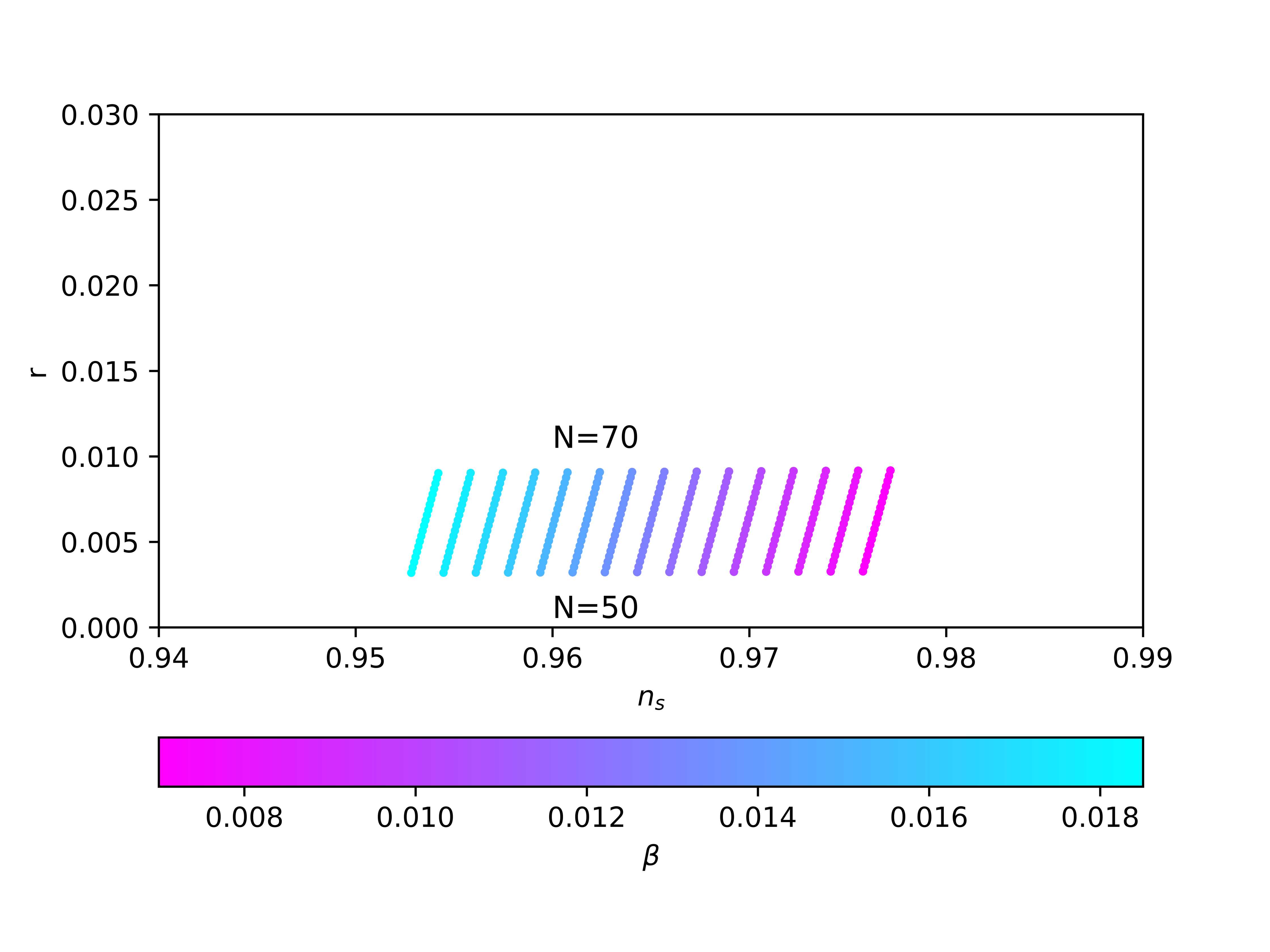
Figure 1: $\gamma=2.5\times 10^{5}$

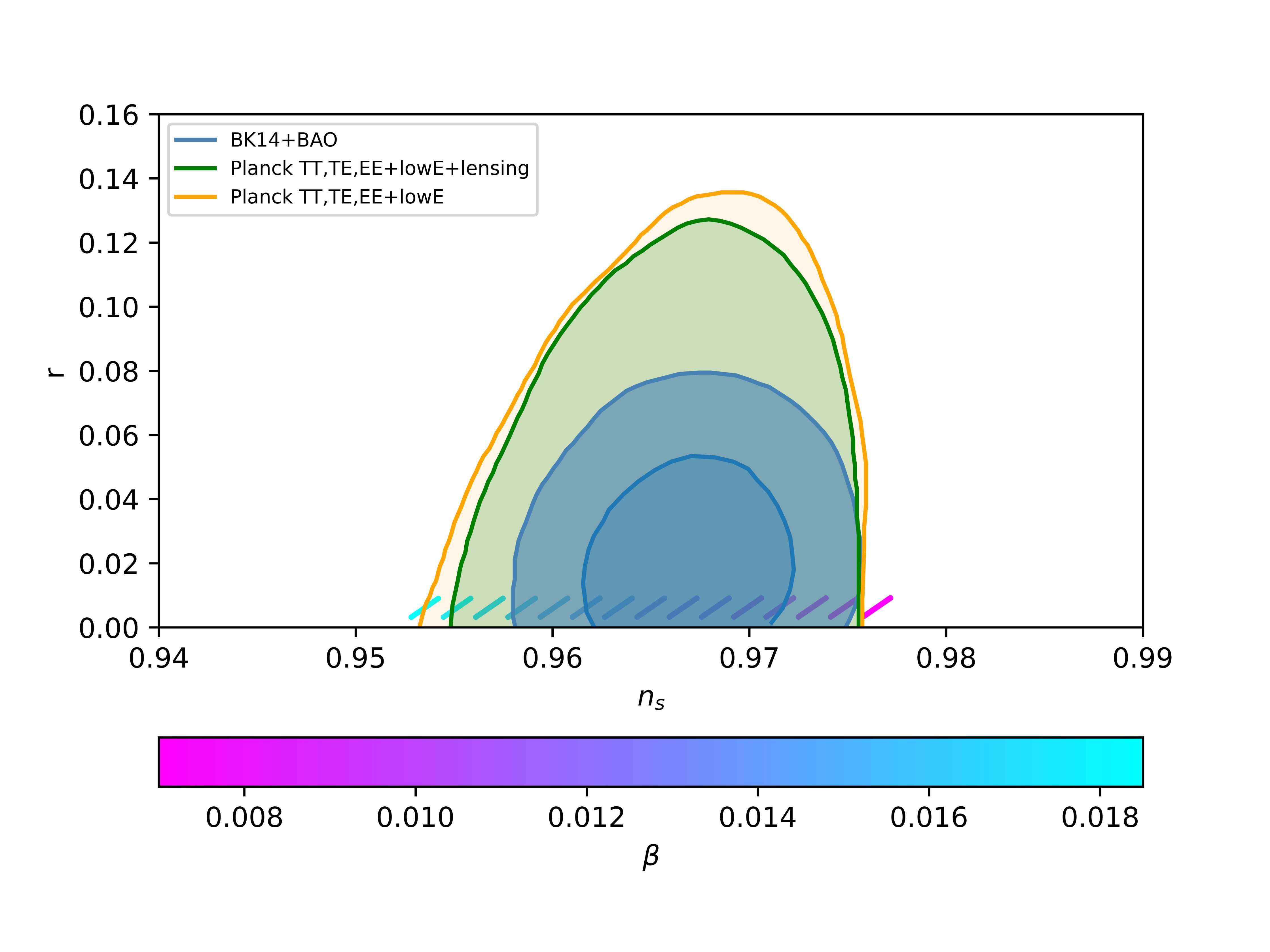
Figure 2: $\gamma=2.5\times 10^{5}$

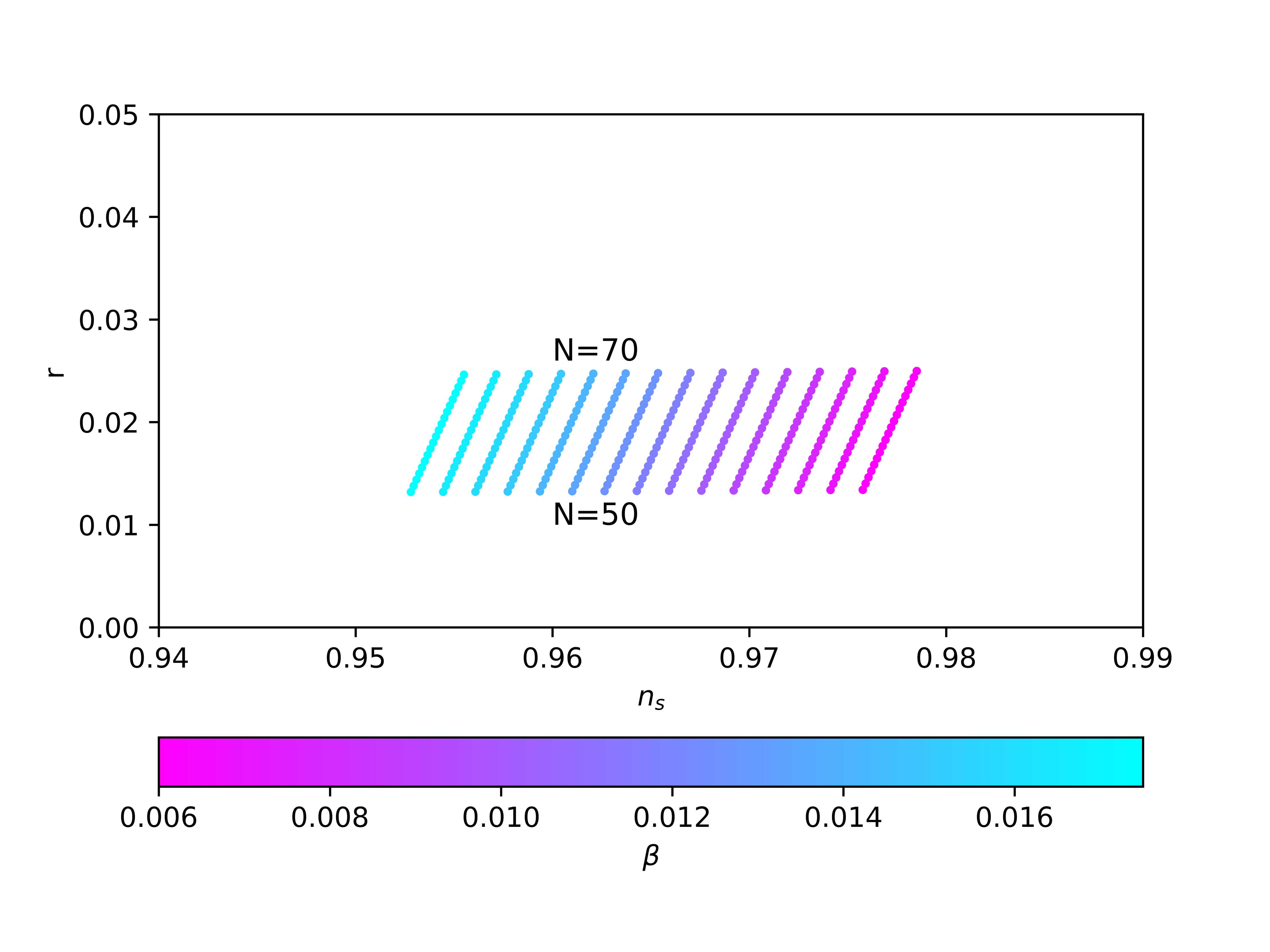
Figure 3: $\gamma=3.5\times 10^{5}$

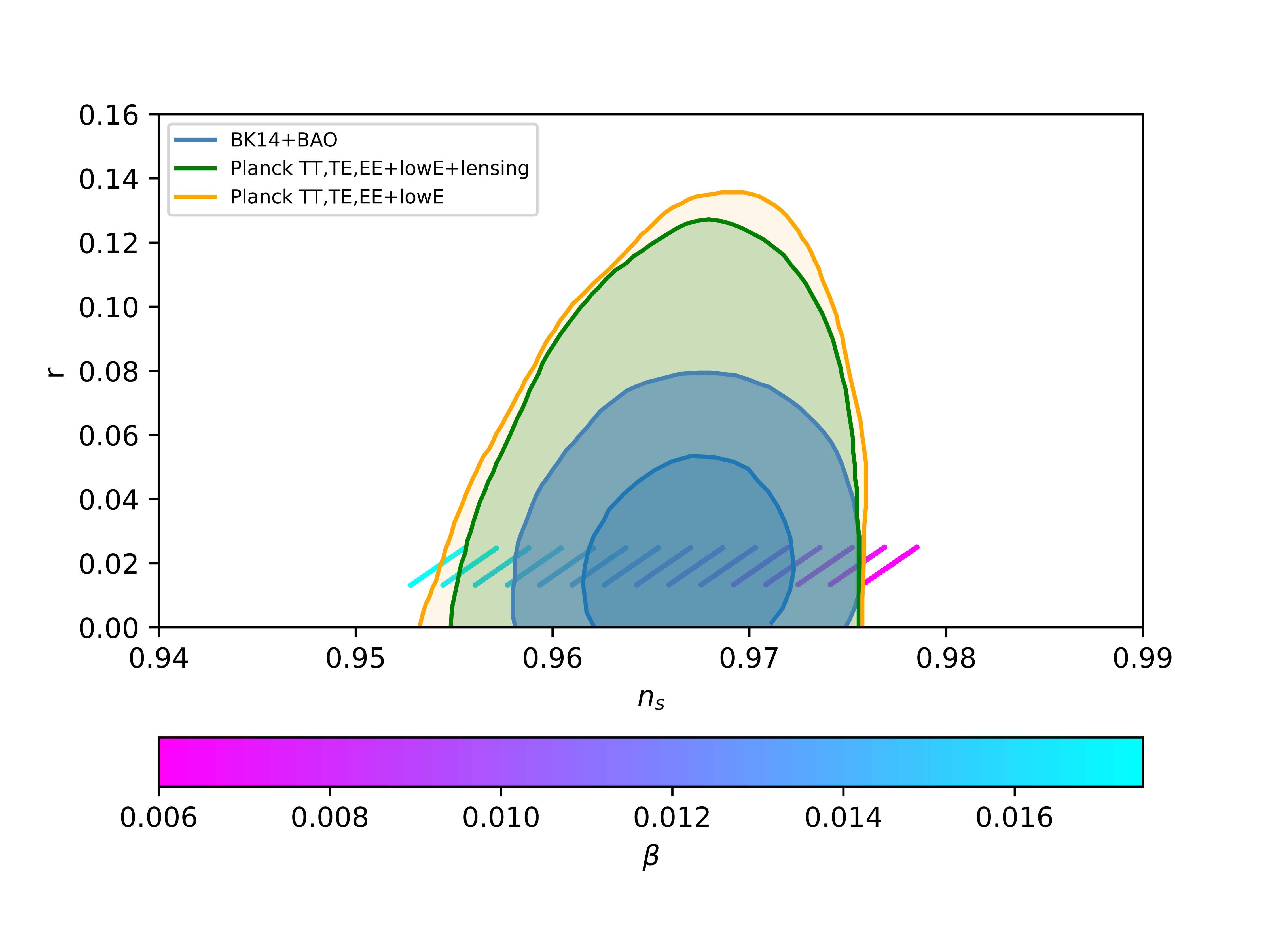
Figure 4: $\gamma=3.5\times 10^{5}$

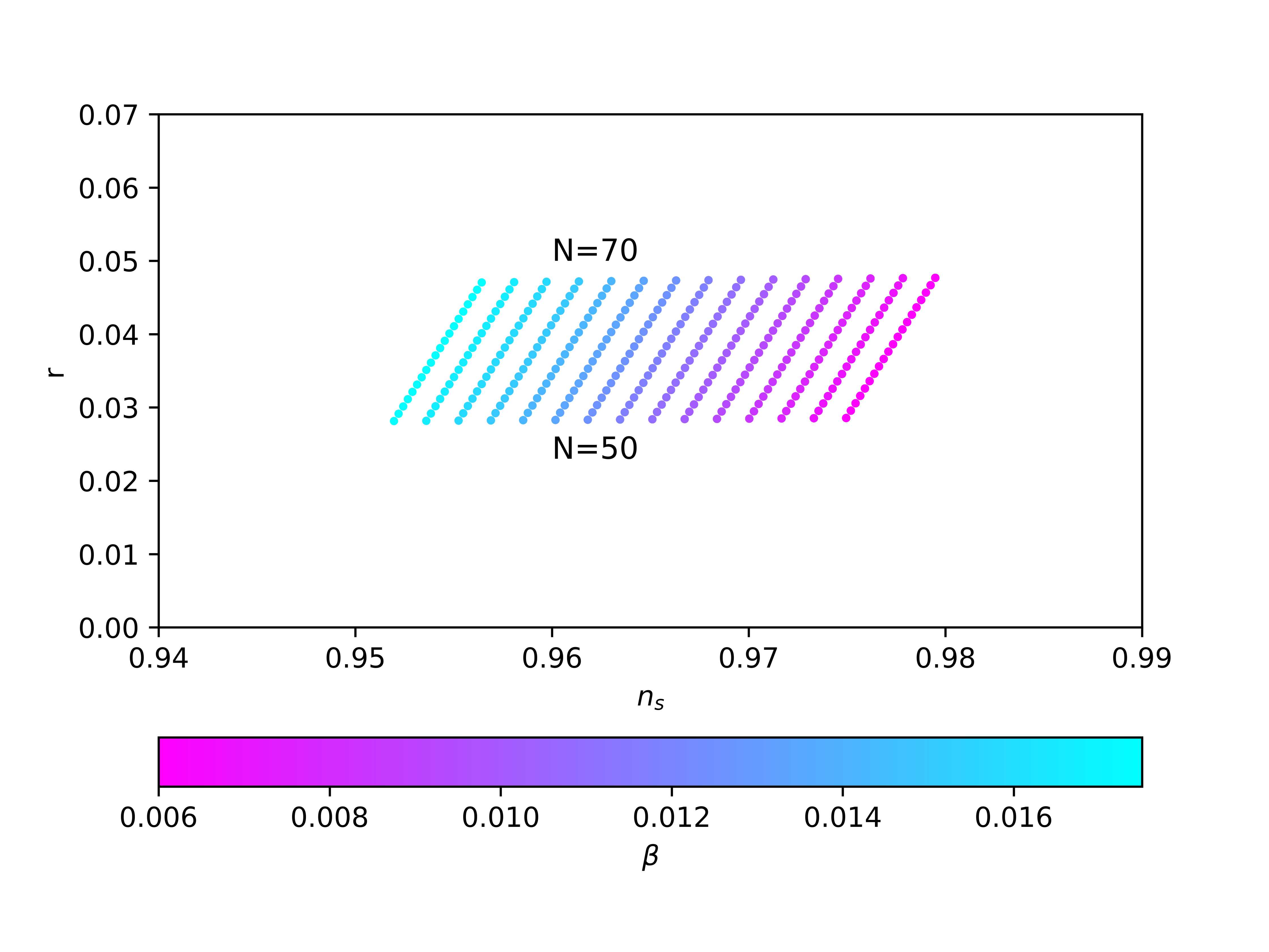
Figure 5: $\gamma=4.5\times 10^{5}$

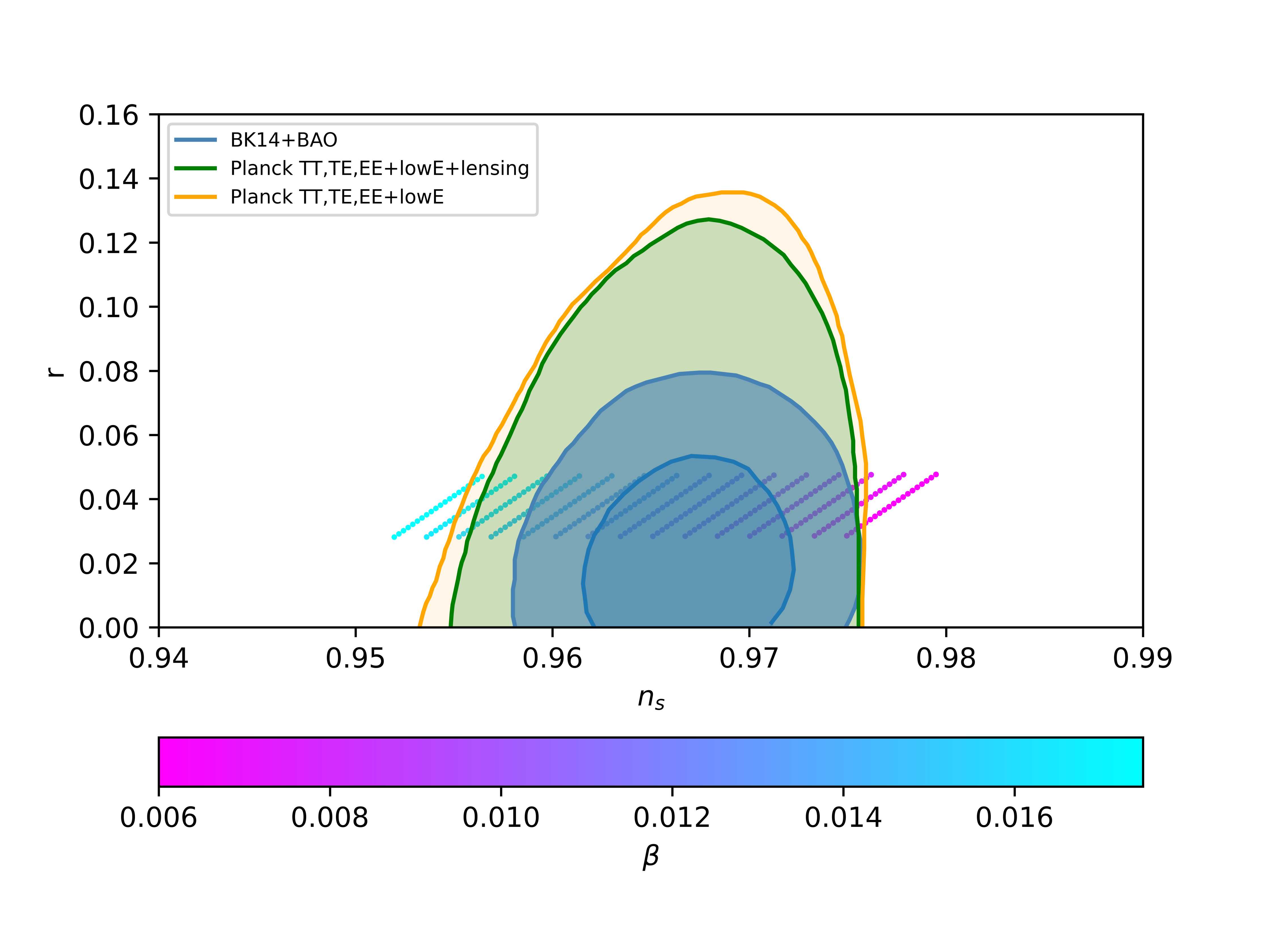
Figure 6: $\gamma=4.5\times 10^{5}$

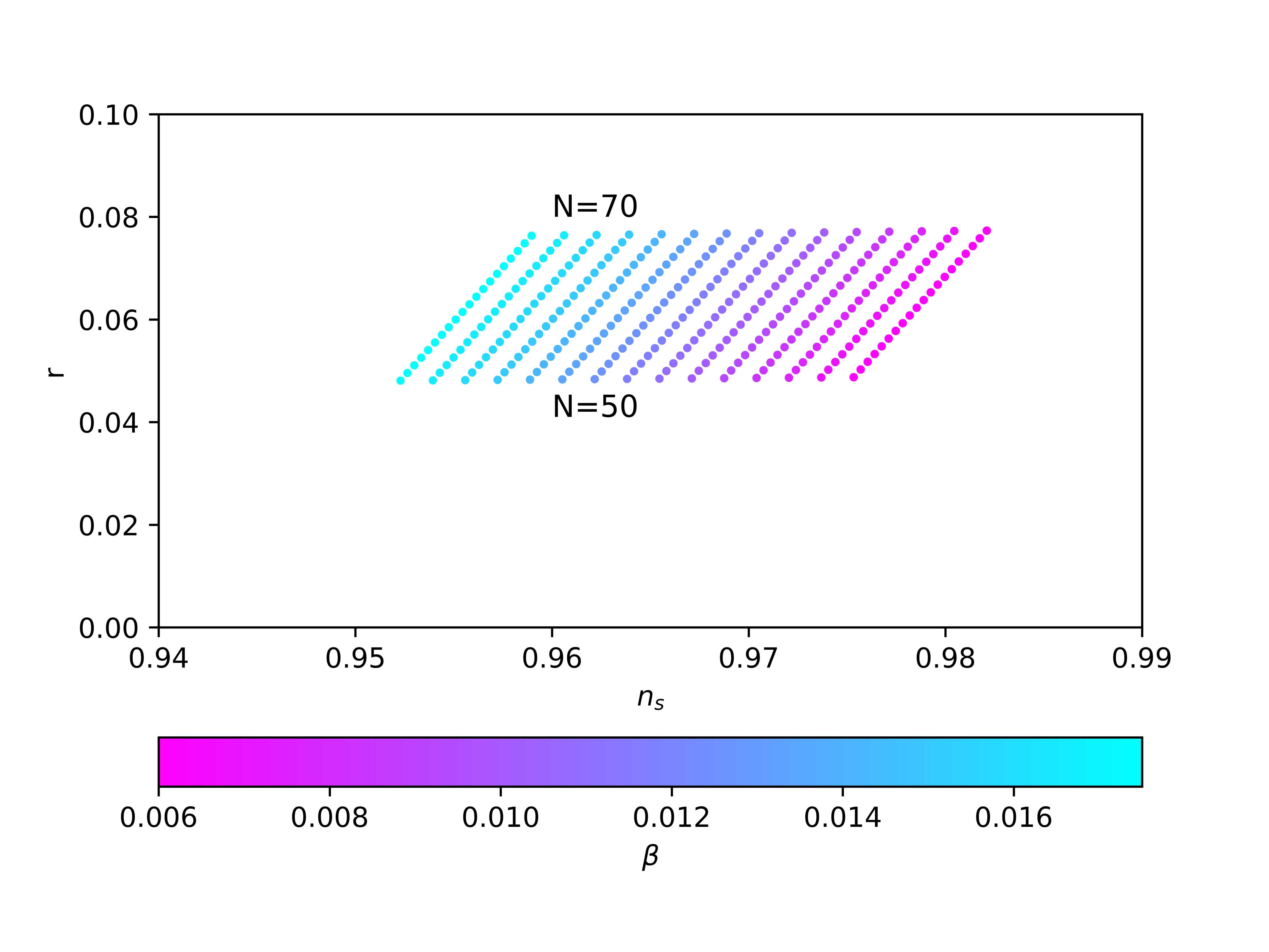
Figure 7: $\gamma=5.5\times 10^{5}$

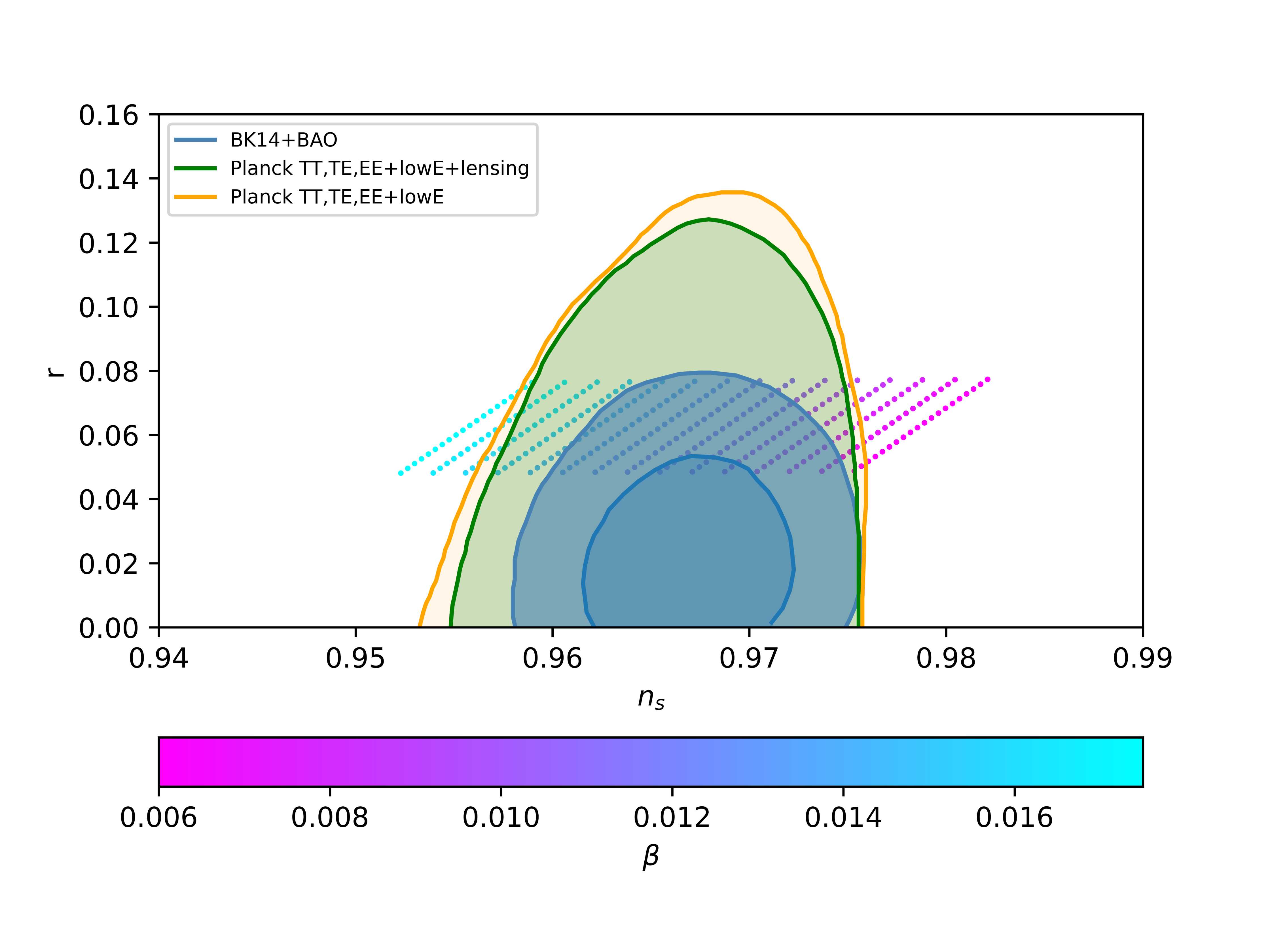
Figure 8: $\gamma=5.5\times 10^{5}$

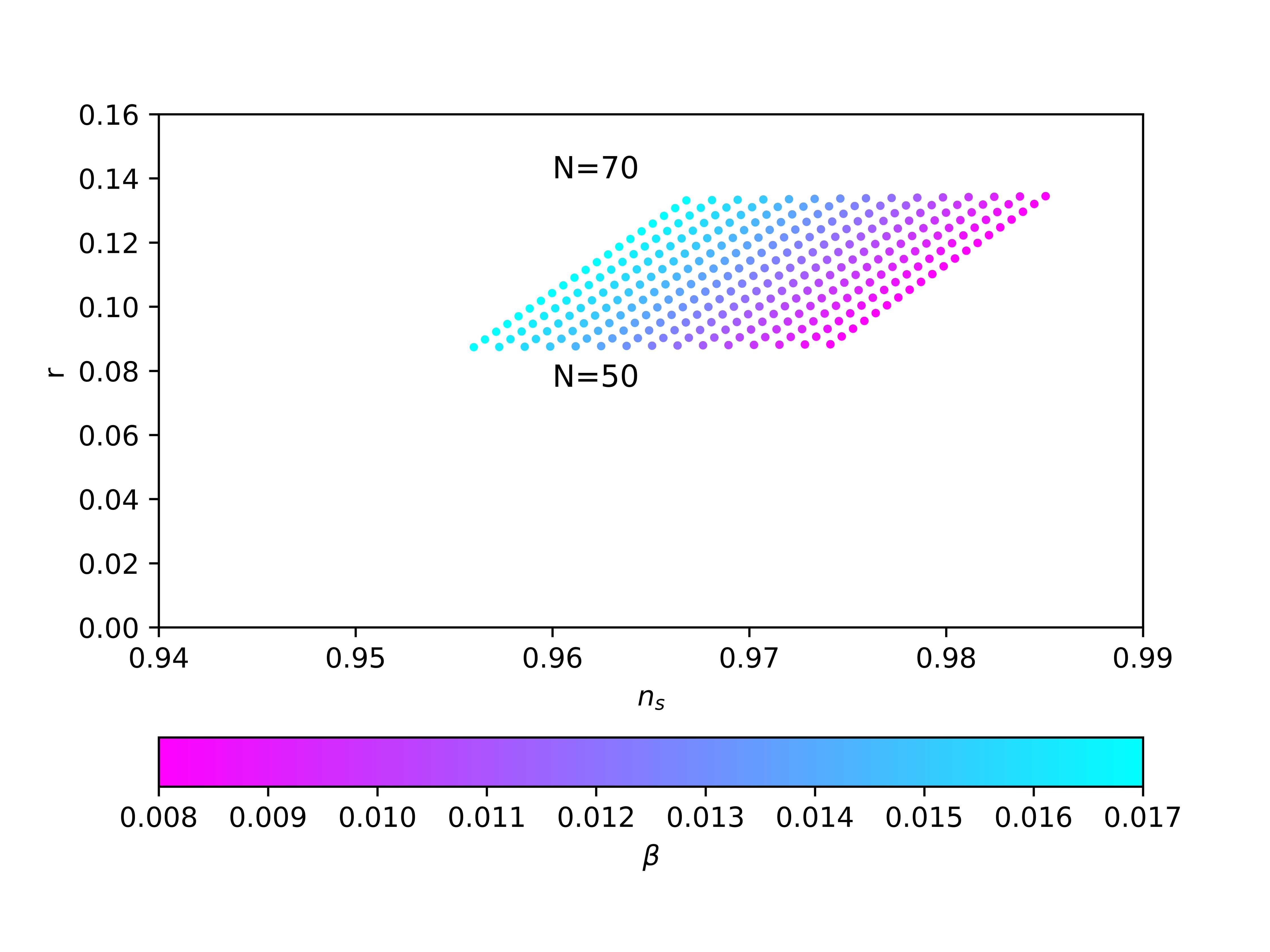
Figure 9: $\gamma=7\times 10^{5}$

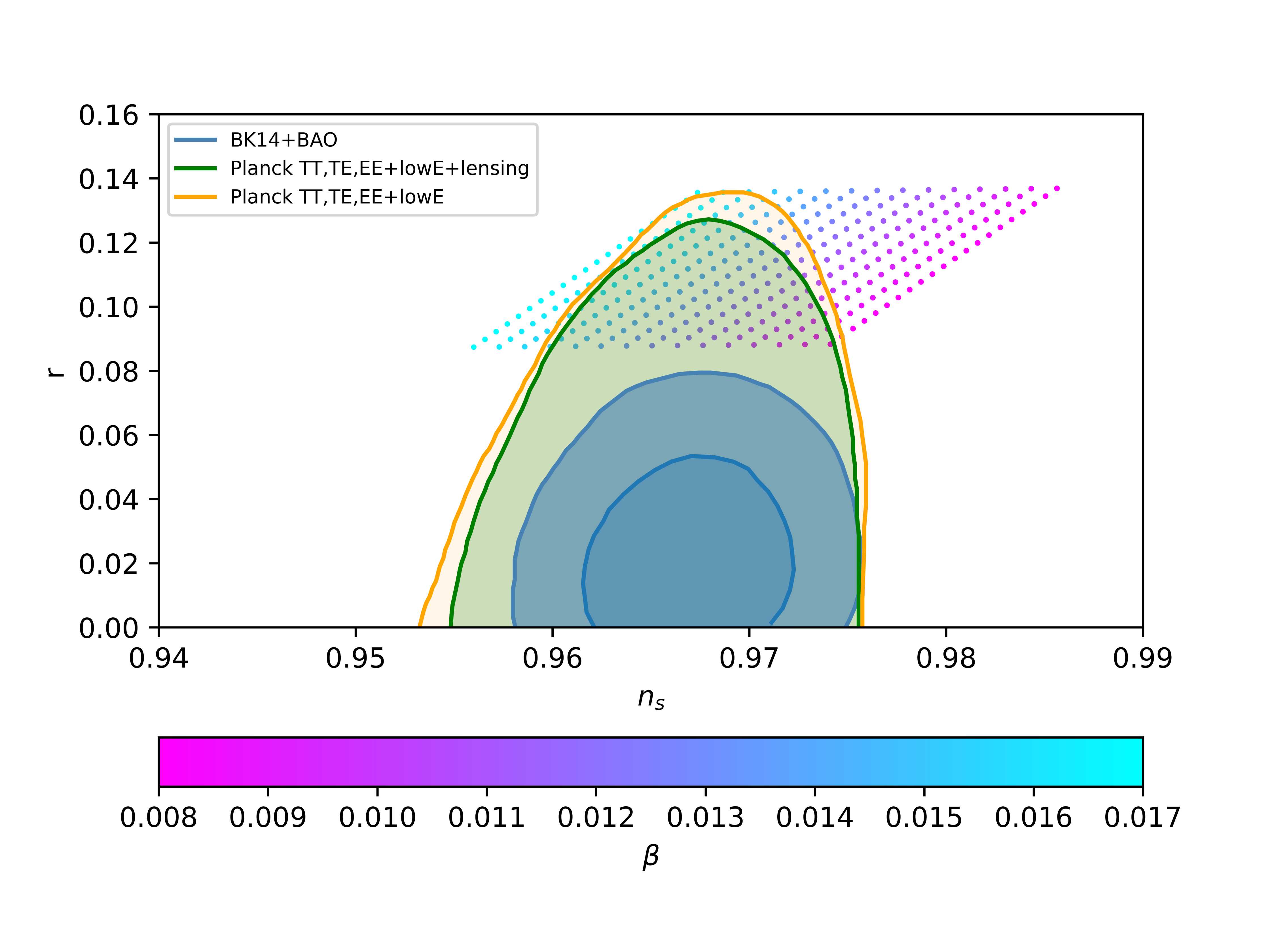
Figure 10: $\gamma=7\times 10^{5}$

IV.    Conclusion

In this paper, we have investigated the possibility of constant-roll in the modified gravity theory using Palatini formalism with action containing non-minimal coupling of $R$ and $R^{2}$ with a scalar field. This formalism helps us in translating $R^{2}$ coupling term into a higher-order kinetic term with a new potential making it an equivalent scalar-tensor theory in the Einstein frame. Then we proceeded to find the equation of motion for the scalar field within this frame and using the constant roll condition, we were able to solve the field equation and find the slow roll parameters. Then we defined our potential for the theory and worked out the expressions for tensor-to-scalar ratio and spectral index. Within the parameter regime of our theory, our results are in complete agreement with the Planck 2018 data and the results with the inclusion of comparison with Planck data are shown in the Figs.($1-10$), thus making constant roll a viable scenario for further research in this model. Most agreed values of $n_{s}$ and $r$ are obtained in the first case. In future, we plan to study the possibility of reheating [87] and the production of primordial black hole [88] within the Palatini formalism for this model.

V.    Acknowledgement

This work is partially supported by DST (Govt. of India) Grant No. SERB/PHY/2021057 and the author RT would like to thank Abhijith Ajith for his help in making plots.

References

- [1] Alan H. Guth “The Inflationary Universe: A Possible Solution to the Horizon and Flatness Problems” In Phys. Rev. D 23, 1981, pp. 347–356 DOI: 10.1103/PhysRevD.23.347
- [2] A.A. Starobinsky “A new type of isotropic cosmological models without singularity” In Physics Letters B 91.1, 1980, pp. 99–102 DOI: https://doi.org/10.1016/0370-2693(80)90670-X
- [3] Andrei D. Linde “A New Inflationary Universe Scenario: A Possible Solution of the Horizon, Flatness, Homogeneity, Isotropy and Primordial Monopole Problems” In Phys. Lett. B 108, 1982, pp. 389–393 DOI: 10.1016/0370-2693(82)91219-9
- [4] A.D. Linde “Chaotic inflation” In Physics Letters B 129.3, 1983, pp. 177–181 DOI: https://doi.org/10.1016/0370-2693(83)90837-7
- [5] David H. Lyth and Antonio Riotto “Particle physics models of inflation and the cosmological density perturbation” In Phys. Rept. 314, 1999, pp. 1–146 DOI: 10.1016/S0370-1573(98)00128-8
- [6] Antonio Riotto “Inflation and the theory of cosmological perturbations” In Astroparticle physics and cosmology. Proceedings: Summer School, Trieste, Italy, Jun 17-Jul 5 2002 14, 2003, pp. 317–413 arXiv:hep-ph/0210162 [hep-ph]
- [7] Daniel Baumann “Inflation” In Physics of the large and the small, TASI 09, proceedings of the Theoretical Advanced Study Institute in Elementary Particle Physics, Boulder, Colorado, USA, 1-26 June 2009, 2011, pp. 523–686 DOI: 10.1142/9789814327183˙0010
- [8] Viatcheslav F. Mukhanov and G.. Chibisov “Quantum Fluctuations and a Nonsingular Universe” In JETP Lett. 33, 1981, pp. 532–535
- [9] Viatcheslav F. Mukhanov and G.. Chibisov “The Vacuum energy and large scale structure of the universe” In Sov. Phys. JETP 56, 1982, pp. 258–265
- [10] Alexei A. Starobinsky “Dynamics of Phase Transition in the New Inflationary Universe Scenario and Generation of Perturbations” In Phys. Lett. B 117, 1982, pp. 175–178 DOI: 10.1016/0370-2693(82)90541-X
- [11] Alan H. Guth and So-Young Pi “Fluctuations in the New Inflationary Universe” In Phys. Rev. Lett. 49 American Physical Society, 1982, pp. 1110–1113 DOI: 10.1103/PhysRevLett.49.1110
- [12] Robert H. Brandenberger “INFLATIONARY UNIVERSE MODELS AND THE FORMATION OF STRUCTURE” In 8th Santa Cruz Summer Workshop in Astronomy and Astrophysics: Nearly Normal Galaxies from the Planch Time to the Present, 1986
- [13] James M. Bardeen, Paul J. Steinhardt and Michael S. Turner “Spontaneous creation of almost scale-free density perturbations in an inflationary universe” In Phys. Rev. D 28 American Physical Society, 1983, pp. 679–693 DOI: 10.1103/PhysRevD.28.679
- [14] C.. Bennett “First year Wilkinson Microwave Anisotropy Probe (WMAP) observations: Preliminary maps and basic results” In Astrophys. J. Suppl. 148, 2003, pp. 1–27 DOI: 10.1086/377253
- [15] D.. Spergel “Wilkinson Microwave Anisotropy Probe (WMAP) three year results: implications for cosmology” In Astrophys. J. Suppl. 170, 2007, pp. 377 DOI: 10.1086/513700
- [16] N. Aghanim “Planck 2018 results. VI. Cosmological parameters” [Erratum: Astron.Astrophys. 652, C4 (2021)] In Astron. Astrophys. 641, 2020, pp. A6 DOI: 10.1051/0004-6361/201833910
- [17] M. Novello and S.. Bergliaffa “Bouncing Cosmologies” In Phys. Rept. 463, 2008, pp. 127–213 DOI: 10.1016/j.physrep.2008.04.006
- [18] S. Nojiri, S.. Odintsov and V.. Oikonomou “Modified Gravity Theories on a Nutshell: Inflation, Bounce and Late-time Evolution” In Phys. Rept. 692, 2017, pp. 1–104 DOI: 10.1016/j.physrep.2017.06.001
- [19] Yi-Fu Cai, Robert Brandenberger and Patrick Peter “Anisotropy in a non-singular bounce” In Classical and Quantum Gravity 30.7 IOP Publishing, 2013, pp. 075019 DOI: 10.1088/0264-9381/30/7/075019
- [20] David Wands “Duality invariance of cosmological perturbation spectra” In Physical Review D 60.2 American Physical Society (APS), 1999 DOI: 10.1103/physrevd.60.023507
- [21] Fabio Finelli and Robert Brandenberger “On the generation of a scale invariant spectrum of adiabatic fluctuations in cosmological models with a contracting phase” In Phys. Rev. D 65, 2002, pp. 103522 DOI: 10.1103/PhysRevD.65.103522
- [22] Robert H. Brandenberger “Alternatives to the inflationary paradigm of structure formation” In Int. J. Mod. Phys. Conf. Ser. 01, 2011, pp. 67–79 DOI: 10.1142/S2010194511000109
- [23] Robert H. Brandenberger “The Matter Bounce Alternative to Inflationary Cosmology”, 2012 arXiv:1206.4196 [astro-ph.CO]
- [24] Bao-Fei Li, Sahil Saini and Parampreet Singh “Primordial power spectrum from a matter-Ekpyrotic bounce scenario in loop quantum cosmology” In Phys. Rev. D 103.6, 2021, pp. 066020 DOI: 10.1103/PhysRevD.103.066020
- [25] Asha B. Modan, Sukanta Panda and Arun Rana “Imprints of anisotropy on the power spectrum in matter dominated bouncing universe as background” In Eur. Phys. J. C 82.10, 2022, pp. 887 DOI: 10.1140/epjc/s10052-022-10867-z
- [26] Alexei A. Starobinsky “A New Type of Isotropic Cosmological Models Without Singularity” In Phys. Lett. B 91, 1980, pp. 99–102 DOI: 10.1016/0370-2693(80)90670-X
- [27] Antonio De Felice and Shinji Tsujikawa “f(R) theories” In Living Rev. Rel. 13, 2010, pp. 3 DOI: 10.12942/lrr-2010-3
- [28] Thomas P. Sotiriou and Valerio Faraoni “f(R) Theories Of Gravity” In Rev. Mod. Phys. 82, 2010, pp. 451–497 DOI: 10.1103/RevModPhys.82.451
- [29] Salvatore Capozziello and Mariafelicia De Laurentis “Extended Theories of Gravity” In Phys. Rept. 509, 2011, pp. 167–321 DOI: 10.1016/j.physrep.2011.09.003
- [30] Timothy Clifton, Pedro G. Ferreira, Antonio Padilla and Constantinos Skordis “Modified Gravity and Cosmology” In Phys. Rept. 513, 2012, pp. 1–189 DOI: 10.1016/j.physrep.2012.01.001
- [31] S.. Odintsov and V.. Oikonomou “Inflationary -attractors from gravity” In Phys. Rev. D 94.12, 2016, pp. 124026 DOI: 10.1103/PhysRevD.94.124026
- [32] Thomas P. Sotiriou “f(R) gravity and scalar-tensor theory” In Class. Quant. Grav. 23, 2006, pp. 5117–5128 DOI: 10.1088/0264-9381/23/17/003
- [33] Thomas P. Sotiriou and Stefano Liberati “Metric-affine f(R) theories of gravity” In Annals Phys. 322, 2007, pp. 935–966 DOI: 10.1016/j.aop.2006.06.002
- [34] Monica Borunda, Bert Janssen and Mar Bastero-Gil “Palatini versus metric formulation in higher curvature gravity” In JCAP 11, 2008, pp. 008 DOI: 10.1088/1475-7516/2008/11/008
- [35] Gonzalo J. Olmo “Palatini Approach to Modified Gravity: f(R) Theories and Beyond” In Int. J. Mod. Phys. D 20, 2011, pp. 413–462 DOI: 10.1142/S0218271811018925
- [36] Florian Bauer and Durmus A. Demir “Inflation with Non-Minimal Coupling: Metric versus Palatini Formulations” In Phys. Lett. B 665, 2008, pp. 222–226 DOI: 10.1016/j.physletb.2008.06.014
- [37] Nicola Tamanini and Carlo R. Contaldi “Inflationary Perturbations in Palatini Generalised Gravity” In Phys. Rev. D 83, 2011, pp. 044018 DOI: 10.1103/PhysRevD.83.044018
- [38] Amy Lloyd-Stubbs and John McDonald “Sub-Planckian Inflation in the Palatini Formulation of Gravity with an term”, 2020 arXiv:2002.08324 [hep-ph]
- [39] Paulo M. Sá “Unified description of dark energy and dark matter within the generalized hybrid metric-Palatini theory of gravity”, 2020 arXiv:2002.09446 [gr-qc]
- [40] Ignatios Antoniadis, Angelos Lykkas and Kyriakos Tamvakis “Constant-roll in the Palatini- models” In JCAP 04.04, 2020, pp. 033 DOI: 10.1088/1475-7516/2020/04/033
- [41] D.M. Ghilencea “Palatini quadratic gravity: spontaneous breaking of gauged scale symmetry and inflation”, 2020 arXiv:2003.08516 [hep-th]
- [42] Konstantinos Dimopoulos, Alexandros Karam, Samuel Sánchez López and Eemeli Tomberg “Palatini R 2 quintessential inflation” In JCAP 10, 2022, pp. 076 DOI: 10.1088/1475-7516/2022/10/076
- [43] Claire Rigouzzo and Sebastian Zell “Coupling metric-affine gravity to a Higgs-like scalar field” In Phys. Rev. D 106.2, 2022, pp. 024015 DOI: 10.1103/PhysRevD.106.024015
- [44] Christian Dioguardi, Antonio Racioppi and Eemeli Tomberg “Slow-roll inflation in Palatini F(R) gravity” In JHEP 06, 2022, pp. 106 DOI: 10.1007/JHEP06(2022)106
- [45] Dhong Yeon Cheong, Sung Mook Lee and Seong Chan Park “Reheating in models with non-minimal coupling in metric and Palatini formalisms” In JCAP 02.02, 2022, pp. 029 DOI: 10.1088/1475-7516/2022/02/029
- [46] Angelos Lykkas and Kyriakos Tamvakis “Extended interactions in the Palatini- inflation” In JCAP 08.043, 2021 DOI: 10.1088/1475-7516/2021/08/043
- [47] Ioannis D. Gialamas, Alexandros Karam, Angelos Lykkas and Thomas D. Pappas “Palatini-Higgs inflation with nonminimal derivative coupling” In Phys. Rev. D 102.6, 2020, pp. 063522 DOI: 10.1103/PhysRevD.102.063522
- [48] Javier Rubio and Eemeli S. Tomberg “Preheating in Palatini Higgs inflation” In JCAP 04, 2019, pp. 021 DOI: 10.1088/1475-7516/2019/04/021
- [49] Syksy Rasanen “Higgs inflation in the Palatini formulation with kinetic terms for the metric”, 2018 DOI: 10.21105/astro.1811.09514
- [50] Antonio Racioppi “New universal attractor in nonminimally coupled gravity: Linear inflation” In Phys. Rev. D 97.12, 2018, pp. 123514 DOI: 10.1103/PhysRevD.97.123514
- [51] Flavio Bombacigno and Giovanni Montani “Big bounce cosmology for Palatini gravity with a Nieh–Yan term” In Eur. Phys. J. C 79.5, 2019, pp. 405 DOI: 10.1140/epjc/s10052-019-6918-x
- [52] I. Antoniadis, A. Karam, A. Lykkas and K. Tamvakis “Palatini inflation in models with an term” In JCAP 11, 2018, pp. 028 DOI: 10.1088/1475-7516/2018/11/028
- [53] I. Antoniadis et al. “Rescuing Quartic and Natural Inflation in the Palatini Formalism” In JCAP 03, 2019, pp. 005 DOI: 10.1088/1475-7516/2019/03/005
- [54] Kristjan Kannike, Aleksei Kubarski, Luca Marzola and Antonio Racioppi “A minimal model of inflation and dark radiation” In Phys. Lett. B 792, 2019, pp. 74–80 DOI: 10.1016/j.physletb.2019.03.025
- [55] Juan P. Almeida, Nicolás Bernal, Javier Rubio and Tommi Tenkanen “Hidden Inflaton Dark Matter” In JCAP 03, 2019, pp. 012 DOI: 10.1088/1475-7516/2019/03/012
- [56] Tommi Tenkanen “Minimal Higgs inflation with an term in Palatini gravity” In Phys. Rev. D 99.6, 2019, pp. 063528 DOI: 10.1103/PhysRevD.99.063528
- [57] Kari Enqvist, Tomi Koivisto and Gerasimos Rigopoulos “Non-metric chaotic inflation” In JCAP 05, 2012, pp. 023 DOI: 10.1088/1475-7516/2012/05/023
- [58] Andrzej Borowiec, Michal Kamionka, Aleksandra Kurek and Marek Szydlowski “Cosmic acceleration from modified gravity with Palatini formalism” In JCAP 02, 2012, pp. 027 DOI: 10.1088/1475-7516/2012/02/027
- [59] Massimo Giovannini “Post-inflationary phases stiffer than radiation and Palatini formulation” In Class. Quant. Grav. 36.23, 2019, pp. 235017 DOI: 10.1088/1361-6382/ab52a8
- [60] Aleksander Stachowski, Marek Szydłowski and Andrzej Borowiec “Starobinsky cosmological model in Palatini formalism” In Eur. Phys. J. C 77.6, 2017, pp. 406 DOI: 10.1140/epjc/s10052-017-4981-8
- [61] Chengjie Fu, Puxun Wu and Hongwei Yu “Inflationary dynamics and preheating of the nonminimally coupled inflaton field in the metric and Palatini formalisms” In Phys. Rev. D 96.10, 2017, pp. 103542 DOI: 10.1103/PhysRevD.96.103542
- [62] Syksy Rasanen and Pyry Wahlman “Higgs inflation with loop corrections in the Palatini formulation” In JCAP 11, 2017, pp. 047 DOI: 10.1088/1475-7516/2017/11/047
- [63] Antonio Racioppi “Coleman-Weinberg linear inflation: metric vs. Palatini formulation” In JCAP 12, 2017, pp. 041 DOI: 10.1088/1475-7516/2017/12/041
- [64] Tommi Markkanen, Tommi Tenkanen, Ville Vaskonen and Hardi Veermäe “Quantum corrections to quartic inflation with a non-minimal coupling: metric vs. Palatini” In JCAP 03, 2018, pp. 029 DOI: 10.1088/1475-7516/2018/03/029
- [65] Laur Järv, Antonio Racioppi and Tommi Tenkanen “Palatini side of inflationary attractors” In Phys. Rev. D 97.8, 2018, pp. 083513 DOI: 10.1103/PhysRevD.97.083513
- [66] Nilay Bostan “Quadratic, Higgs and hilltop potentials in the Palatini gravity”, 2019 arXiv:1908.09674 [astro-ph.CO]
- [67] Ioannis D. Gialamas and A.B. Lahanas “Reheating in Palatini inflationary models” In Phys. Rev. D 101.8, 2020, pp. 084007 DOI: 10.1103/PhysRevD.101.084007
- [68] Mikhail Shaposhnikov, Andrey Shkerin and Sebastian Zell “Quantum Effects in Palatini Higgs Inflation”, 2020 arXiv:2002.07105 [hep-ph]
- [69] Florian Bauer and Durmus A. Demir “Higgs-Palatini Inflation and Unitarity” In Phys. Lett. B 698, 2011, pp. 425–429 DOI: 10.1016/j.physletb.2011.03.042
- [70] Aleksander Kozak and Andrzej Borowiec “Palatini frames in scalar–tensor theories of gravity” In Eur. Phys. J. C 79.4, 2019, pp. 335 DOI: 10.1140/epjc/s10052-019-6836-y
- [71] Ryusuke Jinno, Kunio Kaneta, Kin-ya Oda and Seong Chan Park “Hillclimbing inflation in metric and Palatini formulations” In Phys. Lett. B 791, 2019, pp. 396–402 DOI: 10.1016/j.physletb.2019.03.012
- [72] Tommi Tenkanen “Tracing the high energy theory of gravity: an introduction to Palatini inflation” In Gen. Rel. Grav. 52.4, 2020, pp. 33 DOI: 10.1007/s10714-020-02682-2
- [73] Hyerim Noh and Jai-chqn Hwang “Inflationary spectra in generalized gravity: Unified forms” In Phys. Lett. B 515, 2001, pp. 231–237 DOI: 10.1016/S0370-2693(01)00875-9
- [74] N.. Tsamis and Richard P. Woodard “Improved estimates of cosmological perturbations” In Phys. Rev. D 69, 2004, pp. 084005 DOI: 10.1103/PhysRevD.69.084005
- [75] Konstantinos Dimopoulos “Ultra slow-roll inflation demystified” In Phys. Lett. B 775, 2017, pp. 262–265 DOI: 10.1016/j.physletb.2017.10.066
- [76] Chris Pattison, Vincent Vennin, Hooshyar Assadullahi and David Wands “The attractive behaviour of ultra-slow-roll inflation” In JCAP 08, 2018, pp. 048 DOI: 10.1088/1475-7516/2018/08/048
- [77] Zhu Yi and Yungui Gong “On the constant-roll inflation” In JCAP 03, 2018, pp. 052 DOI: 10.1088/1475-7516/2018/03/052
- [78] Lilia Anguelova, Peter Suranyi and L.. Wijewardhana “Systematics of Constant Roll Inflation” In JCAP 02, 2018, pp. 004 DOI: 10.1088/1475-7516/2018/02/004
- [79] Francesco Cicciarella, Joel Mabillard and Mauro Pieroni “New perspectives on constant-roll inflation” In JCAP 01, 2018, pp. 024 DOI: 10.1088/1475-7516/2018/01/024
- [80] Merce Guerrero, Diego Rubiera-Garcia and Diego Saez-Chillon Gomez “Constant roll inflation in multifield models” In Phys. Rev. D 102, 2020, pp. 123528 DOI: 10.1103/PhysRevD.102.123528
- [81] Mohammad Hossein Namjoo, Hassan Firouzjahi and Misao Sasaki “Violation of non-Gaussianity consistency relation in a single field inflationary model” In EPL 101.3, 2013, pp. 39001 DOI: 10.1209/0295-5075/101/39001
- [82] Nayan Das and Sukanta Panda “Inflation and Reheating in f(R,h) theory formulated in the Palatini formalism” In JCAP 05, 2021, pp. 019 DOI: 10.1088/1475-7516/2021/05/019
- [83] Tonguc Rador “f(R) Gravities a la Brans-Dicke” In Phys. Lett. B 652, 2007, pp. 228–232 DOI: 10.1016/j.physletb.2007.07.034
- [84] S.. Odintsov and V.. Oikonomou “Constant-roll -Inflation Dynamics” In Class. Quant. Grav. 37.2, 2020, pp. 025003 DOI: 10.1088/1361-6382/ab5c9d
- [85] Jai-chan Hwang and Hyerim Noh “Cosmological perturbations in a generalized gravity including tachyonic condensation” In Phys. Rev. D 66, 2002, pp. 084009 DOI: 10.1103/PhysRevD.66.084009
- [86] Jai-chan Hwang and Hyerim Noh “Classical evolution and quantum generation in generalized gravity theories including string corrections and tachyon: Unified analyses” In Phys. Rev. D 71, 2005, pp. 063536 DOI: 10.1103/PhysRevD.71.063536
- [87] V.. Oikonomou “Reheating in Constant-roll Gravity” In Mod. Phys. Lett. A 32.33, 2017, pp. 1750172 DOI: 10.1142/S0217732317501723
- [88] Hayato Motohashi, Shinji Mukohyama and Michele Oliosi “Constant Roll and Primordial Black Holes” In JCAP 03, 2020, pp. 002 DOI: 10.1088/1475-7516/2020/03/002