Beyond Incompatibility: Trade-offs between Mutually Exclusive Fairness Criteria in Machine Learning and Law

Abstract.

Trustworthy AI is becoming ever more important in both machine learning and legal domains. One important consequence is that decision makers must seek to guarantee a ‘fair’, i.e., non-discriminatory, algorithmic decision procedure. However, there are several competing notions of algorithmic fairness that have been shown to be mutually incompatible under realistic factual assumptions. This concerns, for example, the widely used fairness measures of ‘calibration within groups’ and ‘balance for the positive/negative class’. In this paper, we present a novel algorithm (FAir Interpolation Method: FAIM) for continuously interpolating between these three fairness criteria. Thus, an initially unfair prediction can be remedied to, at least partially, meet a desired, weighted combination of the respective fairness conditions. We demonstrate the effectiveness of our algorithm when applied to synthetic data, the COMPAS data set, and a new, real-world data set from the e-commerce sector. Finally, we discuss to what extent FAIM can be harnessed to comply with conflicting legal obligations. The analysis suggests that it may operationalize duties in traditional legal fields, such as credit scoring and criminal justice proceedings, but also for the latest AI regulations put forth in the EU, like the recently enacted Digital Markets Act.

1. Introduction

As machine learning (ML) progressively permeates all sectors of society, responsible and trustworthy AI development is more crucial than ever ((Dignum, 2019; Grodzinsky et al., 2011; Thiebes et al., 2021)). Increasingly, this debate spills over from the ethics and machine learning communities to the legal domain ((Laux et al., 2022)), where different regulatory frameworks for ensuring trustworthy AI are emerging. In this context, discrimination against protected groups in decisions facilitated by ML models remains a key challenge ((Wachter, 2022)). Non-discrimination legislation applying to biased AI systems does exist in the US and the EU, but loopholes and enforcement problems remain ((Barocas and Selbst, 2016; Hacker, 2018; Zuiderveen Borgesius, 2020; Wachter et al., 2021b; Wachter, 2022)). Hence, the AI Act, proposed by the EU Commission in 2021 and set to be enacted soon in the EU, adds further duties for ML developers such as the duty to evaluate of training data for potential biases (Article 10(2) AI Act), the duty to use representative training data (Article 10(3) AI Act) and the duty to prevent biased feedback loops (Article 15(3) AI Act) ((Veale and Borgesius, 2021; Ebers et al., 2021; Hacker, 2021)). This is backed up by a framework for AI liability proposed in September 2022 by the EU Commission ((Hacker, 2022a)). Moreover, the recently enacted EU Digital Markets Act (DMA) now compels large online platforms to engage in ‘fair and non-discriminatory’ ranking (Article 6(5) DMA).

The laudable idea behind such approaches is to force developers to consider, and potentially eliminate, biases during the design of ML models. Such non-discriminatory models are called ‘fair’ in the ML community ((Mitchell et al., 2021; Dwork et al., 2012)). However, foundational papers at the intersection of machine learning and the law have shown that, under realistic assumptions, several desirable fairness criteria are mutually incompatibility ((Kleinberg et al., 2016)). This poses a significant challenge as the law, in general, prohibits discrimination without explicitly favoring one metric over another. Rather, a core tenet of legal research and jurisprudence is that conflicting rights or interests need to be balanced, i.e., be partially realized to satisfy each of the mutually incompatible demands to the extent that conditions warrant ((De Vries, 2013; Morijn, 2006)). Lawmakers, courts and regulators therefore need fairness frameworks that move beyond the mere statement of incompatibility. Simultaneously, ML research may benefit from the legal tradition of balancing by inducing decision makers and developers to refine algorithms implementing a balance between the normative trade-offs inherent in the mutually incompatible fairness criteria ((Hertweck and Räz, 2022)). Our paper develops one such algorithm allowing decision makers to interpolate between three different incompatible fairness criteria singled out for their importance in previous research. These three fairness criteria are described below.

There are various ways in which unfairness, i.e., discrimination against certain groups  ((Friedman and Nissenbaum, 1996)), may enter an ML model ((Calders and Žliobaitė, 2013)). For example, the model may perpetuate historical biases present in the training data; use non-representative training data; or optimize for a target variable which unwittingly encodes differential access of individuals or groups ((Barocas and Selbst, 2016)). The result of such biased modeling may be that false positive or false negative rates differ between groups of individuals. Specific fairness metrics such as equalized odds, quantifying the difference of false positive and false negative rates between groups  ((Hardt et al., 2016)), are used to quantify how much a classifier systematically rewards or punishes one group more than another with respect to ground truth. Even if a classifier is fair in terms of equalized odds, its prediction scores can lead to unfair outcomes if they are uncalibrated, as decision makers are not able to reliably interpret its output ((Zadrozny and Elkan, 2001; Jiang et al., 2012)). What is worse, if a classifier emits scores that are differently calibrated between groups, identical scores have different meanings for different protected groups, again leading to unfair outcomes ((Kleinberg et al., 2016)).

Given that equality of false positive rates between groups, equality of false negative rates between groups, and calibration between groups are all important fairness criteria ((Corbett-Davies and Goel, 2018)), it would be ideal if a classifier could satisfy all three. Unfortunately, previous work shows that simultaneously fulfilling all three of these fairness criteria is impossible, except under highly constrained circumstances such as when a classifier achieves 100% accuracy with each instance receiving a prediction score of exactly 0 or 1 ((Chouldechova, 2017; Kleinberg et al., 2016; Pleiss et al., 2017)). Pleiss et al. (2017) attempt to find a relaxed notion of error rate difference that can be simultaneously achieved alongside group calibration. However, they demonstrate that one may only simultaneously achieve group calibration with a relaxed version of one of either equalized false positive or false negative rates. Furthermore, they show that classifiers simultaneously satisfying two of these three fairness criteria must engage in the equivalent of randomizing a certain percentage of predictions. Thus, the authors suggest that practitioners should only attempt to satisfy one of the three fairness criteria based on importance, instead of trying to simultaneously fulfill a relaxed notion of two of them. Often, however, all three fairness notions embody valid concerns of different groups ((Corbett-Davies and Goel, 2018)). Merely satisfying one of them may not do justice to the various interests and rights of the groups, and, as discussed above, might even amount to unjustified discrimination if the law demands a balance rather than an absolute priority of one criterion.

Building on the assumption that a decision makers should determine, within the constraints of the law, which combination of the three fairness criteria is most crucial towards a fair result in practice, our work introduces a new post-processing algorithm called FAir Interpolation Method (FAIM). It allows decision makers to consciously and continuously interpolate between fairness criteria. The algorithm is based on the notion that, given a classifier, a representative evaluation data set, and the corresponding prediction scores for each group, any one of the three fairness criteria could be satisfied by applying a certain fairness criteria specific score mapping function mapping scores from the distribution outputted by the model to a fair score distribution. Given three such fairness criteria specific score distributions, FAIM uses optimal transport to continuously interpolate between them. This leads to a mapping function that can be applied to new classifier predictions, post hoc, to achieve a desired, weighted combination of the respective fairness criteria. FAIM cannot be used to fully satisfy all three fairness criteria simultaneously, but it does give the practitioner a powerful tool to make a continuous compromise along the fairness criteria simplex, and thus to account for different concerns each fairness criterion encompasses.

The remainder of the article is organized as follows. First, related work is outlined in detail. Next, the mathematical foundations regarding fairness criteria incompatibility and optimal transport are addressed. Based on this, FAIM is introduced, and tested empirically in three experiments. In the first experiment, FAIM is applied to a synthetic classifier that produces two distinct score distributions for two respective groups. Here the properties of FAIM are elucidated under controlled conditions. In the second experiment, FAIM is tested on the COMPAS data set, on which the COMPAS algorithm famously scores individuals for recidivism risk. In the last experiment, FAIM is applied to product rankings from the European e-commerce platform Zalando. Here, we evaluate our model in terms of typical fairness problems arising in e-commerce rankings. The discussion takes up the results of the experiments and adds a specific legal perspective. We show how FAIM may be harnessed to trade off conflicting legal requirements across a wide variety of domains: credit scoring, criminal justice decisions, and fair rankings according to the DMA.

Overall, the paper brings together technical and legal perspectives on fairness criteria to take both discourses beyond incompatibility statements. In this way, decision makers may flexibly adapt ML models to different use cases in which varying interests of protected groups may necessitate different trade-offs between the involved fairness criteria. Simultaneously, gradually balancing the different fairness criteria, rather than prioritizing only one of them, will often be conducive to fulfilling legal requirements, both in established legal domains and in novel regulatory frameworks, such as the DMA.

2. Related Work

The incompatibility of various different fairness criteria in algorithmic decision making has been the subject of intense research in recent years.  Friedler et al. (2016) discuss the contrast between individual and group fairness. While these results hint at an incompatibility between individual and group fairness and relate these notions to two opposing worldviews, there is no rigorous proof of such incompatibility, and no discussion of possible intermediate worldviews. Some of the results in  Feldman et al. (2015) and  Zehlike et al. (2020) can be viewed as proposals on how to continuously navigate between the two extremes.

The recidivism prediction problem was treated in  Kleinberg et al. (2016); Chouldechova (2017), with the result that a prediction algorithm must necessarily be unfair with regard to certain fairness criteria under realistic factual assumptions. In particular, Kleinberg et al. (2016) show the mutual incompatibility between calibration within groups and balance for the positive/negative classes in the (typical) case of unequal base rates. These fairness criteria also underlie the present contribution. The framework of Kleinberg et al. (2016) is thoroughly reviewed below; let us remark here only that the mentioned criteria of  Kleinberg et al. (2016) acknowledge and accept the possibility of empirically observed disparities between different groups, but require the equal treatment of individuals in different groups conditional on their similarity according to ‘ground truth’. The competing criterion of calibration within groups concerns the accuracy of the algorithm and is shown to conflict with the other two criteria.

The use of optimal transport methods in algorithmic fairness has become increasingly popular  ((Dwork et al., 2012; Feldman et al., 2015; Gordaliza et al., 2019; Zehlike et al., 2020; Chiappa et al., 2020; Chiappa and Pacchiano, 2021)), applying optimal transport to trade-offs between individual vs group fairness, and accuracy vs fairness. Optimal transport is a mathematical tool that provides a very natural notion of distance of two probability distributions (the Wasserstein or earth mover distance) and, moreover, gives an optimal (in a specific sense) way to translate between these distributions by means of an optimal transport map or at least an optimal transport plan, the latter requiring some form of randomization. In (Zehlike et al., 2020), particularly, an important role is played by the Wasserstein-2 barycenter of several probability distributions and the displacement interpolation that allows to continuously interpolate between various distributions. We make use of these techniques in the present article.

The literature at the intersection of law and computer science has, in the past few years, increasingly discussed how legal non-discrimination requirements can be integrated into code, and vice versa  ((Zehlike et al., 2020; Hacker, 2018; Wachter et al., 2021a, b; Zuiderveen Borgesius, 2020; Gerards and Borgesius, 2022; Wachter, 2020, 2022; Barocas and Selbst, 2016; Raghavan et al., 2020; Hellman, 2020; Nachbar, 2020)). This strand of research has focused particularly on remedying discrimination in criminal justice proceedings ((Berk et al., 2021; Starr, 2014; Mayson, 2019; Selbst, 2017; Katyal, 2019; Eaglin, 2017; Huq, 2019; Pruss, 2021)) and in other high-stakes AI decisions ((Veale et al., 2018)), such as employment contexts ((Raghavan et al., 2020)), credit scoring ((Bono et al., 2021)), or university admissions ((Zehlike et al., 2020)). More specifically, (Wachter et al. (2021a)) rightly point out that the reliance on fairness metrics based on ground truth may perpetuate biases if that ground truth itself is skewed against protected groups. This is a concern, for example, in criminal justice settings ((Berk et al., 2021; Bao et al., 2021)). We incorporate this constraint into the application perimeter of our algorithm (see Part 6.3). Conversely, in the e-commerce sector, numerous publications deal with the emerging competition law framework for digital markets, for example the DMA ((Eifert et al., 2021; Hacker, 2022b; Brouwer, 2021; Cabral et al., 2021; Laux et al., 2021; Podszun and Bongartz, 2021)). However, they do not, to our knowledge, specifically develop algorithms to solve legal questions arising in this field.

Existing publications often use US law as the relevant yardstick ((Barocas and Selbst, 2016; Raghavan et al., 2020; Wachter, 2022; Selbst and Barocas, 2022; Hellman, 2020; Gillis and Spiess, 2019; Kim, 2017, 2022)), but have lately increasingly incorporated explicit discussions of EU law as well ((Zehlike et al., 2020; Hacker, 2018; Wachter et al., 2021a, b; Zuiderveen Borgesius, 2020; Gerards and Borgesius, 2022; Wachter, 2020, 2022; Veale and Binns, 2017)). Our paper builds on and expands this strand of research by offering a novel method to trade off and implement competing technical and legal fairness constraints. In three case studies, it demonstrates the potential of FAIM to integrate varying legal dimensions of fairness in ML settings, particularly in the criminal justice and credit scoring domain. The third case study tackles an, to our knowledge, entirely new field of law from an algorithmic fairness perspective: the EU Digital Markets Act (DMA).

3. Mathematical Theory and Algorithmic Implementation

This section introduces FAIM, our interpolation framework that allows a continuous shift between three mutually exclusive fairness notions, as presented in Kleinberg et al. (2016). We first provide a brief summary of the findings from Kleinberg et al. (2016) to make the reader familiar with the three fairness notions and establish necessary terminology. We then briefly present mathematical preliminaries from optimal transport theory. Finally we describe the mathematical theory of our algorithm as well as its implementation in parallel, to help the reader translate between the formulas and the code. We present the method in pseudocode in Algorithm 1.

For the simplicity of presentation, we consider a population of individuals partitioned into two groups, indexed by $t=1,2$. Note first, that individuals need not be human, but could also be products, companies, etc., and second, that our method applies just as well to a setting with more than two groups.

Each individual, regardless of group membership, is either truly ‘positive’ or ‘negative’ with respect to some trait of interest; i.e., in criminal justice, an individual would be ‘positive’ if they were to commit a certain type of crime within a given period in the future, and negative if not. The attributes ‘positive’ and ‘negative’ do not carry any normative meaning and are thus interchangeable, but we will refer to such a classification as ‘ground truth’: It is assumed that the assignments of the positive/negative label reflect reality (we will shortly discuss the limitations of this assumption).

Furthermore, each individual is assigned a score by some algorithm (in the broadest sense). The score, which can take as its value any real number in the interval $[0,1]$, is supposed to reflect the probability that the given individual is positive. Therefore, if the ground truth were fully known to the algorithm, it would assign value 1 to positive individuals and 0 to negative ones. This unlikely scenario is known as perfect prediction.

A note on terminology: When we say that an individual is truly negative/positive, we mean that the individual is negative/positive according to ground truth, regardless of their predicted score. This should not be confused with the common terminology in which a ‘true negative’ is an individual who is negative in ground truth and who, in addition, receives a negative prediction. In our setting, anyway, the predictions are not binary, but in terms of a continuous score between zero and one.

3.1. Incompatibility of Fairness Criteria

The main result from Kleinberg et al. (2016) states that, in the setting described above, three natural fairness criteria are mutually incompatible except under trivial circumstances. We shortly summarize this incompatibility theorem here through a simple proof. Eight quantities are of importance in this context:

• $N_{t}$ is the total number of individuals in group $t$;

• $n_{t}$ is the number of (truly) positive individuals in group $t$;

• $x_{t}$ is the average score of the individuals in group $t$ that are (truly) negative;

• $y_{t}$ is the average score of the individuals in group $t$ that are (truly) positive.

For the purpose of deriving the incompatibility theorem, it need not be assumed that the ground-truth dependent quantities $n_{t},x_{t},y_{t}$ be known; rather, whatever their values might be, the fairness criteria proposed in the next paragraph are never met except in case of perfect prediction or equal base rates. Here, by base rate for group $t$ we mean the ratio $n_{t}/N_{t}$, and perfect prediction means that the score of each individual is 1 when she is positive and 0 when she is negative.

The fairness criteria are as follows:

• Calibration within groups: This measures the accuracy of prediction of the score. The criterion requires that the average score in each group should equal the ratio of (truly) positive individuals in that group, i.e.,

  $$\frac{x_{t}(N_{t}-n_{t})+y_{t}n_{t}}{N_{t}}=\frac{n_{t}}{N_{t}},\quad t=1,2.$$

• Balance for the negative class: The average score of (truly) negative individuals in group 1 should equal the average score of (truly) negative individuals in group 2, i.e.,

  $$x_{1}=x_{2}=:x.$$

• Balance for the positive class: The average score of (truly) positive individuals in group 1 should equal the average score of (truly) positive individuals in group 2, i.e.,

  $$y_{1}=y_{2}=:y.$$

Let us illustrate the three requirements for the case of recidivism prediction. The members of each group (say, black and white offenders) are given a score that is intended to reflect the probability of the respective individual to recidivate within a given time period. Criterion A) then requires the following: The average score within group $t$ should equal the ratio of actual recidivists in that group; so if, say, half of the members of the white group would turn out recidivist, then the average score given to white individuals should be $0.5$. Concerning B), given a non-recidivist individual, it is desirable that their score be independent of their group membership. It would have to be considered highly unfair if a black person received a higher score, and thus faced a higher likelihood of detention, than a white person, given that both would actually not commit an offense if released. This, in fact, is at the heart of the controversy around the COMPAS algorithm. Note that B) only considers scores on an average level: The average score among all truly non-recidivist individuals should be equal between groups. Of course, this tells nothing about higher order statistical moments, such as the variance of the respective score distributions. The discussion for criterion C) is analogous.

Suppose all the three requirements are satisfied, then this implies

(1) $$x(N_{1}-n_{1})+yn_{1} =n_{1},$$

$$x(N_{2}-n_{2})+yn_{2} =n_{2}.$$

Regarding $N_{t},n_{t}$ as given parameters, this is a linear system of two equations for the two unknowns $x,y$. It has a unique solution if and only if the determinant of the coefficient matrix is nonzero. This determinant is computed as

(2) $$(N_{1}-n_{1})n_{2}-(N_{2}-n_{2})n_{1},$$

which is zero if and only if either (1) $n_{1}\neq 0\neq n_{2}$and $\frac{N_{1}-n_{1}}{n_{1}}=\frac{N_{2}-n_{2}}{n_{2}}$, which is the case of equal base rates; or (2) one of $n_{1}$ or $n_{2}$ is zero, in which case (assuming $N_{1},N_{2}>0$) also the other one is zero, i.e., there are no positive individuals at all. Here, the choice $x=0$ and $y$ arbitrary yields a fair assignment according to Eq. 1. If there are no positive individuals, then everyone should get score zero, which is thus an instance of perfect prediction. For the first case, there are infinitely many solutions, one of which is $x=y=\frac{n_{1}}{N_{1}}=\frac{n_{2}}{N_{2}}$ (as mentioned in Kleinberg et al. (2016)). This is realizable by assigning the same score to everyone. (A mathematically simpler solution would be $x=0,y=1$, which however requires the algorithm to know who is positive and who isn’t and thus again requires perfect prediction.)

Finally, let’s turn to the case when the determinant in Eq. 2 is nonzero, so there exists a unique solution to Eq. 1. It thus suffices to give one solution to rule out any other ones, and we can simply take $x=0,y=1$, i.e., perfect prediction, which therefore is the only possibility.

In summary, we have thus verified Theorem 1.1, the main result, of Kleinberg et al. (2016), which we paraphrase as follows:

Theorem 1.

For $t=1,2$, let $N_{t},n_{t}>0$. If a score function satisfies A), B), and C), then

$$\frac{n_{1}}{N_{1}}=\frac{n_{2}}{N_{2}}$$

(equal base rates), or the positive individuals receive score 1 and the negative individuals receive score 0 (perfect prediction).

Remark 2.

The formulation given here of criterion A) is weaker than the one stated in (Kleinberg et al., 2016) Page 4, where the criterion is required individually within each ‘bin’. As the computation here shows, the weaker requirement is already sufficient for incompatibility.

3.2. Mathematical Preliminaries on Optimal Transport

Our goal is to design an algorithm that interpolates smoothly between the three fairness criteria discussed, as they are typically not attainable at the same time. The interpolation relies on the mathematical theory of optimal transport, which we now wish to recall.

A probability measure $\nu$ on $[0,1]$ is called absolutely continuous if it is representable by an integrable probability density function $f:[0,1]\to\mathbb{R}$, which means that $\nu((a,b))=\int_{a}^{b}f(x)dx$ for any $a,b\in(0,1)$ with $a\leq b$. In words, the probability that a random variable distributed according to $\nu$ has its value in the interval $(a,b)$ is given by the integral of the density function $f$ over said interval. For this entire section, we will assume that all occurring probability measures are absolutely continuous and have finite variance.

Given two probability measures $\nu$ and $\mu$ on $[0,1]$, a transport map $T:[0,1]\to[0,1]$ from $\nu$ to $\mu$ is a map such that, for every interval $(a,b)\subset[0,1]$,

$$\mu((a,b))=\nu(T^{-1}(a,b)),$$

where $T^{-1}(a,b)$ denotes the preimage of $(a,b)$ under $T$, i.e., the set of all numbers that $T$ maps to the interval $(a,b)$. One often uses the notation $\mu=\nu\circ T^{-1}$ in this situation. This means the following: If a random variable $X$ with values in $[0,1]$ is distributed according to $\nu$, then $T$ is a transport map from $\nu$ to $\mu$ if and only if the random variable $T(X)$ is distributed according to $\mu$. As an example on $\mathbb{R}$, consider the two normal distributions $\mathcal{N}(0,1)$ and $\mathcal{N}(1,2)$. Then $T:\mathbb{R}\to\mathbb{R}$, $T(x)=2x+1$, would be a transport map from $\mathcal{N}(0,1)$ to $\mathcal{N}(1,2)$. However, there may be many transport maps: In this example, also $x\mapsto-2x+1$ would be a transport map. Among the many transport maps, one (or potentially several) may be optimal in the following sense:

Definition 3 (Optimal transport map).

Let $\nu,\mu$ be two absolutely probability measures on $[0,1]$ with finite variance. An optimal transport map is a transport map between $\nu$ and $\mu$ that minimises the cost functional

$$C(\nu,\mu,T):=\int_{\mathbb{R}^{n}}|x-T(x)|^{2}d\nu(x)$$

among all transport maps from $\nu$ to $\mu$.

Under the stated assumptions on $\nu$ and $\mu$,  Brenier (1987, 1991) ensures the existence and uniqueness of an optimal transport map. This allows to define the so-called quadratic Wasserstein distance between $\nu$ and $\mu$, given by

$$W_{2}(\nu,\mu):=C(\nu,\mu,T)^{1/2}.$$

The Wasserstein distance forms a metric on the space of all absolutely continuous finite-variance probability measures on $[0,1]$. The notion of optimal transport map allows to define a kind of continuous interpolation between the measures $\mu$ and $\nu$:

Definition 4 (Displacement interpolation, cf. Remark 2.13 in (Ambrosio and Gigli, 2013)).

Let $\nu,\mu$ be two probability measures on $[0,1]$ with unique optimal transport map $T$. The displacement interpolation between $\nu$ and $\mu$ with interpolation parameter $\theta\in[0,1]$ is defined by

$$\nu^{\theta}((a,b))=\nu((T^{\theta})^{-1}(a,b)),$$

where the map $T^{\theta}:[0,1]\to[0,1]$ is given by $T^{\theta}(x)=(1-\theta)x+\theta T(x)$.

Clearly, $\nu^{0}=\nu$ and $\nu^{1}=\mu$. The measure $\nu^{\theta}$ thus is a measure ‘in between’ $\nu$ and $\mu$ that is closer to $\nu$ the smaller $\theta$ is chosen and closer to $\mu$ the larger it is.

Finally, we mention the notion of barycenter of a family of probability measures $\{\nu_{k}\}_{1,\ldots,N}$ with corresponding weights $\{w_{k}\}_{1,\ldots,N}$:

Theorem 5 (Barycenter in Wasserstein space (Agueh and Carlier, 2011)).

Let
$\{\nu_{k}\}_{1,\ldots,N}$ be a family of absolutely continuous probability with finite variance, and let $\{w_{k}\}_{k=1,\ldots,N}$ be positive weights with $\sum_{k=1}^{N}w_{k}=1$. Then there exists a unique probability measure $\nu$ on $[0,1]$ that minimizes the functional

$$\nu\mapsto\sum_{k=1}^{N}w_{k}W^{2}_{2}(\nu_{k},\nu).$$

This measure is called the barycenter of $\{\nu_{k}\}_{1,\ldots,N}$ with weights $\{w_{k}\}_{1,\ldots,N}$.

With two groups and respective score distributions $\nu_{1},\nu_{2}$ and weights $w_{1},w_{2}$, the barycenter is given by the displacement interpolation $\nu=\nu_{1}\circ(T^{w_{2}})^{-1}$, where $T$ is the optimal transport map between $\nu_{1}$ and $\nu_{2}$ and $T^{w_{1}}$ is given in Def.  4.

3.3. The FAir Interpolation Method (FAIM)

The goal of this paper is to transform a given model output into one which ‘balances’ between the three fairness criteria to an extent that the user is free to choose according to her specific situation. For instance, a model (like COMPAS) that has been used for a while and has been evaluated to give quite accurate predictions, but discriminate unfairly between groups, can be transformed into an improved algorithm that respects group fairness to a higher degree.

Before we delve into the mathematics, let us describe more clearly the situation. Again we have two groups of individuals represented as (disjoint) sets $X_{1},X_{2}$, and for each group a given scoring algorithm, which for group $t$ ($t=1,2$) is simply a map $S_{t}:X_{t}\to[0,1]$. We assume this algorithm has been used for a sufficient amount of time such that reasonably reliable data is available on its performance; more precisely, we assume for each group a map $[0,1]\to[0,1]$, $s\mapsto\lambda^{+}_{t}(s)$ to be given, where $\lambda^{+}_{t}(s)$ reflects the proportion of truly positive individuals from group $t$ that were assigned score $s$. Alternatively, one may interpret $\lambda^{+}_{t}(s)$ as the probability that a randomly chosen individual from group $t$ whose score equals $s$ will be truly positive. We also define $\lambda^{-}_{t}(s):=1-\lambda^{+}_{t}(s)$ for all $s\in[0,1]$ as the proportion of truly negative instances among individuals of group $t$ and score $s$. From historical data, we know the score distributions in each group assigned by $S_{t}$, that is, we have two probability measures $\nu_{1},\nu_{2}$ such that for any (measurable) set $Q\subset[0,1]$, $\nu_{t}(Q)$ is the probability that an individual $x$ randomly chosen from group $t$ has a score in $Q$.

Remark 6.

In practice, the question arises how to collect the data encoded in $\lambda_{t}^{+}$ and $\nu_{t}$. For the latter, it suffices to collect the previous outcomes of the scoring algorithm $S_{t}$, since $\nu_{t}(s)$ is the proportion of individuals from group $t$ that were assigned score $s$ in the past. The integral of $\nu_{t}(s)$ over all possible scores will then equal one, because the probability that a given individual was assigned some score is one. For $\lambda_{t}^{+}$, we need information on the ground truth, which is always a difficult and controversial matter. In addition to the data on past scores, we need data on the actual positivity or negativity of individuals. Though such data may be difficult to collect reliably, we wish to remark that such information is not just required for our method, but for any reasonable quality control of the algorithm in question. Without any (at least approximate) determination of ground truth, there is generally no way to evaluate the performance of a given algorithm.

In the first steps of Algorithm 1, we give for each of the criteria A), B), C) a procedure to transform a given algorithm that does not satisfy the respective criterion into one that does.

3.3.1. Criterion A)

The original algorithm might not yet be correctly calibrated, i.e., the scores produced by $S_{t}$ do not yet give an accurate representation of the actual probability of being positive. To fix it, we compute a new map $S_{t}^{A}$ defined by

(3) $$S_{t}^{A}(x):=\lambda^{+}_{t}(S_{t}(x)),$$

which means that an individual from group $t$ who initially received score $s$ will now receive score $\lambda^{+}_{t}(s)$, which is precisely its probability of being positive. In Algorithm 1, Lines 1–1 compute map $S_{t}^{A}$, and Lines 1–1 yield the probability distributions $\mu^{A}_{t}$. This probability, as discussed, is computed from historical data, which approximately reflects ground truth. Thus, although the new score will not in general be able to give a deterministic value (zero or one) of the particular individual’s true positivity, the new algorithm does satisfy requirement A) (even bin-wise, i.e., for each $s$).

3.3.2. Criterion B)

To express the balance criterion, we need to determine the expected score of an individual $x$ from group $t$ on the condition that $x$ is negative. These conditional expectations for both groups should then be equal. Indeed, we can find a new score map such that the entire probability distributions of the score, conditional on negativity, coincide, thus giving statistical parity in score between the negative instances in each group. In particular, the risk of a false positive outcome will be equal for both groups.

We do this as follows (see again Algorithm 1): First (Lines 1–1), we compute said conditional probabilities $\lambda_{t}^{-}$ and $\nu_{t}$ from the given data. By Bayes’ Theorem, the probability distribution for the score of an individual $x$ from group $t$ conditional on $x$ being negative is given as

(4) $$\sigma^{-}_{t}:=\frac{\lambda_{t}^{-}(s)\nu_{t}(ds)}{\int_{0}^{1}\lambda_{t}^{-}(s)d\nu_{t}(s)}.$$

Secondly, we consider the Wasserstein-2 barycenter of $\sigma^{-}_{1},\sigma^{-}_{2}$ on $[0,1]$ with weights $\frac{N_{1}}{N_{1}+N_{2}}$ and $\frac{N_{2}}{N_{1}+N_{2}}$, respectively, which we denote by $\bar{\sigma}^{-}$ (Line 1). Then there are two (optimal) transport maps $T^{-}_{t}:[0,1]\to[0,1]$ such that

(5) $$\bar{\sigma}^{-}=\sigma^{-}_{1}\circ(T^{-}_{1})^{-1}=\sigma^{-}_{2}\circ(T^{-}_{2})^{-1}.$$

Finally, set $S_{t}^{B}(x):=T^{-}_{t}(S_{t}(x))$ for $t=1,2$. Replacing $\nu_{t}$ with $\nu_{t}^{B}:=\nu_{t}\circ(T^{-}_{t})^{-1}$, which is the score distribution under the modified algorithm $S_{t}^{B}$, and replacing also $\lambda^{-}_{t}$ with $(\lambda^{-}_{t})^{B}:=\lambda_{t}^{-}\circ(T^{-}_{t})^{-1}$, which is the new probability that an individual from group $t$ with modified score is negative, we obtain via Eq. 4 (Line 3.3.2)

(6) $$\mu_{t}^{B}:=\sigma^{-}_{t}\circ(T_{t}^{-})^{-1}=\bar{\sigma}^{-}$$

as the probability distribution of the modified score conditional on being negative. Since they agree for both groups, the new $S_{t}^{B}$ satisfies (a much stronger version of) B).

input :  $\texttt{rawScores[]}:$ an array with a score for each individual;

$\texttt{stepsize}:$ a float that specifies the bin width of the truncated scores;

$\texttt{groundTruthLabels[]}:$ an array with a binary ground truth label for each individual;

$\texttt{groups[]}:$ an array with a group membership label for each individual;

$\texttt{thetas[[]]}:$ a matrix with rows $\left[\theta^{A},\theta^{B},\theta^{C}\right]$ for each group $t$.

output :  $\texttt{fairScores[]}:$ a new score array with a fair score for each individual such that the fair score distributions map the fairness criteria given by thetas.

1

// Normalize scores to $[0,1]$ and discretize

2 $\texttt{rawScores[]}=\texttt{truncateScores(0, 1, stepsize)}$

// Step 1: Compute score map $S^{A}_{t}$, yielding $\mu^{A}_{t}$ (Eq.3)

3 criterionAScores[] = zeros(rawScores[].length)

4 for $t$ in groups[].uniqueValues() do

5       for $s$ in rawScores[].uniqueValues() do

6             groupMask = groups[] == $t$; groundTruthPositivesMask = groundTruthLabels[] == 1; scoreMask = rawScores[] == $s$;

7             $s^{A}_{t}$ = $\frac{\texttt{rawScores[groupMask \&\& scoreMask \&\& groundTruthPositivesMask].length}}{\texttt{rawScores[groupMask \&\& scoreMask].length}}$

             // add key value pair to score map for criterion $A$.

8             $S^{A}_{t}$.add(($s,s^{A}_{t}$))

9       end for

       // translate raw scores into fair scores w.r.t. criterion $A$: everybody with raw score $s$ gets fair score $s^{A}_{t}$ assigned.

10       criterionAScores[groupMask] = rawScores[groupMask].translate($S^{A}_{t}$)

11       $\mu^{A}_{t}$ = criterionAScores[groupMask].histogram()

12      

13 end for

// Step 2: compute $\mu^{B}_{t}$

14 groupSigmas = [[]]; groupSizesInPercent = [];

15 groundTruthNegativesMask = groundTruthLabels[] == 0

16 for $t$ in groups[].uniqueValues() do

17       groupMask = groups[] == $t$

18       groupSizesInPercent.add(groupMask.length() / groups[].length())

       // compute Eq. 4

19       $\sigma^{-}_{t}$ = zeros(rawScores.histogram().length())

20       for $s$ in rawScores[].uniqueValues() do

21             scoreMask = rawScores[] == $s$

22             temp = $\frac{\texttt{rawScores[groupMask \&\& scoreMask \&\& groundTruthNegativesMask].length}}{\texttt{rawScores[groupMask \&\& groundTruthNegativesMask].length}}$

23             $\sigma^{-}_{t}$.add(temp)

24       end for

25      groupSigmas.add($\sigma^{-}_{t}$)

26 end for

// compute barycenter $\bar{\sigma}^{-}$ between groupSigmas

27 $\bar{\sigma}^{-}$ = wasserstein2barycenter(groupSigmas, groupSizesInPercent)

28

Algorithm 1 Algorithm FAIM. First, criteria $A,B$ and $C$ are individually fully satisfied, yielding distributions $\mu^{A}_{t},\mu^{B}_{t}$, and $\mu^{C}_{t}$. Then, the barycenter $\bar{\mu}_{t}$ of $\mu^{A}_{t},\mu^{B}_{t}$, and $\mu^{C}_{t}$ is computed, which yields optimal transport map $T_{t}$. $T_{t}$ is finally used to map from the original score distribution $\nu_{t}$ to the fair distribution $\bar{\mu}_{t}$. “emd” stands for earth mover distance.

26 for $t$ in groups[].uniqueValues() do

27       groupMask = groups[] == $t$

       // use $\bar{\sigma}^{-}$ to get optimal transport maps for ground truth negative individuals (Eq. 5)

28       $T^{-}_{t}$ = computeOptimalTransportMap(rawScores[groupMask && groundTruthNegativesMask].histogram(), $\bar{\sigma}^{-}$, kind=emd)

       // For ground truth negatives, translate rawScores into $S^{B}_{t}$. The histogram of $S^{B}_{t}$ forms $\mu_{t}^{B}$. Note, that $\mu^{B}_{t}$ is the score distribution for group $t$ that contains all individuals (negatives and positive), even though the translation is done for true negatives only.

29       $\mu_{t}^{B}$ = rawScores[groupMask && groundTruthNegativesMask].translate($T^{-}_{t}$).histogram()

30 end for

// Step 3: compute $\mu^{C}_{t}$. We omit this part of the algorithm for brevity, since this is done the same way as $\mu^{B}_{t}$ (Lines 1--3.3.2). The only difference is that we would use a groundTruthPositivesMask = groundTruthLabels[] == 1, instead of a groundTruthNegativesMask.

// Step 4: compute final barycenter $\bar{\mu}_{t}$ which incorporates thetas[[]] and optimal transport maps $T_{t}$ for each group $t$. Then translate rawScores of group into fair scores.

31 for $t$ in groups[].uniqueValues() do

       // compute $\bar{\mu}_{t}$ (Eq. 7)

32       $\bar{\mu}_{t}$ = wasserstein2barycenter($\mu^{A}_{t},\mu^{B}_{t},\mu^{C}_{t}$, thetas[$t$])

33       groupMask = groups[] == $t$

34       $T_{t}$ = computeOptimalTransportMap(rawScores[groupMask].histogram(), $\bar{\mu}_{t}$, kind=emd)

35       fairScores[groupMask] = rawScores[groupMask].translate($T_{t}$)

36 end for

return fairScores[]

Let us, however, not ignore a small issue here: The map $T^{-}_{t}$ is, as mentioned above, only well-defined on the support of $\sigma_{t}^{-}$. For our intended application, there might well be scores that have never been given to a truly negative (or positive) individual: For example, if the original algorithm was not completely misguided, then it would most probably never have given score 1 to a truly negative individual, so that $\sigma_{t}^{-}$ would vanish near 1. For such scores we are essentially free to define the map $T$. The most natural and simple choice is to leave these scores unchanged, i.e., to set $T_{t}^{-}(x)=x$ for any $x$ outside the support of $\sigma_{t}^{-}$.

3.3.3. Criterion C)

Replacing $-$ by $+$ everywhere in B), we obtain a new algorithm $S_{t}^{C}$ that satisfies C) and in particular assimilates the probabilities of a false negative outcome of the evaluation for both groups.

3.3.4. Combining the three procedures

Each of the modified score maps $S_{t}^{A},S_{t}^{B},S_{t}^{C}$ gives rise to a corresponding score distribution $\mu_{t}^{A},\mu_{t}^{B},\mu_{t}^{C}$. For each group $t=1,2$, we therefore obtain a triangle in Wasserstein space. Let now $\theta_{t}^{A},\theta_{t}^{B},\theta_{t}^{C}\in[0,1]$ be three real parameters that add up to $1$, which are given as input to the algorithm. We then consider the weighted barycenter $\bar{\mu}_{t}$ in Wasserstein-2 space, i.e., the unique probability measure $\bar{\mu}$ that minimizes the functional

(7) $$\mu\mapsto\theta_{t}^{A}W_{2}^{2}(\mu,\mu_{t}^{A})+\theta_{t}^{B}W_{2}^{2}(\mu,\mu_{t}^{B})+\theta_{t}^{C}W_{2}^{2}(\mu,\mu_{t}^{C}).$$

This barycenter embodies a ‘compromise’ between our three incompatible fairness criteria, where the parameters $\theta$ allow to continuously adjust the weights that the decision-maker wishes to put on the respective criterion (Line 3.3.2).

The fair score of an individual in group $t$, based on the original (‘unfair’) score function $S_{t}$, is then determined as $T(S(x))$, where $T:[0,1]\to[0,1]$ is the optimal transport map from the original score distribution $\nu_{t}$ to the fair distribution $\bar{\mu}_{t}$ (Lines 3.3.2–3.3.2).

4. Experiments

We conduct extensive experiments on three use cases (one with synthetic data and two with real-world data) to show the effectiveness of FAIM to interpolate between the three different fairness criteria described in Section 3.1. First, we apply FAIM to synthetic data with two demographic groups and show how much of each type of fairness can be achieved by tuning each fairness preference $\theta^{A},\theta^{B}$ and $\theta^{C}$. As a motivating example, we consider the synthetic data to represent credit applicants from two different gender groups. Second, we apply the same analysis to the COMPAS data set, which contains protected group variables for gender, race, and age. We are aware of critical voices, such as (Bao et al., 2021), on using COMPAS to benchmark new fairness methods, and discuss whether recidivism risk is an appropriate use case for FAIM in Section 6.3. However, since  Kleinberg et al. (2016), whose terminology we adopt, build their argumentation on the COMPAS case, we want to show how our method and findings compare to those of  Kleinberg et al. (2016). Last, we study how the application of FAIM affects rankings on the European e-commerce platform Zalando, and whether it can be used to overcome the problem of popularity bias ((Bellogín et al., 2017)). For each use case, FAIM is tested with the following fairness objectives:

1. Fairness criterion A: Calibration within groups ($\theta^{A}=1$)

2. Fairness criterion B: Balance for the negative class ($\theta^{B}=1$)

3. Fairness criterion C: Balance for the positive class ($\theta^{C}=1$)

4. An equally weighted combination of fairness criteria A), B), and C) ($\theta^{A}=\theta^{B}=\theta^{C}=\frac{1}{3}$)

Note that any other weighted combination is possible, e.g., by setting $\theta^{A}=0.5$ and $\theta^{B}=\theta^{C}=0.25$ if one cares about criteria B) and C), but prefers a result that thoroughly calibrates scores. Note also, that the $\theta$-array can be configured on a per-group-level, but for simplicity of presentation we set the same $\theta$s for each group. For each fairness objective, we calculate performance metrics (accuracy, precision, and recall) and error rates including false negative rate (FNR) and false positive rate (FPR). Results from using FAIM are compared to those produced by the base model.

4.1. Experiments on Synthetic Data

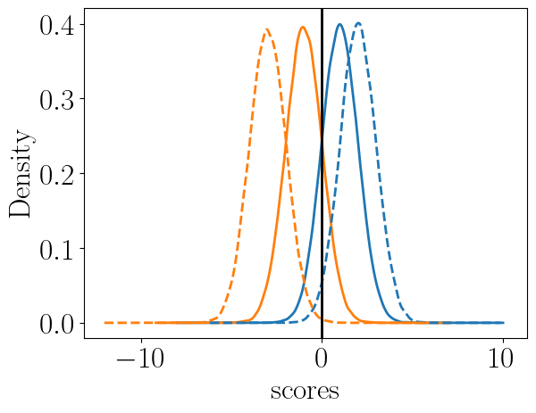
Figure 1. Synthetic true (solid lines) and predicted (dashed lines) score distributions for demographic two groups (orange and blue). The decision boundary at $\text{score}=0$ determines ground truth positive and negative labels based on the true scores, and predicted positive and negative labels based on the predicted scores. This simulates a situation in which the scoring algorithm overestimates the qualification of the advantaged group, and further disadvantages the disadvantaged group.

As a motivating example for the synthetic data experiment, let us consider credit scoring. Increasingly, scoring agencies are turning to ML to predict creditworthiness ((Langenbucher, 2020; Langenbucher and Corcoran, 2021)). Now imagine that a company predicts ML-based credit scores for candidates stemming from two protected groups only, for example for men and women (no non-binary persons applied). Candidates receiving a score equal or above 0 are labeled offered a credit contract, while those below are rejected.

4.1.1. Data set.

To model such a credit scoring situation, we generate a large synthetic data sets with 100,000 individuals and two demographic groups (one advantaged, e.g., male; and one disadvantaged, e.g., female) of approximately the same size. Each individual is assigned two scores, a true score, and a predicted score. The true score is to be understood as an individual’s true probability of being part of a desirable positive class (e.g., creditworthy person), while the predicted score is meant to represent a score that has been assigned to an individual by a (synthetic) scoring algorithm. They are sampled from a multivariate normal distribution with covariance matrix $[[1,0.8],[0.8,1]]$ and true score means $(1,-1)$ for the advantaged and disadvantaged groups, respectively. The corresponding predicted score means are $(2,-3)$. Additionally, we define a synthetic decision threshold to yield ground truth and predicted labels: those with a true (resp. predicted) score above zero are considered ground truth (resp. predicted) positive (i.e., creditworthy, and receive a credit offer). Conversely, those with a true (resp. predicted) score below zero are considered ground truth (predicted) negative (i.e., not creditworthy, and are rejected). Figure 1 depicts this data set. Blue lines correspond to the advantaged group, with both predicted scores (dashed blue line) and true scores (solid blue line) normally distributed with peaks greater than zero. Orange lines correspond to the disadvantaged group, with both predicted scores (dashed orange line) and true scores (solid orange line) normally distributed with peaks less than zero. This data set reflects a scenario of different base rates between the groups, as the advantaged group has a higher true probability of being positive. In our example, this is the male group. However, the scoring algorithm has overestimated the capabilities of the blue, advantaged group (the predicted score distribution is centered to the right of the true score distribution), and underestimated the capabilities of the orange, disadvantaged group (the predicted score distribution is centered to the left of the true score distribution). Additionally, the algorithm does a better job in predicting the true score distribution for the advantaged group, than it does for the disadvantaged group (the blue distributions overlap more). To emphasize the disparity between the two demographic groups, the advantaged group is 5.3 times more likely to be labeled positive based on the true scores, compared to 6250 times more likely to be labeled positive based on the predicted scores from the (unfair) scoring algorithm.

These two particular properties of disparities in model quality across groups are well studied in the algorithmic fairness literature ((Angwin et al., 2016; Zafar et al., 2017; Hardt et al., 2016)), which is why we choose this synthetic setting to present the functioning of FAIM. Note that we have plotted the true score distributions only for demonstration purposes to give a clear picture of the discriminatory scenario. They are usually not available, which is why FAIM relies on observable ground truth labels, as explained in Section 3.3.

Data set	Parameters	Performance			Error Rates
		Accur. ($\Delta$)	Precision ($\Delta$)	Recall ($\Delta$)	FPR ($\Delta$)	FNR ($\Delta$)
Synthetic	before FAIM	0.852	0.853	0.852	0.138	0.157
blue		0.860	0.868	0.860	0.869	0.002
orange		0.844	0.869	0.844	0.000	0.990
Synthetic	$\theta^{A}=1$	0.885 (0.033)	0.885 (0.033)	0.884 (0.032)	0.116 (-0.022)	0.114 (-0.043)
blue		0.884 (0.024)	0.873 (0.005)	0.884 (0.024)	0.560 (-0.309)	0.032 (0.032)
orange		0.885 (0.041)	0.874 (0.005)	0.885 (0.041)	0.032 (0.032)	0.557 (-0.433)
Synthetic	$\theta^{B}=1$	0.879 (0.027)	0.882 (0.029)	0.879 (0.027)	0.076 (-0.062)	0.166 (0.009)
blue		0.877 (0.017)	0.876 (0.008)	0.877 (0.017)	0.392 (-0.477)	0.073 (0.073)
orange		0.882 (0.038)	0.873 (0.004)	0.882 (0.038)	0.016 (0.016)	0.666 (-0.324)
Synthetic	$\theta^{C}=1$	0.865 (0.013)	0.873 (0.020)	0.865 (0.013)	0.208 (0.070)	0.062 (-0.095)
blue		0.854 (-0.006)	0.868 (0.000)	0.854 (-0.006)	0.918 (0.049)	0.001 (0.001)
orange		0.877 (0.033)	0.877 (0.008)	0.877 (0.033)	0.074 (0.074)	0.389 (-0.601)
Synthetic	$\theta^{A}=\theta^{B}=\theta^{C}$	0.883 (0.031)	0.883 (0.030)	0.883 (0.031)	0.137 (-0.001)	0.098 (-0.059)
blue		0.884 (0.024)	0.873 (0.005)	0.884 (0.024)	0.560 (-0.309)	0.032 (0.032)
orange		0.881 (0.037)	0.875 (0.006)	0.881 (0.037)	0.057 (0.057)	0.450 (-0.540)

Table 1. We report the performance metrics and error rates of the synthetic experiment after FAIM has been applied, and the corresponding relative improvements or deteriorations (green or red values in parenthesis, respectively). The first line always refers to the whole data set, whereas “blue” and “orange” contain results disaggregated by group. The top row shows metrics before FAIM has been applied.

4.1.2. Results.

Figure 2 shows the resulting score distributions of the synthetic data set after FAIM has been applied (left column), together with the corresponding transport maps that convert raw into fair scores (right column). The transport maps are to be read as follows: each raw score on the x-axis gets replaced by its corresponding value on the y-axis. Note that the transport maps necessarily differ by group, since the groups experience disparate treatment by our synthetic model which underestimated the capabilities of the disadvantaged group, and overestimated those of the advantaged. Each row of sub-figures corresponds to one of the scenarios described earlier. Consider Figures LABEL:fig:experiments:result:synthetic:condA and LABEL:fig:experiments:result:synthetic:TransportMapcondA as an example: they correspond to the experiment where we want to fully meet fairness criterion A). We see from the transport map (Fig. LABEL:fig:experiments:result:synthetic:TransportMapcondA), that the two score distributions are brought towards each other, as the disadvantaged group (orange) is assigned higher fair scores for the same raw scores. Figures LABEL:fig:experiments:result:synthetic:condB and LABEL:fig:experiments:result:synthetic:TransportMapcondB, as well as Figures LABEL:fig:experiments:result:synthetic:condC and  LABEL:fig:experiments:result:synthetic:TransportMapcondC, correspond to the experiments that fully implement the balance criteria B) and C), respectively. Note that these two balance criteria are defined only on a subset of individuals, i.e., the true negatives and the true positives, respectively. Thus, FAIM uses only this subset of the true negative (resp. true positive) individuals to calculate the transport maps and, in turn, the fair scores. This is reflected in Figures LABEL:fig:experiments:result:synthetic:condB and LABEL:fig:experiments:result:synthetic:condC: the fair score distributions overlap only for the truly negative (resp. positive) individuals, while the scores from the true positive (resp. negative) class are left untouched. Figures LABEL:fig:experiments:result:synthetic:compromise and  LABEL:fig:experiments:result:synthetic:TransportMapcompromise show the results of using the fairness objective $\theta^{A}=\theta^{B}=\theta^{C}=\frac{1}{3}$. We see that this setting indeed yields a compromise between the three fairness criteria.

Table 1 shows how FAIM affects classification performance and fairness. We understand fairness in terms of the three fairness objectives we seek to meet and therefore report metric and error rate differences in order to judge FAIM’s performance. The table reports the absolute values for each metric after FAIM has been applied, together with the changes relative to when FAIM is not applied (in parentheses). The top row shows the metrics before FAIM has been applied.

Observe the results for our first experimental setting with $\theta^{A}=1$. We expect an overall performance increase, as the algorithm calibrates the predictions with respect to actual ground truth evaluation. We also expect the effect to be more pronounced for the orange group, because of the larger error between predicted and ground truth scores for that group. Both expectations are confirmed in the results. The chance of the orange group to be labeled positive is now 5.7% of the blue group, which marks an improvement of more than two orders of magnitude.

Next, observe the results for the second and third fairness objectives where $\theta^{B}=1$, and $\theta^{C}=1$, respectively (balance criteria B) and C), respectively). When fulfilling criterion B), we expect the fair score distributions for ground truth negative individuals from the two groups to approximately match (recall Fig. LABEL:fig:experiments:result:synthetic:condB). Thus, the scores of ground truth negative blue and orange group individuals will decrease and increase, respectively. This corresponds to an FPR decrease for the blue group, which had a high base FPR including many false positive ground truth negative individuals scoring just slightly above the decision boundary whom become true negative after FAIM is applied. This also corresponds to either no or a slight FPR increase for the orange group, which had a base FPR of zero and ground truth negative individuals scoring far enough below the decision boundary that either none or only a few are mapped by FAIM above the decision boundary to become false positives. The results confirm our expectations. For the blue group, FAIM achieves an FPR of 39.2%, which marks an improvement w.r.t. the original FPR of 47.7%. We also see a slight increase of FPR for the orange group (1.6%). After FAIM is applied the FNR shows an improvement of 32.4%. Overall the probability of the orange group to receive a positive label is 5.3% of the blue group for $\theta^{B}=1$. When fulfilling criterion C), we expect the fair score distributions for true positive individuals to match (Fig. LABEL:fig:experiments:result:synthetic:condC), thus the false negative rates should improve, particularly for the orange group since most blue individuals were predicted positive by the original model. Again our expectations are confirmed by the results and declines in performance and error rates remain relatively small for both groups. Overall, the probability of the orange group for a positive label is 7.7% of the blue group.

(a)

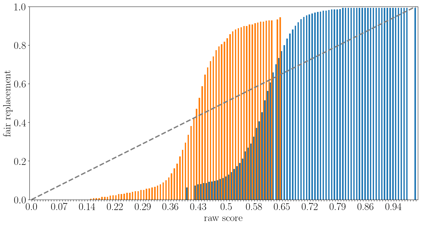
(b)

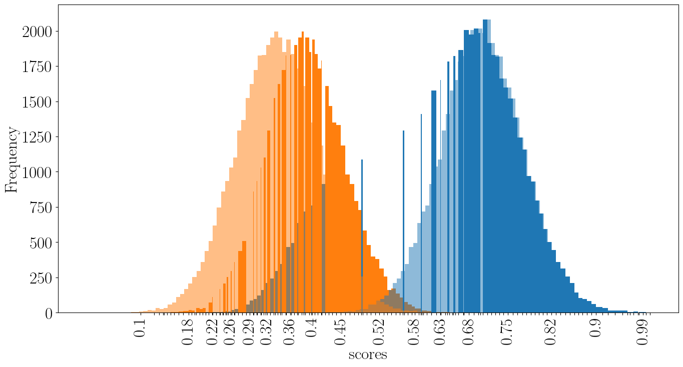
(c)

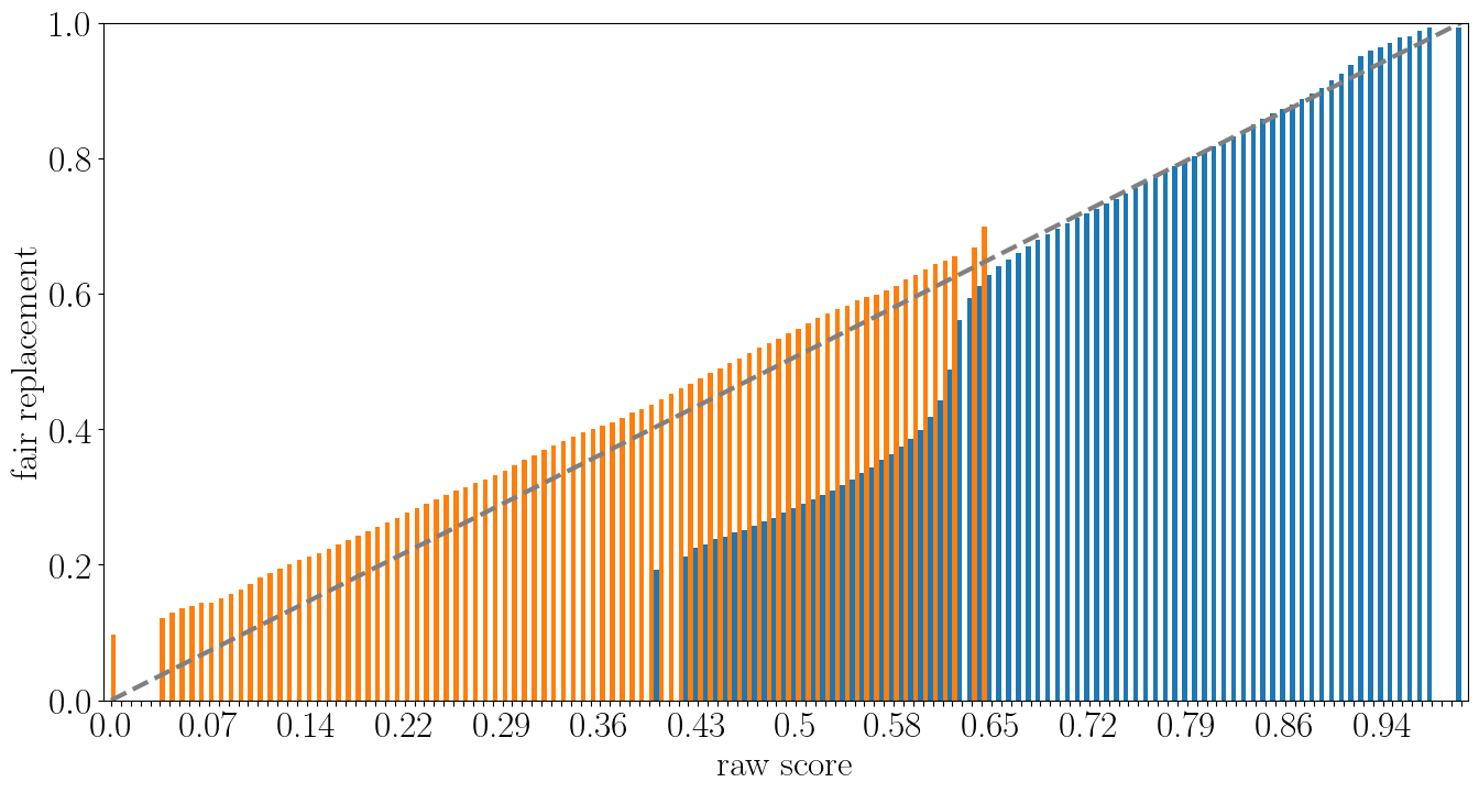
(d)

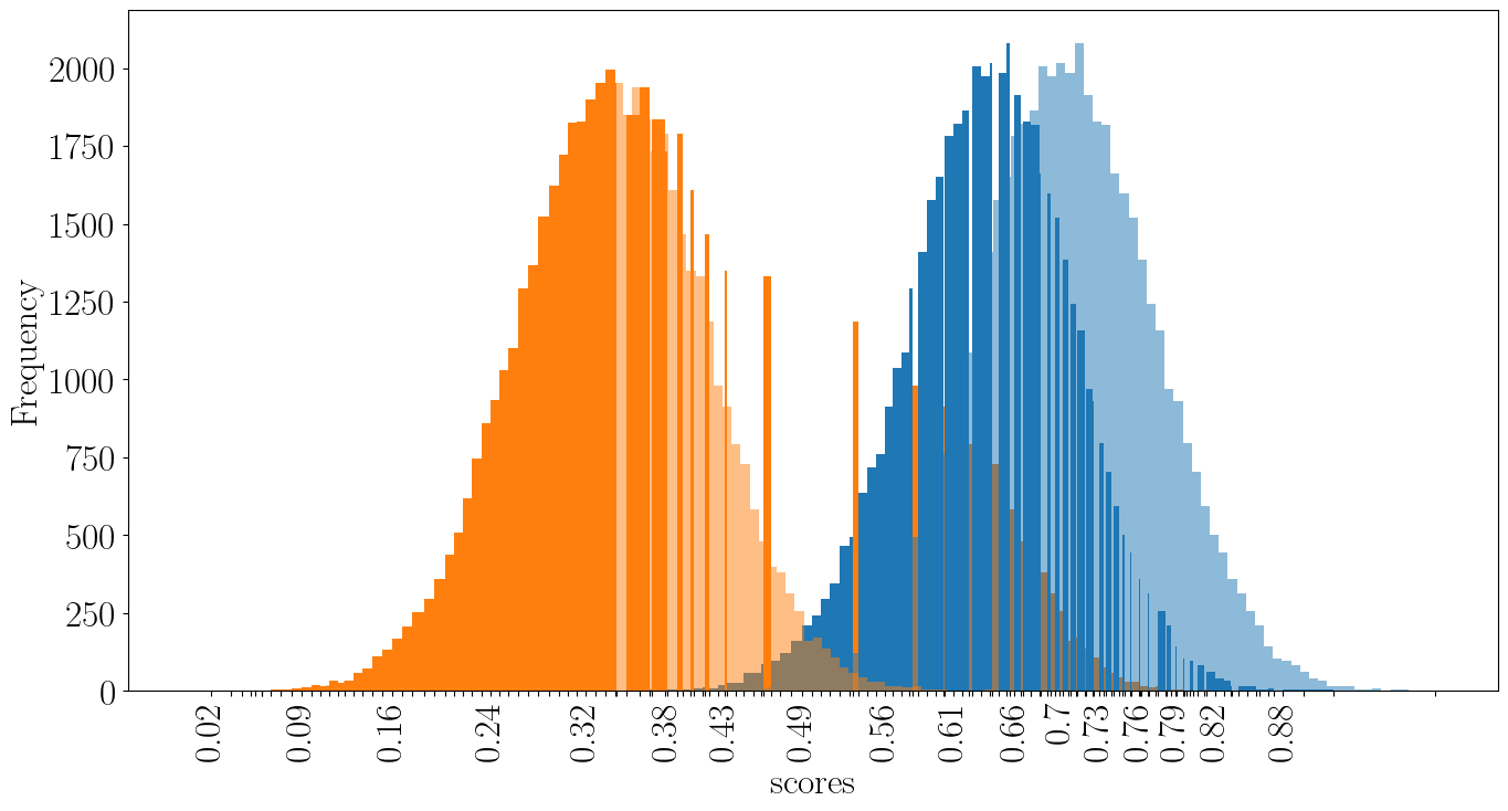
(e)

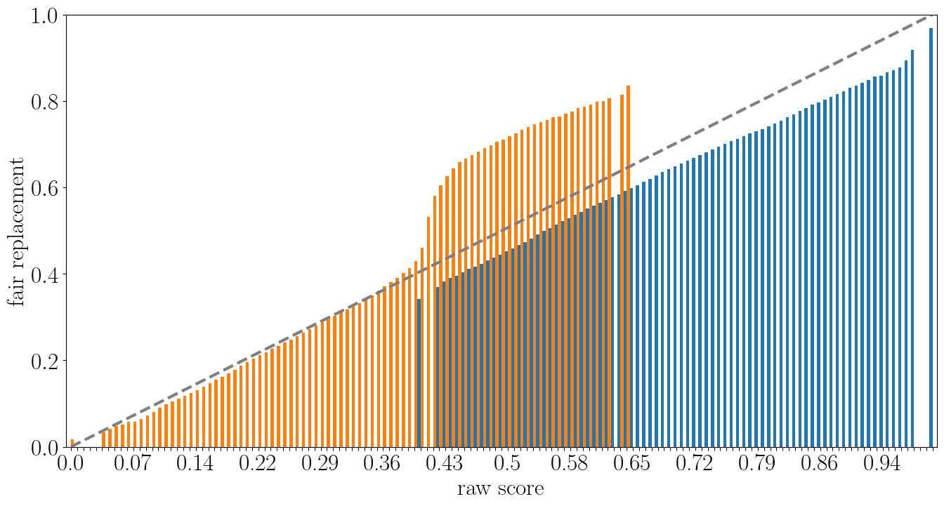
(f)

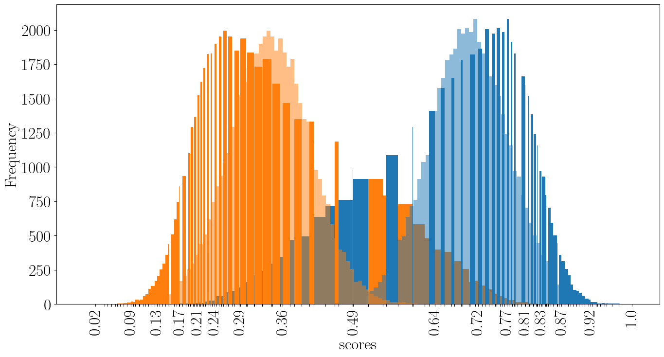
(g)

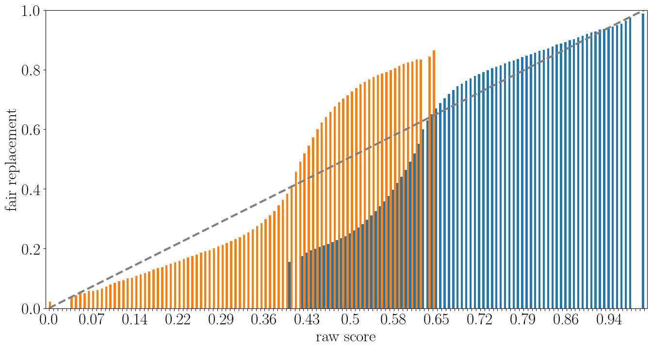
(h)

Figure 2. (Best seen in color). Left side: distributions of scores for each group after FAIM was applied under different fairness preferences (bold), together with the original distributions for comparison (transparent). Right side: transport maps that translate from the raw score (x-axis) to the respective fair score (y-axis). The gray dashed line marks the identity mapping. Note, that the two groups are assigned different fair scores for the same raw score. and that raw scores were normalized to $[0,1]$.

Last, observe the last experimental setting $\theta^{A}=\theta^{B}=\theta^{C}$, which corresponds to a compromise between the three mutually exclusive fairness criteria. As is confirmed by Figures LABEL:fig:experiments:result:synthetic:compromise and LABEL:fig:experiments:result:synthetic:TransportMapcompromise, the results in Table 1 show that FAIM yields a compromise between calibration, balance for the true negatives, and balance for the true positives. It achieves similar performance improvements as aiming for calibration only ($\theta^{A}=1$), but better FPR and FNR improvements. Compared to the balance criteria, this setting achieves better performance improvements, but only slightly worse FPR and FNR. Overall, the probability of the orange group to receive a positive label is 9.7% of the blue group for $\theta^{A}=\theta^{B}=\theta^{C}$.

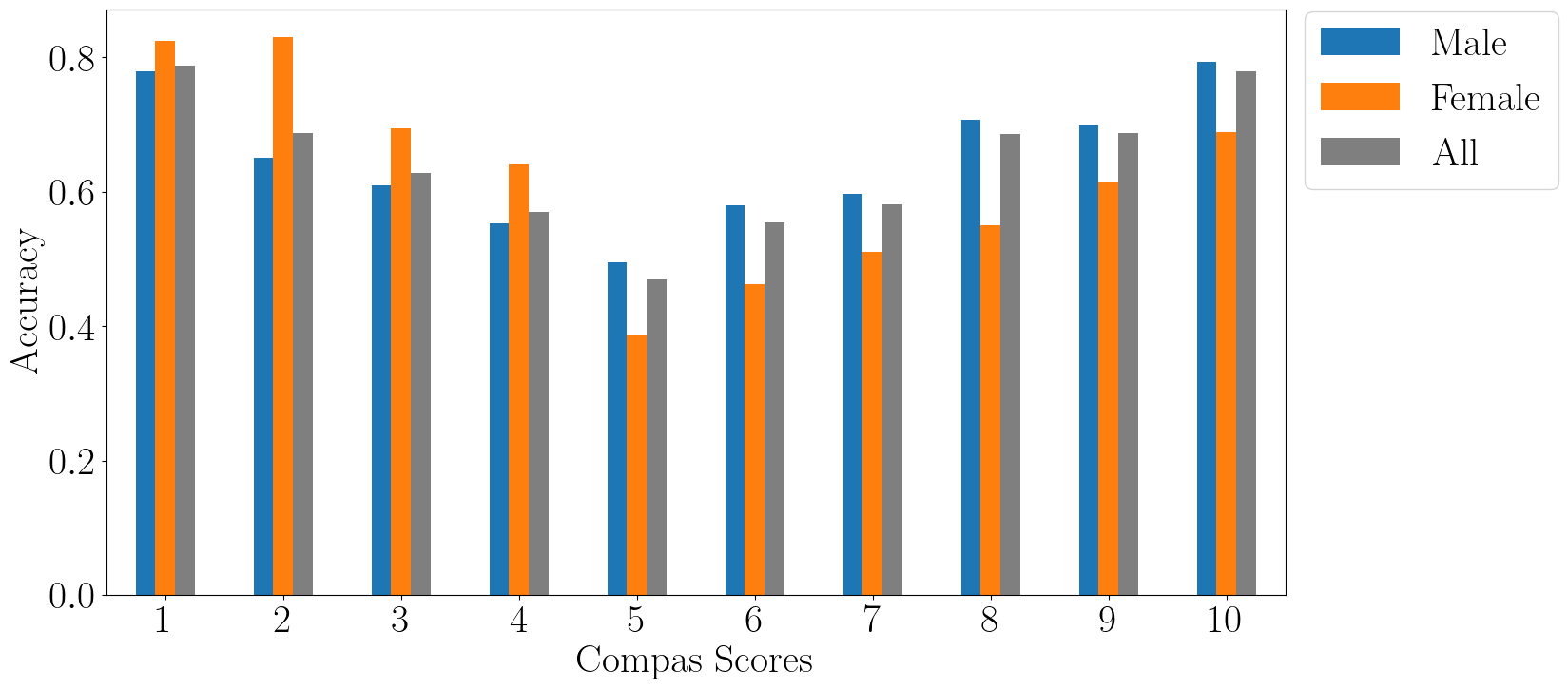
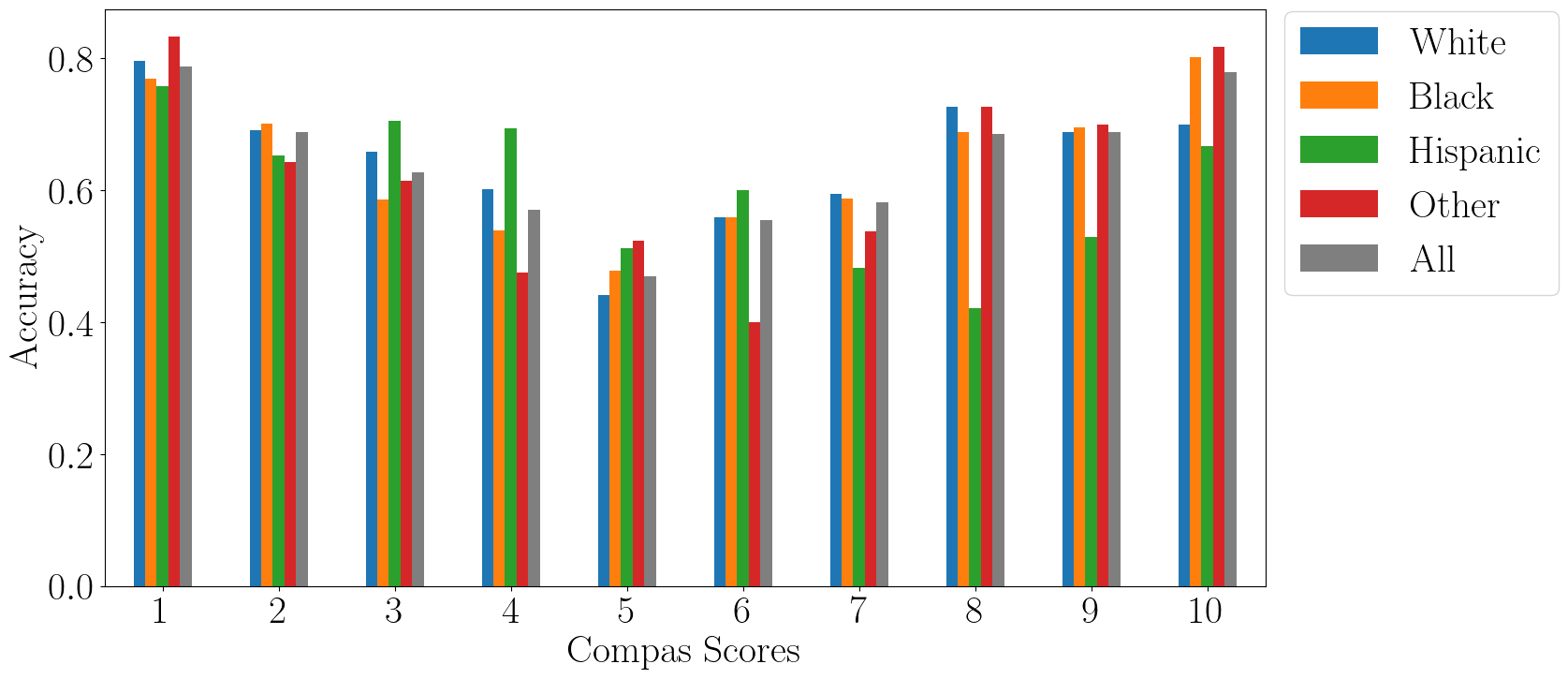
(i) Accuracy rates disaggregated by decile score and gender.

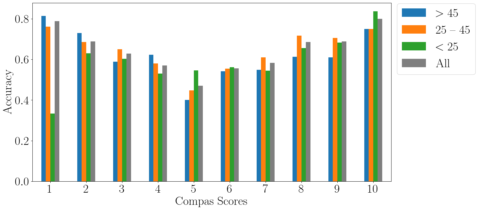
(j) Accuracy rates disaggregated by decile score and race.

(k) Accuracy rates disaggregated by decile score and age categories.

Figure 3. Accuracy rates disaggregated by COMPAS score. Across all demographics, accuracy rates show that the mid-range scores 4–7 do not provide very meaningful inside on recidivism risk.

4.2. Experiments on the COMPAS data set by (Angwin et al., 2016)

4.2.1. Data set

COMPAS (Correctional Offender Management Profiling for Alternative Sanctions) is a commercial tool developed by Northpointe, Inc. to assess a criminal defendant’s likelihood of recidivating within a certain period of time. Based on the promise to enhance fairness in judicial decision making, COMPAS is used in several US states as a decision aid for judges, e.g., in parole cases. In 2016, Angwin et al. (2016) published an analysis of the tool based on a data set of criminal defendants from Broward County, Florida, in which they found the tool to be biased against certain groups (more on this below).

From the data—as it was published by (Angwin et al., 2016)—we use decile_score (integers $\{1,2,...,10\}$) as predicted scores, and two_year_recid (boolean) as ground truth labels. Additionally, we construct groups based on sex, race, and age category using the features sex, race, and age_cat. To increase race group sizes, we merge races ‘Native American’ and ‘Asian’ into ‘Other’, leaving four race groups: ‘Caucasian,’ ‘African-American,’ ‘Hispanic,’ and ‘Other.’ These three features, i.e., the predicted score, the ground truth label, and the group, form the input for FAIM.

To assess the impact of FAIM on the predictive performance and the group error rates, we perform an analysis similar to that carried out by Angwin et al. (2016). We also translate the predicted score into a binary label of high and low risk corresponding to predicted score $\geq 5$ and $<5$, respectively. This binarization is applied to both the predicted scores from the COMPAS data set and the resulting fair scores produced by FAIM. Additionally, we calculate the probability of the disadvantaged groups to be assigned a high risk label relative to the advantaged group while correcting for the seriousness of their crime, previous arrests, and future criminal behavior.

4.2.2. Performance Analysis of the Original Model

To better interpret the results of applying FAIM to the COMPAS data set, we first provide a detailed performance analysis of the original COMPAS algorithm. Figure 3 shows the accuracy rates of the original model disaggregated by decile score and demographic group. Grey bars mark the accuracy rates measured for the aggregated data set. A striking insight is how poorly the model performs through the entire score range, but particularly for intermediate scores: within the range of 4–7, the accuracy rate for any demographic group hardly ever exceeds a level of 0.6. One could argue, of course, that a triangular pattern of accuracy rates (high accuracy for edge scores 0 and 10, lower accuracy for scores near the decision boundary of 5) would be expected from a well-calibrated model. After all, for a calibrated system, roughly 50% of individuals receiving a COMPAS score of 5 (corresponding to a normalized score of 0.5) would reoffend. Given that a COMPAS score $\geq 5$ corresponds to a prediction that an individual will reoffend, a calibrated system would achieve around 50% accuracy for the 5th score decile. It is important to understand however, that if the model was well-calibrated we would expect to see accuracy rates of at least 0.9 for scores 1 and 10, at least 0.8 for scores 2 and 8, and so forth, requiring an accuracy rate of at least 0.5 for score 0.5. As shown, the model never achieves any of these minimum performance rates for any demographic group.

Another interesting insight can be found by looking at the disparities of accuracy distributions across different demographic groups. Observe Figure 3: We see that women’s accuracy is higher than men’s in the lower scores, but vice versa for higher scores. This means that women are predominantly misclassified when they are assigned high scores, while men are predominantly misclassified, when they are assigned low scores. In other words, women are treated too harshly by the algorithm, while men are treated too gently (thus confirming the finding of Angwin et al. (2016)). The same is true for Hispanics in Figure 3, whose accuracy for the low scores is much higher than the one for the high score range. Surprisingly, Figure 3 reveals that young people, even though already being assigned relatively high scores, still seem to be treated too gently by the algorithm.

4.2.3. Experimental Results when Applying FAIM

Data set	Parameters	Performance			Error Rates
		Accur. ($\Delta$)	Precision ($\Delta$)	Recall ($\Delta$)	FPR ($\Delta$)	FNR ($\Delta$)
COMPAS	before FAIM	0.470	0.751	0.470	1.000	0.000
male		0.495	0.750	0.495	1.000	0.000
female		0.387	0.763	0.387	1.000	0.000
COMPAS	$\theta^{A}=1$	0.521 (0.051)	0.751 (0.000)	0.521 (0.051)	0.739 (-0.261)	0.185 (0.185)
male		0.495 (0.000)	0.750 (0.000)	0.495 (0.000)	1.000 (0.000)	0.000 (0.000)
female		0.613 (0.226)	0.763 (0.000)	0.613 (0.226)	0.000 (-1.000)	1.000 (1.000)
COMPAS	$\theta^{B}=1$	0.530 (0.060)	0.751 (0.000)	0.530 (0.060)	0.000 (-1.000)	1.000 (1.000)
male		0.505 (0.010)	0.750 (0.000)	0.505 (0.010)	0.000 (-1.000)	1.000 (1.000)
female		0.613 (0.226)	0.763 (0.000)	0.613 (0.226)	0.000 (-1.000)	1.000 (1.000)
COMPAS	$\theta^{C}=1$	0.530 (0.060)	0.751 (0.000)	0.530 (0.060)	0.000 (-1.000)	1.000 (1.000)
male		0.505 (0.010)	0.750 (0.000)	0.505 (0.010)	0.000 (-1.000)	1.000 (1.000)
female		0.613 (0.226)	0.763 (0.000)	0.613 (0.226)	0.000 (-1.000)	1.000 (1.000)
COMPAS	$\theta^{A}=\theta^{B}=\theta^{C}$	0.530 (0.060)	0.751 (0.000)	0.530 (0.060)	0.000 (-1.000)	1.000 (1.000)
male		0.505 (0.010)	0.750 (0.000)	0.505 (0.010)	0.000 (-1.000)	1.000 (1.000)
female		0.613 (0.226)	0.763 (0.000)	0.613 (0.226)	0.000 (-1.000)	1.000 (1.000)

Table 2. Evaluation of FAIM when applied to the COMPAS data set, disaggregated by gender. These are results only for an original COMPAS score of 5, because only individuals close to the decision boundary are reclassified after a score reassignment through FAIM. As such, for score ranges 1–4, and 6–10, neither error rates nor performance metrics change at all. Note also that, for one particular score, everybody is classified either positive or negative and the per-group error rates are thus either 0 or 1.

Our experimental results using FAIM on the COMPAS data set mostly confirm an important hypothesis: our algorithm cannot fix an inherently flawed model (garbage in, garbage out). As described earlier, we assessed accuracy, precision and recall, as well as false positive and false negative rates, total and disaggregated by demographics (similarly to results shown in Table 1). Because the nominal changes were negligible, we performed this same analysis disaggregated by COMPAS score (as in Fig. 3). Together with the analysis of the transport maps, this revealed the following: to fulfill fairness criteria B) and C), FAIM does not change the scores drastically. This is understandable since FAIM does not correct for accurate scores, but only for equal distributions, as soon as $\theta^{A}=0$. Thus, only few individuals with original scores of 4 or 5 get reclassified from low to high risk, and vice versa. Those with original scores 1–4, or 6–10, do not cross the decision boundary between the low and high risk class and therefore, none of the metrics changes for these score ranges.

Therefore, we exemplarily report results disaggregated by gender and for score 5 only in Table 2, to showcase the behavior of FAIM on the COMPAS data set. We see that the algorithm behaves as expected and does, in fact, improve performance and error rates the way we expect it to. However, since the original model performance is so low (see first row section in Table 2), we would recommend to rather abandon this model entirely. It seems futile to change random guessing into fair random guessing.

4.3. E-commerce data set from Zalando

4.3.1. Data set

For our last experiments, we use data from the e-commerce platform Zalando, one of Europe’s largest fashion and lifestyle retailers, operating in 25 European countries. We collected a data set of 81,048 articles on 27th October 2021, which belong to four different women clothes categories with a similar price range: skirts, jeans, trousers, and knitwear. Each data point contains the following information: a brand, a ranking score, and the number of impressions and clicks during the week after article collection. We look at the ratio of clicks over impressions and when it is above a certain threshold, assign a positive label to the article (as it got a positive weekly performance), or a negative label if it is below the threshold (as this article failed to gather enough clicks despite its visibility). Groups are assigned as follows: we compute a brand’s visibility as the average number of impressions per article for each brand and each category, and thus categorize brands having either low or high visibility. When this average is below the median, a brand is said to belong to the ‘low’ group, while if the number is above the third quartile, a brand is set to belong to the ‘high’ group. Articles of brands with visibility between the low and high group thresholds are discarded, leaving us with 62,461 articles. 70.5% of them belong to high visibility brands. Note, that the ranking scores are produced by a learning-to-rank model trained daily to optimize a surrogate normalized Discounted Cumulative Gain (nDCG) loss ((Järvelin and Kekäläinen, 2002)), but not to classify articles according to the ground truth labeling we defined above. However, because the nDCG relevance labels are based on customer interactions (i.e., implicit feedback), it is reasonable to assume that a good ranking model should be able to identify which article is likely to be clicked. Hence, the scores of an accurate click-through-rate classifier should provide a decent ranking. We observe in our data that, irrespective of whether those high articles are ground truth positive or negative, they receive higher scores than corresponding low articles. There are many reasons external to the ranking algorithm why customers would prefer well-known and highly visible brands: these brands have higher marketing budgets, they can afford a more aggressive pricing strategy thanks to economies of scale, and they benefit from the Matthew effect of accumulated advantage ((Perc, 2014)). Moreover, it is in the commercial interest of the platform to highlight such best selling items. At the same time, the platform may not want to reinforce the status quo but rather provide a level playing field for all brands to compete fairly. This makes it easier to attract new brands on the platform, offers a more diverse assortment to a potentially larger customer base, and can be seen as a good step to address the legal requirements discussed in 5.3.

Data set	Parameters	Performance			Error Rates
		Accur. ($\Delta$)	Precision ($\Delta$)	Recall ($\Delta$)	FPR ($\Delta$)	FNR ($\Delta$)
Zalando	before FAIM	0.624	0.623	0.192	0.079	0.808
high		0.586	0.622	0.238	0.122	0.762
low		0.717	0.747	0.012	0.002	0.988
Zalando	$\theta^{A}=1$	0.654 (0.030)	0.585 (-0.039)	0.518 (0.327)	0.252 (0.173)	0.482 (-0.327)
high		0.623 (0.038)	0.585 (-0.037)	0.604 (0.366)	0.361 (0.239)	0.396 (-0.366)
low		0.729 (0.012)	0.576 (-0.171)	0.186 (0.174)	0.055 (0.053)	0.814 (-0.174)
Zalando	$\theta^{B}=1$	0.621 (-0.003)	0.625 (0.001)	0.169 (-0.022)	0.070 (-0.010)	0.831 (0.022)
high		0.577 (-0.008)	0.625 (0.003)	0.189 (-0.050)	0.095 (-0.027)	0.811 (0.050)
low		0.725 (0.008)	0.623 (-0.124)	0.095 (0.083)	0.023 (0.021)	0.905 (-0.083)
Zalando	$\theta^{C}=1$	0.622 (-0.003)	0.623 (-0.001)	0.177 (-0.015)	0.073 (-0.006)	0.823 (0.015)
high		0.579 (-0.007)	0.625 (0.003)	0.196 (-0.043)	0.099 (-0.023)	0.804 (0.043)
low		0.725 (0.008)	0.608 (-0.139)	0.104 (0.092)	0.027 (0.025)	0.896 (-0.092)
Zalando	$\theta^{A}=\theta^{B}=\theta^{C}$	0.633 (0.009)	0.617 (-0.007)	0.259 (0.067)	0.110 (0.031)	0.741 (-0.067)
high		0.594 (0.009)	0.618 (-0.004)	0.294 (0.055)	0.153 (0.031)	0.706 (-0.055)
low		0.727 (0.010)	0.601 (-0.146)	0.124 (0.112)	0.033 (0.031)	0.876 (-0.112)

Table 3. We report the performance metrics and error rates of the experiment on Zalando data after FAIM has been applied, and the corresponding relative improvements or deteriorations (green or red values in parenthesis, respectively). The first line always refers to the whole data set, whereas “high” and “low” contain results disaggregated by group. The top row shows metrics before FAIM has been applied.

4.3.2. Results

From Table 3 we see that low visibility brands do indeed have a relative disadvantage over high visibility brands. The low recall, and the high false negative rate indicate that many relevant items from the low group are not shown to the customer. This situation is improved by FAIM in all four scenarios, albeit to varying degrees. Our results also show that the algorithm yields expected improvements: When criterion A) is desired, accuracy and recall is improved for both groups. Pursuing criterion B) or C) levels the respective error rates. Finally, a compromise between all three criteria is found when setting $\theta^{A}=\theta^{B}=\theta^{C}$.

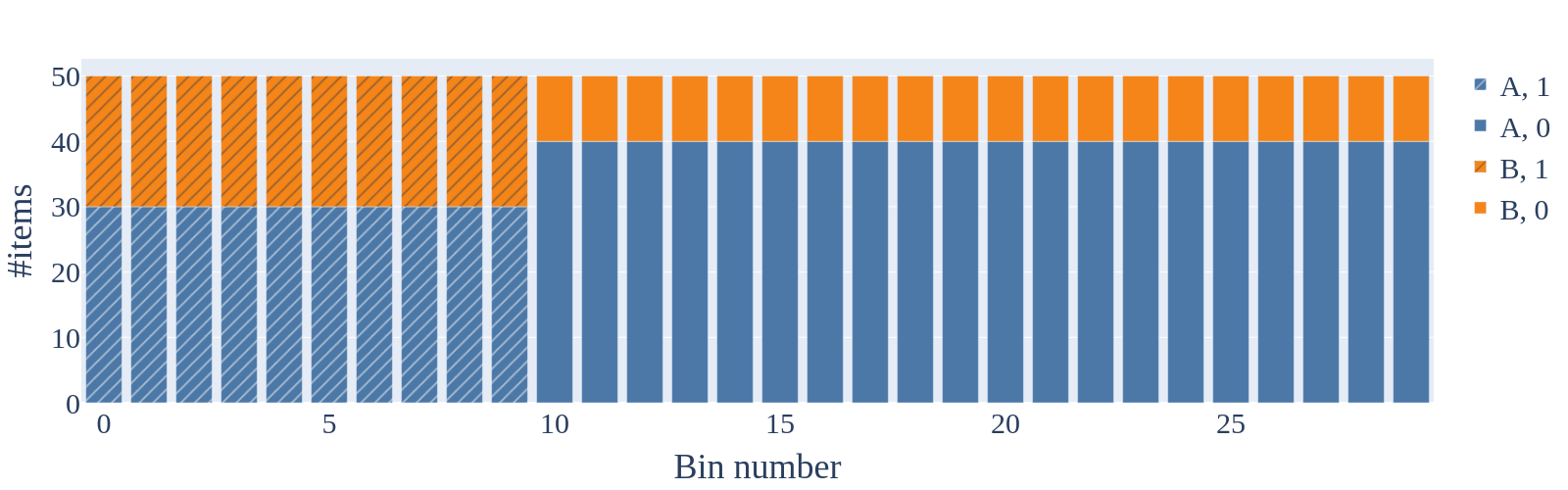
(a)

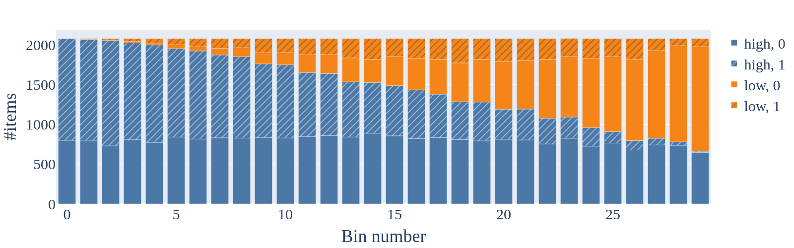
(b)

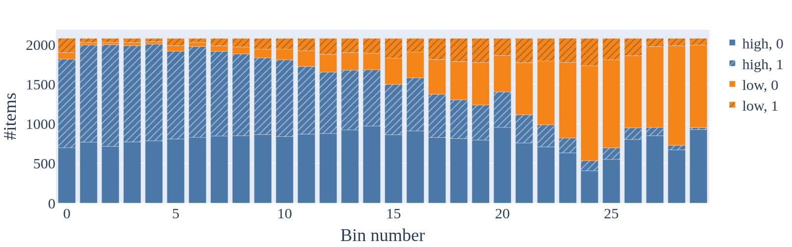
(c)

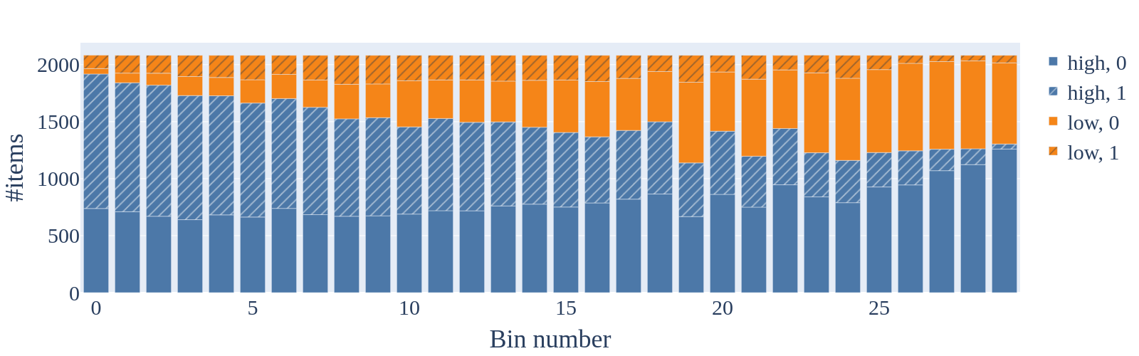
(d)

(e)

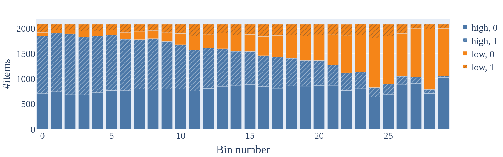
(f)

Figure 4. (Best seen in color). Product rankings with low and high visibility brands under different settings. Colors indicate group membership, stripes indicate a positive label, i.e., these are the products customers find more relevant. Fig. LABEL:fig:experiments:result:zalando:synthetic exemplifies an optimal outcome, where all relevant products are in the top positions, and the visibility of brands A and B is distributed according to their share of relevant products. Fig. LABEL:fig:experiments:result:zalando:real shows the distribution of relevant (and non-relevant) products from low and high brands as shown by Zalando’s ranking algorithm by the time of data collection. We see that famous brands do indeed have an advantage over less-known brands, as there are almost no products from the low group in the first few bins. Fig. LABEL:fig:experiments:result:zalando:condA—LABEL:fig:experiments:result:zalando:compromise show how the ranking changes after FAIM is applied with different values for $\theta^{A}$, $\theta^{B}$, and $\theta^{C}$. Depending on our preference for calibration, balance for the positive class, or balance for the negative class, we see varying degrees of visibility improvement for the low group.

For a better understanding on the effect of FAIM on the rankings, observe Figure 4. In Figure LABEL:fig:experiments:result:zalando:synthetic we show a fictive example for an ideal ranking: imagine a data set with two groups A and B. A has 1,000 items: 200 positive and 800 negative. B has 500 items: 300 positive and 200 negative. If we assume a perfect ranker, we can sort those items simply by their score. When we group them in bins of 50 items each, we would expect the first 10 bins to contain only positive items, and the next 20 bins to have only negative items. Furthermore, the positive bins should display a ratio of 300/200 for groups B and A respectively, while the negative bins should display a ratio of 200/800. Figure LABEL:fig:experiments:result:zalando:real shows the ranking as collected from the Zalando website on 27th October 2021, which by virtue of being real is not ideal. Since each bin contains more than 2,000 items, it is enough to focus on the first bins, as other items are shown very rarely, unless customers are actively looking for them. We see that the first five bins contain mostly high brands, meaning that relevant products from low brands are rarely shown to the customer, unless they start to use product filters or full text search. Again, there are various reasons why a customer would prefer well-known over less-known brands, but if we wanted to (or had to by legislation) mitigate the visibility disparities between high and low brands, FAIM provides a convenient approach (see Section 5.3 for a discussion on FAIM’s legal meaning for an e-commerce scenario such as ours). Figures LABEL:fig:experiments:result:zalando:condA– LABEL:fig:experiments:result:zalando:compromise show rankings after FAIM has been applied with different values for $\theta^{A}$, $\theta^{B}$, and $\theta^{C}$. In all cases, FAIM distributes visibility better across both brand groups, particularly for relevant products, which is the interesting case for an e-commerce platform such as Zalando.

5. Application of the Algorithm in Legal Scenarios

Given the contextual agility ((Wachter et al., 2021b)) of EU regulations with respect to the definition of fairness, it is advantageous to introduce a similar flexibility in the operationalization of fairness concepts. FAIM has a wide range of applications in scenarios in which the law compels the decision maker to make decisions in both an accurate and a non-discriminatory way. Technically speaking, this may result in a trade-off between competing fairness and accuracy measures embodying the contemplated criteria, i.e., calibration; balance for the negative class; balance for the positive class. Importantly, the weighting of the different measures via the $\theta$ interpolation parameters is a deeply normative choice which reflects competing visions of what is supposed to be considered fair, and legal, in a certain situation. Depending on the domain of application, the achievement of calibration, the balancing of false positives or of false negatives might be considered most important. FAIM affords the advantage of allowing the decision maker to flexibly adapt to these different scenarios by choosing different $\theta$ weights.

The broad discussion of different fairness metrics both in computer science and the law ((Wachter et al., 2021a; Hellman, 2020; Binns, 2018; Friedler et al., 2021; Kim, 2017; Pessach and Shmueli, 2020; Mitchell et al., 2021; Ghoash et al., 2021)) suggests that no single metric such as statistical parity, error balance or equalized odds will fit all contexts. This also applies to the fairness measures under discussion here ((Corbett-Davies and Goel, 2018)). As pointed out before, an important prerequisite for those metrics is the reliability of ground truth ((Bao et al., 2021)). If these data points are collected in a way that systematically disfavors one protective group, conditioning on ground truth data risks perpetuating imbalances included in them ((Bao et al., 2021; Wachter et al., 2021a; Chouldechova, 2017)). Within these constraints, ground truth measures like the ones underlying FAIM can nevertheless be helpful tools in many situations to capture normative desiderata, particularly if used alongside strategies to improve the correctness and representativeness of ground truth.

Generally speaking, choosing, for example, between a stronger balance for the negative or the positive class will depend on the respective consequences of misclassification (false negative and false positive predictions). As a result of prediction errors, individual and social costs arise, and legal norms may be violated. These costs and norms will differ widely depending on the deployment context. In the following, we review three examples in which different normative considerations may lead a decision maker to adopt varying weights for the respective accuracy and non-discrimination measures: recidivism prediction, credit scoring, and fair ranking according to the Digital Markets Acts (DMA).

5.1. Recidivism Prediction

In this paper, we consider recidivism prediction for technical and argumentative reasons: the original papers by Kleinberg et al. (2016) and Chouldechova (2017)showing incompatibility between fairness metrics did use the COMPAS case, and we directly build on their work. Hence, we use COMPAS as an example to clarify how FAIM works. However, when considering recidivism prediction, the first questions that arise from a juridical perspective are whether one legally may, or policy-wise should, use algorithmic tools such as the COMPAS model to assess recidivism risk in Criminal Justice proceedings at all (see also 6.3). We do not wish to make any claim as to the legitimacy of the usage of these tools in this paper; there are, if anything, good reasons to be quite skeptical about it. As mentioned, COMPAS is a proprietary model used in pretrial settings in the US to determine whether potential offenders should be detained until their trial, based on a prediction of recidivism likelihood. Similar models are currently employed in Canada, the UK, and Spain ((Watch, 2019, p. 122)). While the use of such instruments has sparked significant controversy, and critique, in the legal literature ((Starr, 2014; Mayson, 2019; Selbst, 2017; Katyal, 2019; Eaglin, 2017; Huq, 2019; Pruss, 2021)), courts such as the Wisconsin Supreme Court have condoned their use under certain safeguards, and their deployment is currently on the rise ((Hamilton, 2021); (Watch, 2019, p. 122)).

Within the scope of this paper, we cannot offer an in-depth discussion of the promises and perils of algorithmic recidivism risk assessment (see, e.g., (Solow-Niederman et al., 2019; Kleinberg et al., 2018), and 6.3). Rather, we would like to point out that, to the extent that such tools are used at all, they must clearly fulfill minimum requirements seeking to safeguard normative and legal principles of the jurisdictions in which they are deployed. Importantly, the impossibility theorems concerning various fairness metrics mentioned above apply equally in the case of algorithmic and human risk assessments. While the influence of fairness considerations on human risk predictions, for example by a judge, remains difficult to elucidate, FAIM allows to make the relevant trade-offs transparent and to rank the involved fairness metrics in varying degrees of priority.

In training the COMPAS model, the developers chose to prioritize calibration, which inevitably led to differing false positive and false negative rates given imperfect prediction and differing base rates between the involved ethnic groups ((Dieterich et al., 2016; Larson et al., 2016)). While accuracy remains significant in recidivism risk assessment—and is actually quite low with the COMPAS algorithm ((Dressel and Farid, 2018))—the core normative trade-off arguably occurs between the respective importance of equalizing false positive and false negative predictions. On the one hand, one could argue that the prevention of false positive outcomes should be prioritized because, under the rule of law, it is of utmost importance not to detain any person without sufficient reason. Under this reading, the greatest weight should be put on aligning false positive rates between groups, so that the burden of being unduly sent to prison is shared equally between the respective groups. On the other hand, one could claim that matching false negative predictions is crucial because they unduly spare individuals time in prison, affording a significant individual advantage to them. Under this reading, that undeserved benefit should not accrue to any protected group to a greater extent.

FAIM allows for the establishment of an intermediary position such that both balances, for the positive and the negative class, are fulfilled to an equal degree, even though only partially. To the extent that such instruments are used at all, and that the data they are based on are considered adequate, FAIM may therefore operationalize a policy compromise between factually irreconcilable goals.

From a different perspective, however, balancing false positives may be considered more important: losses loom larger than gains. Time in prison constitutes a highly significant restriction of personal freedom, interrupting private lives and careers, potentially endangering physical and mental health. Hence, lawmakers or judges may come to the conclusion that it is more important to share the burden of false positive predictions equally between groups than the unwarranted benefit of false negative predictions. FAIM then allows to prioritize the former criterion.

5.2. Credit Scoring

Entirely different normative considerations are present in the case of credit scoring. Imagine a bank uses an ML-based scoring algorithm to assess the creditworthiness of loan applicants, as in our synthetic experiment. Increasingly, ML is indeed used for these purposes ((Langenbucher, 2020; Langenbucher and Corcoran, 2021)). Here, accuracy facilitates so-called responsible lending, i.e., loan decisions in which the credit institution intends to ensure that the borrower is not overburdened by the repayment obligations. After the financial crisis of 2008/09, responsible lending has become a cornerstone of financial law. In the EU, for example, the obligation to lend responsibly is enshrined in Article 8 of the Consumer Credit Directive 2008/48/EC, and other EU law instruments install a comprehensive compliance and supervision regime demanding regular audits to ensure the accuracy of credit scoring models (Art. 174 et seqq. of the Capital Requirements Regulation 575/2013, CRR). Hence, accuracy should certainly receive significant weight in the case of credit scoring. As Art. 174(1) CRR puts it, statistical models used by banks need to have ‘good predictive power’.

However, with default base rates usually differing between protected groups, high degrees of calibration will lead to an imbalance in the false positive or false negative rates between the groups. A positive label, in credit scoring, means that the loan request is denied, a negative label that it is granted (because the risk of default is low enough). Clearly, false negative predictions may inflict financial damage on the lender if the credit cannot be repaid, but also potentially on the borrower, who may face financial penalties, eviction and future encumbrance due to a negative credit record. False positive predictions, on the other hand, give rise to opportunity costs: the lender does not earn interest payments, and the borrower does not obtain access to credit. Disparities concerning false negative or false positive rates affect access to credit or default rates between protected groups, and are therefore relevant for compliance with non-discrimination legislation.

In the EU, rules on indirect discrimination forbid even seemingly neutral practices putting protected groups at a particular disadvantage, unless these differences can be justified. Higher false positive rates clearly constitute a disadvantage for the affected group; even higher false negative rates can be viewed as a burden on the more often wrongly classified group, however, as they entail the concrete risk of default. Since accuracy and error rates cannot be balanced between protected groups at the same time under non-trivial conditions, the law will have to accept reasonable trade-offs between these competing and mutually exclusive obligations. It cannot and does not demand what is impossible (nemo ultra posse obligatur). From the perspective of legal doctrine, this will arguably take the route of the justification of a possible disadvantage. The damage inflicted must then be proportionate, given the reasons which can be advanced for prioritizing the other fairness criteria.

Given these preconditions, equalizing false negative credit predictions might be considered more important in the case of high-stakes loans (e.g., large sums and little collateral). Here, a default would be particularly disruptive, and hence that burden should be shared equally between protected groups. As a consequence, the $\theta$ weight of the balance for the positive class (Criterion C) should be higher than that for the negative class (Criterion B).

Conversely, in the case of low-stakes loans (e.g., low credit volume; sufficient collateral besides basic necessities of the borrower, e.g. beyond the house a family lives in; or limited personal liability in case of default), false positive predictions might be more deleterious than false negative ones because the damage is limited if the borrower defaults on the credit. Wrongfully denying access to credit may then have larger opportunity costs. Under such circumstances, the $\theta$ weight of the balance for the negative class (Criterion B) should be higher than that for the positive class (Criterion C). As an example, calibration could be set to 0.5, balance for the negative class to 0.35, and balance for the positive class to 0.15. Legally speaking, the fact that an unequal rate of false negative predictions persists will then arguably be justified by the overriding importance of aligning false positive predictions and calibration between groups.

5.3. Fairness in E-Commerce Rankings

Finally, our method may be used to implement emerging legal notions of fairness in e-commerce rankings. Particularly in EU law, a growing number of provisions aim to safeguard the impartiality of rankings in online contexts. At the most general level, these rules have shifted from the prohibition of self-preferencing via a focus on transparency to, so far, under-researched concepts of fairness in the Digital Markets Act (DMA). To the best of our knowledge, our contribution constitutes the first attempt to operationalize the fair ranking provisions of the DMA on both a technical and a legal basis.

5.3.1. Competition Law

The oldest and best-known rule of fairness in e-commerce rankings is derived from the prohibition, in general competition law, to abuse a dominant position (Art. 102 TFEU in EU law). It has long been argued that many dominant online undertakings, such as Google or Amazon, need to be scrutinized under this provision due to their dual role as providers of online marketplaces – on which third parties directly sell their goods to consumers – and as direct sellers of goods on their platforms ((Padilla et al., 2020; Graef, 2019)). Hence, such platforms may be considered competitors of the very business customers they serve on their marketplaces (vertical integration). As a consequence, dominant online platforms must not unduly preference their own offers vis-à-vis those of their business customers in rankings they display as a result of consumer search queries. This rule has led to some of the most spectacular fines in recent EU competition law. For example, the General Court of the European Union, in November 2021, affirmed the 2017 decision by the EU Commission to fine Google with €2.4 billion for engaging in self-preferencing in its online comparison shopping service. A similar issue is at stake in the Amazon buy box case, in which the Italian Competition Authority, in December 2021, imposed a record fine of €1.1 billion on several Amazon companies for tying access to the buy box to the use of Amazon’s own logistics channel (Fulfillment by Amazon).

The upshot of these rulings is that dominant platforms which serve a dual role of marketplace and seller must abstain from systematically tweaking their rankings to their own benefit. This rule against self-preferencing, deduced from Art. 102 TFEU and pertinent case law, may be considered a first substantive fairness element for the order of the ranking itself ((Podszun and Bongartz, 2021)). However, it only applies to undertakings which dominate a certain market.

5.3.2. Transparency

Often, though, it is difficult for outsiders, even for the business customers, to determine how these rankings come about. Two new provisions therefore install explicit transparency provisions for rankings in EU law ((Hacker and Passoth, 2022; Eifert et al., 2021)). First, Art. 5 of the so-called P2B (Platform to Business) Regulation (EU) 2019/1150 obliges online intermediaries and search engines, independent of their market power, to disclose the main parameters of ranking and their relative importance. The provision has been in effect since July 2020. It is supposed to foster the predictability and understanding of the ranking for business users, and to foster competition between different intermediaries with respect to the ranking parameters (Recital 24 of the P2B Regulation). In a similar fashion, second, the new Art. 6a of the Consumer Rights Directive (CRD) has required online marketplaces from the end of May 2022 on to divulge to consumers the main parameters for rankings based on consumer search queries as well as their relative importance. According to the new Art. 2(1)(n) of the Unfair Commercial Practices Directive, ‘online marketplace’ denotes any software operated by or on behalf of a trader which allows consumers to conclude distance contracts with other traders or consumers. Therefore, the rule does not apply to companies only selling goods directly to consumers, but is again independent of market power.

Essentially, scholars have argued, these provisions introduce an obligation for the global explanation of the ranking model ((Hacker and Passoth, 2022; Grochowski et al., 2021)). It may be fulfilled, for example, by using interpretable machine learning models (e.g., linear or logistic regression ((Rudin, 2019))) or by using global post-hoc explanations for black box models (e.g., DNNs) such as an average over local SHAP values ((Lundberg and Lee, 2017)) or SpRAy ((Lapuschkin et al., 2019)). However, the provisions do not add any specific, substantive fairness criteria concerning the order of the ranking itself.

5.3.3. The EU Digital Markets Act

The DMA, which will come into effect in the EU in 2023, takes these existing provisions yet one step further by introducing a novel fairness condition for rankings. Its importance is hard to overstate: failure to comply with the DMA provisions may be sanctioned by fines of up to 10% of the global annual turnover of the offender (Art. 30(1) DMA), and up to 20% in the case of a repeated violation (Art. 30(2) DMA). The DMA includes a whole range of provisions aimed at strengthening contestable markets and fair competition in online environments by designing specific rules applicable to so-called gatekeepers, in essence large online platforms.

Fairness in the DMA.

Art. 6(5) DMA specifically tackles rankings, including when delivered via a virtual assistant (Recital 51 DMA; for example, a personal voice assistant). Art. 6(5) DMA first reiterates the prohibition of self-preferencing known from general antitrust law.

The second sentence of Art. 6(5) DMA starts by specifying that rankings need to be transparent. As Recital 52 suggests, this could refer to the transparency provisions of the P2B Regulation. Importantly, Art. 6(5) DMA goes on to demand that gatekeepers must, in general, apply ‘fair and non-discriminatory conditions’ to their rankings. In the legal space, this has sparked a discussion on how these criteria may be interpreted ((Brouwer, 2021; Hacker, 2022b)). So far, however, no clear guidance or consensus has emerged on what these additional fairness requirements for rankings under the DMA could mean for gatekeepers.

This raises the question of how the obligation to apply fair and non-discriminatory conditions to rankings could be interpreted. We cannot explore this conceptual issue in depth in this paper. If, however, courts concluded in the future that fairness and non-discrimination under the DMA clause was somehow linked to accuracy, false positives and false negatives, we can smoothly operationalize the DMA fairness condition with FAIM. This is significant insofar as previous discussions of fairness in algorithmic contexts have invariably focused on non-discrimination law ((Zehlike et al., 2017; Asudeh et al., 2019; Singh and Joachims, 2018; Zehlike et al., 2022b)), and not on fairness conditions in e-commerce regulation, such as the DMA.

DMA Ranking with FAIM.

FAIM allows to specifically and flexibly re-order gatekeeper rankings such that certain conditions are prioritized, depending on the exact, and as of yet unknown, binding interpretation of Art. 6(5) DMA. In the case of e-commerce rankings, one hypothetical interpretation by courts could be that accuracy as well as an equal false positive rate are the most important parameters among the three conditions. Under such a reading, false negative predictions might be considered less important than false positive predictions as most consumers will not even see or engage with those items which are ranked at low positions. If a platform, preemptively or as a result of a court or agency order, wishes to avoid that criteria such as incumbent status play a role in the top-ranked products, $\theta$ values can be set accordingly. They could, for example, convey high priority to equalizing the false positive rate (Criterion B) between high-visibility and low-visibility brands.

A second hypothetical interpretation would focus on false negatives. False negative predictions unduly demote products in the ranking and thus deprive affected items of visibility and hence of transactions. If a regulatory agency or court found that the false-negative rate needs to be balanced between certain groups, FAIM can again be tuned to implement such a requirement by choosing corresponding $\theta$ values (high values for Criterion C).

In future work, we will seek to identify further distinctions which may be problematic under the DMA fairness clause and which may be remedied by FAIM. Importantly, the fairness clause in the DMA provides an opportunity to reflect upon fairness criteria in e-commerce rankings beyond general non-discrimination law and the prohibition of self-preferencing in competition law.

6. Discussion and Limitations

6.1. Normative Choices and Applicability

To explicitly name the normative choices FAIM implies, we use the concepts by  Friedler et al. (2021) of two different metric spaces—construct space and observable space. Construct space denotes an idealized reality in which all feature values are correctly registered, and a decision is based on those features. However, decision makers usually do not have access to this realm of an objective truth. Rather, they need to base their model on observable space, which contains the feature values the decision maker has access to via measurement., and the decisions based on them. Importantly, ground truth may correctly reflect, or at least closely approximate, construct space—or it may not. This implies a first limitation for our method. FAIM operates in observable space, and does not undo any harm that might arise from a potentially biased mapping between construct and observable space, e.g., by systematic measurement errors. This is because we obtain our ground truth labels from observing behavior of scored individuals, such as: “did someone who was labeled creditworthy actually repay the loan?” Such observations naturally incorporate historic and on-going discrimination, as they usually do not ask: “If a person who was labeled creditworthy did not repay the loan, was that because she can genuinely not handle money, or because she belongs to a disadvantaged group?” To be sure, this question is crucial for the societal mitigation of discrimination in the long term. However, with the data we have at our disposition, we usually cannot answer it exhaustively. Hence, FAIM must generally content itself with correcting unequal calibration or disparate error rates, defined by a divergence from ground truth, that disproportionately affect a certain group of individuals. As such disparities often correlate with the membership of a disadvantaged group in society, it may also correct discrimination caused by skewed mappings between construct and observable space to a certain extend (as we have seen in our experimental results). However, this is only a side-effect and depends on the nature of discrimination that is present in the data. If ground truth is close to reality, i.e., to construct space, then we can cure biased mappings between construct and observable space; otherwise, not. For the same reasons, FAIM addresses technical and emergent, but not pre-existing bias, as defined by Friedman and Nissenbaum (1996).

We therefore advise FAIM to be used in settings where ground truth observations are sufficiently reliable (though this is a necessary condition for any data-driven decision making), and it can be assumed that groups can be meaningfully compared by the respective measures of qualification or quality. As an example for a non-comparable qualification measure across genders, consider the h-index ((Hirsch, 2005)), which suffers from strong gender bias. Research shows that women, for the same amount and quality of research, receive significantly lower h-index values because it takes them longer to publish, and their work is less cited than men’s ((Caplar et al., 2017)). In cases where groups cannot be meaningfully compared, a method that implements statistical parity or other affirmative action policies independent of ground truth (such as FA*IR by Zehlike et al. (2017, 2022a)) is an appropriate choice (see also (Wachter et al., 2021a)).

6.2. Limitations of FAIM

Continuous Mathematical Framework.

As stated, we work with a continuous scale of possible scores (in the real interval $[0,1]$) and accordingly with continuous probability distributions. In practice, of course, there will be only a discrete set of possible scores, and a finite set of individuals under scrutiny. The reason we work in a continuous setting is of a mathematical nature, in that it allows us to use certain tools from the theory of optimal transport, which in a discrete setting would complicate the theory considerably. It is common and reasonable practice to approximate discrete models by continuous ones, as long as the number of individuals considered is large and their scores are sufficiently spread out over a finite scale. Thus, our framework would not be suitable for a situation where there are only very few possible score values, e.g., only three or four. Further discussion in this direction, for a related problem, can be found in Zehlike et al. (2020).

Discontinuities in score distribution.

In criterion B) (we use this case as an example to explain the problem, but the same applies to criterion C), we only balance the scores for the negative class and ignore the true positives. This means that the scores of the true positives remain unchanged by FAIM. This might become a problem for rare scores of true negative individuals for whom there was no example in the data when calculating the optimal transport (OT) matrix. Remember that our algorithm calculates an optimal transport matrix to translate raw scores into fair scores for previously unseen individuals. This means that for new data points, we do not know the ground truth label. Instead, FAIM consults the OT matrix that corresponds to a certain group and setting of $\theta$ and checks if it finds a raw score entry in that matrix. In such a case, the following scenario might arise when trying to optimize for criterion B) only: Suppose a true negative person’s score lies at the edge of the overall true negative score distribution, i.e., only few others (in the world) have the same score while being true negative. In addition, critically, no true negative person had this score when the OT matrix was computed. In this case, the algorithm does not have an entry for translation in the OT matrix. As a result, this individual would be considered true positive, and their score would be left untouched.

6.3. Critique of using COMPAS as an experimental scenario

Bao et al. (2021) raise the problem that Risk Assessment Instrument (RAI) data sets such as COMPAS are used for benchmarking fairness methods in a purely technical fashion without recognizing the domain- and data-specific concerns of Criminal Justice (CJ). As a result, technical fairness method contributions could be interpreted as substantive interventions in the CJ domain. However, the authors rightly argue, the latter presupposes careful considerations of the domain specifics that may invalidate such results. They raise several serious concerns about COMPAS: outcome label bias due to construct invalidity; measurement bias that cannot be calibrated due to lack of (reliable) ground truth; protected attribute measurement bias; racial bias in covariates; and distribution issues due to label selection bias. We recognize and acknowledge the concerns raised by Bao et al. However, since our contribution is an improvement on a previously published method presented on the COMPAS data set, we deem it important to enable a comparison of our results with the original. Thus, we publish the results from our experiments on the COMPAS data set only as a technical comparison with the results in Kleinberg et al. (2016), and under the caveat that reliable ground truth is not available for the COMPAS data set. Hence, the results on applying FAIM to COMPAS are not intended as a contribution to real-world outcomes in the criminal justice domain. Rather, we discuss how FAIM could be used in a pretrial setting if the model and data were considered adequate.

6.4. Data Missingness

Data missingness is a validity concern for the study of any fairness criterion, as noted by Goel et al. (2021), and is not unique for FAIM. As is the case for many fairness criteria, FAIM assumes the availability of ground truth data that is representative of the underlying distribution, and the absence of systematic censorship ((Kallus and Zhou, 2018)) in the data generation process. If systematic censorship occurs due to biased decision making, then this prevents us from sampling from the ground truth distribution needed for an unbiased fairness criterion, thus making evaluation problematic.

Concerning the three data sets used in this paper: as mentioned, we use the COMPAS data set to allow a direct comparison with the metric proposed by Kleinberg et al. (2016), and we thus do not want to modify the data set, for example through recovery or imputation. As shown by Goel et al. (2021), it is possible to recover parts of the distribution on certain assumptions about the causal structure of the decision-making process, but making such assumptions would not allow comparison with the results of Kleinberg et al. (2016) or allow us to make any general conclusions about applying FAIM to COMPAS.

The e-commerce data set is subject to systematic censorship in the sense that articles classified as ”low visibility” would receive less exposure and thus do not have opportunities to gain more exposure. Modifying the exploration-exploitation strategy for the learning to rank model would allow us to sample from the missing data to a larger degree, but performing such experiments would be prohibitively costly.

Finally, to further investigate the effect of data missingness on FAIM, we could introduce synthetic missingness to the synthetic data set, but would have to do so under the assumption of different causal structures, which are in an undefined and infinite search space. Thus, it is unclear what the relevant causal structures would be that would allow us to make meaningful conclusions.

7. Conclusion

In this paper, we have presented FAIM, a re-scoring algorithm that interpolates between three important criteria from the literature on fairness in machine learning: calibration, balance for the negative class, and balance for the positive class. Previous research has shown that they are mutually exclusive under reasonable factual assumptions. However, in many practical and legal scenarios, it is unsatisfactory to fully prioritize one criterion while neglecting the other two.

FAIM allows to find an optimal compromise between the three criteria through three per-group parameters $\theta^{A},\theta^{B}$, and $\theta^{C}$ using optimal transport theory. The parameter settings can be flexibly adapted to various scenarios. In this way, decision makers can balance competing interests and rights of protected groups; and they may adapt one model to different legal requirements. We presented mathematical theory together with a pseudocode implementation to help readers with different backgrounds to follow our approach. The model was tested in extensive experiments on real-world data sets from the criminal justice and the e-commerce domain. Our experiments have shown that FAIM is effective under all scenarios, but that an inherently flawed model or data set should not be “fixed” via fairness constraints. As such, we want to stress that our model is not a means of ethical reasoning, i.e., it can not determine whether a candidate should or should not receive bail or credit, or whether a product should be included in a top-$k$ ranking. Instead, it ensures an optimal compromise for mutually exclusive fairness constraints according to the desires of a decision maker, expressed through the choices of $\theta^{A},\theta^{B}$, and $\theta^{C}$.

However, we also stressed that any choice of $\theta$ values must, of course, remain within the confines of the law. Hence, we discussed how FAIM may be harnessed to comply with competing legal non-discrimination obligations in three concrete settings corresponding to our experiments: credit scoring, bail decisions, and emerging notions of fairness in e-commerce rankings. The discussion shows that our model can handle both traditional legal fields and novel obligations under the recently enacted DMA. To our knowledge, our paper is the first to explore the DMA from both a technical and a legal perspective.

8. Acknowledgments

We want to thank Geraud Le Falher and Pak-Hang Wong for their support and insightful suggestions to improve the paper. The authors do not have any funding to disclose other than their affiliation.

References

- (1)
- Agueh and Carlier (2011) Martial Agueh and Guillaume Carlier. 2011. Barycenters in the Wasserstein space. SIAM Journal on Mathematical Analysis 43, 2 (2011), 904–924.
- Ambrosio and Gigli (2013) Luigi Ambrosio and Nicola Gigli. 2013. A user’s guide to optimal transport. In Modelling and optimisation of flows on networks. Springer, 1–155.
- Angwin et al. (2016) Julia Angwin, Jeff Larson, Surya Mattu, and Lauren Kirchner. 2016. Machine bias. ProPublica, May 23, 2016 (2016), 139–159.
- Asudeh et al. (2019) Abolfazl Asudeh, HV Jagadish, Julia Stoyanovich, and Gautam Das. 2019. Designing fair ranking schemes. In Proceedings of the 2019 International Conference on Management of Data. 1259–1276.
- Bao et al. (2021) Michelle Bao, Angela Zhou, Samantha Zottola, Brian Brubach, Sarah Desmarais, Aaron Horowitz, Kristian Lum, and Suresh Venkatasubramanian. 2021. It’s COMPASlicated: The Messy Relationship between RAI Datasets and Algorithmic Fairness Benchmarks. arXiv preprint arXiv:2106.05498 (2021).
- Barocas and Selbst (2016) Solon Barocas and Andrew D Selbst. 2016. Big data’s disparate impact. Calif. L. Rev. 104 (2016), 671.
- Bellogín et al. (2017) Alejandro Bellogín, Pablo Castells, and Iván Cantador. 2017. Statistical biases in information retrieval metrics for recommender systems. Information Retrieval Journal 20, 6 (2017), 606–634.
- Berk et al. (2021) Richard Berk, Hoda Heidari, Shahin Jabbari, Michael Kearns, and Aaron Roth. 2021. Fairness in criminal justice risk assessments: The state of the art. Sociological Methods & Research 50, 1 (2021), 3–44.
- Binns (2018) Reuben Binns. 2018. Fairness in Machine Learning: Lessons from Political Philosophy. In Conference on Fairness, Accountability and Transparency. 149–159.
- Bono et al. (2021) Teresa Bono, Karen Croxson, and Adam Giles. 2021. Algorithmic fairness in credit scoring. Oxford Review of Economic Policy 37, 3 (2021), 585–617.
- Brenier (1987) Yann Brenier. 1987. Décomposition polaire et réarrangement monotone des champs de vecteurs. CR Acad. Sci. Paris Sér. I Math. 305 (1987), 805–808.
- Brenier (1991) Yann Brenier. 1991. Polar factorization and monotone rearrangement of vector-valued functions. Communications on pure and applied mathematics 44, 4 (1991), 375–417.
- Brouwer (2021) Dennis Jeroen Brouwer. 2021. Towards a ban of discriminatory rankings by digital gatekeepers?: Reflections on the proposal for a Digital Markets Act. Internet policy review (2021).
- Cabral et al. (2021) Luis Cabral, Justus Haucap, Geoffrey Parker, Georgios Petropoulos, Tommaso M Valletti, and Marshall W Van Alstyne. 2021. The EU digital markets act: a report from a panel of economic experts. Publications Office of the European Union (2021).
- Calders and Žliobaitė (2013) Toon Calders and Indrė Žliobaitė. 2013. Why unbiased computational processes can lead to discriminative decision procedures. In Discrimination and privacy in the information society. Springer, 43–57.
- Caplar et al. (2017) Neven Caplar, Sandro Tacchella, and Simon Birrer. 2017. Quantitative evaluation of gender bias in astronomical publications from citation counts. Nature astronomy 1, 6 (2017), 1–5.
- Chiappa et al. (2020) Silvia Chiappa, Ray Jiang, Tom Stepleton, Aldo Pacchiano, Heinrich Jiang, and John Aslanides. 2020. A General Approach to Fairness with Optimal Transport.. In AAAI. 3633–3640.
- Chiappa and Pacchiano (2021) Silvia Chiappa and Aldo Pacchiano. 2021. Fairness with Continuous Optimal Transport. arXiv preprint arXiv:2101.02084 (2021).
- Chouldechova (2017) Alexandra Chouldechova. 2017. Fair prediction with disparate impact: A study of bias in recidivism prediction instruments. Big data 5, 2 (2017), 153–163.
- Corbett-Davies and Goel (2018) Sam Corbett-Davies and Sharad Goel. 2018. The measure and mismeasure of fairness: A critical review of fair machine learning. arXiv preprint arXiv:1808.00023 (2018).
- Dawid (1982) A Philip Dawid. 1982. The well-calibrated Bayesian. J. Amer. Statist. Assoc. 77, 379 (1982), 605–610.
- De Vries (2013) Sybe A De Vries. 2013. Balancing fundamental rights with economic freedoms according to the European Court of Justice. Utrecht Law Review 9, 1 (2013), 169–192.
- Dieterich et al. (2016) William Dieterich, Christina Mendoza, and Tim Brennan. 2016. COMPAS risk scales: Demonstrating accuracy equity and predictive parity. Northpointe Inc. (2016).
- Dignum (2019) Virginia Dignum. 2019. Responsible artificial intelligence: how to develop and use AI in a responsible way. Springer Nature.
- Dressel and Farid (2018) Julia Dressel and Hany Farid. 2018. The accuracy, fairness, and limits of predicting recidivism. Science advances 4, 1 (2018), eaao5580.
- Dwork et al. (2012) Cynthia Dwork, Moritz Hardt, Toniann Pitassi, Omer Reingold, and Richard Zemel. 2012. Fairness through awareness. Proceedings of the 3rd innovations in theoretical computer science conference, 214–226.
- Eaglin (2017) Jessica M. Eaglin. 2017. Constructing Recidivism Risk. Emory Law Journal 67, 1 (2017), 59–122.
- Ebers et al. (2021) Martin Ebers, Veronica RS Hoch, Frank Rosenkranz, Hannah Ruschemeier, and Björn Steinrötter. 2021. The European commission’s proposal for an artificial intelligence act—a critical assessment by members of the robotics and AI law society (RAILS). J 4, 4 (2021), 589–603.
- Eifert et al. (2021) Martin Eifert, Axel Metzger, Heike Schweitzer, and Gerhard Wagner. 2021. Taming the Giants: The DMA/DSA Package. Common Market Law Review 58, 4 (2021), 987–1028.
- Feldman et al. (2015) Michael Feldman, Sorelle A Friedler, John Moeller, Carlos Scheidegger, and Suresh Venkatasubramanian. 2015. Certifying and removing disparate impact. In proceedings of the 21th ACM SIGKDD international conference on knowledge discovery and data mining. 259–268.
- Friedler et al. (2016) Sorelle A. Friedler, Carlos Scheidegger, and Suresh Venkatasubramanian. 2016. On the (im)possibility of fairness. arXiv preprint arXiv:1609.07236 (2016).
- Friedler et al. (2021) Sorelle A. Friedler, Carlos Scheidegger, and Suresh Venkatasubramanian. 2021. The (Im)possibility of Fairness: Different Value Systems Require Different Mechanisms For Fair Decision Making. Commun. ACM 64, 4 (2021), 136–143.
- Friedman and Nissenbaum (1996) Batya Friedman and Helen Nissenbaum. 1996. Bias in computer systems. ACM Transactions on Information Systems (TOIS) 14, 3 (1996), 330–347.
- Gerards and Borgesius (2022) Janneke Gerards and Frederik Zuiderveen Borgesius. 2022. Protected Grounds and the System of Non-Discrimination Law in the Context of Algorithmic Decision-Making and Artificial Intelligence. Colo. Tech. LJ 20 (2022), 1.
- Ghoash et al. (2021) Bishwamittra Ghoash, Debabrota Basu, and Kuldeep S. Meel. 2021. Algorithmic Fairness Verification with Graphical Models. arXiv preprint arXiv:2109.09447 (2021).
- Gillis and Spiess (2019) Talia B Gillis and Jann L Spiess. 2019. Big data and discrimination. The University of Chicago Law Review 86, 2 (2019), 459–488.
- Goel et al. (2021) Naman Goel, Alfonso Amayuelas, Amit Deshpande, and Amit Sharma. 2021. The Importance of Modeling Data Missingness in Algorithmic Fairness: A Causal Perspective. In Proceedings of the AAAI Conference on Artificial Intelligence, Vol. 35. 7564–7573.
- Gordaliza et al. (2019) Paula Gordaliza, Eustasio Del Barrio, Gamboa Fabrice, and Jean-Michel Loubes. 2019. Obtaining fairness using optimal transport theory. In International Conference on Machine Learning. PMLR, 2357–2365.
- Graef (2019) Inge Graef. 2019. Differentiated treatment in platform-to-business relations: EU competition law and economic dependence. Yearbook of European Law 38 (2019), 448–499.
- Grochowski et al. (2021) Mateusz Grochowski, Agnieszka Jabłonowska, Francesca Lagioia, and Giovanni Sartor. 2021. Algorithmic Transparency and Explainability for EU Consumer Protection: Unwrapping the Regulatory Premises. Critical Analysis of Law 8 (2021), 43–63.
- Grodzinsky et al. (2011) Frances S Grodzinsky, Keith W Miller, and Marty J Wolf. 2011. Developing artificial agents worthy of trust:“Would you buy a used car from this artificial agent?”. Ethics and information technology 13, 1 (2011), 17–27.
- Hacker (2018) Philipp Hacker. 2018. Teaching fairness to artificial intelligence: existing and novel strategies against algorithmic discrimination under EU law. Common Market Law Review 55, 4 (2018).
- Hacker (2021) Philipp Hacker. 2021. A legal framework for AI training data—from first principles to the Artificial Intelligence Act. Law, Innovation and Technology 13, 2 (2021), 257–301.
- Hacker (2022a) Philipp Hacker. 2022a. The European AI Liability Directives – Critique of a Half-Hearted Approach and Lessons for the Future. arXiv preprint arXiv:2211.13960 (2022).
- Hacker (2022b) Philipp Hacker. 2022b. KI und DMA – Zugang, Transparenz und Fairness für KI-Modelle in der digitalen Wirtschaft. Gewerblicher Rechtsschutz und Urheberrecht 75 (2022), 1278–1285.
- Hacker and Passoth (2022) Philipp Hacker and Jan-Hendrik Passoth. 2022. Varieties of AI Explanations Under the Law. From the GDPR to the AIA, and Beyond. In International Workshop on Extending Explainable AI Beyond Deep Models and Classifiers. Springer, 343–373.
- Hamilton (2021) Melissa Hamilton. 2021. Evaluating Algorithmic Risk Assessment. New Criminal Law Review 24, 2 (2021), 156–211.
- Hardt et al. (2016) Moritz Hardt, Eric Price, and Nati Srebro. 2016. Equality of opportunity in supervised learning. Advances in neural information processing systems 29 (2016), 3315–3323.
- Hellman (2020) Deborah Hellman. 2020. Measuring Algorithmic Fairness. Virginia Law Review 106 (2020), 811–866.
- Hertweck and Räz (2022) Corinna Hertweck and Tim Räz. 2022. Gradual (In) Compatibility of Fairness Criteria. In AAAI Conference on Artificial Intelligence.
- Hirsch (2005) Jorge E Hirsch. 2005. An index to quantify an individual’s scientific research output. Proceedings of the National academy of Sciences 102, 46 (2005), 16569–16572.
- Huq (2019) Aziz Z. Huq. 2019. Racial Equity in Algorithmic Criminal Justice. Duke Law Journal 68, 6 (2019), 1043–1134.
- Järvelin and Kekäläinen (2002) Kalervo Järvelin and Jaana Kekäläinen. 2002. Cumulated gain-based evaluation of IR techniques. ACM Transactions on Information Systems (TOIS) 20, 4 (2002), 422–446.
- Jiang et al. (2012) Xiaoqian Jiang, Melanie Osl, Jihoon Kim, and Lucila Ohno-Machado. 2012. Calibrating predictive model estimates to support personalized medicine. Journal of the American Medical Informatics Association 19, 2 (2012), 263–274.
- Kallus and Zhou (2018) Nathan Kallus and Angela Zhou. 2018. Residual unfairness in fair machine learning from prejudiced data. In International Conference on Machine Learning. PMLR, 2439–2448.
- Katyal (2019) Sonia K. Katyal. 2019. Private Accountability in the Age of Artificial Intelligence. UCLA Law Review 66, 1 (2019), 54–141.
- Kim (2022) Pauline Kim. 2022. Race-aware algorithms: Fairness, nondiscrimination and affirmative action. California Law Review, Forthcoming (2022).
- Kim (2017) Pauline T. Kim. 2017. Auditing Algorithms for Discrimination. University of Pennsylvania Law Review Online 166 (2017), 189–203.
- Kleinberg et al. (2018) Jon Kleinberg, Himabindu Lakkaraju, Jure Leskovec, Jens Ludwig, and Sendhil Mullainathan. 2018. Human decisions and machine predictions. The quarterly journal of economics 133, 1 (2018), 237–293.
- Kleinberg et al. (2016) Jon Kleinberg, Sendhil Mullainathan, and Manish Raghavan. 2016. Inherent trade-offs in the fair determination of risk scores. arXiv preprint arXiv:1609.05807 (2016).
- Langenbucher (2020) Katja Langenbucher. 2020. Responsible AI-based credit scoring–a legal framework. European Business Law Review 31, 4 (2020).
- Langenbucher and Corcoran (2021) Katja Langenbucher and Patrick Corcoran. 2021. Responsible AI Credit Scoring–A Lesson from Upstart. com. In Digital Finance in Europe: Law, Regulation, and Governance. De Gruyter, 141–180.
- Lapuschkin et al. (2019) Sebastian Lapuschkin, Stephan Wäldchen, Alexander Binder, Grégoire Montavon, Wojciech Samek, and Klaus-Robert Müller. 2019. Unmasking Clever Hans predictors and assessing what machines really learn. Nature communications 10, 1 (2019), 1–8.
- Larson et al. (2016) Jeff Larson, Surya Mattu, Lauren Kirchner, and Julia Angwin. 2016. How we analyzed the COMPAS recidivism algorithm. ProPublica, Technical Report (2016).
- Laux et al. (2021) Johann Laux, Sandra Wachter, and Brent Mittelstadt. 2021. Taming the few: Platform regulation, independent audits, and the risks of capture created by the DMA and DSA. Computer Law & Security Review 43 (2021), 105613.
- Laux et al. (2022) Johann Laux, Sandra Wachter, and Brent Mittelstadt. 2022. Trustworthy Artificial Intelligence and the European Union AI Act: On the Conflation of Trustworthiness and the Acceptability of Risk. Available at SSRN 4230294 (2022).
- Lundberg and Lee (2017) Scott M Lundberg and Su-In Lee. 2017. A unified approach to interpreting model predictions. Advances in neural information processing systems 30 (2017).
- Mayson (2019) Sandra G. Mayson. 2019. Bias in, Bias out. Yale Law Journal 128, 8 (2019), 2218–2301.
- Mitchell et al. (2021) Shira Mitchell, Eric Potash, Solon Barocas, Alexander D’Amour, and Kristian Lum. 2021. Algorithmic Fairness: Choices, Assumptions, and Definitions. Annual Review of Statistics and Its Application 8 (2021), 141–163.
- Morijn (2006) John Morijn. 2006. Balancing fundamental rights and common market freedoms in Union law: Schmidberger and Omega in the light of the European Constitution. European Law Journal 12, 1 (2006), 15–40.
- Nachbar (2020) Thomas B Nachbar. 2020. Algorithmic fairness, algorithmic discrimination. Fla. St. UL Rev. 48 (2020), 509.
- Padilla et al. (2020) Jorge Padilla, Joe Perkins, and Salvatore Piccolo. 2020. Self-preferencing in markets with vertically-integrated gatekeeper platforms. Available at SSRN 3701250 (2020).
- Perc (2014) Matjaž Perc. 2014. The Matthew effect in empirical data. Journal of The Royal Society Interface 11, 98 (2014), 20140378.
- Pessach and Shmueli (2020) Dana Pessach and Erez Shmueli. 2020. Algorithmic Fairness. arXiv preprint arXiv:2001.09784 (2020).
- Pleiss et al. (2017) Geoff Pleiss, Manish Raghavan, Felix Wu, Jon Kleinberg, and Kilian Q Weinberger. 2017. On Fairness and Calibration. In Advances in Neural Information Processing Systems, I. Guyon, U. Von Luxburg, S. Bengio, H. Wallach, R. Fergus, S. Vishwanathan, and R. Garnett (Eds.), Vol. 30. Curran Associates, Inc. https://proceedings.neurips.cc/paper/2017/file/b8b9c74ac526fffbeb2d39ab038d1cd7-Paper.pdf
- Podszun and Bongartz (2021) Rupprecht Podszun and Philipp Bongartz. 2021. The Digital Markets Act: Moving from Competition Law to Regulation for Large Gatekeepers. Journal of European Consumer and Market Law 10, 2 (2021), 60–67.
- Pruss (2021) Dasha Pruss. 2021. Mechanical Jurisprudence and Domain Distortion: How Predictive Algorithms Warp the Law. Philosophy of Science 88, 5 (2021), 1101–1112.
- Raghavan et al. (2020) Manish Raghavan, Solon Barocas, Jon Kleinberg, and Karen Levy. 2020. Mitigating bias in algorithmic hiring: Evaluating claims and practices. In Proceedings of the 2020 conference on fairness, accountability, and transparency. 469–481.
- Rudin (2019) Cynthia Rudin. 2019. Stop explaining black box machine learning models for high stakes decisions and use interpretable models instead. Nature Machine Intelligence 1, 5 (2019), 206–215.
- Selbst (2017) Andrew D. Selbst. 2017. Disparate Impact in Big Data Policing. Gerogia Law Review 52, 1 (2017), 109–196.
- Selbst and Barocas (2022) Andrew D Selbst and Solon Barocas. 2022. Unfair Artificial Intelligence: How FTC Intervention Can Overcome the Limitations of Discrimination Law. UCLA School of Law, Public Law Research Paper 24 (2022).
- Singh and Joachims (2018) Ashudeep Singh and Thorsten Joachims. 2018. Fairness of exposure in rankings. In Proceedings of the 24th ACM SIGKDD International Conference on Knowledge Discovery & Data Mining. 2219–2228.
- Solow-Niederman et al. (2019) Alicia Solow-Niederman, YooJung Choi, and Guy Van den Broeck. 2019. The institutional life of algorithmic risk assessment. Berkeley Tech. LJ 34 (2019), 705.
- Starr (2014) Sonja B. Starr. 2014. Evidence-Based Sentencing and the Scientific Rationalization of Discrimination. Stanford Law Review 66 (2014), 803–872.
- Thiebes et al. (2021) Scott Thiebes, Sebastian Lins, and Ali Sunyaev. 2021. Trustworthy artificial intelligence. Electronic Markets 31, 2 (2021), 447–464.
- Veale and Binns (2017) Michael Veale and Reuben Binns. 2017. Fairer machine learning in the real world: Mitigating discrimination without collecting sensitive data. Big Data & Society 4, 2 (2017), 2053951717743530.
- Veale and Borgesius (2021) Michael Veale and Frederik Zuiderveen Borgesius. 2021. Demystifying the Draft EU Artificial Intelligence Act—Analysing the good, the bad, and the unclear elements of the proposed approach. Computer Law Review International 22, 4 (2021), 97–112.
- Veale et al. (2018) Michael Veale, Max Van Kleek, and Reuben Binns. 2018. Fairness and accountability design needs for algorithmic support in high-stakes public sector decision-making. In Proceedings of the 2018 chi conference on human factors in computing systems. 1–14.
- Wachter (2020) Sandra Wachter. 2020. Affinity profiling and discrimination by association in online behavioral advertising. Berkeley Tech. LJ 35 (2020), 367.
- Wachter (2022) Sandra Wachter. 2022. The Theory of Artificial Immutability: Protecting Algorithmic Groups under Anti-Discrimination Law. Tulane Law Review, Forthcoming (2022).
- Wachter et al. (2021a) Sandra Wachter, Brent Mittelstadt, and Chris Russell. 2021a. Bias preservation in machine learning: the legality of fairness metrics under EU non-discrimination law. W. Va. L. Rev. 123 (2021), 735.
- Wachter et al. (2021b) Sandra Wachter, Brent Mittelstadt, and Chris Russell. 2021b. Why fairness cannot be automated: Bridging the gap between EU non-discrimination law and AI. Computer Law & Security Review 41 (2021), 105567.
- Watch (2019) Algorithm Watch. 2019. Automating Society Report 2019.
- Zadrozny and Elkan (2001) Bianca Zadrozny and Charles Elkan. 2001. Obtaining calibrated probability estimates from decision trees and naive bayesian classifiers. In Icml, Vol. 1. Citeseer, 609–616.
- Zafar et al. (2017) Muhammad Bilal Zafar, Isabel Valera, Manuel Gomez Rodriguez, and Krishna P Gummadi. 2017. Fairness beyond disparate treatment & disparate impact: Learning classification without disparate mistreatment. In Proceedings of the 26th international conference on world wide web. 1171–1180.
- Zehlike et al. (2017) Meike Zehlike, Francesco Bonchi, Carlos Castillo, Sara Hajian, Mohamed Megahed, and Ricardo Baeza-Yates. 2017. Fa* ir: A fair top-k ranking algorithm. In Proceedings of the 2017 ACM on Conference on Information and Knowledge Management. 1569–1578.
- Zehlike et al. (2020) Meike Zehlike, Philipp Hacker, and Emil Wiedemann. 2020. Matching code and law: achieving algorithmic fairness with optimal transport. Data Mining and Knowledge Discovery 34, 1 (2020), 163–200.
- Zehlike et al. (2022a) Meike Zehlike, Tom Sühr, Ricardo Baeza-Yates, Francesco Bonchi, Carlos Castillo, and Sara Hajian. 2022a. Fair Top-k Ranking with multiple protected groups. Information Processing & Management 59, 1 (2022), 102707.
- Zehlike et al. (2022b) Meike Zehlike, Ke Yang, and Julia Stoyanovich. 2022b. Fairness in Ranking, Part I: Score-based Ranking. ACM Computing Surveys (CSUR) (2022).
- Zuiderveen Borgesius (2020) Frederik J Zuiderveen Borgesius. 2020. Strengthening legal protection against discrimination by algorithms and artificial intelligence. The International Journal of Human Rights 24, 10 (2020), 1572–1593.