Robust multi-outcome regression with correlated covariate blocks using fused LAD-lasso

Abstract

Lasso is a popular and efficient approach to simultaneous estimation and variable selection in high-dimensional regression models. In this paper, a robust LAD-lasso method for multiple outcomes is presented that addresses the challenges of non-normal outcome distributions and outlying observations. Measured covariate data from space or time, or spectral bands or genomic positions often have natural correlation structure arising from measuring distance between the covariates. The proposed multi-outcome approach includes handling of such covariate blocks by a group fusion penalty, which encourages similarity between neighboring regression coefficient vectors by penalizing their differences for example in sequential data situation. Properties of the proposed approach are first illustrated by extensive simulations, and secondly the method is applied to a real-life skewed data example on retirement behavior with heteroscedastic explanatory variables.

1 Introduction

In high-dimensional regression problems, when the number of predictors is much higher than data points ($p\gg n$), it is common to use sparsity-inducing variable selection for choosing important predictors into the model. Such approaches ideally operate by inducing a heavy shrinkage on coefficients of spurious (unimportant) predictors towards zero while true coefficients are experiencing practically no shrinkage at all. By following such principle, least absolute shrinkage and selection operator (lasso) is a popular tool for simultaneous estimation and variable selection in single-outcome [25, 13] and in multi-outcome [29, 33, 32] settings.

Robust methods are needed in cases when the data sample follows skewed distribution or contain some amount of outlying observations, as well as, have leverage points among covariates, which can all clearly violate the typical distributional assumptions of the model. A general way to make model robust against outliers of outcome variable is to assume some long-tailed distribution, such as, t-distribution or Laplace distribution for the residuals [11, 31, 2]. Least absolute deviation (LAD) regression and lasso regression have been combined to single-outcome LAD-lasso [30] and multi-outcome LAD-lasso [17, 12], which are robust extensions to the ordinary lasso models. If considered under the likelihood framework, these approaches correspond to assuming Laplace distribution for the residuals. Robustness against outliers of explanatory variables (i.e., leverage points) are rarely considered together with lasso. Exception being an adaptive LAD-lasso approach, which was recently proposed to handle excess number of zeros in covariate data, see [16], and a real data example in [9].

Sometimes in high-dimensional regression problems, there is natural block-structure (or ordering) among measured covariates in such a way that nearby covariates are more correlated than farther ones. This occurs naturally for example in spatial statistics, time-series, spectroscopy, genomic data sets, and so on. This case is generally considered a drawback in ordinary lasso regression, because it has a tendency to select only one or very few representatives out from such highly correlated blocks of covariates. To alleviate this, ridge regression or elastic net has been suggested to be used in such a case [35].

Alternatively, one could argue that analysis methods of such covariate block data sets could ideally apply smoothing to share information between adjacent regression coefficients. One such approach is fused lasso, which encourages similarity between the neighboring regression coefficients by penalizing their differences [26, 28]. Note that one could also justify and interpret the use of fusion penalty from dimension reduction perspective [8, 22]. In fact fused lasso technique is used in various analytical contexts, such as, clustering data [6, 7], image processing [27, 28], network estimation [4], and in econometric applications [3].

Closely related to our approach, there is already some previous work on the single-outcome fused LAD-lasso approach [14], and further in adaptive context [24]. Multi-outcome lasso model, having own regression coefficient for each outcome, needs to be adjusted in order to consider fused lasso in multi-outcome data context. Again, multi-outcome LAD-lasso yields a more robust alternative in the presence of heavy-tailed distribution or outlying observations [17, 12]. However, unlike in conventional multi-outcome models (e.g., in [17] and [12]), the regression coefficients of the neighboring covariates (e.g., time-points) should be further smoothed (that is, to be more alike) to fully utilize sequential nature of the covariate data. By smoothing, the neighboring coefficients can borrow ”strength” or information from each others during estimation. The smoothing property can be obtained by including an additional fusion penalty to the penalized regression problem.

In short, the challenge we face in this paper is variable selection with correlated explanatory variables in the presence of heavy-tailed outcome distributions. The novelty of this paper is introducing the fused group LAD-lasso in multi-outcome context and demonstrating its desirable performance with simulations and real-life data example. We also provide a preliminary R-package with which the researchers can try out the proposed method with simulated data set or in their own applications.

Next, in Section 2, we outline the already established multi-outcome group LAD-lasso method, and in Section 3 we introduce the fused method in multi-outcome setting. In Section 4 are the results of a simulation experiment. In Section 5 we show how the proposed technique can handle real-world data related to retirement behaviour in $n\gg p$ situation. Finally, in Section 6 we give some closing remarks.

2 Multi-outcome LAD-lasso

Consider a multi-outcome multiple regression model

$$\mathbf{Y}=\mathbf{X}\mathbf{B}+\mathbf{E},$$ (1)

where $\mathbf{Y}=(\mathbf{y}_{1},\ldots,\mathbf{y}_{n})^{\prime}$ is an $n\times q$ matrix of $n$ observed values of $q$ outcome variables,

$$\mathbf{X}=\begin{pmatrix}\mathbf{x}_{1}^{\prime}\\ \mathbf{x}_{2}^{\prime}\\ \vdots\\ \mathbf{x}_{n}^{\prime}\end{pmatrix}=\begin{pmatrix}1&x_{11}&\cdots&x_{1p}\\ 1&x_{21}&\cdots&x_{2p}\\ \vdots&\vdots&\ddots&\vdots\\ 1&x_{n1}&\cdots&x_{np}\end{pmatrix}$$

is an $n\times(p+1)$ matrix of $n$ observed values of $p$ explaining variables, $\mathbf{B}=(\boldsymbol{\beta}_{0},\boldsymbol{\beta}_{1},\ldots,\boldsymbol{\beta}_{p})^{\prime}$ is a $(p+1)\times q$ matrix of regression coefficients ($\boldsymbol{\beta}_{0}$ is the intercept vector), and $\mathbf{E}=(\boldsymbol{\varepsilon}_{1},\ldots,\boldsymbol{\varepsilon}_{n})^{\prime}$ is an $n\times q$ matrix of $q$-dimensional errors. We further assume that $\boldsymbol{\varepsilon}_{1},\ldots,\boldsymbol{\varepsilon}_{n}$ is a random sample of size $n$ from a $q$-variate distribution centred at the origin.

The minimizer of the objective function

$$\frac{1}{n}\sum_{i=1}^{n}\|\mathbf{y}_{i}-\mathbf{B}^{\prime}\mathbf{x}_{i}\|^{2}=\frac{1}{n}\sum_{i=1}^{n}(\mathbf{y}_{i}-\mathbf{B}^{\prime}\mathbf{x}_{i})^{\prime}(\mathbf{y}_{i}-\mathbf{B}^{\prime}\mathbf{x}_{i})$$

$$=\frac{1}{n}\mbox{tr}\left[(\mathbf{Y}-\mathbf{X}\mathbf{B})^{\prime}(\mathbf{Y}-\mathbf{X}\mathbf{B})\right]$$ (2)

gives the ordinary least squares estimate and when the rank of $\mathbf{X}$ is $p+1$, the objective function is minimized when

$$\hat{\mathbf{B}} = \left(\mathbf{X}^{\prime}\mathbf{X}\right)^{-1}\mathbf{X}^{\prime}\mathbf{Y}.$$

The single-outcome lasso estimation method can be generalized straightforwardly to the multi-outcome version by using the penalized objective function

$$\frac{1}{n}\sum_{i=1}^{n}\|\mathbf{y}_{i}-\mathbf{B}^{\prime}\mathbf{x}_{i}\|^{2}+\lambda\sum_{j=1}^{p}\gamma_{j}\|\boldsymbol{\beta}_{j}\|.$$ (3)

where

$$\gamma_{j}=\begin{cases}1,&\text{if the $j$th covariate is penalized,}\\ 0,&\text{otherwise.}\end{cases}$$

and $\lambda\geq 0$ is a shrinkage parameter. When $\lambda=0$ we get the ordinary least squares estimate (if the rank of $\mathbf{X}$ is $p+1$) and as $\lambda$ is increased, the estimates of the coefficients shrink progressively towards zero and some may become exactly zero, see e.g. [29], [33] and [32]. The minimizer of the objective function (3) now gives the multi-outcome lasso estimate for the regression coefficient matrix $\mathbf{B}$.

The multi-outcome lasso method gives sparse solutions, but it is obviously not very robust. A more robust version of the model is achieved by replacing the squared norm with a L1 norm in the objective function 3.

In other words, we minimize the LAD-lasso criterion

$$\frac{1}{n}\sum_{i=1}^{n}\|\mathbf{y}_{i}-\mathbf{B}^{\prime}\mathbf{x}_{i}\|+\lambda\sum_{j=1}^{p}\gamma_{j}\|\boldsymbol{\beta}_{j}\|$$ (4)

with respect to $\mathbf{B}$ [17, 12]. We can write the objective function (4) in a more compact way by realizing that the penalty term can be written in the same form as the LAD term:

$$\lambda\sum_{j=1}^{p}\gamma_{j}\|\boldsymbol{\beta}_{j}\|=\frac{1}{n}\sum_{j=1}^{p}\left\|\mathbf{0}_{q}-\mathbf{B}^{\prime}\begin{pmatrix}0\\ n\lambda\gamma_{j}\mathbf{e}_{j}\end{pmatrix}\right\|,$$

where $\mathbf{0}_{q}$ is a $q\times 1$ vector of zeros and $\mathbf{e}_{j}$ is a $p\times 1$ unit norm vector with the $j$th element equal to 1 and zeros elsewhere. Let $j_{1},j_{2},\ldots,j_{d}$ denote the indices of the penalized explaining variables, i.e. $\gamma_{j}=1\Leftrightarrow j\in\{j_{1},j_{2},\ldots,j_{d}\}$. We can now define

$$\mathbf{Y}_{*}=\begin{pmatrix}\mathbf{y}_{*,1}^{\prime}\\ \vdots\\ \mathbf{y}_{*,n+d}^{\prime}\end{pmatrix}=\begin{pmatrix}\mathbf{Y}\\ \mathbf{O}_{d\times q}\end{pmatrix}\ \ \text{and}\ \ \mathbf{X}_{*}=\begin{pmatrix}\mathbf{x}_{*,1}^{\prime}\\ \vdots\\ \mathbf{x}_{*,n+d}^{\prime}\end{pmatrix}=\begin{pmatrix}\mathbf{X}\\ n\lambda\mathbf{A}\end{pmatrix},$$

where $\mathbf{O}_{p\times q}$ is a $p\times q$ matrix of zeros and

$$\mathbf{A}=\begin{pmatrix}0&\mathbf{e}_{j_{1}}^{\prime}\\ \vdots&\vdots\\ 0&\mathbf{e}_{j_{d}}^{\prime}\end{pmatrix}$$

is a $d\times(p+1)$ matrix. Then the objective function (4) reduces to LAD estimation objective function [20]

$$\frac{1}{n+d}\sum_{i=1}^{n+d}\|\mathbf{y}_{*,i}-\mathbf{B}^{\prime}\mathbf{x}_{*,i}\|,$$ (5)

which shows that we can use any multivariate LAD regression estimation routine to find the multi-outcome LAD-lasso estimate. It is possible, for example, to use the function mv.l1lm of R-package MNM [19, 18]. Note, that when fitting the model using the objective function (5) there is no intercept term because the first column of $\mathbf{X}_{*}$ is $\begin{pmatrix}\mathbf{1}_{n}^{\prime}&\mathbf{0}_{d}^{\prime}\end{pmatrix}^{\prime}$.

3 Multi-outcome fused group LAD-lasso

The multi-outcome LAD-lasso penalty encourages sparsity of the coefficient vectors $\boldsymbol{\beta}_{j}$. In certain empirical applications, it may be beneficial to also penalize the differences of the adjacent coefficient vectors $\boldsymbol{\beta}_{j}-\boldsymbol{\beta}_{j-1}$ using the so called group fusion penalty. The term “fusion penalty” was first used by [10], and the single-outcome fused lasso method where the ordinary lasso is generalized by adding a fusion penalty term into the objective function was introduced by [26].

Next, it is assumed that the continuous explaining variables $\mathbf{x}_{1},\ldots,\mathbf{x}_{p}$ are ordered in a meaningful way, so that, the strongest correlations take place between neighboring variables. The multi-outcome fused group LAD-lasso estimator minimizes the following objective function with respect to $\mathbf{B}$:

$$\frac{1}{n}\sum_{i=1}^{n}\|\mathbf{y}_{i}-{\mathbf{B}}^{\prime}\mathbf{x}_{i}\|+\lambda_{1}\sum_{j=1}^{p}\gamma_{j}\|\boldsymbol{\beta}_{j}\|+\lambda_{2}\sum_{k=1}^{p-1}\delta_{k}\|\boldsymbol{\beta}_{k+1}-\boldsymbol{\beta}_{k}\|,$$ (6)

where $\lambda_{2}\sum_{k=1}^{p-1}\delta_{k}\|\boldsymbol{\beta}_{k+1}-\boldsymbol{\beta}_{k}\|=\lambda_{2}\sum_{k=1}^{p-1}\delta_{k}\sqrt{\sum_{l=1}^{q}(\beta_{k+1,l}-\beta_{k,l})^{2}}$ is the group fusion penalty, $\boldsymbol{\beta}_{k}=(\beta_{k,1},..,\beta_{k,q})^{\prime}$ and

$$\delta_{k}=\begin{cases}1,&\text{if the difference $\boldsymbol{\Delta}_{k}=\boldsymbol{\beta}_{k+1}-\boldsymbol{\beta}_{k}$ is penalized,}\\ 0,&\text{otherwise.}\end{cases}$$

The objective function (6) has two tuning parameters, $\lambda_{1}\geq 0$ and $\lambda_{2}\geq 0$. The tuning parameter $\lambda_{1}$ controls the level of sparsity in the coefficient vectors $\boldsymbol{\beta}_{k}$ and $\lambda_{2}$ controls the level of sparsity in the differences of coefficient vectors $\boldsymbol{\beta}_{k+1}-\boldsymbol{\beta}_{k}$.

In the same way as in the multi-outcome group LAD-lasso model, we can define

$$\mathbf{Y}_{*}=\begin{pmatrix}\mathbf{y}_{*,1}^{\prime}\\ \vdots\\ \mathbf{y}_{*,n+d_{1}+d_{2}}^{\prime}\end{pmatrix}=\begin{pmatrix}\mathbf{Y}\\ \mathbf{O}_{(d_{1}+d_{2})\times q}\end{pmatrix}$$

and

$$\mathbf{X}_{*}=\begin{pmatrix}\mathbf{x}_{*,1}^{\prime}\\ \vdots\\ \mathbf{x}_{*,n+d_{1}+d_{2}}^{\prime}\end{pmatrix}=\begin{pmatrix}\mathbf{X}\\ n\lambda_{1}\mathbf{A}_{1}\\ n\lambda_{2}\mathbf{A}_{2}\mathbf{W}\end{pmatrix},$$

where

$$\mathbf{W} = \begin{pmatrix}\mathbf{O}_{(p-1)\times 2}&\mathbf{I}_{p-1}\end{pmatrix}-\begin{pmatrix}\mathbf{0}_{p-1}&\mathbf{I}_{p-1}&\mathbf{0}_{p-1}\end{pmatrix}$$

$$= \begin{pmatrix}0&-1&~{}~{}1&0&\cdots&~{}~{}0&0\\ 0&~{}~{}0&-1&1&\cdots&~{}~{}0&0\\ \vdots&~{}~{}\vdots&~{}~{}\vdots&\vdots&\ddots&~{}~{}0&0\\ 0&~{}~{}0&~{}~{}0&0&\cdots&-1&1\end{pmatrix},$$

$$\mathbf{A}_{1}=\begin{pmatrix}0&\mathbf{e}_{j_{1}}^{\prime}\\ \vdots&\vdots\\ 0&\mathbf{e}_{j_{d_{1}}}^{\prime}\end{pmatrix},\ \ \mathbf{A}_{2}=\begin{pmatrix}0&\mathbf{e}_{k_{1}}^{\prime}\\ \vdots&\vdots\\ 0&\mathbf{e}_{k_{d_{2}}}^{\prime}\end{pmatrix}$$

and $k_{1},k_{2},\ldots,k_{d_{2}}$ denote the indices of the penalized differences $\boldsymbol{\Delta}_{k}=\boldsymbol{\beta}_{k+1}-\boldsymbol{\beta}_{k}$. The objective function (6) can now be reduced to a LAD estimation objective function

$$\frac{1}{n+d_{1}+d_{2}}\sum_{i=1}^{n+d_{1}+d_{2}}\|\mathbf{y}_{*,i}-\mathbf{B}^{\prime}\mathbf{x}_{*,i}\|$$ (7)

and so we can use any multivariate LAD regression estimation routine to find the multi-outcome fused LAD-lasso estimate.

4 Simulation study

In this section, we present some experiments with simulated data sets to provide insights to the multi-outcome fused LAD-lasso in certain selected scenarios. There is also an accompanying preliminary R-package available on GitHub to test the proposed technique .

For this study, we generated a data set by using a multivariate multiple regression model

$$\mathbf{Y}=\mathbf{X}\mathbf{B}+\mathbf{E},$$

where $\mathbf{Y}$ is a $200\times 2$ matrix of bivariate responses, $\mathbf{X}$ is a $200\times 51$ model matrix, $\mathbf{B}=(\boldsymbol{\beta}_{0},\boldsymbol{\beta}_{1},\ldots,\boldsymbol{\beta}_{50})^{\prime}$ is a $51\times 2$ matrix of regression coefficients and $\mathbf{E}=(\boldsymbol{\varepsilon}_{1},\cdots,\boldsymbol{\varepsilon}_{200})^{\prime}$ is a $200\times 2$ matrix of independent bivariate errors $\boldsymbol{\varepsilon}_{i}$ distributed as

$$\boldsymbol{\varepsilon}_{i}\sim N\left(\begin{pmatrix}0\\ 0\end{pmatrix},\ \begin{pmatrix}1.0&0.7\\ 0.7&1.0\end{pmatrix}\right).$$

The values of the selected explaining variables $\{x_{11},\ldots,x_{15}\}$ and $\{x_{21},\ldots,x_{25}\}$ were generated from Gaussian AR(1) model with autoregressive parameters $\phi=0.9$ and $\phi=0.5$, respectively. This indicates that the neighboring explaining variables in those two groups are then correlated and therefore $\text{Cor}(x_{11},x_{12})=\cdots=\text{Cor}(x_{14},x_{15})=0.9$ and $\text{Cor}(x_{21},x_{22})=\cdots=\text{Cor}(x_{24},x_{25})=0.5$. The correlation decreases towards 0 as the distance (lag) between variables increases. All the other values of the explaining variables were generated from standard normal distribution (Gaussian AR(0) model).

The regression coefficient vectors were set as following:

$$\boldsymbol{\beta}_{5}=\boldsymbol{\beta}_{40}=\begin{pmatrix}7\\ 8\end{pmatrix},\ \boldsymbol{\beta}_{11}=\cdots=\boldsymbol{\beta}_{15}=\begin{pmatrix}10\\ 12\end{pmatrix},\ \boldsymbol{\beta}_{21}=\cdots=\boldsymbol{\beta}_{25}=\begin{pmatrix}8\\ 6\end{pmatrix}$$

and all the other regression coefficients were generated from standard normal distribution.

Next four different models are fitted to the simulated data set: Ordinary LAD regression model, LAD-lasso model and two fused LAD-lasso models with different values of $\lambda_{2}$. In this Section, the tuning values $\lambda_{1}$ and $\lambda_{2}$ are selected such that the differences of the examined models are pointed out clearly. Note that, in Section 5 with real-life data a standard cross-validation technique is utilized to evaluate these parameters. The estimates of the simulation experiment are presented in Figure 1.

Figures 1a and 1b show the effect of lasso penalty on the regression coefficients. Using tuning value $\lambda_{1}=0.2$ the smallest coefficients are shrunk toward zero. This type of shrinkage is a tool for variable selection in the model, which is especially valuable in a scenario where large number of the true regression coefficients are near zero. On the other hand, we can see in 1b that lasso penalty does not encourage sparsity in differences between adjacent coefficients: within the two groups of correlated explaining variables the variation of the estimated coefficients is quite large.

Figures 1c and 1d show the effect of a fusion penalty to the objective function. When the fusion penalty with tuning parameter $\lambda_{2}=0.1$ is used, the coefficient vectors $\boldsymbol{\beta}_{5}$ and $\boldsymbol{\beta}_{40}$ are shrunk toward zero and within the two groups of correlated explaining variables the variation was considerably decreased (see Figure 1c). When the value of the fusion tuning parameter is increased to $\lambda_{2}=0.2$, the variation within the two groups of correlated explaining variables decreases to zero (see Figure 1d). In this scenario, the fused LAD-lasso models were able to both simplify the estimated model and find the two correlated covariate groups by smoothing the estimated coefficients. As a downside, the heavy smoothing somewhat underestimates the coefficient vectors $\boldsymbol{\beta}_{5}$ and $\boldsymbol{\beta}_{40}$.

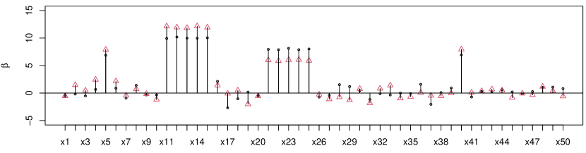
(a) LAD estimates ($\lambda_{1}=\lambda_{2}=0$).

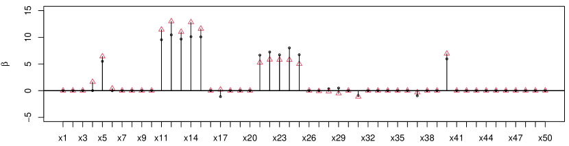
(b) LAD-lasso estimates ($\lambda_{1}=0.2,\lambda_{2}=0$).

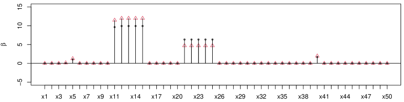
(c) Fused LAD-lasso estimates ($\lambda_{1}=0.2,\lambda_{2}=0.1$).

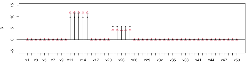
(d) Fused LAD-lasso estimates ($\lambda_{1}=0.2,\lambda_{2}=0.2$).

Figure 1: Simulation results illustrating the modelling techniques. The two outcome variables are marked with $\circ$ and ${\color[rgb]{1,0,0}\triangle}$.

5 Application in disability retirement analysis

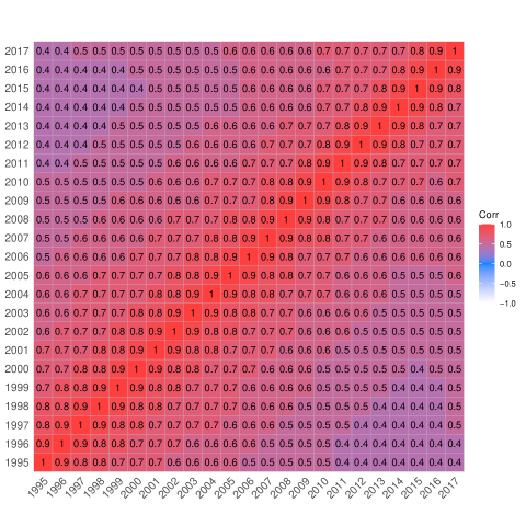
Figure 5: The correlation plot of the wages from years 1995 to 2017 (variables x1-x22).

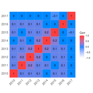
Figure 6: The correlation plot of the long-term sickness benefit days from years 2010 to 2017 (variables x23-x30).

In this section we use the presented fused methodology to analyze retirement behaviour. The data consist of disability pension retirees in Finnish statutory earnings-related pension system for the public sector employees (both genders together). A random sample of 4,069 ($n\gg p$) municipal employees is drawn from the comprehensive administrative registers. The study-design includes three outcomes: length of working life (years) by the end of 2016, amount of final pension (Eur/month in 2017 price level) in 2017, and age at retirement (years) in 2017. The explaining variables include: monthly pensionable wages in 1995-2017 (x1-x22) and long-term sickness benefit days in 2010-2017 (x23-x30), both measured yearly. The consecutive wage observations are highly correlated (see Figure 5), whereas among benefit days the correlation is relatively mild (see Figure 6). The design allows us to illustrate the block-structure in the covariates and robustness of the estimates in the multi-outcome situation.

The distributions of the outcomes have long tails, both left and right, and they also contain zeros (see Figure 2). The distributions of explaining variables have long right tails and excess number of zeros, which have a real-life relevance (see Figure 3). In the subsequent analysis wages and pensions are transformed using asinh transformation (e.g.,[1]). Long-term sickness is oftentimes associated with deteriorating work ability and may lead to permanent disability, but in many cases work ability is lost without prolonged illness, and therefore we observe excess number of zeros in the measure. A note is in order on the fact that in practice zero yearly wages during life-course follow from absence from work for different reasons, such as, working in private sector or as self-employed, or drawing other social security benefits (e.g., unemployment, parental leaves). From Figure 3 we can also see that the wage distribution contains some outlying observations which challenge the existing methods.

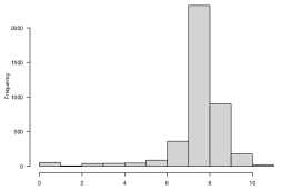
(a) Asinh of earnings-related pension

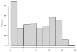
(b) Length of working-life

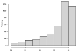
(c) Retirement age

Figure 2: Histograms of outcome variables: asinh earnings-related pension (a), length of working life (b) and retirement age (c).

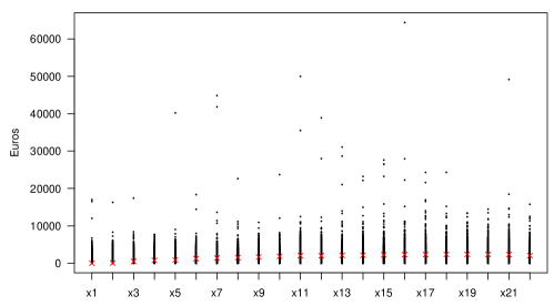
(a) Monthly wages

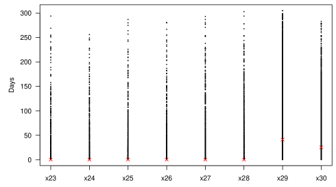
(b) Long-term sickness benefit days

Figure 3: Scatter plots of explaining variables: monthly wages (a) and long-term sickness benefit days (b). Median is marked with $\times$.

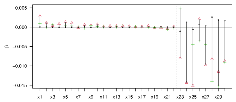
(a) LAD estimates ($\lambda_{1}=\lambda_{2}=0$).

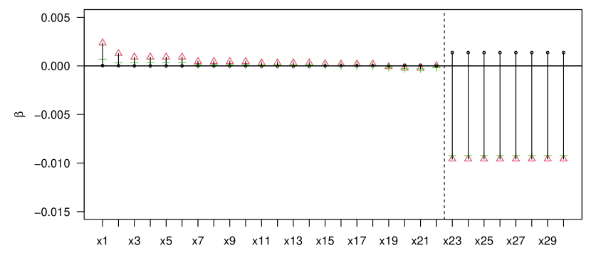
(b) Fused LAD-lasso estimates ($\lambda_{1}=0.03,\lambda_{2}=9.13$).

Figure 4: LAD-estimates and fused LAD-lasso estimates. Outcome markers: length of working life (${\color[rgb]{1,0,0}\triangle}$), retirement age (${\color[rgb]{0,1,0}+}$) and amount of pension ($\circ$). Explaining variables: asinh monthly wages in 1995-2017 (x1-x22) and long-term sickness days in 2010-2017 (x23-x30).

From Figures 4a we can see the coefficient estimates for ordinary LAD-lasso without the fusion penalty, and fused LAD-lasso for the three outcomes. In fused LAD-lasso the covariate blocks $\gamma_{j}$ are defined for wages (x1-x22) and benefit days (x23-x30).

The ordinary LAD regression estimates for wages indicate higher values for distant wages especially for outcomes: length of working life and retirement age. In benefit days we see high variation across outcomes and time-points.

Next, we switch to fused LAD-lasso estimation results. First step of the analysis is to evaluate the $\lambda_{1}$ and $\lambda_{2}$ parameters. Since there are currently no alternative criterion for the model selection, we used the 5-fold cross-validation criterion (CV criterion) similar to [16]. As a search procedure we use grid search, which is a common and easy to implement model selection method, where a subset of parameter values are fully searched. The contour plot of the parameter space and the minimum values of the $\lambda$’s are given in Figure 7 in appendix. From Figure 4 we can see the results of the fused LAD-lasso estimation with the CV criterion. The results indicate similar estimates for wages as in ordinary LAD-lasso. We can see that the fusion smooths the coefficient estimates of the outcomes, especially between distant time-points (x1-x17). The time-points for benefit days (x23-x30) are smoothed in total. We can see that length of working life and retirement age get negative estimates (-0.00957 and -0.00922), while the amount of pension gets positive estimates (0.00137).

When comparing ordinary and fused techniques, we can see that fused technique yields lower estimates in absolute terms, which is as expected.

Finally, we can observe that there is an issue with the spike in the wage estimate (x1) for the length of working life in both analyzes. In practice, the spike in the estimate for wages in x1 (year 1995) on pension is a result of high correlation between consecutive wages. This multicollinearity in regression analysis can, in general, lead to instability in the estimates, and to a problem where the explained variance is allocated arbitrarily among the correlated explanatory variables (see [5]). To some degree the proposed fused LAD-lasso technique alleviates these phenomena, but the issue needs to be considered by the practitioners.

6 Conclusion and discussion

We presented the multi-outcome fused LAD-lasso, which introduces the robust LAD-lasso regression with a fusion penalty into a multi-outcome context. In a simulation study, we pointed out the pros of the proposed method to both achieving variable selection and finding the true correlated groups in the sequential data. In a disability retirement study, we applied the method to a challenging real-life data set, with outlier observations and a skewed distribution of outcome variables. The proposed method provided insights to the analysis by smoothing the highly correlated neighboring covariates. We believe that practitioners in many fields of science familiar with regression techniques could find the fused LAD-lasso modelling approach useful when robust estimates are required.

A note is in order on the fact that in high-dimensional data the lasso-estimated non-zero coefficients may still contain some false positives. To filter out false positives, stability selection has been proposed as an additional confirmatory step after lasso-estimated variable selection [15]. This kind of confirmatory step is also known as post-selection inference; see a recent review on the topic [34]. This step was omitted here but it may be beneficial to include it in the analysis if the consistency of the variable selection is one of the main requirements.

In the disability retirement study, the evaluation of optimal tuning parameters $\lambda_{1}$ and $\lambda_{2}$ was accomplished with a CV criterion using grid search to sift through the possible values of $\lambda_{1}$ and $\lambda_{2}$. However, when the models are complex and the number of observations is high, applying more advanced methods such as Bayesian optimization would be beneficial in terms of computational time [21]. In essence, Bayesian optimization constructs a probabilistic model for the objective function, which is then iteratively updated based on the evaluations with different values of hyperparameters ($\lambda_{1}$ and $\lambda_{2}$ in our case), while taking into account the uncertainty of the model [23]. Although the overall computational time in our analysis was reasonable, the use of Bayesian optimization instead of CV may be necessary with larger data sets in the future.

The LAD-lasso modelling approach, in general, would benefit from further development. First, the model selection criterion (to select appropriate $\lambda_{1}$ and $\lambda_{2}$ values) naturally have influence on the results. Currently, the CV criterion is used, but in the future BIC-type criterion could broaden the options for model selection and validation. Second, in many empirical applications there is an issue with the excess number of zeros in explanatory variables. To alleviate the influence of zeros, an adaptive LAD-lasso has been proposed by [16] and later applied in [9]. The adaptive technique could be merged with the presented fused approach. Third, issues of post-selection inference and confidence intervals of the regression coefficients (cf. stability selection) in the LAD-lasso context needs more attention in the future.

Disclosure of interest

The authors report no conflict of interest.

ORCID

Jyrki Möttönen: https://orcid.org/0000-0002-6270-2556
Tero Lähderanta: https://orcid.org/0000-0001-5856-2899
Janne Salonen: https://orcid.org/0000-0002-0595-6226
Mikko J. Sillanpää: https://orcid.org/0000-0003-2808-2768

Appendix A Additional visualizations in the disability retirement analysis

Figure 7: Contour plot of cross-validation mean absolute errors. The global minimum point ($\lambda_{1}=0.03$, $\lambda_{2}=9.13$ ) is marked with $+$.

References

- [1] M.F. Bellemare and C.J. Wichman, Elasticities and the inverse hyperbolic sine transformation, Oxford Bulletin of Economics and Statistics 82 (2020), pp. 50–61. Available at https://onlinelibrary.wiley.com/doi/abs/10.1111/obes.12325.
- [2] L. Chen, M. Pourahmadi, and M. Maadooliat, Regularized multivariate regression models with skew-t error distributions, Journal of Statistical Planning and Inference 149 (2014), pp. 125–139. Available at https://doi.org/10.1016/j.jspi.2014.02.001.
- [3] S. Corsaro, V. De Simone, and Z. Marino, Fused lasso approach in portfolio selection, Annals of Operations Research 299 (2021), pp. 47–59. Available at https://doi.org/10.1007/s10479-019-03289-w.
- [4] P. Danaher, P. Wang, and D.M. Witten, The joint graphical lasso for inverse covariance estimation across multiple classes, J R Stat Soc Series B Stat Methodol. 76 (2014), pp. 373–397. Available at https://doi.org/10.1111/rssb.12033.
- [5] D.E. Farrar and R.R. Glauber, Multicollinearity in regression analysis: The problem revisited, The Review of Economics and Statistics 49 (1967), pp. 92–107. Available at https://doi.org/10.2307/1937887.
- [6] F. Heinzl and G. Tutz, Clustering in linear-mixed models with a group fused lasso penalty, Biometrical Journal 56 (2014), pp. 44–68. Available at https://doi.org/10.1002/bimj.201200111.
- [7] T. Hocking, J.P. Vert, F. Bach, and A. Joulin, Clusterpath An Algorithm for Clustering using Convex Fusion Penalties, in Proceedings of the 28 the International Conference on Machine Learning, Bellevue, WA, USA. 2011, pp. 745–752. Available at https://www.di.ens.fr/~fbach/419_icmlpaper.pdf.
- [8] Z.T. Ke, J. Fan, and Y. Wu, Homogeneity pursuit, Journal of the American Statistical Association 110 (2015), pp. 175–194. Available at http://dx.doi.org/10.1080/01621459.2014.892882.
- [9] T. Lähderanta, J. Salonen, J. Möttönen, and M.J. Sillanpää, Modelling old-age retirement: An adaptive multi-outcome LAD-lasso regression approach, International Social Security Review 75 (2022), pp. 3–29. Available at https://doi.org/10.1111/issr.12287.
- [10] S. Land and J. Friedman, Variable fusion: a new method of adaptive signal regression, Tech. Rep., Department of Statistics, Stanford University, Stanford, 1996. Available at https://www.stat.cmu.edu/tr/tr656/tr656.ps.
- [11] K.L. Lange, R.J.A. Little, and J.M.G. Taylor, Robust statistical modeling using the t distribution, Journal of the American Statistical Association 84 (1989), pp. 881–896. Available at https://doi.org/10.2307/2290063.
- [12] Z. Li, J. Möttönen, and M.J. Sillanpää, A robust multiple-locus method for quantitative trait locus analysis of non-normally distributed multiple traits, Heredity 115 (2015), pp. 556–564. Available at https://doi.org/10.1038/hdy.2015.61.
- [13] Z. Li and M.J. Sillanpää, Overview of LASSO-related penalized regression methods for quantitative trait mapping and genomic selection, Theoretical and Applied Genetics 125 (2012), pp. 419–435. Available at https://doi.org/10.1007/s00122-012-1892-9.
- [14] Y. Liu, J. Tao, H. Zhang, X.C. Xu, and L.C. Kong, Fused lasso penalized least absolute deviation estimator for high dimensional linear regression, Numerical Algebra, Control & Optimization 8 (2018), pp. 97–117. Available at https://dx.doi.org/10.3934/naco.2018006.
- [15] N. Meinshausen and P. Bühlmann, Stability selection, Journal of the Royal Statistical Society: Series B (Statistical Methodology) 72 (2010), pp. 417–473. Available at https://doi.org/10.1111/j.1467-9868.2010.00740.x.
- [16] J. Möttönen, T. Lähderanta, J. Salonen, and M.J. Sillanpää, Reducing bias and alleviating the influence of excess of zeros with multioutcome adaptive lad-lasso (2021). Available at https://arxiv.org/abs/2109.04798.
- [17] J. Möttönen and M.J. Sillanpää, Robust variable selection and coefficient estimation in multivariate multiple regression using LAD-lasso, in Modern Nonparametric, Robust and Multivariate Methods: Festschrift in Honour of Hannu Oja, K. Nordhausen and S. Taskinen, eds., Springer International Publishing, Cham, 2015, pp. 235–247. Available at https://doi.org/10.1007/978-3-319-22404-6_14.
- [18] K. Nordhausen, J. Möttönen, and H. Oja, MNM: Multivariate nonparametric methods - An approach based on spatial signs and ranks (2016). Available at http://CRAN.R-project.org/package=MNM, R package version 1.0-2.
- [19] K. Nordhausen and H. Oja, Multivariate methods: The package MNM, Journal of Statistical Software 43 (2011), pp. 1–28. Available at https://doi.org/10.18637/jss.v043.i05.
- [20] H. Oja, Multivariate Nonparametric Methods with R - An Approach Based on Spatial Signs and Ranks, Springer, New York, 2010, Available at http://dx.doi.org/10.1007/978-1-4419-0468-3.
- [21] B. Shahriari, K. Swersky, Z. Wang, R.P. Adams, and N. de Freitas, Taking the human out of the loop: A review of bayesian optimization, Proceedings of the IEEE 104 (2016), p. 148–175.
- [22] Y. She, Sparse regression with exact clustering, Electronic Journal of Statistics 4 (2010), pp. 1055 – 1096. Available at https://doi.org/10.1214/10-EJS578.
- [23] J. Snoek, H. Larochelle, and R.P. Adams, Practical Bayesian Optimization of Machine Learning Algorithms, in Advances in Neural Information Processing Systems, Vol. 25. Curran Associates, Inc., 2012. Available at https://proceedings.neurips.cc/paper/2012/hash/05311655a15b75fab86956663e1819cd-Abstract.html.
- [24] Y. Sun, H.J. Wang, and M. Fuentes, Fused adaptive lasso for spatial and temporal quantile function estimation, Technometrics 8 (2018), pp. 127–137. Available at http://dx.doi.org/10.1080/00401706.2015.1017115.
- [25] R. Tibshirani, Regression shrinkage and selection via the lasso, Journal of the Royal Statistical Society. Series B 58 (1996), pp. 267–288. Available at https://www.jstor.org/stable/2346178.
- [26] R. Tibshirani, M. Saunders, S. Rosset, J. Zhu, and K. Knight, Sparsity and smoothness via the fused lasso, Journal of the Royal Statistical Society: Series B (Statistical Methodology) 67 (2005), pp. 91–108. Available at https://doi.org/10.1111/j.1467-9868.2005.00490.x.
- [27] R. Tibshirani and P. Wang, Spatial smoothing and hot spot detection for cgh data using the fused lasso, Biostatistics 9 (2008), pp. 18–29. Available at https://doi.org/10.1093/biostatistics/kxm013.
- [28] R.J. Tibshirani and J. Taylor, The solution path of the generalized lasso, The Annals of Statistics 39 (2011), pp. 1335–1371. Available at https://www.jstor.org/stable/23033600.
- [29] B.A. Turlach, W.N. Venables, and S.J. Wright, Simultaneous variable selection, Technometrics 47 (2005), pp. 349–363. Available at https://doi.org/10.1198/004017005000000139.
- [30] H. Wang and C. Leng, A note on adaptive group lasso, Computational Statistics & Data Analysis 52 (2008), pp. 5277–5286. Available at https://doi.org/10.1016/j.csda.2008.05.006.
- [31] R. Yang, X. Wang, J. Li, and H. Deng, Bayesian robust analysis for genetic architecture of quantitative traits, Bioinformatics 25 (2009), pp. 1033–1039. Available at https://doi.org/10.1093/bioinformatics/btn558.
- [32] M. Yuan, A. Ekici, Z. Lu, and R. Monteiro, Dimension reduction and coefficient estimation in multivariate linear regression, Journal of the Royal Statistical Society. Series B 69 (2007), pp. 329–346. Available at https://www.jstor.org/stable/4623272.
- [33] M. Yuan and Y. Lin, Model selection and estimation in regression with grouped variables, Journal of the Royal Statistical Society. Series B 68 (2006), pp. 49–67. Available at https://doi.org/10.1111/j.1467-9868.2005.00532.x.
- [34] D. Zhang, A. Khalili, and M. Asgharian, Post-model-selection inference in linear regression models: An integrated review, Statistics Surveys 16 (2022), pp. 86–136. Available at https://doi.org/10.1214/22-SS135.
- [35] H. Zou and T. Hastie, Regularization and variable selection via the elastic net, Journal of the Royal Statistical Society: Series B (Statistical Methodology) 67 (2005), pp. 301–320. Available at https://doi.org/10.1111/j.1467-9868.2005.00503.x.